Spatio-Temporal Super-Resolution Data Assimilation (SRDA) Utilizing Deep Neural Networks with Domain Generalization
Abstract
Deep learning has recently gained attention in the atmospheric and oceanic sciences for its potential to improve the accuracy of numerical simulations or to reduce computational costs. Super-resolution is one such technique for high-resolution inference from low-resolution data. This paper proposes a new scheme, called four-dimensional super-resolution data assimilation (4D-SRDA). This framework calculates the time evolution of a system from low-resolution simulations using a physics-based model, while a trained neural network simultaneously performs data assimilation and spatio-temporal super-resolution. The use of low-resolution simulations without ensemble members reduces the computational cost of obtaining inferences at high spatio-temporal resolution. In 4D-SRDA, physics-based simulations and neural-network inferences are performed alternately, possibly causing a domain shift, i.e., a statistical difference between the training and test data, especially in offline training. Domain shifts can reduce the accuracy of inference. To mitigate this risk, we developed super-resolution mixup (SR-mixup)–a data augmentation method for domain generalization. SR-mixup creates a linear combination of randomly sampled inputs, resulting in synthetic data with a different distribution from the original data. The proposed methods were validated using an idealized barotropic ocean jet with supervised learning. The results suggest that the combination of 4D-SRDA and SR-mixup is effective for robust inference cycles. This study highlights the potential of super-resolution and domain-generalization techniques, in the field of data assimilation, especially for the integration of physics-based and data-driven models.
Journal of Advances in Modeling Earth Systems (JAMES)
Global Scientific Information and Computing Center, Tokyo Institute of Technology, 2-12-1 Ookayama, Meguro-ku, Tokyo 1528550, Japan
Yuki Yasudayasuda.y.aa@m.titech.ac.jp
We propose a neural network-based scheme for data assimilation and spatio-temporal super-resolution using physics-based simulations
A data-augmentation technique was developed to improve the robustness of inference in the fusion of data-driven and physics-based models
A test with idealized ocean jets showed that the proposed approach efficiently infers high-resolution results with ensuring the robustness
Plain Language Summary
One challenge in the Earth sciences is the simulation of atmospheric and oceanic processes with high accuracy or at high spatio-temporal resolution. The neural network, a model developed in the field of artificial intelligence, has recently gained attention for its potential to learn the relationship between any variables from a sufficient amount of data. For example, a neural network can be trained to make high-resolution images from low-resolution images. This process is called super-resolution. We propose the incorporation of a neural network for super-resolution into an atmospheric or ocean model that performs numerical simulations at low resolution. Since the atmospheric or ocean model is of low resolution, the proposed framework is computationally efficient while still allowing for high-resolution results with the aid of the neural network. Furthermore, to make the inference accurate, observation data are fused with atmospheric or ocean predictions in the neural network. In real-world applications, it is important to make predictions robust to noise from various factors. Accordingly, we developed a new technique where certain noise is added during the training of the neural network. The approach proposed here can efficiently compute high-resolution predictions of the atmosphere and ocean without compromising robustness.
1 Introduction
Numerical simulation is an essential tool in the atmospheric and oceanic sciences. Despite the ever-increasing computer resources, it may still be difficult to conduct numerical simulations at high resolution or with high accuracy. One solution is to employ data-driven models such as neural networks (NNs) [Brunton \BOthers. (\APACyear2020), Duraisamy (\APACyear2021), Kashinath \BOthers. (\APACyear2021)]. For instance, NNs have been used for surrogate modeling of the Navier-Stokes equations, subgrid-scale modeling of Reynolds stress tensors, and super-resolution of fluid flows. These NNs can make numerical simulations more efficient or more accurate.
Super-resolution (SR) refers to techniques that infer high-resolution (HR) images from low-resolution (LR) images. Methods based on deep learning have been studied in computer vision [<]e.g.,¿Dong+2014ECCV, Ha+2019, Anwar+2020ACMCS. The success of such NNs has promoted the applications of SR to atmospheric and oceanic data [<]e.g.,¿[]Ducournau+2016PRRS, Vandal+2017ACM, Onishi+2019SOLA, Stengel+2020PNAS, Wang+2021GMD, Wu+2021GRL, Yasuda+2023BAE. One example is SR simulation [Onishi \BOthers. (\APACyear2019), J. Wang \BOthers. (\APACyear2021), Wu \BOthers. (\APACyear2021)]. With this scheme, time evolution is calculated from LR simulations using a physics-based model, and HR inferences are obtained by inputting the LR results into a trained NN. Super-resolution simulation is computationally efficient because it requires only LR simulations using a physics-based model, and the elapsed time of inference by a NN is usually negligible. However, there is a concern that LR simulations may deviate from the true state because of unresolved processes. Data assimilation may be useful for reducing such deviation.
Data assimilation (DA) is a framework that estimates the state of a system based on observations and background states provided by a model [Asch \BOthers. (\APACyear2016)]. Methods of DA are typically variational or statistical, with NNs being applied to both types. Recent progress in the application of NNs to DA has been summarized in a review [Cheng \BOthers. (\APACyear2023)]. Variational methods, such as 4D-Var, are analogous to deep learning, in that both employ adjoint backpropagation [Abarbanel \BOthers. (\APACyear2018), Chen \BOthers. (\APACyear2018)]. The minimization of variational cost can be conducted with NNs, achieving more precise 4D-Var estimations [Fablet \BOthers. (\APACyear2021), Beauchamp \BOthers. (\APACyear2022)]. Neural networks have also been incorporated into statistical methods, such as ensemble Kalman filters (EnKFs). To reduce the computational cost of calculating ensemble evolution, the system model can be replaced with a NN [Ouala \BOthers. (\APACyear2018), Chattopadhyay \BOthers. (\APACyear2022)]. In addition, the analysis step can be conducted in low-dimensional latent spaces to further increase computational efficiency [Amendola \BOthers. (\APACyear2021), Peyron \BOthers. (\APACyear2021), C. Liu \BOthers. (\APACyear2022)]. Instead of replacing system models, ensemble members can be obtained using generative models, such as variational autoencoders (VAEs), which also reduce computation time [Grooms (\APACyear2021), Yang \BBA Grooms (\APACyear2021)].
Super-resolution has recently been included in DA processes [Barthélémy \BOthers. (\APACyear2022)], as super-resolution data assimilation (SRDA), which applies a statistical DA method, such as EnKF, to flow fields super-resolved by a NN. SRDA can be interpreted as a fusion of SR simulation and DA. Specifically, the time evolution of an ensemble is obtained from LR simulations via a physics-based model, as in SR simulation. The NN independently super-resolves each LR result in the ensemble. Observations are then assimilated into these super-resolved HR data. The obtained HR analysis is mapped to the LR space using algebraic methods, such as linear interpolation, and this mapped state provides the initial condition for the next assimilation cycle. SRDA performs super-resolution and data assimilation separately, making it easy to incorporate into an existing DA framework. Some studies have shown that NNs can perform the entire or a part of the analysis step. For instance, NNs can directly infer the analysis states [Krishnan \BOthers. (\APACyear2015), Fraccaro \BOthers. (\APACyear2017)] or can estimate background error covariance matrices [Ouala \BOthers. (\APACyear2018), Grooms (\APACyear2021)]. These studies imply the potential for simultaneous SR and DA. However, to the authors’ knowledge, SR has yet to be fully studied in the context of DA and such a proof of concept has not been demonstrated.
In SRDA [Barthélémy \BOthers. (\APACyear2022)], physics-based simulations and NN inferences are alternated, potentially causing a domain shift [<]e.g.,¿MorenoTorres+2012PR, in which the statistical distribution differs between the training and test data. Domain shifts can occur whenever physics-based simulations and NN inferences are interdependent. For instance, if training data are generated in advance via physics-based simulations (i.e., offline training), a domain shift will occur because the training data are independent of the NN inference. Although this issue is briefly mentioned by \citeABarthelemy+2022OD, it has not been investigated. Online training provides a potential solution to this domain shift [Rasp (\APACyear2020)]. In this approach, training data are updated during the optimization of NNs through physics-based simulations [<]e.g.,¿Krasnopolsky+2020arXiv. However, online training may be computationally intensive and is not always feasible.
Domain generalization aims to improve generalizability across datasets with different distributions and to overcome domain shift problems [<]e.g.,¿Wang+2022IEEE, Zhou+2022IEEE. Domain generalization is similar to transfer learning, but differs in access to the test-data distribution. In transfer learning, a pre-trained NN is fine-tuned using small samples with the same distribution as the test data. In contrast, in scenarios of domain generalization, fine-tuning is impossible because such samples are not available. In other words, the test-data distribution remains unknown up to the test phase. Domain-generalization methods may be useful for fusing data-driven and physics-based models; however, the applicability of domain generalization in applying NNs to fluid systems remains unclear, particularly for atmospheric or oceanic data assimilation.
In this study, we propose a novel data-assimilation scheme, four-dimensional SRDA (4D-SRDA), incorporating SR-mixup—a novel domain-generalization technique. In 4D-SRDA, DA and spatio-temporal SR are performed simultaneously by a NN, while the system’s time evolution is obtained from physics-based LR simulations. This scheme does not require ensemble members and is computationally efficient. To mitigate the risk of domain shifts and the associated deterioration in inference accuracy, we employed SR-mixup—a data-augmentation technique based on the mixup method [Zhang \BOthers. (\APACyear2018), Yao \BOthers. (\APACyear2022)]. The validity of this scheme was demonstrated using an idealized barotropic ocean jet [David \BOthers. (\APACyear2017)]. The 4D-SRDA and SR-mixup are applicable to physics-based models that use gridded input and output data. This study implies the potential of SR and domain generalization, in the field of DA, for integrating physics-based and data-driven models.
The remainder of the paper is organized as follows: 4D-SRDA is first proposed in Section 2. SR-mixup is then independently presented in Section 3. Numerical experiments are described in Section 4, where the NN in the 4D-SRDA system is trained using SR-mixup. Section 5 evaluates the performance of the 4D-SRDA system and discusses the robustness of inference enhanced by SR-mixup. Section 6 presents the conclusions.
2 Four-Dimensional Super-Resolution Data Assimilation (4D-SRDA)
2.1 General Concept
4D-SRDA comprises a NN and a physics-based model. The latter is typically an atmosphere or ocean model and is simply referred to as a “fluid model.” The system’s time evolution is calculated from LR simulations using the fluid model. The DA and spatio-temporal SR are performed simultaneously using the NN. Unlike EnKF and 4D-Var, the proposed method does not require ensemble members or iterative calculations and is computationally efficient.
The calculation process in each assimilation cycle is shown in Figure 1. Consider the time series of observations and fluid-model states. The former are time-stamped and geolocated point-cloud data, while the latter are LR grid-point data. The LR fluid-model states generally include past, present, and future times, whereas observations are available only for the past and present. Using these two input types, the NN infers a flow-field time series at high spatio-temporal resolution. In the NN, the observations are converted from point-cloud to grid-point data. The converted observations and the LR model states are fused through a low-dimensional latent space by utilizing an encoder–decoder architecture. Because of the encoder, the observations do not necessarily have to be physical quantities—they can also be arbitrary quantities correlated with the true state of the system. In principle, the nonlinear mapper in Figure 1 represents any mapping in the latent space, including temporal SR (Section 4.2), while its specific form is determined by training. A snapshot of the inferred HR states is downsampled to the LR grid space using an algebraic operation, such as linear interpolation. The obtained LR snapshot is regarded as the analysis (the initial condition), from which an LR fluid simulation is conducted. The obtained output—a time series of LR model states—is used as input to the NN in the next assimilation cycle. This process (Figure 1) is repeated once new observations are obtained.
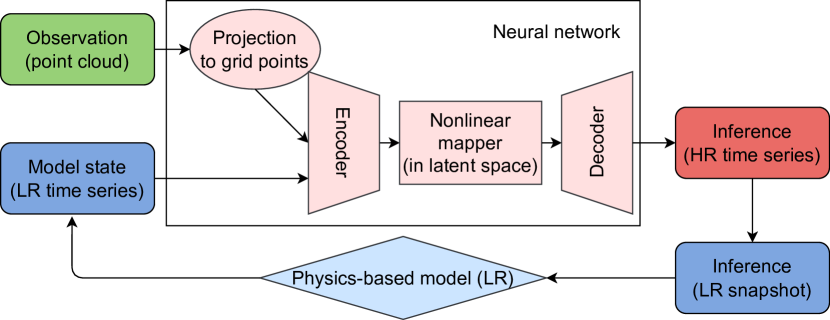
There are two key differences between 4D-SRDA and SRDA [Barthélémy \BOthers. (\APACyear2022)]. First, in 4D-SRDA, the input to the NN contains a time series of fluid-model states, whereas in SRDA, the input is a snapshot of these states. Second, in 4D-SRDA, the NN simultaneously performs DA and spatio-temporal SR, whereas in SRDA, the NN conducts spatial SR followed by a statistical DA (e.g., EnKF). Both 4D-SRDA and SRDA obtain the time evolution of the system via LR fluid simulation. SRDA is easily applicable to existing DA frameworks because it performs SR and DA separately; however, this separation may not fully optimize SR inference for DA. In contrast, 4D-SRDA may achieve more accurate inference because it adopts end-to-end learning that simultaneously optimizes the SR and DA processes; however, the feasibility of such learning is unclear. This study presents an offline supervised learning method employing a new technique, SR-mixup, which mitigates the influence of domain shift (Section 3). Unsupervised or online learning is another important topic for future research.
2.2 Algorithm of 4D-SRDA Inference
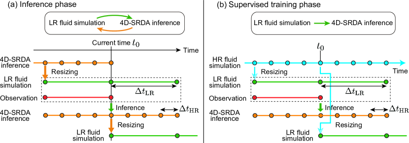
The details of the 4D-SRDA inference are given for one assimilation cycle shown in Figure 2a, where the assimilation window has the same length as the forecast period. This configuration is used for the numerical experiments in Sections 4 and 5. More general cases are briefly discussed later in this section.
We first describe the input to the NN. A time series of LR states is obtained by numerically integrating the LR fluid model:
| (1) |
where the current time is denoted by and is the LR time step for the output. The initial condition is given by the previous analysis state; and are the current and future states estimated by the LR fluid model, respectively. Each snapshot is defined on the LR spatial grid points and is generally composed of various three-dimensional field quantities, such as velocity and temperature. Observations are assumed to be given as:
| (2) |
which does not include the future time . The observation also consists of several three-dimensional quantities and is defined on the HR spatial grid points, including missing data. The HR spatial resolution is assumed to be four times finer than the LR resolution.
A trained NN, denoted by , super-resolves the time series of the LR fluid-model states while incorporating the observations:
| (3) |
The time series of is composed of the same three-dimensional quantities as , whereas is obtained on the HR spatio-temporal grid points. For instance, in Figure 2a, the HR temporal resolution is four times finer, i.e., . A hat indicates that is a NN inference. The input of the future LR state is expected to serve as auxiliary information for time evolution, helping the NN infer the HR states at future times. The output for the current time is mapped onto the LR spatial grid points using an algebraic method, such as linear interpolation. This mapped state is utilized as the initial condition for the LR fluid model in the next assimilation cycle, in which the current time is moved to (the assimilation interval is ). The outputs at the other time steps, such as and , are not used in the next assimilation cycle.
Various modifications of the above algorithm are possible. For instance, more LR time steps can be included in the inference, whereas three time steps are used in Equation 3; the length of the assimilation window or forecast period can be varied, whereas both have the same length in Figure 2a; the scale factor of the spatial or temporal SR can be changed, whereas both factors are set to four above; and the past data can be eliminated from the input to the NN, leaving only the present and future input data, in contrast to Equation 3.
In this research, two assumptions are made for observation data: (i) mappability to any space-time point and (ii) statistical stationarity. Equation 2 is based on the first assumption; that is, the observations can be mapped to the HR spatial grid points and LR time points by spatio-temporal interpolation. In real-world applications, such interpolation cannot be directly applied to integrated quantities. For instance, mapping cumulative precipitation to the time axis is not straightforward. Investigating the treatment of integrated quantities is beyond the scope of this study. Thus, we make the first assumption. NNs can be effective in solving such an inverse problem. In particular, the reconstruction techniques of three-dimensional point cloud data from two-dimensional images [<]e.g.,¿Mandikal+2018BMVC, Li+2020IEEE would be useful to assimilate integrated observations.
The second assumption covers stationarity in terms of both temporal and spatial statistics, which indicates that observation errors, including measurement and representativeness errors, are stationary. This assumption facilitates the representation learning of observations with missing data (Section 5.2), but is not necessarily satisfied in real-world applications. It is worth noting here that the statistical stationarity does not imply temporal steadiness. Indeed, in Sections 4 and 5, the spatial density of observations is constant, while the observed grid points vary in time. This change in observed locations is accounted for by the translation equivariance of the convolution operation [<]e.g.,¿Cohen+2019NIPS; i.e., features can be extracted by convolution independently of observed locations. This implies that the local equivariance improves the generalizability for changes in observation data. For instance, there may be cases where the stationarity is broken globally but preserved locally, such as in the expansion of observation networks. Various equivariant NNs have recently been studied [<]e.g.,¿Cohen+2019NIPS, Sosnovik2021, including graph NNs [Fuchs \BOthers. (\APACyear2020)]. Such an advanced architecture will need to be incorporated into 4D-SRDA for practical applications where observations are not stationary.
2.3 A Case of Supervised Learning
In this study, the NN involved in 4D-SRDA is trained using an offline supervised learning method. Offline means that training data are generated in advance from LR fluid simulations in which the NN inference is not considered; in other words, the feedback from the NN to the LR fluid model is not considered in the offline training. Supervised learning requires HR target data that can be interpreted as the true state of the atmosphere or ocean. In practice, such data can be obtained from HR reanalysis datasets. Thus, in the case of supervised learning, 4D-SRDA is a computationally efficient alternative for generating the HR reanalysis.
Figure 2b describes the supervised learning that corresponds to the inference in Figure 2a. Consider the target variables, namely the HR time series , where each snapshot is defined on the HR spatial grid points. Training datasets are created at a constant interval of , which is equal to the assimilation interval in the inference phase (Figure 2a). Here, we explain the generation of a sample of the dataset for reference time . The initial condition for the LR fluid model is given by resizing the HR snapshot by an algebraic method, such as linear interpolation. This initial condition is interpreted as the analysis state from the previous assimilation cycle. The LR fluid model is then numerically integrated from to to obtain a time series of the LR states , as in Equation 1. For observations, since the target variables are obtained from the HR reanalysis dataset, the same observations used to produce this reanalysis can be utilized in the training. By using spatio-temporal interpolation, the observations are generated at and , as in Equation 2. Consequently, the pair of the input and output is given by
| (4) |
Training data generation is repeated by varying at a constant interval of . When optimizing the NN, the inference is computed as in Equation 3, and the NN weights are updated based on the gradients of a given loss function.
The generation of the initial condition for the LR fluid model is different between the inference and training phases (Figure 2). Specifically, in the inference phase, the initial condition is obtained from the previous NN inference, while in the training phase, it is obtained from the HR target data. This difference results in a domain shift [<]e.g.,¿MorenoTorres+2012PR, namely a statistical difference in the input time series of LR states , which can be detrimental to 4D-SRDA performance. Indeed, a domain shift is inevitable in offline training because the training data are generated in advance independently of the NN inference. As a potential solution, we present a novel technique, SR-mixup.
3 Super-Resolution Mixup (SR-mixup)
SR-mixup is a data augmentation method for domain generalization. The algorithm can be applied to ordinary SR problems; thus, the following discussion is independent of 4D-SRDA. Before explaining SR-mixup, we will review the mixup method [Zhang \BOthers. (\APACyear2018), Yao \BOthers. (\APACyear2022)].
Mixup is a data augmentation method for supervised classification problems [Zhang \BOthers. (\APACyear2018)]. Consider a training dataset (), where is a numerical array, such as an image, and is the corresponding class label based on one-hot encoding. A linear combination is considered for two randomly sampled pairs, and :
| (5) | |||||
| (6) |
where the interpolation ratio is drawn from a beta distribution (). Supervised learning is performed for the mixed sample . Mixup is applied only during training, and not during the test phase. The random linear combination generates synthetic samples with a different distribution from the original training data. This mixing is expected to enhance robustness to domain shifts.
Several variants of mixup have been proposed [<]e.g.,¿Verma+2019PMLR, Mancini+2020ECCV, Yao+2022NIPS, most of which are intended for classification. \citeAYao+2022NIPS proposed a mixup for regression, C-Mixup, to address the issue that the linearity imposed via mixup reduces the accuracy of regression models when data are highly nonlinear. In C-Mixup, the linear combination in Equations 5 and 6 is created for similar randomly sampled pairs, where the similarity is measured using a distance metric between the labels and .
SR-mixup is based on C-Mixup. Super-resolution problems are treated as regression when SR models are trained via supervised learning [<]e.g.,¿Dong+2014ECCV. In such cases, the input is an LR image and the output is the corresponding HR image. The linear combination of similar HR images results in blurred images. Because the purpose of SR is to improve the resolution and clarity of LR images, C-Mixup may not be suitable for training SR models. We propose applying C-Mixup only to the input LR image. This method is called SR-mixup to emphasize the mixup for SR. Similarity is determined from the input instead of . SR-mixup is applicable to both supervised and unsupervised learning because the pairing between and is not required.
The SR-mixup algorithm consists of four steps and is employed only during training. Here, we explain the algorithm in a supervised setting, which is similar for unsupervised applications. First, a pair is drawn from the training dataset. Second, other pairs are randomly sampled, and pair is further extracted such that the Euclidean distance between and is the minimum. We adopted Euclidean distance as the dissimilarity measure, although other metrics can be used. Third, an interpolation ratio is drawn from the beta distribution . Fourth, a linear combination of inputs is created, , resulting in the augmented pair . The above four steps are repeated to generate a batch of data for optimizing the NN. The pairing of and is not essential, because the augmented input is produced independently from the labels and . The parameters were set to for the random sampling in the second step and for the beta distribution in the third step. Note that these parameters are context specific. In the present setting, and are regarded as statistically symmetric based on the symmetry of the beta distribution . This symmetry is discussed in Section 4.3.
4 Methods
Numerical experiments were performed to confirm the effectiveness of 4D-SRDA and SR-mixup. Specifically, we simulated idealized barotropic ocean jets and then conducted supervised learning. Hereafter, 4D-SRDA is referred to as ST-SRDA (spatio-temporal SRDA) because the barotropic jet was modeled as a two-dimensional flow and the sum of the spatial and temporal dimensions is not four.
4.1 Fluid Simulation
An idealized barotropic ocean jet was simulated in a two-dimensional periodic channel [David \BOthers. (\APACyear2017)]. The equatorial beta plane was utilized, where and are the zonal and meridional coordinates, respectively. The governing equations are as follows:
| (7) | |||||
| (8) | |||||
| (9) |
Equation 7 describes the evolution of vorticity with respect to time , where the left-hand side represents the advection of and the beta effect, and the right-hand side consists of linear drag, hyperviscosity, and forcing due to zonal wind stress . Equations 8 and 9 give the stream function and velocity , respectively. Wind stress is given by
| (10) |
where is determined such that the integral of is zero. The parameters in the governing equations were set as follows: , , , , , and . According to \citeADavid+2017OM, this configuration is within the parameter regime of mixing barriers with strong eddies, where coherent vortices remain in a statistically steady state (Section 5.1). The presence of these vortices simplifies the evaluation because the phase of vorticity, namely the large-scale flow structure, is related to errors in inference.
The initial condition was a superposition of a zonal jet and random perturbations. The zonal jet is given by
| (11) |
where . This initial jet satisfies the Rayleigh-Kuo inflection-point criterion, i.e., being somewhere in the domain, which is a necessary condition for barotropic instability. The perturbations were added to the vorticity field for each wavenumber, where the phase and amplitude were sampled from Gaussian distributions with means of and standard deviations of for the phase and for the amplitude. The simulation data for deep learning were generated by varying the random perturbations.
Numerical integration was performed using the modified Euler and pseudo-spectral methods. Three different resolutions were adopted: LR, HR, and ultra-HR (UHR). All configurations are summarized in Table 1. The integration time was from to for all experiments.
| Name | Grid size () | Cutoff wavenumber | Integration time step | Output time step |
|---|---|---|---|---|
| LR (low resolution) | 32 16 | 10 | 1.00 () | |
| HR (high resolution) | 128 64 | 42 | 0.25 () | |
| UHR (ultra-high resolution) | 1024 512 | 341 | 0.25 () |
4.2 Neural Network in the ST-SRDA System
The calculation process in the NN is simplified for potential application to three-dimensional flows. In particular, the temporal SR is separated from the spatial SR; that is, the temporal SR is performed in the nonlinear mapper, while the spatial SR is conducted in the decoder. In addition, the encoder and decoder act independently on the state at each time.
Figure 3 outlines the network architecture, which is based on U-Net [Ronneberger \BOthers. (\APACyear2015)]. U-Net architectures have been employed in the SR for fluid systems [<]e.g.,¿Jiang+2020ICHPC, Wang+2021PF, Hammoud+2022JAMES. The input and output of the NN are vorticity fields. Compared with Figure 1, this NN does not include a transformation from point-cloud to grid-point data because the observations are defined on the HR spatial grid points (Equations 2 and 3). Hyperparameters, such as the number of hidden layers, were tuned via a grid search. These parameters are presented in A. Details on the implementation of the NN are available at the Zenodo repository (see Open Research).
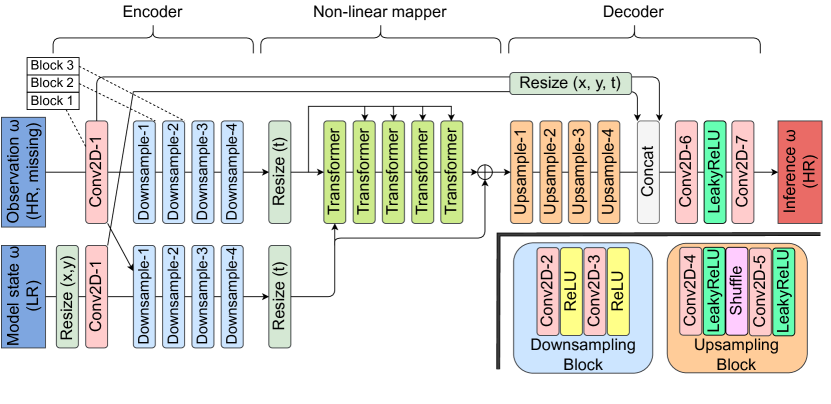
The encoder consists of four downsampling blocks. Each block begins with a convolution operation with a stride and halves the spatial size of the input array in the and dimensions. The LR model states are spatially resized using nearest neighbor interpolation to match the HR (“Resize (x,y)” in Figure 3) and then encoded while being combined with the observations. Additionally, the observations are independently encoded.
The nonlinear mapper contains five transformer-encoding blocks [Vaswani \BOthers. (\APACyear2017)]. The time interval of the input features is refined via linear interpolation to match the HR time steps (“Resize (t)” in Figure 3). This interpolation, followed by the nonlinear mapping, performs the temporal SR. The output from each transformer block is passed to the next, and the encoded observations are input to all blocks. Each block first computes weights for the input features across every time step pair and then outputs the weighted sums of the features. This processing, known as the scaled dot-product attention, incorporates temporal correlations into the nonlinear mapping [Vaswani \BOthers. (\APACyear2017), Niu \BOthers. (\APACyear2021)]. Finally, the encoded LR model states are added to the output via a skip connection.
The decoder comprises four upsampling blocks. Each block utilizes pixel shuffle [Shi \BOthers. (\APACyear2016)] to double the spatial size of the input array in the and dimensions. Using these four blocks, the spatial size of the output is restored to the HR grid size. The obtained output is concatenated with the features extracted by the first convolution in the NN, which are resized using linear interpolation along the space and time axes (“Resize (x,y,t)” in Figure 3). The final inference is given through the last three convolution and nonlinear layers.
In preprocessing, the vorticity at each grid point is transformed by the following formula:
| (12) |
The clipping function, defined as (), limits the value range to . This function acts independently on each element of the input array. Parameters and were determined such that 99.999% of the vorticity values were within the range of . As a result of this preprocessing, was considered a missing value and was substituted onto the HR grid points without observations.
4.3 Training and Testing Methods for the Neural Network
The training and testing methods for the NN are based on Sections 2.3 and 2.2, respectively. The relationship for the data along the time axis is the same as in Figure 2, where and . The assimilation interval is , which is approximately half of the advection time scale .
The training was performed using the HR simulation data, whereas in the test phase, ST-SRDA performance was evaluated with the UHR simulation results. The ST-SRDA is a surrogate scheme for generating HR reanalysis in the case of supervised learning (Section 2.3). In the training phase, the HR simulation data are considered to be derived from a reanalysis, while in the test phase, the UHR data are interpreted as the true state of the barotropic ocean jet system. The spatio-temporal resolution of the ST-SRDA output is always HR (Table 1); in the test, performance was measured by mapping the HR inference to UHR via bicubic interpolation. For comparison, EnKFs were applied to the LR and HR fluid models. The latter, EnKF at the HR, is interpreted as a model that generates the HR training data and is expected to provide a lower error bound for the ST-SRDA (The EnKFs are described in Section 4.4).
The scale factor for the SR is in both the spatial and temporal dimensions (i.e., , , and ). The target variable is a part of the HR vorticity time series, comprising nine data points with a time step of () (Figure 2b). The first four points are interpreted as the past, the middle point the present, and the last four points the future. The corresponding inputs to the NN are the time series of the observations and LR fluid-model states. The observations consist of two points in time, whereas the LR states consist of three points (Figure 2b). The time interval of both input time series is (). This configuration means that the NN performs the temporal SR with a factor of . Since the LR spatial grids () are four times coarser than the HR grids (), the spatial SR also has a factor of . The scale factor of is sufficiently high for real applications [Onishi \BOthers. (\APACyear2019), J. Wang \BOthers. (\APACyear2021)].
Synthetic observations were generated from the HR and UHR simulations in the training and test phases, respectively. For HR, observed grid points were randomly subsampled with a constant spatial spacing. Specifically, the spatial density of observations was constant, while observed grid points varied in time. For instance, when the vorticity is observed at every grids, the spatial density is approximately 1.56%. This ratio is referred to as the observation point ratio, which is defined as
| (13) |
The sensitivity to this ratio was assessed across experiments by varying it from 0.5% to 6.5%. At the unobserved grid points, Not a Numbers (NaNs) were substituted and replaced in subsequent preprocessing with missing values, i.e., zeros (Section 4.2). Spatially independent Gaussian noise was added to the subsampled vorticity, with a mean of and a standard deviation of , which is approximately 5% of the spatio-temporal average of the absolute values of vorticity. For UHR, the average pooling of an kernel was applied to the vorticity field to match the spatial size to that of the HR, and the above processing was applied.
The training and validation data were generated from the HR fluid simulations (Figure 2b). All simulations were terminated at , when the barotropic jet becomes a statistically steady state consisting of westward-propagating large-scale eddies [David \BOthers. (\APACyear2017)]. To increase dataset size, the initial random perturbations were varied randomly (Section 4.1), and 3,500 and 1,000 simulations were run for the training and validation dataset, respectively. Each HR simulation contained 23 LR-simulation cycles because of (i.e., ). In each cycle, the initial condition for the LR fluid model was given by applying a low-pass filter to the HR vorticity in the wavenumber domain. The total size of the training and validation dataset was 80,500 () and 23,000 (), respectively.
The NN was trained by employing SR-mixup and Adam optimization [Kingma \BBA Ba (\APACyear2015)]. For the loss function, we used the mean absolute error (MAE) of vorticity. The weights of the NN that resulted in the smallest validation MAE were stored after 1,000 epochs with a mini-batch size of 32. SR-mixup was applied only to the LR model states. SR-mixup is not necessary for the observation data, because they are independent of the NN inference and not subject to domain shifts. If SR-mixup were applied to data with missing values, such as observations, the linear interpolation would need to be replaced with a nearest neighbor interpolation using a threshold against .
In each iteration, SR-mixup generates a synthetic time series as in Equation 5:
where and denote the data indices, and is independent of and sampled from the beta distribution . Equation 4.3 is interpreted as the original time series being perturbed by a time series that is similar to in terms of Euclidean distance (Section 3). In training, was used as input instead of . The beta distribution was set to be symmetric (i.e., ) to increase the perturbation amplitude. The grid-wise relative error between two similar LR time series was found to be quite small ( 10%) due to the sufficiently large dataset size. As the dataset size decreases, the difference between and tends to increase, suggesting that needs to be biased toward , i.e., an asymmetric beta distribution is required to suppress the perturbation amplitude. Note that SR-mixup partially breaks the dynamical consistency in the LR time series; for instance, nonlinear conserved quantities, such as energy, are not constant in time. On the other hand, the linearity of SR-mixup indicates that linear constraints, such as Equations 8 and 9, are preserved because all physical quantities are linearly superposed by using the same weight of . Mixup, including SR-mixup, is a simple method for domain generalization [Zhang \BOthers. (\APACyear2018), Yao \BOthers. (\APACyear2022)]. Advanced methods, such as generative adversarial networks (GANs) [<]e.g.,¿Wang+2022IEEE, Zhou+2022IEEE may improve dynamical consistency.
The test method is the same as the inference method in Figure 2a, which repeats the feedback cycle between the NN and fluid model. In the first cycle, the initial condition for the LR fluid model was given by a superposition of random perturbations and the zonal jet (Equation 11) because of no NN inference, while in later cycles, the initial condition was obtained by applying the low-pass filter to the NN inference. Since the initial perturbations in the first cycle were random, the vorticity evolution would be largely different even using the HR fluid model. Here, 50 UHR simulations were performed to generate the ground-truth data. The following results were not sensitive to the number of UHR simulations (similar results were found even for 5 UHR simulations).
ST-SRDA performance was evaluated using two metrics, namely pixel-wise accuracy and pattern consistency, for the time series that consists of the analysis and forecast values. The ST-SRDA output includes the past, present, and future (Figure 2a). All vorticity time series evaluated in Section 5 were created as follows: in each assimilation cycle, the inferences between and (i.e., four time points) were extracted; after all cycles, all extracted values were combined into one time series.
The MAE ratio measures pixel-wise errors as follows:
| (15) |
where is the number of test simulations (), is the ground-truth UHR vorticity in the -th simulation, and is the corresponding HR inference of ST-SRDA. The spatial size was matched by resizing the HR inference to the UHR grid space via bicubic interpolation.
The consistency of the spatial patterns was estimated using the mean structural similarity index measure (MSSIM) [Z. Wang \BOthers. (\APACyear2004)]:
| (16) | |||||
where , , and are the mean and variance of the ground truth, respectively; and are the corresponding quantities of the ST-SRDA inference; and is the covariance between the ground truth and inference. The variables in the summation are calculated locally by applying a Gaussian filter; for instance, when computing the second moment, the Gaussian filter is applied to each vorticity field after squaring the vorticity value at each grid point. We confirmed that MSSIM losses are not sensitive to the window function. Indeed, similar results were found when a rectangular window was employed instead of the Gaussian. The MSSIM loss takes a value greater than or equal to , and smaller values indicate that the spatial patterns of inference are more similar to those of the ground truth. A detailed discussion of MSSIM can be found in \citeAWang+2004IEEE.
The MAE ratio and MSSIM loss were calculated for each time , as shown in Equations 15 and 16. The time-averaged values are referenced using the same names.
The evaluation in the test phase was conducted using an NVIDIA RTX A6000 GPU on a local workstation. The NN training was performed using four NVIDIA Tesla P100 GPUs on the TSUBAME3.0 supercomputer at the Tokyo Institute of Technology.
4.4 Ensemble Kalman Filter (EnKF)
An EnKF [Evensen (\APACyear1994)] with the perturbed observation method [Burgers \BOthers. (\APACyear1998)] was applied to the HR or LR fluid model. The former, referred to as EnKF-HR, is considered to provide a lower bound on the errors for the ST-SRDA because the underlying HR fluid model is the same as that used to generate the training data. The EnKF applied to the LR fluid model is referred to as EnKF-SR, which is a baseline model for the ST-SRDA. In EnKF-SR, the assimilation is performed in the HR space after the LR fluid-model state is super-resolved to the HR by bicubic interpolation. \citeABarthelemy+2022OD reported that performing the EnKF in the HR space may provide more accurate inferences than those in the LR space when observations are defined on the HR grid points. When the EnKF is applied in the LR space, several observations may need to be combined into a single point because of the coarser spatial resolution. The EnKF in the HR space does not require such aggregation, suggesting that the observation data are fully utilized. For both EnKF-HR and EnKF-SR, the initial condition for the fluid model was given by a superposition of random perturbations and the zonal jet (Equation 11) as in testing with the ST-SRDA, and the assimilation was performed at the constant interval , i.e., the same interval of the ST-SRDA inference (Figure 2a). For simplicity, the observation errors, including representativeness errors, are assumed to obey the same statistics as described in Section 4.3 for all models (i.e., ST-SRDA, EnKF-SR, and EnKF-HR) because the assimilation is performed through the HR space in all models.
The background error covariance matrices were spatially localized using a function of \citeAGaspari+1999QJRMS. These error covariances were inflated by adding Gaussian noise to the analysis state prior to the numerical integration of the fluid model [Whitaker \BOthers. (\APACyear2008)]. This Gaussian noise had a mean of and incorporated spatial correlation by estimating its covariance based on the training data at each time step. The initial perturbations to create ensemble members were also sampled from this Gaussian distribution at . The results were not sensitive to the Gaussian-noise covariance; similar results were obtained when the Gaussian noise had a constant correlation length. We also confirmed that this additive inflation provided more accurate inferences than the multiplicative covariance inflation [Anderson \BBA Anderson (\APACyear1999)]
Hyperparameters for the EnKF-HR and EnKF-SR were determined for each observation point ratio such that the MAE was minimized using the training data. Specifically, the number of ensemble members was fixed at 100, and the following hyperparameters were tuned: the amplitude for the initial perturbation to create the ensemble; additive inflation amplitude; localization radius; and amplitude for perturbing observations.
5 Results and Discussion
5.1 Accuracy of ST-SRDA Inferences
By comparing the EnKF-SR, EnKF-HR, and ST-SRDA, we will demonstrate that the ST-SRDA successfully achieves simultaneous DA and spatio-temporal SR. The test method repeats the feedback cycle between the fluid simulation and NN inference (Figure 2a) and is equivalent to the 4D-SRDA calculation process (Figure 1).
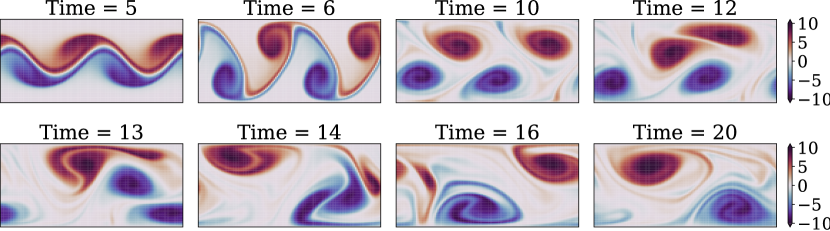
Before making this comparison, we discuss a typical vorticity evolution from the ground-truth UHR data (Figure 4). In the initial stage (), the unstable jet meanders and collapses into multiple vortices, while developing fine filaments. The vortices then merge into a flow with wavenumber 1 (), where the small-scale structure is again enhanced (). Finally, the wavenumber-1 vorticity continues to propagate westward, i.e., in the negative direction (). This final state of the coherent vortices is characteristic of the regime of mixing barriers with strong eddies and can be understood through Rossby-wave dynamics [David \BOthers. (\APACyear2017)]. All fluid simulations were terminated at (Section 4.3) because no fine-scale pattern developed in this statistically steady state.
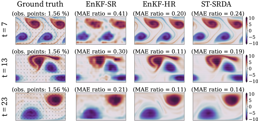
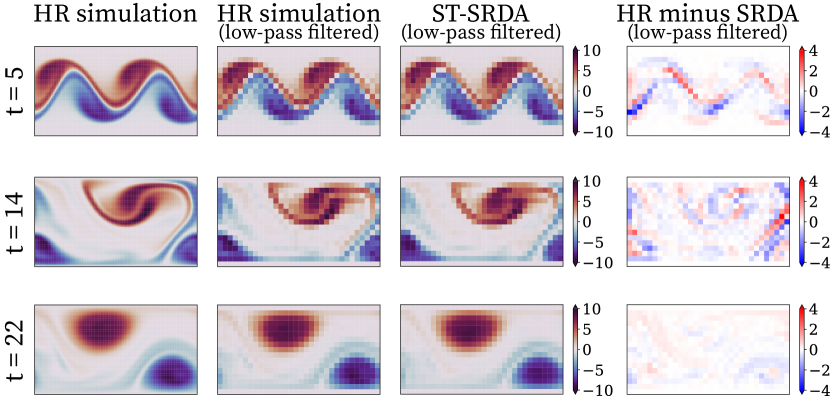
The ST-SRDA successfully inferred both the small- and large-scale structures in the vorticity fields. Figure 5 compares the ground truth with the EnKF-SR, EnKF-HR, and ST-SRDA inferences. At , the wavenumber-2 structure developed and was associated with the collapse of the jet stream (Figure 4). The ST-SRDA and EnKF-HR emulated this collapse with high accuracy; in particular, both reproduced the small-scale structures within the positive and negative vortices. Although the EnKF-SR inferred the vortex locations, it failed to reproduce the fine-scale patterns inside the vortices. At , the results were similar to those at : the vortex merging was successfully emulated by the ST-SRDA and EnKF-HR, but not by the EnKF-SR. At , the large-scale coherent vortices propagated westward, and all models successfully inferred the phase of vorticity, i.e., the large-scale pattern. Overall, the ST-SRDA inferred vorticity fields that were similar to those of the EnKF-HR.
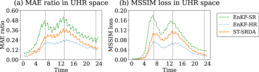
The quantitative analysis indicated that the ST-SRDA inference tended to be more accurate than the EnKF-SR inference at all time points. Figure 6 shows the time series of the MAE ratio and MSSIM loss averaged over all of the test simulations. All scores were calculated in the UHR space, with LR and HR vorticity fields mapped to the UHR space via bicubic interpolation. The results were not sensitive to this mapping because a similar time series set was obtained when all of the scores were calculated in the LR or HR space. All time series in Figure 6 are based on the analysis and forecast values of the vorticity. Since the assimilation intervals () were the same for all models, the MAE ratio and MSSIM loss were reduced at the same time points. The time series of the ST-SRDA (orange solid lines) are missing for because no forecast was inferred during this initial period (Section 4.3). On average, the MAE ratio and MSSIM loss of the ST-SRDA were smaller than those of the EnKF-SR (green dashed lines), but larger than those of the EnKF-HR (blue dotted lines). This verifies that the EnKF-HR provides a lower bound on the errors for the ST-SRDA. The time series of the EnKF-SR have two peaks around and (vertical lines). These peaks reflect the development of fine-scale patterns due to jet stream collapse () and vortex merging () (Figures 4 and 5). These two peaks are observed for the MSSIM loss of the ST-SRDA and EnKF-HR (Figure 6b), but are not clear for their MAE ratios (Figure 6a). This result is likely due to the fact that the MAE ratio is a pixel-wise error and not sensitive to differences in flow patterns [<]e.g.,¿Wang+2004IEEE. After the vortex merging (), the MAE ratio and MSSIM loss decreased, while the flow field approached the statistically steady large-scale state. This result is plausible as it is relatively easy to infer large-scale flow patterns.
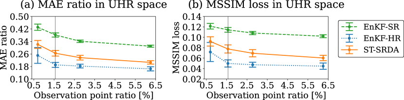
The accuracy of the ST-SRDA was comparable to that of the EnKF-HR with sparse observations. Figure 7 shows the dependence of the MAE ratio and MSSIM loss on the observation point ratio. The error bars represent the standard deviations based on all 50 test simulations. Both errors of the ST-SRDA (orange solid lines) are smaller than those of the EnKF-SR (green dashed lines), but larger than those of the EnKF-HR (blue dotted lines), as in Figure 6. For all the models, the means and standard deviations of the test scores tended to increase as observations became sparser. In particular, the error bars of the EnKF-HR were so large that they overlapped with those of the ST-SRDA at an observation point ratio of 0.69%. This implies that the accuracy of the ST-SRDA is relatively robust and becomes comparable to that of the EnKF-HR when observations are sparse.
The computation time of ST-SRDA was much shorter than that of EnKF-SR and EnKF-HR. Table 2 compares the average wall times of all the models. For reference, the table also lists the wall times of the underlying HR and LR fluid models. The wall time of the ST-SRDA was approximately 22% and 1.3% of that of the EnKF-SR and the EnKF-HR, respectively, which highlights the computational efficiency of ST-SRDA.
| Model name | Wall time [s] |
|---|---|
| HR fluid model | 696.3 |
| LR fluid model | 28.9 |
| EnKF-HR | 4415.6 |
| EnKF-SR | 262.5 |
| ST-SRDA | 57.2 |
5.2 Features for Observations Including Missing Values
In general, NNs can learn data representations suitable for specific problems [<]e.g.,¿Bengio+2013TPAMI, Zeiler+2014ECCV. Here, it is interesting to examine the representations for the observation data because of missing values. We show that the spatial range with the influence of observed grid points can increase in deeper layers.
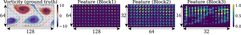
Figure 8 shows features extracted from the observation data that appear to be explainable. These features are outputs from Block 1 through 3 in Figure 3 and have smaller spatial sizes in the deeper layers due to the U-Net architecture. In these feature fields, small background values may reflect missing values, while the larger values are interpreted as representations of each observed point. The wavenumber-2 structure in the ground truth becomes more obvious in deeper-level features (Figure 8). This implies that the observed grid points may have a larger spatial influence in deeper layers.
In the fourth panel, “Feature (Block 3)” is quite low near the center, which seems to coincide with the negative vortex in the first panel (ground truth). Moreover, this feature exhibits similar low values near unobserved points. These findings suggest that the NN has difficulty distinguishing between the missing values and minimum normalized vorticity, as both are represented by zeros (Section 4.2). The differentiation can be achieved by introducing binary masks, which are frequently employed in image inpainting [<]e.g.,¿Liu+2018ECCV, Yu+2019ICCV. These masks assign to unobserved grid points and to observed points. Even if the missing and minimum observed values are the same, the binary mask enables the NN to distinguish between them. The image inpainting techniques may be beneficial for future studies.
5.3 Robustness of ST-SRDA Inferences
Here, we demonstrate that the domain shift can reduce the accuracy of ST-SRDA and SR-mixup mitigates this degradation. The domain shift occurs due to the difference in the calculation process between the test and training phases. In the test phase, the NN inference and LR fluid simulation are performed alternately, where the LR fluid model is initialized by the NN inference (Section 2.2 and Figure 2a). In contrast, during the training, the LR fluid model is initialized using the HR simulation results, and feedback from the NN to the fluid model is not incorporated (Section 2.3 and Figure 2b). We focused only on this difference in the calculation process by using the HR instead of the UHR ground truth. According to the training and test methods in Section 4.3, the observations were generated from the HR simulations during training, whereas they were generated from the UHR results during testing. Thus, both the calculation process and method of generating observations differ from those in the training phase. This experimental setup is suitable for evaluating the ST-SRDA accuracy (Section 5.1), but not for investigating the influence of domain shift. To eliminate the difference in the observations, they are generated here from the HR ground truth. The evaluation metrics (Equations 15 and 16) are then computed in the HR space. We first examined that the difference in the calculation process leads to a domain shift, namely a statistical difference in the input of LR fluid-model states.
Figure 9 shows an example of the vorticity difference between the HR simulation and ST-SRDA inference. In the training phase, the LR fluid model was initialized by the low-pass filtered HR simulation results, while in the testing phase, it was initialized by the filtered ST-SRDA inferences. The difference in the initial condition tended to be larger for the small-scale patterns associated with jet collapse () and vortex merging (), whereas the difference was smaller in the final state with large-scale vortices (). We also confirmed that the probability density functions of vorticity values varied significantly in terms of the Kolmogorov-Smirnov test, where the p-value was less than . These results indicate that the difference in the initial condition was significant, implying that the obtained LR time series was also statistically different between the training and test phases, i.e., a domain shift occurred.
We next investigated the influence of the domain shift. For comparison, the NN was trained without SR-mixup. Note that all results presented in Sections 5.1 and 5.2 employed SR-mixup. The NNs with and without SR-mixup were compared using the two evaluation methods illustrated in Figure 2. The first method (Figure 2a) is the same as the test method in Section 5.1, where the domain shift occurred. In contrast, in the second method (Figure 2b), the domain shift does not occur because it is the same as the method used to generate the training data. In this method, there is no feedback from the NN inference to the LR simulation.
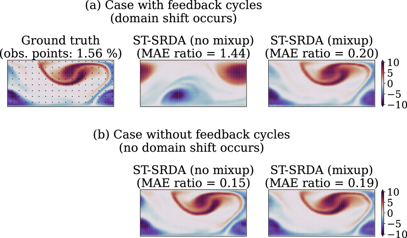
The domain shift potentially reduces ST-SRDA performance, but SR-mixup can mitigate this effect. Figure 10 shows vorticity snapshots obtained using the two evaluation methods. Without SR-mixup, the vorticity was accurately inferred (MAE ratio ) when no domain shift occurred (Figure 10b). However, when the feedback was incorporated, i.e., the domain shift occurred (Figure 10a), the vortex shapes were completely different from those in the ground truth, resulting in a higher MAE ratio (). In contrast, when SR-mixup was employed, the inferences were not strongly dependent on the presence or absence of the domain shift (Figures 10a and 10b, respectively). These results indicate that SR-mixup makes the inference robust to statistical differences in the input.
The effect of SR-mixup was further examined by varying the observation point ratio (Figure 11). Without SR-mixup, the MAE ratio was substantially higher over the entire range of the observation point ratio when the domain shift occurred (dashed line in Figure 11a). In contrast, using SR-mixup, the increase in the MAE ratio was suppressed, and the MAE ratio was almost independent of the domain shift (solid lines in Figures 11a and 11b). Interestingly, when the feedback was not incorporated (Figure 11b), the MAE ratio was slightly higher with SR-mixup than without SR-mixup. During the training phase, SR-mixup added perturbations to the LR input (Equation 4.3), whereas in the evaluation for Figure 11b, such perturbations were not added, and the LR initial condition was generated directly from the HR data. Thus, the training without SR-mixup resulted in smaller MAE ratios. However, this evaluation method is virtual because the LR fluid model is always initialized by the HR data; the inclusion of the feedback cycle is more realistic (Figure 11a).
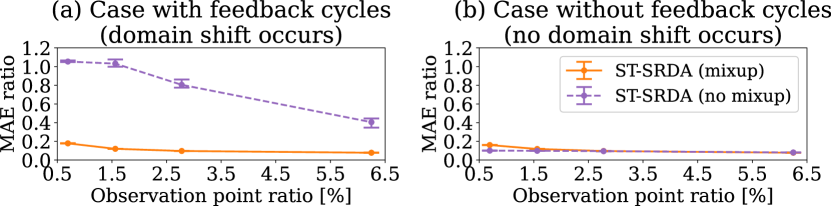
Furthermore, SR-mixup reduced the sensitivity of inference to the NN-weight initialization, as shown by the error bars in Figure 11. In general, the NN inference can be influenced by randomly initialized weights [<]e.g.,¿Bengio2012, Picard2021arXiv. To assess this sensitivity, we trained the NN five times while changing the random seed for the weight initializer [He \BOthers. (\APACyear2015)]. The error bars in the figure show the maxima and minima of the MAE ratios from these five experiments. When the domain shift did not occur, the error bars were quite small, regardless of SR-mixup (Figure 11b). In contrast, when the domain shift occurred, the error bars were significantly larger without SR-mixup (dashed line in Figure 11a). Therefore, SR-mixup suppressed the sensitivity and promoted the stability of the inference.
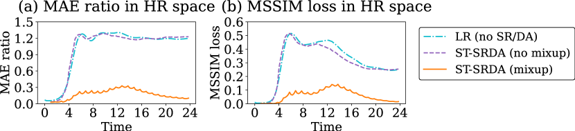
The MAE ratio without SR-mixup was saturated at an observation point ratio of 0.56%, resulting in the small error bar (purple) in Figure 11a. For comparison, we conducted the LR fluid simulation without DA or SR, which was expected to give an upper error bound for the ST-SRDA. Figure 12 compares the time series of the MAE ratio when the observation point ratio is 0.56%. As expected, the MAE ratio of the ST-SRDA without SR-mixup was comparable to that of the LR simulation, both of which were much larger than that of the ST-SRDA with SR-mixup. In particular, the error grew rapidly in the initial period (). Similar error growth was observed at the other observation point ratios, i.e., with denser observations. During the initial period, the jet stream collapses while developing fine-scale vorticity filaments (Figure 4), which can enhance the domain shift (Figure 9). This could explain the rapid error growth without SR-mixup found in Figure 12.
Finally, we discuss three possible reasons why domain-generalization techniques have rarely been applied to fluid systems, including the atmosphere and ocean [Brunton \BOthers. (\APACyear2020), Duraisamy (\APACyear2021), Kashinath \BOthers. (\APACyear2021)]. First, despite the reduced accuracy due to domain shift, the NN inference can remain more accurate than that of baselines, making domain-generalization methods less necessary. Second, loss functions that include physics-based terms, such as the residuals of the governing equations, can act as regularizers that improve generalizability [<]e.g.,¿Jiang+2020ICHPC, Wang+2020NIPS, Bao+2022CUAI, Hammoud+2022JAMES. Third, incorporating geometric symmetries as prior knowledge can enhance the generalization performance [<]e.g.,¿Ling2016JFM, Wang2021ICLR, Chattopadhyay+2022GMDD, Yasuda+2023APLML. Further research is needed to evaluate the validity of these factors. As we have demonstrated, domain shifts can occur when NNs are incorporated into physics-based models, thereby reducing accuracy. By utilizing domain-generalization techniques [<]e.g.,¿Wang+2022IEEE, Zhou+2022IEEE, even in the three cases described here, it may be possible to further improve the robustness of NNs and extend their applicability to different systems.
6 Conclusions
This study proposes a four-dimensional super-resolution data assimilation (4D-SRDA) scheme. This scheme employs a physics-based model to calculate the time evolution of a system using low-resolution (LR) simulations. The resulting time series of LR model states, along with observations, are fed into a trained neural network (NN). This NN simultaneously performs data assimilation (DA) and spatio-temporal super-resolution (SR), generating flow fields with high spatio-temporal resolution. A snapshot of these high-resolution (HR) flow fields is considered the analysis and projected onto the LR grid points via algebraic operations, such as linear interpolation. Using this LR analysis, an LR simulation is conducted for the next assimilation cycle. 4D-SRDA does not require ensemble evolution or iterative calculations, making it computationally efficient.
In the 4D-SRDA system, the NN is trained via supervised or unsupervised learning, in which a domain shift, namely a statistical difference between the training and test data, can affect the performance of the system [<]e.g.,¿MorenoTorres+2012PR. In general, when physics-based simulations and NN inferences are performed alternately and are mutually dependent in the test phase, a domain shift will occur if the training data are generated in advance solely by running the physics-based model (i.e., offline training).
To prevent the degradation in accuracy caused by the domain shift, we developed a data augmentation method for domain generalization, SR-mixup, based on C-Mixup [Yao \BOthers. (\APACyear2022)]. In SR-mixup, two similar inputs are randomly sampled and their linear combination is used as input to improve robustness to domain shift. Unlike C-Mixup, the linear combination is not made for the output, to avoid producing blurred HR images in SR problems. SR-mixup is applicable to supervised and unsupervised problems because it does not assume paired inputs and outputs.
We validated the 4D-SRDA and SR-mixup using an idealized barotropic ocean jet [David \BOthers. (\APACyear2017)] with supervised learning. Since this jet was modeled as a two-dimensional flow, 4D-SRDA was referred to as spatio-temporal SRDA (ST-SRDA). In the case of supervised learning, the ST-SRDA is regarded as a computationally efficient surrogate scheme for generating an HR reanalysis dataset. For comparison, we applied an ensemble Kalman filter (EnKF) to the LR or HR fluid model. The former is a baseline model for the ST-SRDA, while the latter is considered to give a lower error bound for the ST-SRDA because the underlying HR fluid model generates the HR training data. The ST-SRDA always tended to be more accurate than the baseline, i.e., the EnKF at the LR. When the observations were sparse, the error of the ST-SRDA became comparable to that of the EnKF at the HR (i.e., close to a lower error bound). Furthermore, the wall time of ST-SRDA was much shorter than that of the EnKFs. These results suggest that ST-SRDA is effective for generating HR reanalysis at low computational cost. We also confirmed that the error became substantially larger without SR-mixup, indicating that the combination of SR-mixup and ST-SRDA is useful in achieving robust forecast cycles.
To improve the applicability of this scheme to real-world contexts, a training method using small patches should be developed. In this study, the NN was trained based on the whole two-dimensional flow fields. The data size of three-dimensional flows is larger, which requires the division of a snapshot into small patches. Training methods with small patches have been developed in terms of DA [Ouala \BOthers. (\APACyear2018), Yang \BBA Grooms (\APACyear2021)] and may be effective in applying 4D-SRDA to more realistic three-dimensional data.
Another direction for future work is to achieve 4D-SRDA with unsupervised learning. The proof-of-concept presented here employed supervised learning, assuming that sufficiently accurate atmospheric or oceanic data were available in the training phase. In practice, such data can be obtained from HR reanalysis datasets. Unsupervised settings will make 4D-SRDA applicable to a broader range of conditions, in which accurate data may not be available. Furthermore, since 4D-SRDA does not require ensembles, it is difficult to estimate the uncertainty of the inferences. This may be improved by utilizing unsupervised-learning frameworks [<]e.g.,¿Krishnan+2015arXiv, Fraccaro+2017NIPS. Although the numerical experiments in this paper are idealized, the super-resolution and domain-generalization techniques presented herein provide a useful basis for future developments in the integration of data-driven and physics-based models.
Appendix A Hyperparameters of the Neural Network
We list here the hyperparameters of the NN (Figure 3), which were determined through a grid search. Further details about the implementation are available at the Zenodo repository (see Open Research). Tables 3 and 4 list the layer-dependent hyperparameters in the encoder and decoder, respectively. The kernel size of all convolution layers is . The slope of all leaky ReLU layers is [Maas \BOthers. (\APACyear2013)]. The upscale factor of all pixel shuffle layers is [Shi \BOthers. (\APACyear2016)]. The hyperparameters in the transformer encoding blocks are set as follows [Vaswani \BOthers. (\APACyear2017)]: the number of input features is , the number of heads in the multi-head attention is , and the dimension of the feed-forward network is .
| Block name | Layer name | Input channels | Output channels | Stride |
|---|---|---|---|---|
| — | Conv2D-1 | 1 | 64 | 1 |
| Downsample-1 | Conv2D-2 | 64 | 128 | 2 |
| Conv2D-3 | 128 | 128 | 1 | |
| Downsample-2 | Conv2D-2 | 128 | 256 | 2 |
| Conv2D-3 | 256 | 256 | 1 | |
| Downsample-3 | Conv2D-2 | 256 | 128 | 2 |
| Conv2D-3 | 128 | 128 | 1 | |
| Downsample-4 | Conv2D-2 | 128 | 64 | 2 |
| Conv2D-3 | 64 | 64 | 1 |
| Block name | Layer name | Input channels | Output channels |
|---|---|---|---|
| Upsample-1 | Conv2D-4 | 64 | 256 |
| Conv2D-5 | 64 | 128 | |
| Upsample-2 | Conv2D-4 | 128 | 512 |
| Conv2D-5 | 128 | 256 | |
| Upsample-3 | Conv2D-4 | 256 | 1024 |
| Conv2D-5 | 256 | 128 | |
| Upsample-4 | Conv2D-4 | 128 | 512 |
| Conv2D-5 | 128 | 64 | |
| — | Conv2D-6 | 192 | 64 |
| Conv2D-7 | 64 | 1 |
Open Research
The source code used for generating all the datasets and experiments is preserved at https://doi.org/10.5281/zenodo.7946486 and developed openly at https://github.com/YukiYasuda2718/4d-srda_sr-mixup. The detailed information can be found in \citeAYasuda+2023ZenodoSrdaMixup.
Acknowledgements.
We greatly appreciate the three anonymous reviewers, the associate editor, and the editor for their careful review and constructive feedback on the manuscript. This work was supported by the JSPS KAKENHI (Grant Number 20H05751). This work used computational resources of the TSUBAME3.0 supercomputer provided by the Tokyo Institute of Technology through the HPCI System Research Project (Project ID: hp220102). This paper is based on results obtained from a project, JPNP22002, commissioned by the New Energy and Industrial Technology Development Organization (NEDO).References
- Abarbanel \BOthers. (\APACyear2018) \APACinsertmetastarAbarbanel+2018NC{APACrefauthors}Abarbanel, H\BPBID\BPBII., Rozdeba, P\BPBIJ.\BCBL \BBA Shirman, S. \APACrefYearMonthDay201808. \BBOQ\APACrefatitleMachine Learning: Deepest Learning as Statistical Data Assimilation Problems Machine Learning: Deepest Learning as Statistical Data Assimilation Problems.\BBCQ \APACjournalVolNumPagesNeural Computation3082025-2055. {APACrefURL} https://doi.org/10.1162/neco\_a\_01094 {APACrefDOI} 10.1162/neco_a_01094 \PrintBackRefs\CurrentBib
- Amendola \BOthers. (\APACyear2021) \APACinsertmetastarAmendola+2021{APACrefauthors}Amendola, M., Arcucci, R., Mottet, L., Casas, C\BPBIQ., Fan, S., Pain, C.\BDBLGuo, Y\BHBIK. \APACrefYearMonthDay2021. \BBOQ\APACrefatitleData Assimilation in the Latent Space of a Convolutional Autoencoder Data assimilation in the latent space of a convolutional autoencoder.\BBCQ \BIn \APACrefbtitleComputational Science – ICCS 2021: 21st International Conference, Krakow, Poland, June 16–18, 2021, Proceedings, Part V Computational science – iccs 2021: 21st international conference, krakow, poland, june 16–18, 2021, proceedings, part v (\BPG 373–386). \APACaddressPublisherBerlin, HeidelbergSpringer-Verlag. {APACrefURL} https://doi.org/10.1007/978-3-030-77977-1_30 {APACrefDOI} 10.1007/978-3-030-77977-1_30 \PrintBackRefs\CurrentBib
- Anderson \BBA Anderson (\APACyear1999) \APACinsertmetastarAnderson+1999{APACrefauthors}Anderson, J\BPBIL.\BCBT \BBA Anderson, S\BPBIL. \APACrefYearMonthDay1999. \BBOQ\APACrefatitleA Monte Carlo Implementation of the Nonlinear Filtering Problem to Produce Ensemble Assimilations and Forecasts A monte carlo implementation of the nonlinear filtering problem to produce ensemble assimilations and forecasts.\BBCQ \APACjournalVolNumPagesMonthly Weather Review127122741 - 2758. {APACrefURL} https://journals.ametsoc.org/view/journals/mwre/127/12/1520-0493_1999_127_2741_amciot_2.0.co_2.xml {APACrefDOI} 10.1175/1520-0493(1999)127¡2741:AMCIOT¿2.0.CO;2 \PrintBackRefs\CurrentBib
- Anwar \BOthers. (\APACyear2020) \APACinsertmetastarAnwar+2020ACMCS{APACrefauthors}Anwar, S., Khan, S.\BCBL \BBA Barnes, N. \APACrefYearMonthDay2020may. \BBOQ\APACrefatitleA Deep Journey into Super-Resolution: A Survey A deep journey into super-resolution: A survey.\BBCQ \APACjournalVolNumPagesACM Comput. Surv.533. {APACrefURL} https://doi.org/10.1145/3390462 {APACrefDOI} 10.1145/3390462 \PrintBackRefs\CurrentBib
- Asch \BOthers. (\APACyear2016) \APACinsertmetastarAsch+2016SIAM{APACrefauthors}Asch, M., Bocquet, M.\BCBL \BBA Nodet, M. \APACrefYear2016. \APACrefbtitleData Assimilation Data assimilation. \APACaddressPublisherPhiladelphia, PASociety for Industrial and Applied Mathematics. {APACrefURL} https://epubs.siam.org/doi/abs/10.1137/1.9781611974546 {APACrefDOI} 10.1137/1.9781611974546 \PrintBackRefs\CurrentBib
- Bao \BOthers. (\APACyear2022) \APACinsertmetastarBao+2022CUAI{APACrefauthors}Bao, T., Chen, S., Johnson, T\BPBIT., Givi, P., Sammak, S.\BCBL \BBA Jia, X. \APACrefYearMonthDay2022. \BBOQ\APACrefatitlePhysics Guided Neural Networks for Spatio-temporal Super-resolution of Turbulent Flows Physics guided neural networks for spatio-temporal super-resolution of turbulent flows.\BBCQ \BIn \APACrefbtitleThe 38th Conference on Uncertainty in Artificial Intelligence. The 38th conference on uncertainty in artificial intelligence. {APACrefURL} https://openreview.net/forum?id=S98VJL8jcxq \PrintBackRefs\CurrentBib
- Barthélémy \BOthers. (\APACyear2022) \APACinsertmetastarBarthelemy+2022OD{APACrefauthors}Barthélémy, S., Brajard, J., Bertino, L.\BCBL \BBA Counillon, F. \APACrefYearMonthDay20228. \BBOQ\APACrefatitleSuper-resolution data assimilation Super-resolution data assimilation.\BBCQ \APACjournalVolNumPagesOcean Dynamics72661-678. {APACrefDOI} 10.1007/s10236-022-01523-x \PrintBackRefs\CurrentBib
- Beauchamp \BOthers. (\APACyear2022) \APACinsertmetastarBeauchamp+2022GMDD{APACrefauthors}Beauchamp, M., Febvre, Q., Georgenthum, H.\BCBL \BBA Fablet, R. \APACrefYearMonthDay2022. \BBOQ\APACrefatitle4DVarNet-SSH: end-to-end learning of variational interpolation schemes for nadir and wide-swath satellite altimetry 4dvarnet-ssh: end-to-end learning of variational interpolation schemes for nadir and wide-swath satellite altimetry.\BBCQ \APACjournalVolNumPagesGeoscientific Model Development Discussions20221–37. {APACrefURL} https://gmd.copernicus.org/preprints/gmd-2022-241/ {APACrefDOI} 10.5194/gmd-2022-241 \PrintBackRefs\CurrentBib
- Bengio (\APACyear2012) \APACinsertmetastarBengio2012{APACrefauthors}Bengio, Y. \APACrefYearMonthDay2012. \BBOQ\APACrefatitlePractical Recommendations for Gradient-Based Training of Deep Architectures Practical recommendations for gradient-based training of deep architectures.\BBCQ \BIn G. Montavon, G\BPBIB. Orr\BCBL \BBA K\BHBIR. Müller (\BEDS), \APACrefbtitleNeural Networks: Tricks of the Trade: Second Edition Neural networks: Tricks of the trade: Second edition (\BPGS 437–478). \APACaddressPublisherBerlin, HeidelbergSpringer Berlin Heidelberg. {APACrefURL} https://doi.org/10.1007/978-3-642-35289-8_26 {APACrefDOI} 10.1007/978-3-642-35289-8_26 \PrintBackRefs\CurrentBib
- Bengio \BOthers. (\APACyear2013) \APACinsertmetastarBengio+2013TPAMI{APACrefauthors}Bengio, Y., Courville, A.\BCBL \BBA Vincent, P. \APACrefYearMonthDay2013. \BBOQ\APACrefatitleRepresentation Learning: A Review and New Perspectives Representation learning: A review and new perspectives.\BBCQ \APACjournalVolNumPagesIEEE Transactions on Pattern Analysis and Machine Intelligence3581798-1828. {APACrefDOI} 10.1109/TPAMI.2013.50 \PrintBackRefs\CurrentBib
- Brunton \BOthers. (\APACyear2020) \APACinsertmetastarBrunton+2020ARFM{APACrefauthors}Brunton, S\BPBIL., Noack, B\BPBIR.\BCBL \BBA Koumoutsakos, P. \APACrefYearMonthDay2020. \BBOQ\APACrefatitleMachine Learning for Fluid Mechanics Machine learning for fluid mechanics.\BBCQ \APACjournalVolNumPagesAnnual Review of Fluid Mechanics521477-508. {APACrefURL} https://doi.org/10.1146/annurev-fluid-010719-060214 {APACrefDOI} 10.1146/annurev-fluid-010719-060214 \PrintBackRefs\CurrentBib
- Burgers \BOthers. (\APACyear1998) \APACinsertmetastarBurgers+1998MWR{APACrefauthors}Burgers, G., van Leeuwen, P\BPBIJ.\BCBL \BBA Evensen, G. \APACrefYearMonthDay1998. \BBOQ\APACrefatitleAnalysis Scheme in the Ensemble Kalman Filter Analysis scheme in the ensemble kalman filter.\BBCQ \APACjournalVolNumPagesMonthly Weather Review12661719 - 1724. {APACrefURL} https://journals.ametsoc.org/view/journals/mwre/126/6/1520-0493_1998_126_1719_asitek_2.0.co_2.xml {APACrefDOI} 10.1175/1520-0493(1998)126¡1719:ASITEK¿2.0.CO;2 \PrintBackRefs\CurrentBib
- Chattopadhyay \BOthers. (\APACyear2022) \APACinsertmetastarChattopadhyay+2022GMDD{APACrefauthors}Chattopadhyay, A., Mustafa, M., Hassanzadeh, P., Bach, E.\BCBL \BBA Kashinath, K. \APACrefYearMonthDay2022. \BBOQ\APACrefatitleTowards physics-inspired data-driven weather forecasting: integrating data assimilation with a deep spatial-transformer-based U-NET in a case study with ERA5 Towards physics-inspired data-driven weather forecasting: integrating data assimilation with a deep spatial-transformer-based u-net in a case study with era5.\BBCQ \APACjournalVolNumPagesGeoscientific Model Development1552221–2237. {APACrefURL} https://gmd.copernicus.org/articles/15/2221/2022/ {APACrefDOI} 10.5194/gmd-15-2221-2022 \PrintBackRefs\CurrentBib
- Chen \BOthers. (\APACyear2018) \APACinsertmetastarChen+2018NIPS{APACrefauthors}Chen, R\BPBIT\BPBIQ., Rubanova, Y., Bettencourt, J.\BCBL \BBA Duvenaud, D. \APACrefYearMonthDay2018. \BBOQ\APACrefatitleNeural Ordinary Differential Equations Neural ordinary differential equations.\BBCQ \BIn \APACrefbtitleProceedings of the 32nd International Conference on Neural Information Processing Systems Proceedings of the 32nd international conference on neural information processing systems (\BPG 6572–6583). \APACaddressPublisherRed Hook, NY, USACurran Associates Inc. \PrintBackRefs\CurrentBib
- Cheng \BOthers. (\APACyear2023) \APACinsertmetastarCheng+2023arXiv{APACrefauthors}Cheng, S., Quilodran-Casas, C., Ouala, S., Farchi, A., Liu, C., Tandeo, P.\BDBLArcucci, R. \APACrefYearMonthDay2023. \APACrefbtitleMachine learning with data assimilation and uncertainty quantification for dynamical systems: a review. Machine learning with data assimilation and uncertainty quantification for dynamical systems: a review. \PrintBackRefs\CurrentBib
- Cohen \BOthers. (\APACyear2019) \APACinsertmetastarCohen+2019NIPS{APACrefauthors}Cohen, T\BPBIS., Geiger, M.\BCBL \BBA Weiler, M. \APACrefYearMonthDay2019. \BBOQ\APACrefatitleA General Theory of Equivariant CNNs on Homogeneous Spaces A general theory of equivariant cnns on homogeneous spaces.\BBCQ \BIn H. Wallach, H. Larochelle, A. Beygelzimer, F. d'Alché-Buc, E. Fox\BCBL \BBA R. Garnett (\BEDS), \APACrefbtitleAdvances in Neural Information Processing Systems Advances in neural information processing systems (\BVOL 32). \APACaddressPublisherCurran Associates, Inc. {APACrefURL} https://proceedings.neurips.cc/paper_files/paper/2019/file/b9cfe8b6042cf759dc4c0cccb27a6737-Paper.pdf \PrintBackRefs\CurrentBib
- David \BOthers. (\APACyear2017) \APACinsertmetastarDavid+2017OM{APACrefauthors}David, T\BPBIW., Marshall, D\BPBIP.\BCBL \BBA Zanna, L. \APACrefYearMonthDay2017. \BBOQ\APACrefatitleThe statistical nature of turbulent barotropic ocean jets The statistical nature of turbulent barotropic ocean jets.\BBCQ \APACjournalVolNumPagesOcean Modelling11334-49. {APACrefURL} https://www.sciencedirect.com/science/article/pii/S1463500317300392 {APACrefDOI} https://doi.org/10.1016/j.ocemod.2017.03.008 \PrintBackRefs\CurrentBib
- Dong \BOthers. (\APACyear2014) \APACinsertmetastarDong+2014ECCV{APACrefauthors}Dong, C., Loy, C\BPBIC., He, K.\BCBL \BBA Tang, X. \APACrefYearMonthDay2014. \BBOQ\APACrefatitleLearning a Deep Convolutional Network for Image Super-Resolution Learning a deep convolutional network for image super-resolution.\BBCQ \BIn D. Fleet, T. Pajdla, B. Schiele\BCBL \BBA T. Tuytelaars (\BEDS), \APACrefbtitleComputer Vision – ECCV 2014 Computer vision – eccv 2014 (\BPGS 184–199). \APACaddressPublisherChamSpringer International Publishing. \PrintBackRefs\CurrentBib
- Ducournau \BBA Fablet (\APACyear2016) \APACinsertmetastarDucournau+2016PRRS{APACrefauthors}Ducournau, A.\BCBT \BBA Fablet, R. \APACrefYearMonthDay2016. \BBOQ\APACrefatitleDeep learning for ocean remote sensing: an application of convolutional neural networks for super-resolution on satellite-derived SST data Deep learning for ocean remote sensing: an application of convolutional neural networks for super-resolution on satellite-derived sst data.\BBCQ \BIn (\BPG 1-6). {APACrefDOI} 10.1109/PRRS.2016.7867019 \PrintBackRefs\CurrentBib
- Duraisamy (\APACyear2021) \APACinsertmetastarDuraisamy2021PRF{APACrefauthors}Duraisamy, K. \APACrefYearMonthDay2021May. \BBOQ\APACrefatitlePerspectives on machine learning-augmented Reynolds-averaged and large eddy simulation models of turbulence Perspectives on machine learning-augmented reynolds-averaged and large eddy simulation models of turbulence.\BBCQ \APACjournalVolNumPagesPhys. Rev. Fluids6050504. {APACrefURL} https://link.aps.org/doi/10.1103/PhysRevFluids.6.050504 {APACrefDOI} 10.1103/PhysRevFluids.6.050504 \PrintBackRefs\CurrentBib
- Evensen (\APACyear1994) \APACinsertmetastarEvensen1994JGRO{APACrefauthors}Evensen, G. \APACrefYearMonthDay1994. \BBOQ\APACrefatitleSequential data assimilation with a nonlinear quasi-geostrophic model using Monte Carlo methods to forecast error statistics Sequential data assimilation with a nonlinear quasi-geostrophic model using monte carlo methods to forecast error statistics.\BBCQ \APACjournalVolNumPagesJournal of Geophysical Research: Oceans99C510143-10162. {APACrefURL} https://agupubs.onlinelibrary.wiley.com/doi/abs/10.1029/94JC00572 {APACrefDOI} https://doi.org/10.1029/94JC00572 \PrintBackRefs\CurrentBib
- Fablet \BOthers. (\APACyear2021) \APACinsertmetastarFablet+2021{APACrefauthors}Fablet, R., Chapron, B., Drumetz, L., Mémin, E., Pannekoucke, O.\BCBL \BBA Rousseau, F. \APACrefYearMonthDay2021. \BBOQ\APACrefatitleLearning Variational Data Assimilation Models and Solvers Learning variational data assimilation models and solvers.\BBCQ \APACjournalVolNumPagesJournal of Advances in Modeling Earth Systems1310e2021MS002572. {APACrefURL} https://agupubs.onlinelibrary.wiley.com/doi/abs/10.1029/2021MS002572 \APACrefnotee2021MS002572 2021MS002572 {APACrefDOI} https://doi.org/10.1029/2021MS002572 \PrintBackRefs\CurrentBib
- Fraccaro \BOthers. (\APACyear2017) \APACinsertmetastarFraccaro+2017NIPS{APACrefauthors}Fraccaro, M., Kamronn, S., Paquet, U.\BCBL \BBA Winther, O. \APACrefYearMonthDay2017. \BBOQ\APACrefatitleA Disentangled Recognition and Nonlinear Dynamics Model for Unsupervised Learning A disentangled recognition and nonlinear dynamics model for unsupervised learning.\BBCQ \BIn \APACrefbtitleNIPS Nips (\BPG 3604-3613). {APACrefURL} http://papers.nips.cc/paper/6951-a-disentangled-recognition-and-nonlinear-dynamics-model-for-unsupervised-learning \PrintBackRefs\CurrentBib
- Fuchs \BOthers. (\APACyear2020) \APACinsertmetastarFuchs2020{APACrefauthors}Fuchs, F., Worrall, D., Fischer, V.\BCBL \BBA Welling, M. \APACrefYearMonthDay2020. \BBOQ\APACrefatitleSE(3)-Transformers: 3D Roto-Translation Equivariant Attention Networks Se(3)-transformers: 3d roto-translation equivariant attention networks.\BBCQ \BIn H. Larochelle, M. Ranzato, R. Hadsell, M\BPBIF. Balcan\BCBL \BBA H. Lin (\BEDS), \APACrefbtitleAdvances in Neural Information Processing Systems Advances in neural information processing systems (\BVOL 33, \BPGS 1970–1981). \APACaddressPublisherCurran Associates, Inc. {APACrefURL} https://proceedings.neurips.cc/paper/2020/file/15231a7ce4ba789d13b722cc5c955834-Paper.pdf \PrintBackRefs\CurrentBib
- Gaspari \BBA Cohn (\APACyear1999) \APACinsertmetastarGaspari+1999QJRMS{APACrefauthors}Gaspari, G.\BCBT \BBA Cohn, S\BPBIE. \APACrefYearMonthDay1999. \BBOQ\APACrefatitleConstruction of correlation functions in two and three dimensions Construction of correlation functions in two and three dimensions.\BBCQ \APACjournalVolNumPagesQuarterly Journal of the Royal Meteorological Society125554723-757. {APACrefURL} https://rmets.onlinelibrary.wiley.com/doi/abs/10.1002/qj.49712555417 {APACrefDOI} https://doi.org/10.1002/qj.49712555417 \PrintBackRefs\CurrentBib
- Grooms (\APACyear2021) \APACinsertmetastarGroom2021QJRMS{APACrefauthors}Grooms, I. \APACrefYearMonthDay2021. \BBOQ\APACrefatitleAnalog ensemble data assimilation and a method for constructing analogs with variational autoencoders Analog ensemble data assimilation and a method for constructing analogs with variational autoencoders.\BBCQ \APACjournalVolNumPagesQuarterly Journal of the Royal Meteorological Society147734139-149. {APACrefURL} https://rmets.onlinelibrary.wiley.com/doi/abs/10.1002/qj.3910 {APACrefDOI} https://doi.org/10.1002/qj.3910 \PrintBackRefs\CurrentBib
- Ha \BOthers. (\APACyear2019) \APACinsertmetastarHa+2019{APACrefauthors}Ha, V\BPBIK., Ren, J\BHBIC., Xu, X\BHBIY., Zhao, S., Xie, G., Masero, V.\BCBL \BBA Hussain, A. \APACrefYearMonthDay2019. \BBOQ\APACrefatitleDeep Learning Based Single Image Super-resolution: A Survey Deep learning based single image super-resolution: A survey.\BBCQ \APACjournalVolNumPagesInternational Journal of Automation and Computing. {APACrefDOI} 10.1007/s11633-019-1183-x \PrintBackRefs\CurrentBib
- Hammoud \BOthers. (\APACyear2022) \APACinsertmetastarHammoud+2022JAMES{APACrefauthors}Hammoud, M\BPBIA\BPBIE\BPBIR., Titi, E\BPBIS., Hoteit, I.\BCBL \BBA Knio, O. \APACrefYearMonthDay2022. \BBOQ\APACrefatitleCDAnet: A Physics-Informed Deep Neural Network for Downscaling Fluid Flows Cdanet: A physics-informed deep neural network for downscaling fluid flows.\BBCQ \APACjournalVolNumPagesJournal of Advances in Modeling Earth Systems1412e2022MS003051. {APACrefURL} https://agupubs.onlinelibrary.wiley.com/doi/abs/10.1029/2022MS003051 \APACrefnotee2022MS003051 2022MS003051 {APACrefDOI} https://doi.org/10.1029/2022MS003051 \PrintBackRefs\CurrentBib
- He \BOthers. (\APACyear2015) \APACinsertmetastarHe+2015ICCV{APACrefauthors}He, K., Zhang, X., Ren, S.\BCBL \BBA Sun, J. \APACrefYearMonthDay2015December. \BBOQ\APACrefatitleDelving Deep into Rectifiers: Surpassing Human-Level Performance on ImageNet Classification Delving deep into rectifiers: Surpassing human-level performance on imagenet classification.\BBCQ \BIn \APACrefbtitleProceedings of the IEEE International Conference on Computer Vision (ICCV). Proceedings of the ieee international conference on computer vision (iccv). \PrintBackRefs\CurrentBib
- Jiang \BOthers. (\APACyear2020) \APACinsertmetastarJiang+2020ICHPC{APACrefauthors}Jiang, C., Esmaeilzadeh, S., Azizzadenesheli, K., Kashinath, K., Mustafa, M., Tchelepi, H\BPBIA.\BDBLAnandkumar, A. \APACrefYearMonthDay2020nov. \BBOQ\APACrefatitleMESHFREEFLOWNET: A Physics-Constrained Deep Continuous Space-Time Super-Resolution Framework Meshfreeflownet: A physics-constrained deep continuous space-time super-resolution framework.\BBCQ \BIn \APACrefbtitle2020 SC20: International Conference for High Performance Computing, Networking, Storage and Analysis (SC) 2020 sc20: International conference for high performance computing, networking, storage and analysis (sc) (\BPG 1-15). \APACaddressPublisherLos Alamitos, CA, USAIEEE Computer Society. {APACrefURL} https://doi.ieeecomputersociety.org/10.1109/SC41405.2020.00013 {APACrefDOI} 10.1109/SC41405.2020.00013 \PrintBackRefs\CurrentBib
- Kashinath \BOthers. (\APACyear2021) \APACinsertmetastarKashinath+2021PTRS{APACrefauthors}Kashinath, K., Mustafa, M., Albert, A., Wu, J\BHBIL., Jiang, C., Esmaeilzadeh, S.\BDBLPrabhat, n. \APACrefYearMonthDay2021. \BBOQ\APACrefatitlePhysics-informed machine learning: case studies for weather and climate modelling Physics-informed machine learning: case studies for weather and climate modelling.\BBCQ \APACjournalVolNumPagesPhilosophical Transactions of the Royal Society A: Mathematical, Physical and Engineering Sciences379219420200093. {APACrefURL} https://royalsocietypublishing.org/doi/abs/10.1098/rsta.2020.0093 {APACrefDOI} 10.1098/rsta.2020.0093 \PrintBackRefs\CurrentBib
- Kingma \BBA Ba (\APACyear2015) \APACinsertmetastarKingma+2015ICLR{APACrefauthors}Kingma, D\BPBIP.\BCBT \BBA Ba, J. \APACrefYearMonthDay2015. \BBOQ\APACrefatitleAdam: A Method for Stochastic Optimization Adam: A method for stochastic optimization.\BBCQ \BIn Y. Bengio \BBA Y. LeCun (\BEDS), . {APACrefURL} http://arxiv.org/abs/1412.6980 \PrintBackRefs\CurrentBib
- Krasnopolsky \BBA Belochitski (\APACyear2020) \APACinsertmetastarKrasnopolsky+2020arXiv{APACrefauthors}Krasnopolsky, V.\BCBT \BBA Belochitski, A\BPBIA. \APACrefYearMonthDay2020. \APACrefbtitleUsing Machine Learning for Model Physics: an Overview. Using machine learning for model physics: an overview. \APACaddressPublisherarXiv. {APACrefURL} https://arxiv.org/abs/2002.00416 {APACrefDOI} 10.48550/ARXIV.2002.00416 \PrintBackRefs\CurrentBib
- Krishnan \BOthers. (\APACyear2015) \APACinsertmetastarKrishnan+2015arXiv{APACrefauthors}Krishnan, R\BPBIG., Shalit, U.\BCBL \BBA Sontag, D. \APACrefYearMonthDay2015. \APACrefbtitleDeep Kalman Filters. Deep kalman filters. \APACaddressPublisherarXiv. {APACrefURL} https://arxiv.org/abs/1511.05121 {APACrefDOI} 10.48550/ARXIV.1511.05121 \PrintBackRefs\CurrentBib
- Li \BOthers. (\APACyear2020) \APACinsertmetastarLi+2020IEEE{APACrefauthors}Li, B., Zhang, Y., Zhao, B.\BCBL \BBA Shao, H. \APACrefYearMonthDay2020. \BBOQ\APACrefatitle3D-ReConstnet: A Single-View 3D-Object Point Cloud Reconstruction Network 3d-reconstnet: A single-view 3d-object point cloud reconstruction network.\BBCQ \APACjournalVolNumPagesIEEE Access883782-83790. {APACrefDOI} 10.1109/ACCESS.2020.2992554 \PrintBackRefs\CurrentBib
- Ling \BOthers. (\APACyear2016) \APACinsertmetastarLing2016JFM{APACrefauthors}Ling, J., Kurzawski, A.\BCBL \BBA Templeton, J. \APACrefYearMonthDay2016. \BBOQ\APACrefatitleReynolds averaged turbulence modelling using deep neural networks with embedded invariance Reynolds averaged turbulence modelling using deep neural networks with embedded invariance.\BBCQ \APACjournalVolNumPagesJournal of Fluid Mechanics807155–166. {APACrefDOI} 10.1017/jfm.2016.615 \PrintBackRefs\CurrentBib
- C. Liu \BOthers. (\APACyear2022) \APACinsertmetastarLiu+2022EABE{APACrefauthors}Liu, C., Fu, R., Xiao, D., Stefanescu, R., Sharma, P., Zhu, C.\BDBLWang, C. \APACrefYearMonthDay2022. \BBOQ\APACrefatitleEnKF data-driven reduced order assimilation system Enkf data-driven reduced order assimilation system.\BBCQ \APACjournalVolNumPagesEngineering Analysis with Boundary Elements13946-55. {APACrefURL} https://www.sciencedirect.com/science/article/pii/S0955799722000510 {APACrefDOI} https://doi.org/10.1016/j.enganabound.2022.02.016 \PrintBackRefs\CurrentBib
- G. Liu \BOthers. (\APACyear2018) \APACinsertmetastarLiu+2018ECCV{APACrefauthors}Liu, G., Reda, F\BPBIA., Shih, K\BPBIJ., Wang, T\BHBIC., Tao, A.\BCBL \BBA Catanzaro, B. \APACrefYearMonthDay2018September. \BBOQ\APACrefatitleImage Inpainting for Irregular Holes Using Partial Convolutions Image inpainting for irregular holes using partial convolutions.\BBCQ \BIn \APACrefbtitleProceedings of the European Conference on Computer Vision (ECCV). Proceedings of the european conference on computer vision (eccv). \PrintBackRefs\CurrentBib
- Maas \BOthers. (\APACyear2013) \APACinsertmetastarMaas+2013ProcICML{APACrefauthors}Maas, A\BPBIL., Hannun, A\BPBIY., Ng, A\BPBIY.\BCBL \BOthersPeriod. \APACrefYearMonthDay2013. \BBOQ\APACrefatitleRectifier nonlinearities improve neural network acoustic models Rectifier nonlinearities improve neural network acoustic models.\BBCQ \BIn \APACrefbtitleProc. icml Proc. icml (\BVOL 30, \BPG 3). \PrintBackRefs\CurrentBib
- Mancini \BOthers. (\APACyear2020) \APACinsertmetastarMancini+2020ECCV{APACrefauthors}Mancini, M., Akata, Z., Ricci, E.\BCBL \BBA Caputo, B. \APACrefYearMonthDay2020. \BBOQ\APACrefatitleTowards Recognizing Unseen Categories in Unseen Domains Towards recognizing unseen categories in unseen domains.\BBCQ \BIn A. Vedaldi, H. Bischof, T. Brox\BCBL \BBA J\BHBIM. Frahm (\BEDS), \APACrefbtitleComputer Vision – ECCV 2020 Computer vision – eccv 2020 (\BPGS 466–483). \APACaddressPublisherChamSpringer International Publishing. \PrintBackRefs\CurrentBib
- Mandikal \BOthers. (\APACyear2018) \APACinsertmetastarMandikal+2018BMVC{APACrefauthors}Mandikal, P., Navaneet, K\BPBIL., Agarwal, M.\BCBL \BBA Babu, R\BPBIV. \APACrefYearMonthDay2018. \BBOQ\APACrefatitle3D-LMNet: Latent Embedding Matching for Accurate and Diverse 3D Point Cloud Reconstruction from a Single Image 3D-LMNet: Latent embedding matching for accurate and diverse 3d point cloud reconstruction from a single image.\BBCQ \BIn \APACrefbtitleProceedings of the British Machine Vision Conference (BMVC). Proceedings of the british machine vision conference (BMVC). \PrintBackRefs\CurrentBib
- Moreno-Torres \BOthers. (\APACyear2012) \APACinsertmetastarMorenoTorres+2012PR{APACrefauthors}Moreno-Torres, J\BPBIG., Raeder, T., Alaiz-Rodríguez, R., Chawla, N\BPBIV.\BCBL \BBA Herrera, F. \APACrefYearMonthDay2012. \BBOQ\APACrefatitleA unifying view on dataset shift in classification A unifying view on dataset shift in classification.\BBCQ \APACjournalVolNumPagesPattern Recognition451521-530. {APACrefURL} https://www.sciencedirect.com/science/article/pii/S0031320311002901 {APACrefDOI} https://doi.org/10.1016/j.patcog.2011.06.019 \PrintBackRefs\CurrentBib
- Niu \BOthers. (\APACyear2021) \APACinsertmetastarNiu+2021NC{APACrefauthors}Niu, Z., Zhong, G.\BCBL \BBA Yu, H. \APACrefYearMonthDay2021. \BBOQ\APACrefatitleA review on the attention mechanism of deep learning A review on the attention mechanism of deep learning.\BBCQ \APACjournalVolNumPagesNeurocomputing45248-62. {APACrefURL} https://www.sciencedirect.com/science/article/pii/S092523122100477X {APACrefDOI} https://doi.org/10.1016/j.neucom.2021.03.091 \PrintBackRefs\CurrentBib
- Onishi \BOthers. (\APACyear2019) \APACinsertmetastarOnishi+2019SOLA{APACrefauthors}Onishi, R., Sugiyama, D.\BCBL \BBA Matsuda, K. \APACrefYearMonthDay2019. \BBOQ\APACrefatitleSuper-Resolution Simulation for Real-Time Prediction of Urban Micrometeorology Super-resolution simulation for real-time prediction of urban micrometeorology.\BBCQ \APACjournalVolNumPagesSOLA15178-182. {APACrefDOI} 10.2151/sola.2019-032 \PrintBackRefs\CurrentBib
- Ouala \BOthers. (\APACyear2018) \APACinsertmetastarOuala+2018RS{APACrefauthors}Ouala, S., Fablet, R., Herzet, C., Chapron, B., Pascual, A., Collard, F.\BCBL \BBA Gaultier, L. \APACrefYearMonthDay2018. \BBOQ\APACrefatitleNeural Network Based Kalman Filters for the Spatio-Temporal Interpolation of Satellite-Derived Sea Surface Temperature Neural network based kalman filters for the spatio-temporal interpolation of satellite-derived sea surface temperature.\BBCQ \APACjournalVolNumPagesRemote Sensing1012. {APACrefURL} https://www.mdpi.com/2072-4292/10/12/1864 {APACrefDOI} 10.3390/rs10121864 \PrintBackRefs\CurrentBib
- Peyron \BOthers. (\APACyear2021) \APACinsertmetastarPeyron+2021QJRMS{APACrefauthors}Peyron, M., Fillion, A., Gürol, S., Marchais, V., Gratton, S., Boudier, P.\BCBL \BBA Goret, G. \APACrefYearMonthDay2021. \BBOQ\APACrefatitleLatent space data assimilation by using deep learning Latent space data assimilation by using deep learning.\BBCQ \APACjournalVolNumPagesQuarterly Journal of the Royal Meteorological Society1477403759-3777. {APACrefURL} https://rmets.onlinelibrary.wiley.com/doi/abs/10.1002/qj.4153 {APACrefDOI} https://doi.org/10.1002/qj.4153 \PrintBackRefs\CurrentBib
- Picard (\APACyear2021) \APACinsertmetastarPicard2021arXiv{APACrefauthors}Picard, D. \APACrefYearMonthDay2021. \BBOQ\APACrefatitleTorch.manual_seed(3407) is all you need: On the influence of random seeds in deep learning architectures for computer vision Torch.manual_seed(3407) is all you need: On the influence of random seeds in deep learning architectures for computer vision.\BBCQ \APACjournalVolNumPagesCoRRabs/2109.08203. {APACrefURL} https://arxiv.org/abs/2109.08203 \PrintBackRefs\CurrentBib
- Rasp (\APACyear2020) \APACinsertmetastarRasp2020GMD{APACrefauthors}Rasp, S. \APACrefYearMonthDay2020. \BBOQ\APACrefatitleCoupled online learning as a way to tackle instabilities and biases in neural network parameterizations: general algorithms and Lorenz 96 case study (v1.0) Coupled online learning as a way to tackle instabilities and biases in neural network parameterizations: general algorithms and lorenz 96 case study (v1.0).\BBCQ \APACjournalVolNumPagesGeoscientific Model Development1352185–2196. {APACrefURL} https://gmd.copernicus.org/articles/13/2185/2020/ {APACrefDOI} 10.5194/gmd-13-2185-2020 \PrintBackRefs\CurrentBib
- Ronneberger \BOthers. (\APACyear2015) \APACinsertmetastarRonneberger+2015MICCAI{APACrefauthors}Ronneberger, O., Fischer, P.\BCBL \BBA Brox, T. \APACrefYearMonthDay2015. \BBOQ\APACrefatitleU-Net: Convolutional Networks for Biomedical Image Segmentation U-net: Convolutional networks for biomedical image segmentation.\BBCQ \BIn N. Navab, J. Hornegger, W\BPBIM. Wells\BCBL \BBA A\BPBIF. Frangi (\BEDS), \APACrefbtitleMedical Image Computing and Computer-Assisted Intervention – MICCAI 2015 Medical image computing and computer-assisted intervention – miccai 2015 (\BPGS 234–241). \APACaddressPublisherChamSpringer International Publishing. \PrintBackRefs\CurrentBib
- Shi \BOthers. (\APACyear2016) \APACinsertmetastarShi+2016CVPR{APACrefauthors}Shi, W., Caballero, J., Huszar, F., Totz, J., Aitken, A\BPBIP., Bishop, R.\BDBLWang, Z. \APACrefYearMonthDay2016jun. \BBOQ\APACrefatitleReal-Time Single Image and Video Super-Resolution Using an Efficient Sub-Pixel Convolutional Neural Network Real-time single image and video super-resolution using an efficient sub-pixel convolutional neural network.\BBCQ \BIn \APACrefbtitle2016 IEEE Conference on Computer Vision and Pattern Recognition (CVPR) 2016 ieee conference on computer vision and pattern recognition (cvpr) (\BPG 1874-1883). \APACaddressPublisherLos Alamitos, CA, USAIEEE Computer Society. {APACrefURL} https://doi.ieeecomputersociety.org/10.1109/CVPR.2016.207 {APACrefDOI} 10.1109/CVPR.2016.207 \PrintBackRefs\CurrentBib
- Sosnovik \BOthers. (\APACyear2021) \APACinsertmetastarSosnovik2021{APACrefauthors}Sosnovik, I., Moskalev, A.\BCBL \BBA Smeulders, A\BPBIW. \APACrefYearMonthDay2021January. \BBOQ\APACrefatitleScale Equivariance Improves Siamese Tracking Scale equivariance improves siamese tracking.\BBCQ \BIn \APACrefbtitleProceedings of the IEEE/CVF Winter Conference on Applications of Computer Vision (WACV) Proceedings of the ieee/cvf winter conference on applications of computer vision (wacv) (\BPG 2765-2774). \PrintBackRefs\CurrentBib
- Stengel \BOthers. (\APACyear2020) \APACinsertmetastarStengel+2020PNAS{APACrefauthors}Stengel, K., Glaws, A., Hettinger, D.\BCBL \BBA King, R\BPBIN. \APACrefYearMonthDay20207. \BBOQ\APACrefatitleAdversarial super-resolution of climatological wind and solar data Adversarial super-resolution of climatological wind and solar data.\BBCQ \APACjournalVolNumPagesProceedings of the National Academy of Sciences11716805-16815. {APACrefURL} https://www.pnas.org/content/117/29/16805 {APACrefDOI} 10.1073/PNAS.1918964117 \PrintBackRefs\CurrentBib
- Vandal \BOthers. (\APACyear2017) \APACinsertmetastarVandal+2017ACM{APACrefauthors}Vandal, T., Kodra, E., Ganguly, S., Michaelis, A., Nemani, R.\BCBL \BBA Ganguly, A\BPBIR. \APACrefYearMonthDay2017. \BBOQ\APACrefatitleDeepSD: Generating High Resolution Climate Change Projections through Single Image Super-Resolution Deepsd: Generating high resolution climate change projections through single image super-resolution.\BBCQ \BIn (\BPG 1663-1672). \APACaddressPublisherAssociation for Computing Machinery. {APACrefURL} https://doi.org/10.1145/3097983.3098004 {APACrefDOI} 10.1145/3097983.3098004 \PrintBackRefs\CurrentBib
- Vaswani \BOthers. (\APACyear2017) \APACinsertmetastarVaswani+2017NIPS{APACrefauthors}Vaswani, A., Shazeer, N., Parmar, N., Uszkoreit, J., Jones, L., Gomez, A\BPBIN.\BDBLPolosukhin, I. \APACrefYearMonthDay2017. \BBOQ\APACrefatitleAttention is All you Need Attention is all you need.\BBCQ \BIn I. Guyon \BOthers. (\BEDS), \APACrefbtitleAdvances in Neural Information Processing Systems Advances in neural information processing systems (\BVOL 30). \APACaddressPublisherCurran Associates, Inc. {APACrefURL} https://proceedings.neurips.cc/paper/2017/file/3f5ee243547dee91fbd053c1c4a845aa-Paper.pdf \PrintBackRefs\CurrentBib
- Verma \BOthers. (\APACyear2019) \APACinsertmetastarVerma+2019PMLR{APACrefauthors}Verma, V., Lamb, A., Beckham, C., Najafi, A., Mitliagkas, I., Lopez-Paz, D.\BCBL \BBA Bengio, Y. \APACrefYearMonthDay201909–15 Jun. \BBOQ\APACrefatitleManifold Mixup: Better Representations by Interpolating Hidden States Manifold mixup: Better representations by interpolating hidden states.\BBCQ \BIn K. Chaudhuri \BBA R. Salakhutdinov (\BEDS), \APACrefbtitleProceedings of the 36th International Conference on Machine Learning Proceedings of the 36th international conference on machine learning (\BVOL 97, \BPGS 6438–6447). \APACaddressPublisherPMLR. {APACrefURL} https://proceedings.mlr.press/v97/verma19a.html \PrintBackRefs\CurrentBib
- C. Wang \BOthers. (\APACyear2020) \APACinsertmetastarWang+2020NIPS{APACrefauthors}Wang, C., Bentivegna, E., Zhou, W., Klein, L.\BCBL \BBA Elmegreen, B. \APACrefYearMonthDay2020. \BBOQ\APACrefatitlePhysics-Informed Neural Network Super Resolution for Advection-Diffusion Models Physics-informed neural network super resolution for advection-diffusion models.\BBCQ \BIn \APACrefbtitleThird Workshop on Machine Learning and the Physical Sciences (NeurIPS 2020). Third workshop on machine learning and the physical sciences (neurips 2020). {APACrefURL} https://ml4physicalsciences.github.io/2020/ \PrintBackRefs\CurrentBib
- J. Wang \BOthers. (\APACyear2022) \APACinsertmetastarWang+2022IEEE{APACrefauthors}Wang, J., Lan, C., Liu, C., Ouyang, Y., Qin, T., Lu, W.\BDBLYu, P. \APACrefYearMonthDay2022. \BBOQ\APACrefatitleGeneralizing to Unseen Domains: A Survey on Domain Generalization Generalizing to unseen domains: A survey on domain generalization.\BBCQ \APACjournalVolNumPagesIEEE Transactions on Knowledge and Data Engineering1-1. {APACrefDOI} 10.1109/TKDE.2022.3178128 \PrintBackRefs\CurrentBib
- J. Wang \BOthers. (\APACyear2021) \APACinsertmetastarWang+2021GMD{APACrefauthors}Wang, J., Liu, Z., Foster, I., Chang, W., Kettimuthu, R.\BCBL \BBA Kotamarthi, V\BPBIR. \APACrefYearMonthDay2021. \BBOQ\APACrefatitleFast and accurate learned multiresolution dynamical downscaling for precipitation Fast and accurate learned multiresolution dynamical downscaling for precipitation.\BBCQ \APACjournalVolNumPagesGeoscientific Model Development14106355–6372. {APACrefURL} https://gmd.copernicus.org/articles/14/6355/2021/ {APACrefDOI} 10.5194/gmd-14-6355-2021 \PrintBackRefs\CurrentBib
- L. Wang \BOthers. (\APACyear2021) \APACinsertmetastarWang+2021PF{APACrefauthors}Wang, L., Luo, Z., Xu, J., Luo, W.\BCBL \BBA Yuan, J. \APACrefYearMonthDay2021. \BBOQ\APACrefatitleA novel framework for cost-effectively reconstructing the global flow field by super-resolution A novel framework for cost-effectively reconstructing the global flow field by super-resolution.\BBCQ \APACjournalVolNumPagesPhysics of Fluids339095105. {APACrefURL} https://doi.org/10.1063/5.0062775 {APACrefDOI} 10.1063/5.0062775 \PrintBackRefs\CurrentBib
- R. Wang \BOthers. (\APACyear2021) \APACinsertmetastarWang2021ICLR{APACrefauthors}Wang, R., Walters, R.\BCBL \BBA Yu, R. \APACrefYearMonthDay2021. \BBOQ\APACrefatitleIncorporating Symmetry into Deep Dynamics Models for Improved Generalization. Incorporating symmetry into deep dynamics models for improved generalization.\BBCQ \BIn (\BVOL abs/2002.03061). {APACrefURL} https://iclr.cc/virtual/2021/poster/2785 \PrintBackRefs\CurrentBib
- Z. Wang \BOthers. (\APACyear2004) \APACinsertmetastarWang+2004IEEE{APACrefauthors}Wang, Z., Bovik, A., Sheikh, H.\BCBL \BBA Simoncelli, E. \APACrefYearMonthDay2004. \BBOQ\APACrefatitleImage quality assessment: from error visibility to structural similarity Image quality assessment: from error visibility to structural similarity.\BBCQ \APACjournalVolNumPagesIEEE Transactions on Image Processing134600-612. {APACrefDOI} 10.1109/TIP.2003.819861 \PrintBackRefs\CurrentBib
- Whitaker \BOthers. (\APACyear2008) \APACinsertmetastarWhitaker+2008MWR{APACrefauthors}Whitaker, J\BPBIS., Hamill, T\BPBIM., Wei, X., Song, Y.\BCBL \BBA Toth, Z. \APACrefYearMonthDay2008. \BBOQ\APACrefatitleEnsemble Data Assimilation with the NCEP Global Forecast System Ensemble data assimilation with the ncep global forecast system.\BBCQ \APACjournalVolNumPagesMonthly Weather Review1362463 - 482. {APACrefURL} https://journals.ametsoc.org/view/journals/mwre/136/2/2007mwr2018.1.xml {APACrefDOI} https://doi.org/10.1175/2007MWR2018.1 \PrintBackRefs\CurrentBib
- Wu \BOthers. (\APACyear2021) \APACinsertmetastarWu+2021GRL{APACrefauthors}Wu, Y., Teufel, B., Sushama, L., Belair, S.\BCBL \BBA Sun, L. \APACrefYearMonthDay2021. \BBOQ\APACrefatitleDeep Learning-Based Super-Resolution Climate Simulator-Emulator Framework for Urban Heat Studies Deep learning-based super-resolution climate simulator-emulator framework for urban heat studies.\BBCQ \APACjournalVolNumPagesGeophysical Research Letters4819e2021GL094737. {APACrefURL} https://agupubs.onlinelibrary.wiley.com/doi/abs/10.1029/2021GL094737 \APACrefnotee2021GL094737 2021GL094737 {APACrefDOI} https://doi.org/10.1029/2021GL094737 \PrintBackRefs\CurrentBib
- Yang \BBA Grooms (\APACyear2021) \APACinsertmetastarYang+2021JCP{APACrefauthors}Yang, L\BPBIM.\BCBT \BBA Grooms, I. \APACrefYearMonthDay2021. \BBOQ\APACrefatitleMachine learning techniques to construct patched analog ensembles for data assimilation Machine learning techniques to construct patched analog ensembles for data assimilation.\BBCQ \APACjournalVolNumPagesJournal of Computational Physics443110532. {APACrefURL} https://www.sciencedirect.com/science/article/pii/S0021999121004277 {APACrefDOI} https://doi.org/10.1016/j.jcp.2021.110532 \PrintBackRefs\CurrentBib
- Yao \BOthers. (\APACyear2022) \APACinsertmetastarYao+2022NIPS{APACrefauthors}Yao, H., Wang, Y., Zhang, L., Zou, J\BPBIY.\BCBL \BBA Finn, C. \APACrefYearMonthDay2022. \BBOQ\APACrefatitleC-Mixup: Improving Generalization in Regression C-mixup: Improving generalization in regression.\BBCQ \BIn S. Koyejo, S. Mohamed, A. Agarwal, D. Belgrave, K. Cho\BCBL \BBA A. Oh (\BEDS), \APACrefbtitleAdvances in Neural Information Processing Systems Advances in neural information processing systems (\BVOL 35, \BPGS 3361–3376). \APACaddressPublisherCurran Associates, Inc. {APACrefURL} https://proceedings.neurips.cc/paper_files/paper/2022/file/1626be0ab7f3d7b3c639fbfd5951bc40-Paper-Conference.pdf \PrintBackRefs\CurrentBib
- Yasuda \BBA Onishi (\APACyear2023\APACexlab\BCnt1) \APACinsertmetastarYasuda+2023APLML{APACrefauthors}Yasuda, Y.\BCBT \BBA Onishi, R. \APACrefYearMonthDay2023\BCnt104. \BBOQ\APACrefatitleRotationally equivariant super-resolution of velocity fields in two-dimensional flows using convolutional neural networks Rotationally equivariant super-resolution of velocity fields in two-dimensional flows using convolutional neural networks.\BBCQ \APACjournalVolNumPagesAPL Machine Learning12. {APACrefURL} https://doi.org/10.1063/5.0132326 \APACrefnote026107 {APACrefDOI} 10.1063/5.0132326 \PrintBackRefs\CurrentBib
- Yasuda \BBA Onishi (\APACyear2023\APACexlab\BCnt2) \APACinsertmetastarYasuda+2023ZenodoSrdaMixup{APACrefauthors}Yasuda, Y.\BCBT \BBA Onishi, R. \APACrefYearMonthDay2023\BCnt2\APACmonth05. \APACrefbtitleYukiYasuda2718/4d-srda_sr-mixup: v0.2.0 [Software]. Yukiyasuda2718/4d-srda_sr-mixup: v0.2.0 [software]. \APACaddressPublisherZenodo. {APACrefURL} https://doi.org/10.5281/zenodo.7946486 {APACrefDOI} 10.5281/zenodo.7946486 \PrintBackRefs\CurrentBib
- Yasuda \BOthers. (\APACyear2023) \APACinsertmetastarYasuda+2023BAE{APACrefauthors}Yasuda, Y., Onishi, R.\BCBL \BBA Matsuda, K. \APACrefYearMonthDay2023. \BBOQ\APACrefatitleSuper-resolution of three-dimensional temperature and velocity for building-resolving urban micrometeorology using physics-guided convolutional neural networks with image inpainting techniques Super-resolution of three-dimensional temperature and velocity for building-resolving urban micrometeorology using physics-guided convolutional neural networks with image inpainting techniques.\BBCQ \APACjournalVolNumPagesBuilding and Environment243110613. {APACrefURL} https://www.sciencedirect.com/science/article/pii/S0360132323006406 {APACrefDOI} https://doi.org/10.1016/j.buildenv.2023.110613 \PrintBackRefs\CurrentBib
- Yu \BOthers. (\APACyear2019) \APACinsertmetastarYu+2019ICCV{APACrefauthors}Yu, J., Lin, Z., Yang, J., Shen, X., Lu, X.\BCBL \BBA Huang, T\BPBIS. \APACrefYearMonthDay2019October. \BBOQ\APACrefatitleFree-Form Image Inpainting With Gated Convolution Free-form image inpainting with gated convolution.\BBCQ \BIn \APACrefbtitleProceedings of the IEEE/CVF International Conference on Computer Vision (ICCV). Proceedings of the ieee/cvf international conference on computer vision (iccv). \PrintBackRefs\CurrentBib
- Zeiler \BBA Fergus (\APACyear2014) \APACinsertmetastarZeiler+2014ECCV{APACrefauthors}Zeiler, M\BPBID.\BCBT \BBA Fergus, R. \APACrefYearMonthDay2014. \BBOQ\APACrefatitleVisualizing and Understanding Convolutional Networks Visualizing and understanding convolutional networks.\BBCQ \BIn D. Fleet, T. Pajdla, B. Schiele\BCBL \BBA T. Tuytelaars (\BEDS), \APACrefbtitleComputer Vision – ECCV 2014 Computer vision – eccv 2014 (\BPGS 818–833). \APACaddressPublisherChamSpringer International Publishing. \PrintBackRefs\CurrentBib
- Zhang \BOthers. (\APACyear2018) \APACinsertmetastarZhang+2018ICLR{APACrefauthors}Zhang, H., Cisse, M., Dauphin, Y\BPBIN.\BCBL \BBA Lopez-Paz, D. \APACrefYearMonthDay2018. \BBOQ\APACrefatitlemixup: Beyond Empirical Risk Minimization mixup: Beyond empirical risk minimization.\BBCQ \BIn \APACrefbtitleInternational Conference on Learning Representations. International conference on learning representations. {APACrefURL} https://openreview.net/forum?id=r1Ddp1-Rb \PrintBackRefs\CurrentBib
- Zhou \BOthers. (\APACyear2022) \APACinsertmetastarZhou+2022IEEE{APACrefauthors}Zhou, K., Liu, Z., Qiao, Y., Xiang, T.\BCBL \BBA Loy, C\BPBIC. \APACrefYearMonthDay2022. \BBOQ\APACrefatitleDomain Generalization: A Survey Domain generalization: A survey.\BBCQ \APACjournalVolNumPagesIEEE Transactions on Pattern Analysis and Machine Intelligence1-20. {APACrefDOI} 10.1109/TPAMI.2022.3195549 \PrintBackRefs\CurrentBib