Energy transfer and third-order law in forced anisotropic MHD turbulence with hyperviscosity

Abstract

The Kolmogorov-Yaglom (third-order) law, links energy transfer rates in the inertial range of magneto-hydrodynamic (MHD) turbulence with third-order structure functions. Anisotropy, a typical property in the solar wind, largely challenges the applicability of the third-order law with isotropic assumption. To shed light on the energy transfer process in the presence of anisotropy, the present study conducted direct numerical simulations (DNSs) on forced MHD turbulence with normal and hyper-viscosity under various strengths of the external magnetic field ($B_{0}$), and calculated three forms of third-order structure function with or without averaging azimuthal or polar angles to $B_{0}$ direction. Correspondingly, three forms of estimated energy transfer rates were studied systematically with various $B_{0}$. The result shows that the peak of the estimated longitudinal transfer rate occurs at larger scales as closer to the $B_{0}$ direction, and its maximum shifts away from the $B_{0}$ direction at larger $B_{0}$. Compared with normal viscous cases, hyper-viscous cases can attain better separation of the inertial range from the dissipation range, thus facilitating the analyses of the inertial range properties and the estimation of the energy cascade rates. The direction-averaged third-order structure function over a spherical surface proposed in literature predicts the energy transfer rates and inertial range accurately, even at very high $B_{0}$. With limited statistics, the calculation of the third-order structure function shows a stronger dependence on averaging of azimuthal angles than the time, especially at high $B_{0}$ cases. These findings provide insights into the anisotropic effect on the estimation of energy transfer rates.

1 Introduction

Magneto-hydrodynamic (MHD) turbulence commonly exists in nature, such as the solar wind with high Reynolds numbers (Coleman, 1968; Bruno & Carbone, 2013; Jokipii & Hollweg, 1970; Matthaeus & Goldstein, 1982; Tu & Marsch, 1995; Parker, 1979), on which we focus here. From the engineering perspective, the solar wind has an influence on the weather in space, where it impacts the functioning of satellites. For fundamental research, the cross-scale energy transfer is an important process for the analysis and modelling of MHD turbulence. In the classical energy cascade scenario, energy is transferred from large to small scales at a constant rate, which is finally dissipated at the dissipation range (Taylor, 1938; de Kármán & Howarth, 1938; Kolmogorov, 1941b, c; Kraichnan, 1971). This picture has been adapted to MHD turbulence (Hossain et al., 1995; Politano & Pouquet, 1998). It is trivial to obtain the dissipation rate in terms of ad hoc viscosity and resistivity, as implemented for example, in MHD simulations. However, space plasmas often behave as collisionless plasmas, for which the classical viscosity and resistivity become inapplicable, and therefore also inapplicable is the viscous and resistive dissipation rate. In the absence of a simple closed expression for dissipation function, there has been increasing interest in resorting to the cross-scale energy transfer process to quantify the energy transfer rate in the inertial range (sometimes loosely called cascade rate). For example, starting from the von Kármán-Howarth (vKH) equation (De Karman & Howarth, 1938; Monin & Yaglom, 1975; Frisch, 1995), a four-fifths law, originally derived by Kolmogorov in hydrodynamic turbulence assuming isotropy, links the dissipation rate with the third-order moment of longitudinal velocity increments (Kolmogorov, 1941a), i.e. $\langle|\delta u_{l}|^{3}\rangle$. This law was modified in a slightly more general form, a four-thirds law (Monin & Yaglom, 1975; Frish, 1995; Antonia et al., 1997), by replacing the second-order moment of the longitudinal velocity increments with the sum of the square of the three velocity increments, i.e. $\langle\delta u_{l}|\delta\boldsymbol{u}|^{2}\rangle$. An analogy of this law, also called the third-order law here, in incompressible MHD turbulence was derived by Politano & Pouquet (1998) under the assumption of isotropy.

Given that turbulence is frequently simplified, e.g., assumed to be isotropic and incompressible, in most treatises on the energy transfer process, it is natural to enquire about the effects introduced by implementing other realistic complexities. For example, the isotropic third-order law has been generalized to take into account corrections from anisotropy (Osman et al., 2011a; Stawarz et al., 2011; Podesta, 2008; Verdini et al., 2015), compressibility (Yang et al., 2017; Hadid et al., 2017; Kritsuk et al., 2009; Carbone et al., 2009; Banerjee et al., 2016; Andrés et al., 2019), solar wind shear (Wan et al., 2009, 2010) and expansion (Gogoberidze et al., 2013; Hellinger et al., 2013), and Hall effect (Hellinger et al., 2018; Ferrand et al., 2019, 2022; Bandyopadhyay et al., 2020). Here we seek to systematically investigate the effect of anisotropy on the cross-scale energy transfer in the inertial range. Anisotropy is inherent in turbulence threaded by a guiding magnetic field $\boldsymbol{B}_{0}$ (e.g. (Shebalin et al., 1983; Matthaeus et al., 1996; Horbury et al., 2008; Oughton et al., 2015)), as in the solar wind. It is widely accepted that the cross-scale energy transfer is suppressed along the parallel direction with respect to the mean magnetic field, which has been shown explicitly in terms of third-order structure functions using MHD turbulence simulations (Verdini et al., 2015). By computing the divergence of third-order structure functions along different directions of lags, Verdini et al. (2015) characterizes the anisotropy of energy transfer and the so-obtained transfer rate depends on the angle between $\boldsymbol{B}_{0}$ and the direction of lags. Therefore, the isotropic third-order law, although widely used in solar wind studies, is seriously flawed in that it does not take into account the angular dependence of energy transfer in anisotropic MHD turbulence. The presence of this anisotropy impacts in particular experimental estimations of energy transfer, as exemplified by the upcoming Helioswarm solar wind mission (Spence, 2019; Matthaeus et al., 2019).

To expand the applicability of the third-order law for anisotropic MHD turbulence, the most straightforward way to proceed would be to directly compute the divergence of the energy-flux vector. The energy-flux vector is actually the third-order structure function, and its projection along the lag direction is used in the isotropic third-order law, wherein the energy-flux vector in the inertial range is nearly radial in lag space. However, an accurate determination of this divergence form requires information at all points in 3D lag space, necessitating simultaneous multi-point measurements that span 3D spatial directions. This is obviously not feasible with single-spacecraft data and even with multi-spacecraft data due to the small number of available lag directions. To overcome the difficulty, Podesta et al. (2007) and Galtier (2009) modified the isotropic third-order law with external $\boldsymbol{B}_{0}$, employing additional assumptions. But we do not implement these theories due to their general complexity. The divergence form of the energy-flux vector can be simplified under certain symmetry. For example, in the rotating turbulence having azimuthal symmetry with respect to the rotational axis (Yokoyama & Takaoka, 2021) and the anisotropic MHD turbulence having azimuthal symmetry with respect to the guiding magnetic field (Alexakis et al., 2007a), the divergence form can be simplified by integration over the azimuthal angle. Another simplification was realized originally in hydrodynamic turbulence by solid angle averaging over all possible orientations of the lag vector (Nie & Tanveer, 1999; Taylor et al., 2003), which was then adapted in MHD turbulence (Wan et al., 2009; Osman et al., 2011b). Recently, Wang et al. (2022) investigated such a directional average of the third-order law over a number of lag directions on a spherical surface. In comparison with the isotropic third-order law, this direction-averaged version attains more accurate energy dissipation rate and will be called direction-averaged third-order law hereafter.

These preliminary demonstrations provide supporting but incomplete evidence to develop a discrete formulation that is representative of the anisotropic energy transfer process and is applicable in both numerical analysis and in observational realizations such as Helioswarm (Spence, 2019). To advance these issues, here we conduct a systematic study of the angular dependence of the third-order law and the effect of the number of samples over directions spanning solid angle with various strengths of external mean magnetic field ($B_{0}$). Besides the direction averaging, the effect of time averaging is also investigated. Concerning the energy cascade process in the inertial range, one requires the existence of a range of scales, in which the dynamics is dominated by inertia terms and is well separated from both the energy-containing range and the dissipation range. Hyper-viscosity is often used to extend the inertial range, which attains a similar Reynolds number with lower computational costs. Spyksma et al. (2012) compared the characteristics of the normal with hyper-viscous simulations, and formulated the characteristic lengthscale and Reynolds number for the hyperviscous case. Biskamp & Müller (2000) conducted isotropic MHD simulation with hyperviscosity to attain an elongated inertial range well separated from the dissipation range. They reported that the bottleneck effect is invisible in structure function profiles, but can be identified in energy spectra, introducing a hump at the end of the inertial range. Beresnyak & Lazarian (2009) simulated anisotropic MHD turbulence with hyperviscosity and various $B_{0}$, and claimed that the bottleneck effect is inhibited by external magnetic fields in energy spectra. Here we also conduct numerical simulations of anisotropic MHD turbulence with hyperviscosity, but the emphasis is on the impact of hyperviscosity on the evaluation of the third-order law with varying external magnetic fields.

The structure of the paper is as follows: In Section 2, the numerical method will be introduced, including the governing equations, simulation configurations and several characteristics. A brief review of the third-order law is given in Section 3. In Section 4, the effects of hyperviscosity on structure functions are discussed, and the effects of directional and time averaging on the third-order law will be given. The key findings will be listed in the conclusion.

2 Numerical methods

2.1 Governing Equations

The hyperviscosity modified governing equation for the simulation of incompressible MHD turbulence is written as Biskamp (2003):

$$\frac{\partial\boldsymbol{v}}{\partial t}+(\boldsymbol{v}\cdot\nabla)\boldsymbol{v}=-\nabla(p+\frac{|\boldsymbol{b}|^{2}}{2})+(\boldsymbol{b}\cdot\nabla)\boldsymbol{b}+(\boldsymbol{B_{0}}\cdot\nabla)\boldsymbol{b}+(-1)^{h+1}\nu_{h}\nabla^{2h}\boldsymbol{v}+\boldsymbol{f_{v}}\ ,$$ (1)

$$\frac{\partial\boldsymbol{b}}{\partial t}+(\boldsymbol{v}\cdot\nabla)\boldsymbol{b}=(\boldsymbol{b}\cdot\nabla)\boldsymbol{v}+(\boldsymbol{B_{0}}\cdot\nabla)\boldsymbol{v}+(-1)^{h+1}\eta_{h}\nabla^{2h}\boldsymbol{b}\ ,$$ (2)

$$\nabla\cdot\boldsymbol{v}=0\ ,$$ (3)

$$\nabla\cdot\boldsymbol{b}=0\ ,$$ (4)

where $\boldsymbol{v}$ and $\boldsymbol{b}$ represent the velocity vector and the fluctuating magnetic field, respectively. An external mean magnetic field, $\boldsymbol{B}_{0}=B_{0}\boldsymbol{e_{z}}$, is imposed along $z$-direction. Its magnitude is normalized by the Root-Mean-Square (RMS) of magnetic fluctuation, $b_{rms}(\approx 1)$. $p$ is the thermal pressure; $\nu_{h}$ and $\eta_{h}$ denote the kinetic viscosity and the magnetic resistivity coefficients, respectively. The power $h$ is the order of hyperviscosity, where $h=1$ represents normal viscosity and $h>1$ represents hyperviscosity. An external force, $\boldsymbol{f_{v}}$, is added to the kinetic governing equation to achieve a statistically stationary state. The forcing is solenoidal to avoid introducing compression into the velocity field.

2.2 Configuration setup

We solve the Fourier-space version of the governing equations via the pseudo-spectral method with de-aliasing by the two-thirds rule. The computational domain is a cube of dimension $[0,2\pi]^{3}$ with periodic boundary conditions in all directions. The 2^nd-order Adam-Bashforth scheme is employed for time advancement. The external force, $\boldsymbol{f_{v}}$, acts only on the first two wavenumber shells, i.e. $k=1$ and $k=2$, without affecting the inertial range, where $k$ is the norm of the wavenumber vector, $\boldsymbol{k}$. The forcing is achieved by keeping the constant energy injection rate. Mathematically, it is a random, Gaussian-distributed and $\delta(t)$-correlated function as in Yang et al. (2021). All runs are initialized with random velocity and magnetic fluctuations within the wavenumber band $k\in[1,~{}5]$, with spectra proportional to $1/[1+(k/k_{0})]^{11/3}$ and $k_{0}=3$. The initial kinetic and magnetic energies are equal, i.e. $E_{v}=E_{b}=0.5$. The cross helicity is almost zero. Equal viscosity and resistivity (i.e., the magnetic Prandtl number is unity) are used for all simulations.

To study the anisotropic energy transfer process in the inertial range, we initialize our simulations with a range of external mean magnetic fields, $B_{0}$, and two types of viscosity. These runs are grouped into two series and more details are listed in Table 1. The first series of runs are conducted in 1024³ grids using normal viscosity (i.e., $h=1$), $\nu_{h}=8\times 10^{-4}$, and the second series of runs are conducted in $512^{3}$ grids using hyperviscosity at the order of $h=2$, $\nu_{h}=2\times 10^{-7}$. All simulations are fully resolved with $k_{max}\eta_{k,v}>1.5$, where $k_{max}$ is the largest resolved wavenumber. The time to reach a statistically stationary state and the sampling period are listed in Table 1, and all cases are sampled with 0.5 large-eddy turnover time ($T_{e}$). Throughout the paper, the time will be in units of the large-eddy turnover time $T_{e}$ at $B_{0}=0$. The cases without or with a relatively weak external mean magnetic field, i.e., $B_{0}=$0 and 2, reach the statistically stationary state earlier than the higher $B_{0}$ cases. To obtain the following statistical properties, we use 20 time frames over 10 $T_{e}$ for the normal viscous cases, and for the hyper-viscous cases, 30, 120 and 150 time frames over 15$T_{e}$, 60$T_{e}$ and 75$T_{e}$ at $B_{0}=$ 0, 2 and 5, respectively.

More observables for all simulations are listed in Table 1 and they are time-averaged. The kinetic dissipation rate, $\varepsilon_{v}$, and the magnetic dissipation rate, $\varepsilon_{b}$, are calculated as:

$$\varepsilon_{v}=\nu_{h}\sum\limits_{\boldsymbol{k}}k^{2h}\langle|\boldsymbol{\hat{u}}(\boldsymbol{k},t)|^{2}\rangle\ ,\;\;\varepsilon_{b}=\eta_{h}\sum\limits_{\boldsymbol{k}}k^{2h}\langle|\boldsymbol{\hat{b}}(\boldsymbol{k},t)|^{2}\rangle\ ,$$ (5)

where $\boldsymbol{\hat{u}}$ and $\boldsymbol{\hat{b}}$ denote the velocity and magnetic vectors in the Fourier space. The operator $\langle\cdot\rangle$ denotes the ensemble average which is identical to the space average for homogeneous turbulence. The kinetic dissipation rate increases with $B_{0}$, while the magnetic dissipation rate decreases. To quantify the anisotropy at different $B_{0}$, the variable, $\theta_{v}$, originally introduced by Shebalin et al. (1983), is used, $\tan^{2}\theta_{v}={\sum k_{\perp}^{2}|\boldsymbol{u}(\boldsymbol{k},t)|^{2}}/{\sum k_{z}^{2}|\boldsymbol{u}(\boldsymbol{k},t)|^{2}}$. In the isotropic case, $\theta_{v}$ equals 54^∘. For an extreme case with all energy in the perpendicular plane to $B_{0}$ direction, $\theta_{v}$ is close to 90^∘. Table 1 shows that $\theta_{v}$ is larger at a higher $B_{0}$ value.

$B_{0}$	$h$	Grids	$\varepsilon_{v}$	$\varepsilon_{b}$	$R_{\lambda,v}$	$R_{\lambda,b}$	$k_{max}\eta_{k,v}$	$\theta_{v}(^{\circ})$	Averaging period ($T_{e}$)
0	1	10243	0.59	1.39	290	89	1.86	62	[5:19]
2	1	10243	0.78	1.07	295	164	1.73	73	[5:17]
5	1	10243	0.81	0.80	467	166	1.71	83	[9:18]
0	2	5123	0.67	1.24	846	255	1.73	55	[15:30]
2	2	5123	0.77	1.12	951	473	1.71	72	[8:68]
5	2	5123	0.83	1.02	2415	435	1.70	83	[200:275]

Table 1: Configuration setup of normal-viscous and hyper-viscous simulations at different external mean magnetic fields ($B_{0}$). $h$ denotes the order of the hyperviscosity; $\varepsilon_{v}$ and $\varepsilon_{b}$ represent the kinetic and magnetic dissipation rates, respectively; $R_{\lambda,v}$ and $R_{\lambda,b}$ are the kinetic and magnetic Taylor Reynolds numbers, respectively; $k_{max}\eta_{k,v}$ illustrates the grid resolution, where $\eta_{k,v}$ and $k_{max}$ are respectively the Kolmogorov lengthscale and the maximum resolved wavenumber (a third of the total grid in one direction); $\theta_{v}$ describes the anisotropic intensity as in Shebalin et al. (1983); $T_{e}$ refers to the large-eddy turnover time at $B_{0}=$ 0.

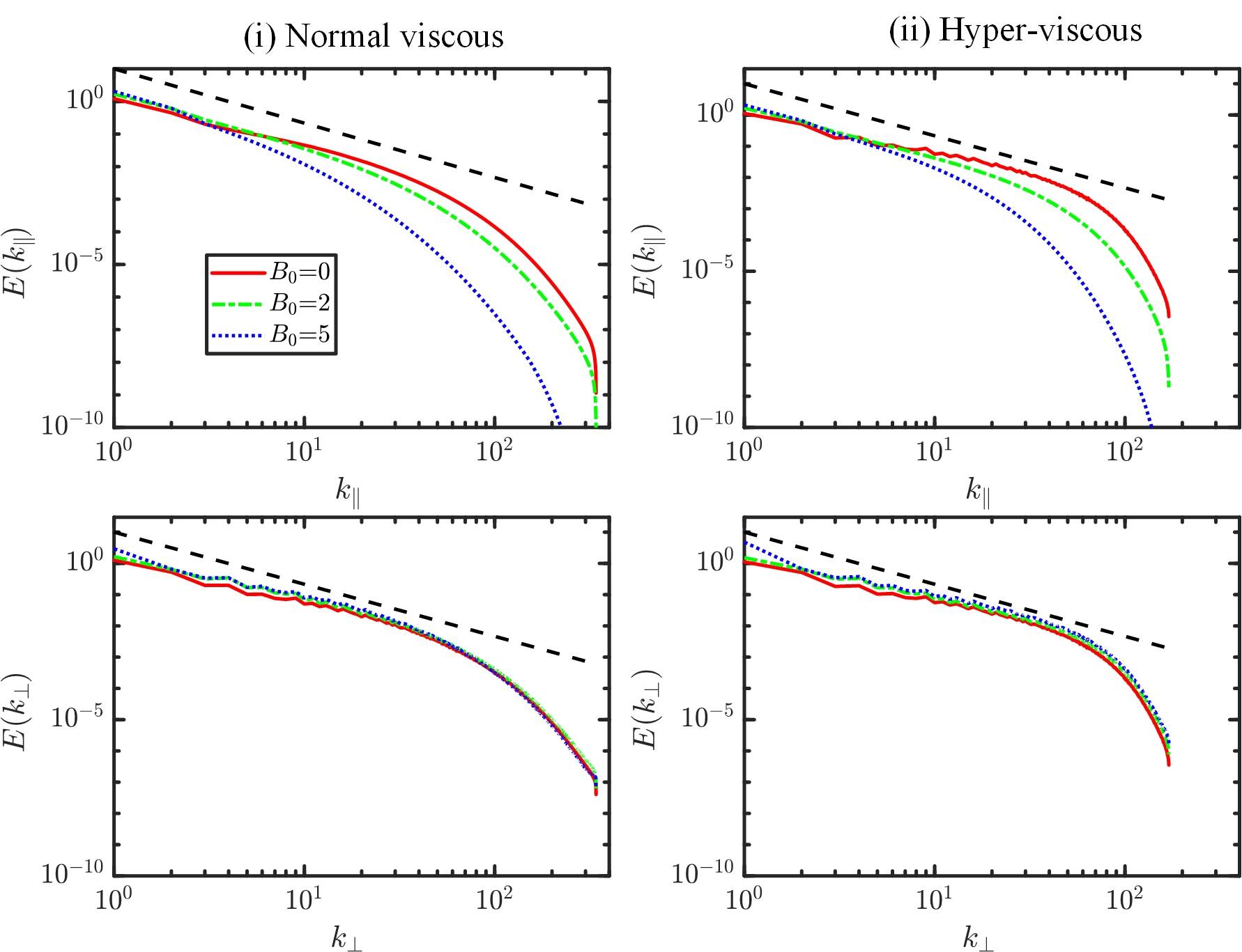
Figure 1: Parallel (top) and perpendicular (bottom) reduced spectra of total energy $E=E_{v}+E_{b}$, $E(k_{\parallel})$ and $E(k_{\perp})$ in normal viscous simulations (left) and hyper-viscous simulations (right). Dashed black lines show $k^{-5/3}$ power law for reference.

Figure 1 shows the reduced spectra of total energy $E=E_{v}+E_{b}$ in the $k_{\parallel}$ and $k_{\perp}$ plane for the normal and hyper-viscous simulations, where $k^{-5/3}$ power law is also shown for reference. The parallel and perpendicular spectra are defined as $E(k_{\parallel})=\int E(k_{\perp},k_{\parallel})dk_{\perp}$ and $E(k_{\perp})=\int E(k_{\perp},k_{\parallel})dk_{\parallel}$, respectively. It is clear that the parallel spectrum is suppressed and the perpendicular spectral transfer is stronger than the parallel transfer with increasing $B_{0}$. This reflects the decreasing of the dissipation rate with the increasing of $B_{0}$ as listed in Table 1. One may observe that higher energy resides in the first $\sim$3 wave modes at larger $B_{0}$ as reported in Ref. (Alexakis et al., 2007b). The inertial range is roughly viewed as the range of scales over which the spectrum fits well with the $k^{-5/3}$ power law. As expected, the simulations with hyperviscosity realize an elongated inertial range.

3 Direction-averaged third-order law

This section describes three types of averaging relevant to the third-order law. Starting from the von Kármán-Howarth (vKH) equation (De Karman & Howarth, 1938; Monin & Yaglom, 1975; Frish, 1995), a general form of the third-order law will be derived. Considering that the present study relates to the effects of an externally supported mean magnetic field, the three types of averaging applied to the general form will be discussed under different assumptions regarding anisotropy.

The vKH equation is typically composed of the time-rate-of-change of energy, energy transfer across scales, and energy dissipation terms, which respectively dominate at energy injection, inertial and dissipation scales. These contributions are evident in the vKH equation itself,

$$\frac{\partial}{\partial t}\langle(\delta\boldsymbol{z}^{\pm})^{2}\rangle=-\nabla_{l}\cdot\langle\delta\boldsymbol{z}^{\mp}|\delta\boldsymbol{z}^{\pm}|^{2}\rangle+2\nu\nabla^{2}_{l}\langle(\delta\boldsymbol{z}^{\pm})^{2}\rangle-4\varepsilon^{\pm}.$$ (6)

Here $\nabla_{l}$ denotes derivatives with respect to the lag vector $\boldsymbol{l}$; $\boldsymbol{Y}^{\pm}=\langle\delta\boldsymbol{z}^{\mp}|\delta\boldsymbol{z}^{\pm}|^{2}\rangle$ is the third-order structure function, also called as (Yaglom) energy-flux vector with the Elsässer variable ($\boldsymbol{z}^{\pm}=\boldsymbol{u}\pm\boldsymbol{b}$) increment being defined as $\delta\boldsymbol{z}^{\pm}(\boldsymbol{x},\boldsymbol{l})=\boldsymbol{z}^{\pm}(\boldsymbol{x}+\boldsymbol{l})-\boldsymbol{z}^{\pm}(\boldsymbol{x})$. $\varepsilon^{\pm}=\nu_{h}\sum\limits_{\boldsymbol{k}}k^{2h}\langle|\hat{\boldsymbol{z}}^{\pm}(\boldsymbol{k},t)|^{2}\rangle$ represent the mean dissipation rates of Elsässer energies.

In the inertial range with negligible contribution from non-stationary and dissipative terms in Eq. (6), the cross-scale energy transfer is expressed as

$$\nabla_{l}\cdot\boldsymbol{Y}^{\pm}=\nabla_{l}\cdot\langle\delta\boldsymbol{z}^{\mp}|\delta\boldsymbol{z}^{\pm}|^{2}\rangle=-4\varepsilon^{\pm},$$ (7)

Note that after ensemble averaging, no dependence of $\boldsymbol{Y}^{\pm}$ on the position $\boldsymbol{x}$ remains, and $\varepsilon^{\pm}$ is independent of both position $\boldsymbol{x}$ and lag $\boldsymbol{l}$.

In anisotropic conditions, as in the present study with imposed external mean magnetic field, Eq. (7) can be reformed by taking a volume integral in a sphere of radius $l$ as follows:

$$\iiint_{|\boldsymbol{l}|\leq l}\nabla_{l}\cdot\boldsymbol{Y}^{\pm}dV=\iiint_{|\boldsymbol{l}|\leq l}-4\varepsilon^{\pm}dV.$$ (8)

Using Gauss’s theorem, Eq.(8) can be written as a surface integral

$$\oint_{|\boldsymbol{l}|=l}Y_{l}^{\pm}dS=\iiint_{|\boldsymbol{l}|\leq l}-4\varepsilon^{\pm}dV=-\frac{16\pi}{3}\varepsilon^{\pm}l^{3},$$ (9)

where $Y_{l}^{\pm}=\langle\delta z_{l}^{\mp}|\delta\boldsymbol{z}^{\pm}|^{2}\rangle$ is the projection of the energy-flux vector along $\boldsymbol{l}$; $\delta z_{l}^{\mp}=\delta\boldsymbol{z}^{\mp}\cdot\frac{\boldsymbol{l}}{l}$, and $l$ is the norm of $\boldsymbol{l}$. In spherical coordinates, Eq.(9) can be written as:

$$\frac{1}{4\pi}\int_{0}^{2\pi}\int_{0}^{\pi}Y_{l}^{\pm}\sin\theta d\theta d\phi=-\frac{4}{3}\varepsilon^{\pm}l,$$ (10)

where $\theta$ represents the polar angle and $\phi$ the azimuthal angle. Note that this integral form Eq. (10) is identical to the derivative form Eq. (7), but it is simpler in the sense that accurate determination of the integration only requires information on the spherical surface spanned by the $(\theta,\phi)$ coordinates in the 3D lag space. (See e.g., Taylor et al. (2003); Wang et al. (2022))

The most general form of $Y_{l}^{\pm}$ should be a function of $l$, $\theta$, and $\phi$, i.e., $Y_{l}^{\pm}(l,\theta,\phi)$. However, there is no universal expression of $Y_{l}^{\pm}(\theta,\phi)$ so far, as little information is available on its variation with turbulence parameters. Previous studies have either been limited to the purely isotropic assumption (i.e., $Y_{l}^{\pm}$ is independent of $\theta$ and $\phi$) or treated anisotropic turbulence with azimuthal symmetry(i.e., $Y_{l}^{\pm}$ is independent of $\phi$) as implemented, for example by Stawarz et al. (2009). Under isotropic assumption, Eq.(10) can be reduced to:

$$\frac{1}{4\pi}\;Y_{l,{\rm isotropic}}^{\pm}\int_{0}^{2\pi}\int_{0}^{\pi}\sin\theta d\theta d\phi=Y_{l,{\rm isotropic}}^{\pm}=-\frac{4}{3}\varepsilon^{\pm}l.$$ (11)

To better understand the anisotropic energy transfer in the inertial range, here we provide a systematic study of $Y_{l}^{\pm}$’s dependence on $\theta$ and $\phi$ with different guide field magnitudes. Specifically, three forms of $Y_{l}^{\pm}$ are discussed:

I) The general form of the third-order structure function for every lag vector $\boldsymbol{l}=(l,\theta,\phi)$ in 3D lag space,

$$Y_{l}^{\pm}(\theta,\phi)=\langle\delta z_{l}^{\mp}|\delta\boldsymbol{z}^{\pm}|^{2}\rangle=Y_{l}^{\pm}(\theta_{i},\phi_{j}),$$ (12)

represents a local radial or longitudinal energy transfer, and ‘local’ means at the specific azimuthal and polar angles, while the total radial energy transfer is the sum of the contributions, i.e. Eq.(12), from all azimuthal $\phi$ and polar $\theta$ directions at the same lag. Due to the axisymmetric external mean magnetic field, the range of $\theta$ is $[0^{\circ},90^{\circ}]$. Lag vectors in 37 directions (there is only one direction at $\theta=0^{\circ}$), uniformly spaced in azimuthal and polar angles ($\Delta\theta=15^{\circ}$ and $\Delta\phi=60^{\circ}$), are used to cover the sphere. A 3D Lagrangian interpolation was used to attain the data not located at grid points. Separate estimates are made for each of 37 directions, i.e., $Y_{l}^{\pm}(\theta_{i},\phi_{j})$, $\theta_{i}\in[0^{\circ}:15^{\circ}:90^{\circ}]$ and $\phi_{j}\in[0^{\circ}:60^{\circ}:300^{\circ}]$.

II) The azimuthal averaged form of the third-order structure function,

$$\widetilde{Y_{l}^{\pm}}(\theta)=\frac{1}{2\pi}\int_{0}^{2\pi}Y_{l}^{\pm}(\theta,\phi)d\phi\approx\frac{\sum_{j=1}^{N_{j}}Y_{l}^{\pm}(\theta_{i},\phi_{j})}{N_{j}},$$ (13)

describes the anisotropy of local radial energy transfer, and ‘local’ means at a specific polar angle, while the total transfer rate is the sum of the contributions, i.e. Eq.( 13), from all polar $\theta$ directions at the same lag. $N_{j}$(=6) represents the number of azimuthal angles. Following Eq. (12), separate estimates are made for each of 37 directions, and then averaged over 6 azimuthal directions.

III) The direction-averaged form of the third-order structure function,

$$\overline{Y_{l}^{\pm}}=\frac{1}{4\pi}\int_{0}^{2\pi}\int_{0}^{\pi}Y_{l}^{\pm}\sin\theta d\theta d\phi\approx\frac{\sum_{j=1}^{N_{j}}\sum_{i=1}^{N_{i}}Y_{l}^{\pm}(\theta_{i},\phi_{j})\sin\theta_{i}}{N_{j}\sum_{i=1}^{N_{i}}\sin\theta_{i}},$$ (14)

is rather general since it takes into account all possible anisotropy in both azimuthal and polar directions. $N_{i}$(=7) and $N_{j}$(=6) represent the number of angle $\theta$ and $\phi$. This direction-averaged form of the third-order structure function is derived directly from the vKH equation without the assumption of isotropy and only depends on the lag length $l$. After normalizing $\overline{Y_{l}^{\pm}}$ with the lag $-4/3l$, it can represent an accurate estimation of the cross-scale energy transfer rate (or energy dissipation rate $\varepsilon_{diss}$) and the inertial range.

The aforementioned description of the energy transfer in the three forms of third-order structure functions can provide estimations of the actual energy transfer rate to different degrees. For instance, Eq.(12) has been widely used in the observational measurements with one spacecraft. To clearly show the estimation of the energy transfer rate and the inertial range, the aforementioned three forms of the third-order structure functions, i.e., $Y_{l}^{\pm}$, $\widetilde{Y_{l}^{\pm}}$ and $\overline{Y_{l}^{\pm}}$, will be averaged on their $+$ and $-$ components and normalized with the lag and the actual cascade rate, i.e. $-\frac{4}{3}\varepsilon_{diss}l$, where $\varepsilon_{diss}$ is the total cascade rate, $\varepsilon_{diss}=(\varepsilon^{+}+\varepsilon^{-})/2=\varepsilon_{b}+\varepsilon_{v}$.

4 Results and Discussion

This section will make a comparison between normal viscous and hyper-viscous cases and focus on the angular dependence of third-order structure functions under various strengths of the external magnetic field. In addition, the possible effect of time averaging will be discussed.

4.1 Effects of hyperviscosity and polar angle dependence

In anisotropic MHD turbulence with a mean magnetic field, the energy transfer is often deemed to be isotropic in the plane perpendicular to $B_{0}$ direction, that is, $Y_{l}^{\pm}$ is $\phi$ independent. So as a first analysis, we integrate $Y_{l}^{\pm}$ over $\phi$ and time average over long statistically stationary periods and attain a normalized third-order structure function as: $-3(\widetilde{Y_{l}^{+}}+\widetilde{Y_{l}^{-}})/(4\varepsilon_{diss}l)$.

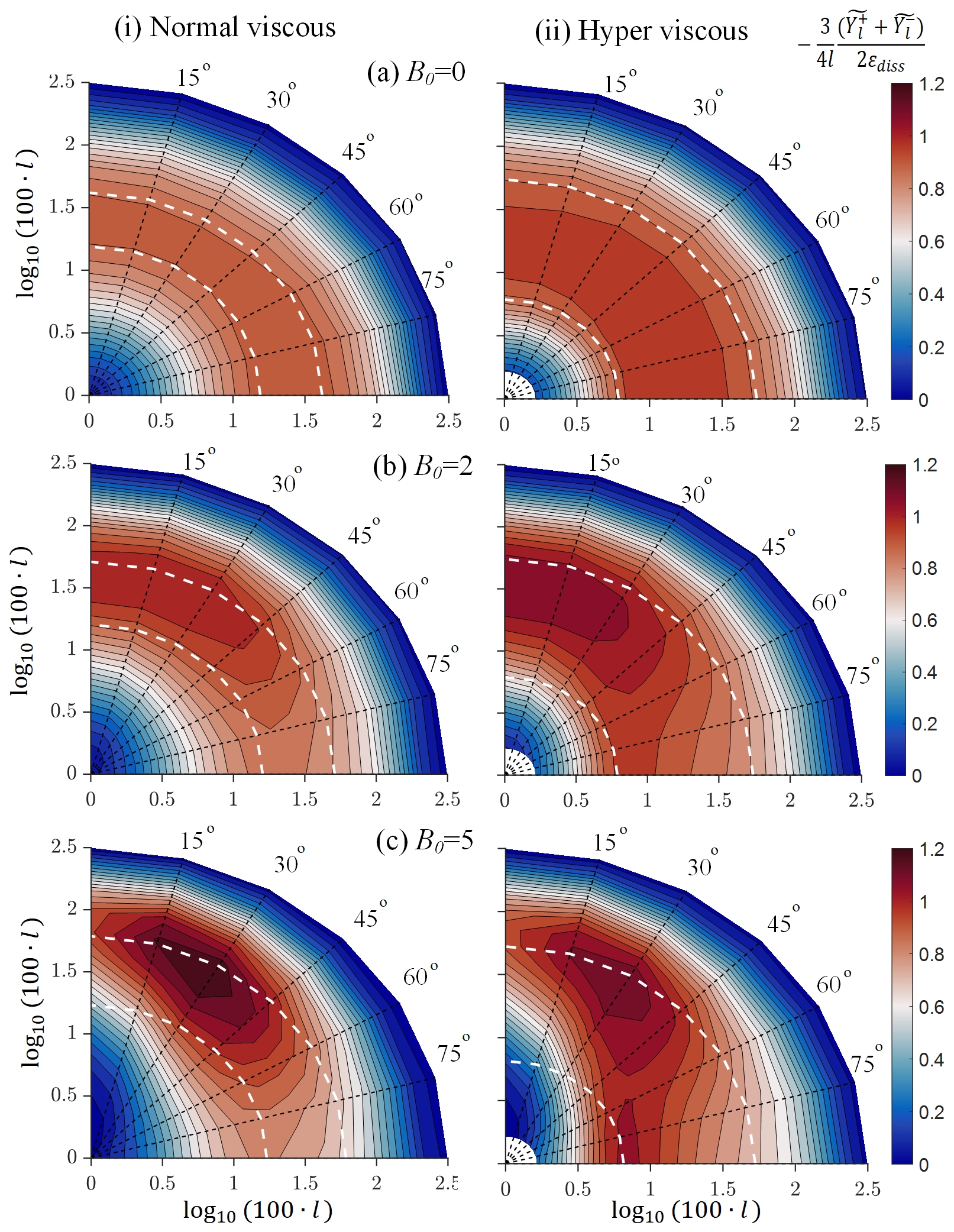
Figure 2: Comparison of normalized third-order structure functions, i.e. $-3(\widetilde{Y_{l}^{+}}+\widetilde{Y_{l}^{-}})/(4\varepsilon_{diss}l)$ between (i) simulations with normal viscosity and (ii) simulations with hyperviscosity with polar angles ranging $\theta=$ [0^∘:15^∘:90^∘]. $\theta=0^{\circ}$ represents parallel direction relative to $\boldsymbol{B}_{0}$, and $\theta=90^{\circ}$ represents perpendicular direction relative to $\boldsymbol{B}_{0}$. The white dashed lines represent the inertial range, identified with the direction-averaged form of third-order law, where the $-3(\overline{Y_{l}^{+}}+\overline{Y_{l}^{-}})/(4\varepsilon_{diss}l)$ is beyond a threshold, say 0.9. All contours are integrated over $\phi$ and time. For the visualisation of the inertial range, the $x$-axis is transformed into the $\log_{10}{(100l)}$.

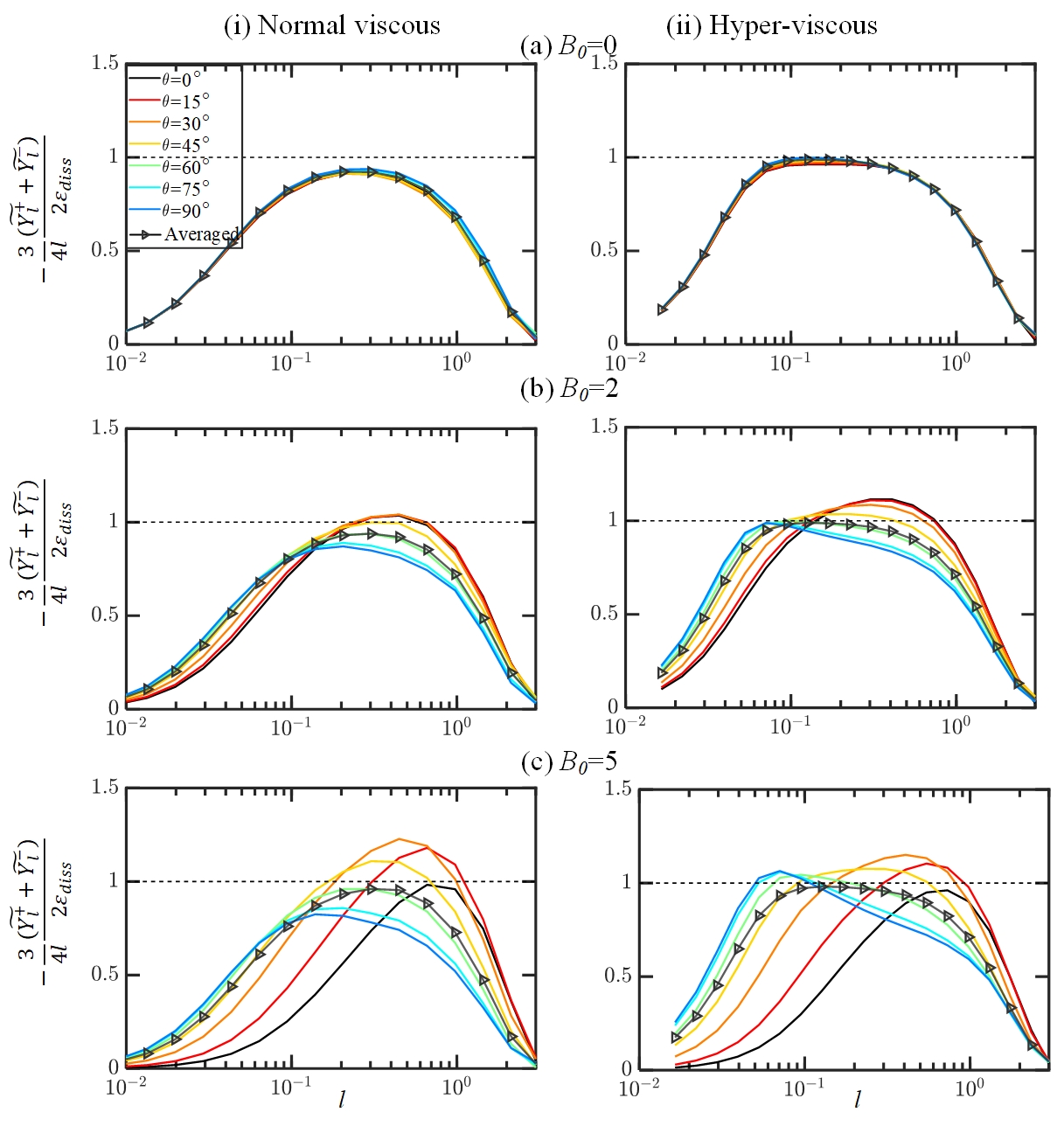
Figure 3: Comparison of normalized third-order structure functions, i.e. $-3(\widetilde{Y_{l}^{+}}+\widetilde{Y_{l}^{-}})/(4\varepsilon_{diss}l)$, at $B_{0}=0,2,5$ between (i) normal viscous and (ii) hyper-viscous simulations with $\theta=$ [0^∘:15^∘:90^∘], and the solid line with triangles represents the direction-averaged profile, i.e. $-3(\overline{Y_{l}^{+}}+\overline{Y_{l}^{-}})/(4\varepsilon_{diss}l)$. All curves are averaged over $\phi$ and time. For nonzero $B_{0}$ the estimated transfer rate peaks at large scales for parallel angles, and at progressively smaller scales for perpendicular angles.

Figure 2 shows contour of the averaged and normalized third-order structure functions for both normal viscous and hyper-viscous cases with various values of $B_{0}$. The inertial range are identified with the direction-averaged form of third-order law, where the $-3(\overline{Y_{l}^{+}}+\overline{Y_{l}^{-}})/(4\varepsilon_{diss}l)$ is beyond a threshold, say 0.9, and marked with the white dashed lines. A straightforward observation is that the isotropic cases at $B_{0}=$ 0 present a distribution of the normalized structure functions that is essentially independent of polar angle $\theta$. Unlike this isotropic case ($B_{0}$=0), the dark contour lines for $B_{0}=2$ and 5 do not distribute symmetrically. More specifically, the contour lines at small $l$ (dark blue regions close to origins) are elongated along the parallel direction $\theta=0^{\circ}$, which can be interpreted as the anisotropy introduced by the mean magnetic field. The contour lines at large $l$ (dark blue outer regions) approach a more circular conformation. This is not in conflict with the frequently observed picture of anisotropy in decaying MHD turbulence, as the present system is driven isotropically at large scales. The inertial range exists in the transition region between small and large scales as marked with the white dashed lines. For nonzero $B_{0}$ cases, the peak value of the normalized third-order structure function at larger $\theta$ occurs at smaller scales, which is consistent with the results in Refs. (Verdini et al., 2015; Wang et al., 2022). The maximum radial transfer rate shifts away from $B_{0}$ direction at larger $B_{0}$, with the corresponding $\theta$ of the maxima for $B_{0}=$ 2 and 5 is $\theta=0^{\circ}$ and $\theta=30^{\circ}$, respectively, which is more clear in Figure 3.

We can see the clear difference between normal and hyper-viscous cases in Figure 3, where the normalized third-order structure functions at $\theta\in[0^{\circ}:15^{\circ}:90^{\circ}]$ are shown. Also shown is the normalized and direction-averaged third-order structure function, i.e. $-3(\overline{Y_{l}^{+}}+\overline{Y_{l}^{-}})/(4\varepsilon_{diss}l)$. Even though the normalized third-order structure functions exhibit evident dependence on $\theta$, the direction-averaged third-order law attains an accurate cascade rate with less than 5$\%$ error for all cases. The plateau of the direction-averaged form in the Figure 3 gives a rough idea of the inertial range, which indicates that $l\in[0.15,0.43]$ and $l\in[0.06,0.55]$ at $B_{0}=0$ can be roughly identified as the inertial range for the normal and hyper-viscous cases, respectively. This elongated inertial range is also consistent with the estimates of the inertial range in Figure 1, where $k=\pi/l$. Therefore, as expected, hyperviscosity enables a wider inertial range than normal viscosity and the longer inertial range is beneficial to examine the third-order law.

The hyper-viscous cases show a similar polar angle dependence to the normal viscous cases at low $B_{0}$ (i.e., weak anisotropy). At $B_{0}=0$, the individual $\theta$ profiles in Figure 3 overlap with the direction-averaged profile, indicating the validity of the 1D isotropic third-order law. As $B_{0}$ increases, they deviate from the direction-averaged profile. In particular, when $B_{0}$ is large enough (e.g. the bottom row in Figure 3 with $B_{0}=5$), the third-order structure functions for the hyper-viscous cases exhibit distinct peak values from the normal viscous cases. For the normal viscous case, the third-order law tends to underestimate the cascade rate for $\theta>45^{\circ}$, while overestimate the cascade rate for $\theta<$45^∘. As such, the maximum value of the estimated cascade rate locates at $\theta=30^{\circ}$, also shown in Figure 2. In contrast, for the hyper-viscous case, the third-order law at $\theta\sim 90^{\circ}$ overestimates the cascade rate and the contour map in Figure 2 exhibits two local maxima at $\theta=30^{\circ}$ and $\theta=90^{\circ}$. The maximum at $\theta=90^{\circ}$ could be attributed to the dissipation concentrated at smaller scales due to hyperviscosity. As we can see, the energy transfer changes gradually with angles and the most efficient transfer may not necessarily occur in the strictly perpendicular direction.

4.2 Azimuthal angle dependence

In this subsection, the hyper-viscous cases will be used to demonstrate the azimuthal dependence of the third-order structure function. The left column of Figure 4 shows the normalized third-order structure function at different $\theta$ and $\phi$. For the each series of the line with the same color, the $\theta$ is fixed and $\phi$ is varied. It can be seen that the variability of third-order structure functions in the azimuthal and polar angles increases with the increase of $B_{0}$, indicated by the more scattered distribution of the profiles at higher $B_{0}$. Specifically, at $B_{0}=0$, these individual lines almost collapse, indicating the isotropic features in both the polar and azimuthal directions. At $B_{0}=2$, the peak values of these lines are almost beyond unity. At $B_{0}=5$, the peaks vary beyond and below the unity. To further quantify these departures from the actual cascade rates in Table 1, the right column of Figure 4 is plotted by using the peak of each profile, representing the estimated cascade rate. The distribution of these estimates, as marked with the dark circles, is more scatter at a larger $B_{0}$. At $B_{0}=2,5$, the maximum estimated cascade rate can depart from the actual value by 10$\%$ and $25\%$ and both at $\theta=45^{\circ}$. We expect this departure to be even greater at larger $B_{0}$. From the red line in the right column of Figure 4, after doing the azimuthal average, the maximum departures from unity reduces to 3$\%$ and 15$\%$ at $B_{0}=2,5$, respectively.

Theoretically, given that the number of frames is enough to do the average, the structure function should be independent of the azimuthal angles, or the energy transfer is isotropic in the perpendicular plane. However, in some contexts, the sampling dataset is limited to finite snapshots as in DNS or directions as in observations, as such the dependence may exist on the azimuthal directions. An adequate coverage of azimuthal angles is required to obtain an accurate estimation of cascade rates. To further check the mutual impact of the time and angle averages, the effects of the sampling time will be discussed in the next subsection.

Figure 4: (a) Normalized third-order structure functions, i.e. $-3({Y_{l}^{+}}+Y_{l}^{-})/(4\varepsilon_{diss}l)$, for (i) $B_{0}=0$, (ii) $B_{0}=2$ and (iii) $B_{0}=5$ hyper-viscous cases at different $\theta$ and $\phi$. Each series of colors represents a fixed $\theta$ and varied $\phi$. (b) estimated cascade rates from column (a) by extracting the peaks of each curves and then normalized with the total dissipation rate, $\varepsilon_{diss}$. The solid line with circles represents the averaged profile on the azimuthal direction. All curves are time averaged.

4.3 Effects of time averaging

In this subsection, the hyper-viscous cases will be used to demonstrate the effect of time averaging. At least two aspects of the time averaging are of central importance, one being the time interval (or sampling frequency) $\Delta T$, and the other being the length of periods $T$. We can expect that in our driven cases, the smaller $\Delta T$ and the longer $T$, the more reliable statistics. The time interval $\Delta T$ ($\Delta T<T_{e}$, where $T_{e}$ is the large-eddy turnover time) does not show significant impacts on the third-order structure function in our cases (Figures are not shown here). Therefore, in the following analysis, we fix $\Delta T=0.5T_{e}$ and focus on the effect of the length of periods $T$. These periods are within the statistically stationary periods listed in Table 1.

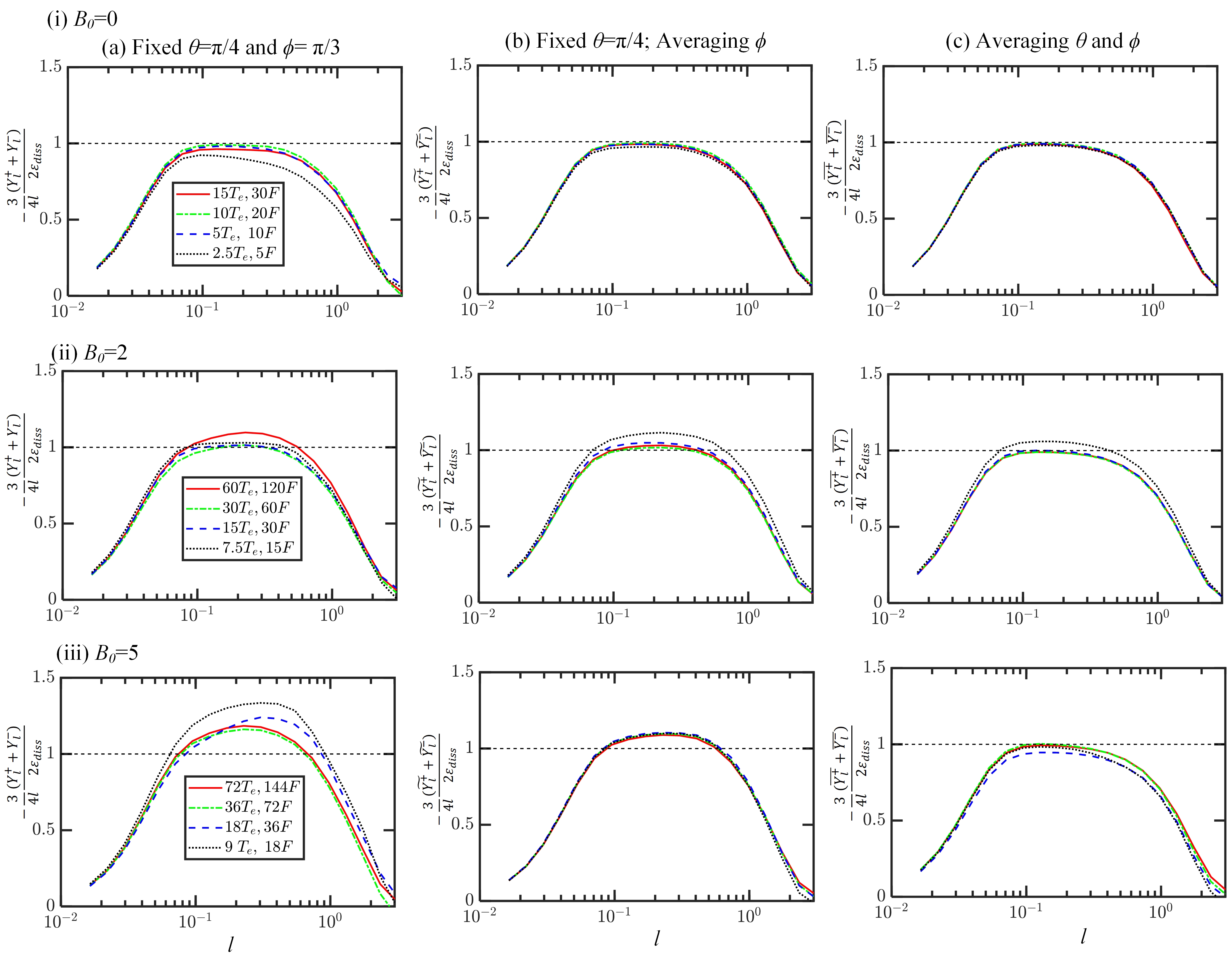
Figure 5: Effects of the number of time frames on the calculation of the normalized third-order structure functions at (i) $B_{0}=0$, (ii) $B_{0}=2$ and (iii) $B_{0}=5$ for the hyper-viscous cases. Left column (a): fixed $\theta=\pi/4;\phi=\pi/3$. Middle column (b): fixed $\theta=\pi/4$ and azimuthal-averaged profiles. Right column (c): direction-averaged profiles. $T_{e}$ denotes the large-eddy turnover time at $B_{0}=0$, and $F$ represents the number of frames used in the time average.

Figure 5 shows the effect of the length of periods (or the number of time frames, $F$) on the third-order structure function. The third-order law at fixed $\theta$ and $\phi$ as Eq. (12), at fixed $\theta$ but $\phi$ averaged as Eq. (13) and both $\theta$ and $\phi$ averaged as Eq. (14) is shown in left, middle and right columns, respectively. Three key observations can be found:

i) the direction-averaged profiles require less time frames ($F$) to converge than the profiles with fixed $\theta$ and $\phi$. For instance, at $B_{0}=$ 5 the direction-averaged profiles converge with 36 time snapshots, while the profiles with fixed $\theta$ and $\phi$ are not converged until 72 time frames are employed.

ii) a smaller $B_{0}$ requires a lesser number of frames to converge. The required number of time frames for $B_{0}=$ 0 and $B_{0}=$ 5 to converge are about 10 and 70, respectively, without the directional average (column (a) in Figure 5). These times are reduced to about 5 and 30, respectively, with directional averaging (see column (c) in Figure 5.)

iii) sufficient time averaging cannot make up for the lack of angle coverage, indicated by the different peak values of non-direction-averaged and direction-averaged profiles in the anisotropic cases. Also, by comparing the three columns, the angle averaging makes the plateaus of these plots closer to the actual dissipation rate. For instance, at $B_{0}=5$, the converged profiles without angular averaging, with only azimuthal averaging and with both azimuthal and polar averaging attain peak values of 1.19, 1.09 and 0.98, respectively. This indicates that, compared with the time averaging, the angle averaging is a more effective way to make the calculation of the structure function converge.

5 Conclusions

3D simulations of incompressible MHD turbulence with normal and hyperviscosity were conducted with different externally supported (mean) uniform magnetic fields to systematically study the effect of external mean magnetic fields on the cross-scale energy transfer and the third-order law. Three different forms of third-order structure functions were calculated with or without the averaging the azimuthal and polar angles. The results show that, compared with the normal viscous cases, the hyperviscosity elongates and separates the inertial range from the dissipation range, thus helping the examination of the above-mentioned forms of third-order law.

The direction-averaged third-order law can predict the energy cascade rates and inertial range accurately, even at very high $B_{0}$ (see background on this in Taylor et al. (2003) and Wang et al. (2022)). However, the third-order law is highly dependent on the polar angle in anisotropic MHD turbulence. The azimuthal angle dependence we find here is counterintuitive, in that the statistics are usually deemed to be isotropic in the perpendicular plane to $B_{0}$. This azimuthal angle dependence was further confirmed with an examination of the number of averaging time frames. More time frames are required to make the calculation of the third-order structure function converge in the anisotropic condition, especially at high $B_{0}$. However, even using the enough time frames, the structure function profiles with and without the azimuthal average are still different. We conclude that the time averaging cannot make up for a lack of angle-averaging, especially at large values of mean magnetic field $B_{0}$.

An interesting finding, also seen in earlier studies Verdini et al. (2015); Wang et al. (2022), is that identified peaks or plateaus of the estimated transfer rate occur at different scales for different angles to the mean magnetic field. Accordingly, this also means that the inertial range will be assigned to different ranges of scales. Our use of hyperviscosity shows that this method produces an extended plateau, facilitating analysis of inertial range properties. Future studies may find a rationale for understanding how these different ranges come into being, as the balance of local transfer rate competes with dissipation at different angles. Such analyses may require examination of the vector character of the Yaglom energy flux, a subject that we have not engaged in here. It should be noted however that there are some studies that have begun such analyses, typically by making assumptions regarding the symmetry of the transfer. Examples include the 2D (perpendicular) + 1D (parallel) model employed by MacBride & Smith (2008); Stawarz et al. (2009, 2010). Such models may require further refinement since at least some prior models enforce the questionable assumption that the transfers of energy in parallel and perpendicular directions are independent.

Funding.   We acknowledge the support from NSFC (Grant Nos. 12225204, and 11902138); Department of Science and Technology of Guangdong Province (Grant Nos. 2019B21203001 and 2020B1212030001); the Shenzhen Science and Technology Program (Grant No. KQTD20180411143441009). Y.Y. and W.H.M. are supported by NSF grant AGS02108834 and by NASA under the IMAP project at Princeton (subcontract 0000317 to Delaware). W.H.M.is also supported as a Co-Investigator on the Helioswarm project. The assistance of resources and services from the Center for Computational Science and Engineering of Southern University of Science and Technology is also acknowledged.

Declaration of interests. The authors report no conflict of interest.

References

- Alexakis et al. (2007a) Alexakis, A., Bigot, B., Politano, H. & Galtier, S. 2007a Anisotropic fluxes and nonlocal interactions in magnetohydrodynamic turbulence. Phys. Rev. E 76, 056313.
- Alexakis et al. (2007b) Alexakis, A, Bigot, B, Politano, Hélène & Galtier, S 2007b Anisotropic fluxes and nonlocal interactions in magnetohydrodynamic turbulence. Physical Review E 76 (5), 056313.
- Andrés et al. (2019) Andrés, N., Sahraoui, F., Galtier, S., Hadid, L. Z., Ferrand, R. & Huang, S. Y. 2019 Energy cascade rate measured in a collisionless space plasma with mms data and compressible hall magnetohydrodynamic turbulence theory. Phys. Rev. Lett. 123, 245101.
- Antonia et al. (1997) Antonia, RA, Ould-Rouis, M, Anselmet, F & Zhu, Y 1997 Analogy between predictions of kolmogorov and yaglom. Journal of Fluid Mechanics 332, 395–409.
- Bandyopadhyay et al. (2020) Bandyopadhyay, Riddhi, Sorriso-Valvo, Luca, Chasapis, Alexand ros, Hellinger, Petr, Matthaeus, William H., Verdini, Andrea, Landi, Simone, Franci, Luca, Matteini, Lorenzo, Giles, Barbara L., Gershman, Daniel J., Moore, Thomas E., Pollock, Craig J., Russell, Christopher T., Strangeway, Robert J., Torbert, Roy B. & Burch, James L. 2020 In Situ Observation of Hall Magnetohydrodynamic Cascade in Space Plasma. Phys Rev. Lett. 124 (22), 225101, arXiv: 1907.06802.
- Banerjee et al. (2016) Banerjee, S., Hadid, L. Z., Sahraoui, F. & Galtier, S. 2016 Scaling of compressible magnetohydrodynamic turbulence in the fast solar wind. Astrophys. J. Lett. 829, L27.
- Beresnyak & Lazarian (2009) Beresnyak, Andrey & Lazarian, Alex 2009 Comparison of spectral slopes of magnetohydrodynamic and hydrodynamic turbulence and measurements of alignment effects. The Astrophysical Journal 702 (2), 1190.
- Biskamp (2003) Biskamp, Dieter 2003 Magnetohydrodynamic turbulence. Cambridge University Press.
- Biskamp & Müller (2000) Biskamp, Dieter & Müller, Wolf-Christian 2000 Scaling properties of three-dimensional isotropic magnetohydrodynamic turbulence. Physics of Plasmas 7 (12), 4889–4900.
- Bruno & Carbone (2013) Bruno, Roberto & Carbone, Vincenzo 2013 The Solar Wind as a Turbulence Laboratory. Living Reviews in Solar Physics 10 (1), 2.
- Carbone et al. (2009) Carbone, V., Marino, R., Sorriso-Valvo, L., Noullez, A. & Bruno, R. 2009 Scaling laws of turbulence and heating of fast solar wind: the role of density fluctuations. Phys. Rev. Lett. 103, 061102.
- Coleman (1968) Coleman, P. J. 1968 Turbulence, viscosity, and dissipation in the solar wind plasma. Astrophys. J. 153, 371–388.
- De Karman & Howarth (1938) De Karman, Theodore & Howarth, Leslie 1938 On the statistical theory of isotropic turbulence. Proceedings of the Royal Society of London. Series A-Mathematical and Physical Sciences 164 (917), 192–215.
- Ferrand et al. (2019) Ferrand, Renaud, Galtier, Sébastien, Sahraoui, Fouad, Meyrand, Romain, Andrés, Nahuel & Banerjee, Supratik 2019 On exact laws in incompressible hall magnetohydrodynamic turbulence. The Astrophysical Journal 881 (1), 50.
- Ferrand et al. (2022) Ferrand, R, Sahraoui, F, Galtier, S, Andrés, N, Mininni, P & Dmitruk, P 2022 An in-depth numerical study of exact laws for compressible hall magnetohydrodynamic turbulence. arXiv preprint arXiv:2201.10819 .
- Frisch (1995) Frisch, U. 1995 Turbulence. The legacy of A. N. Kolmogorov..
- Frish (1995) Frish, U 1995 Turbulence: The legacy of an kolmogorov cambridge. New York .
- Galtier (2009) Galtier, S 2009 Exact vectorial law for axisymmetric magnetohydrodynamics turbulence. The Astrophysical Journal 704 (2), 1371.
- Gogoberidze et al. (2013) Gogoberidze, G, Perri, S & Carbone, V 2013 The yaglom law in the expanding solar wind. The Astrophysical Journal 769 (2), 111.
- Hadid et al. (2017) Hadid, LZ, Sahraoui, F & Galtier, S 2017 Energy cascade rate in compressible fast and slow solar wind turbulence. The Astrophysical Journal 838 (1), 9.
- Hellinger et al. (2013) Hellinger, Petr, Trávníček, Pavel M, Štverák, Štěpán, Matteini, Lorenzo & Velli, Marco 2013 Proton thermal energetics in the solar wind: Helios reloaded. Journal of Geophysical Research: Space Physics 118 (4), 1351–1365.
- Hellinger et al. (2018) Hellinger, Petr, Verdini, Andrea, Landi, Simone, Franci, Luca & Matteini, Lorenzo 2018 von kármán–howarth equation for hall magnetohydrodynamics: Hybrid simulations. The Astrophysical Journal Letters 857 (2), L19.
- Horbury et al. (2008) Horbury, T. S., Forman, M. & Oughton, S. 2008 Anisotropic scaling of magnetohydrodynamic turbulence. Phys. Rev. Lett. 101.
- Hossain et al. (1995) Hossain, Murshed, Gray, Perry C, Pontius Jr, Duane H, Matthaeus, William H & Oughton, Sean 1995 Phenomenology for the decay of energy-containing eddies in homogeneous mhd turbulence. Physics of Fluids 7 (11), 2886–2904.
- Jokipii & Hollweg (1970) Jokipii, J. R. & Hollweg, J. V. 1970 Interplanetary Scintillations and the Structure of Solar-Wind Fluctuations. apj 160, 745.
- de Kármán & Howarth (1938) de Kármán, T. & Howarth, L. 1938 On the statistical theory of isotropic turbulence. Proc. Roy. Soc. London Ser. A 164, 192–215.
- Kolmogorov (1941a) Kolmogorov, AN 1941a Dissipation of energy in locally isotropic turbulence in an incompressible viscous liquid. In Dokl. Akad. Nauk SSSR, , vol. 30, pp. 299–303.
- Kolmogorov (1941b) Kolmogorov, A. N. 1941b Local structure of turbulence in an incompressible viscous fluid at very high Reynolds numbers. Dokl. Akad. Nauk SSSR 30, 301–305, [Reprinted in Proc. R. Soc. London, Ser. A 434, 9–13 (1991)].
- Kolmogorov (1941c) Kolmogorov, A. N. 1941c On degeneration of isotropic turbulence in an incompressible viscous liquid. C.R. Acad. Sci. U.R.S.S. 31, 538–540.
- Kraichnan (1971) Kraichnan, R. H. 1971 Inertial-range transfer in two- and three-dimensional turbulence. J. Fluid Mech. 47, 525.
- Kritsuk et al. (2009) Kritsuk, A. G., Ustyugov, S. D., Norman, M. K. & Padoan, P. 2009 Simulating supersonic turbulence in magnetized molecular clouds. J. Phys. Conf. Ser. 180, 012020.
- MacBride & Smith (2008) MacBride, Benjamin T. & Smith, Charles W. 2008 The turbulent cascade at 1 AU: energy transfer and the third-order scaling for MHD. Astrophys. J. 679, 1644–1660.
- Matthaeus et al. (2019) Matthaeus, W. H., Bandyopadhyay, R., Brown, M. R., Borovsky, J., Carbone, V., Caprioli, D., Chasapis, A., Chhiber, R., Dasso, S., Dmitruk, P., Del Zanna, L., Dmitruk, P. A., Franci, Luca, Gary, S. P., Goldstein, M. L., Gomez, D., Greco, A., Horbury, T. S., Ji, Hantao, Kasper, J. C., Klein, K. G., Landi, S., Li, Hui, Malara, F., Maruca, B. A., Mininni, P., Oughton, Sean, Papini, E., Parashar, T. N., Petrosyan, Arakel, Pouquet, Annick, Retino, A., Roberts, Owen, Ruffolo, David, Servidio, Sergio, Spence, Harlan, Smith, C. W., Stawarz, J. E., TenBarge, Jason, Vasquez1, B. J., Vaivads, Andris, Valentini, F., Velli, Marco, Verdini, A., Verscharen, Daniel, Whittlesey, Phyllis, Wicks, Robert, Bruno, R. & Zimbardo, G. 2019 [plasma 2020 decadal] the essential role of multi-point measurements in turbulence investigations: the solar wind beyond single scale and beyond the taylor hypothesis.
- Matthaeus et al. (1996) Matthaeus, W. H., Ghosh, S., Oughton, S. & Roberts, D. A. 1996 Anisotropic three-dimensional MHD turbulence. J. Geophys. Res. 101, 7619–7629.
- Matthaeus & Goldstein (1982) Matthaeus, W. H. & Goldstein, M. L. 1982 Measurement of the rugged invariants of magnetohydrodynamic turbulence in the solar wind. J. Geophys. Res. 87, 6011–6028.
- Monin & Yaglom (1975) Monin, AS & Yaglom, AM 1975 Statistical fluid mechanics: Mechanics of turbulence, vol. 2, 874 pp.
- Nie & Tanveer (1999) Nie, Qing & Tanveer, S 1999 A note on third–order structure functions in turbulence. Proceedings of the Royal Society of London. Series A: Mathematical, Physical and Engineering Sciences 455 (1985), 1615–1635.
- Osman et al. (2011a) Osman, K. T., Matthaeus, W. H., Greco, A. & Servidio, S. 2011a Evidence for inhomogeneous heating in the solar wind. Astrophys. J. Lett. 727, L11.
- Osman et al. (2011b) Osman, K. T., Wan, M., Matthaeus, W. H., Weygand, J. M. & Dasso, S. 2011b Anisotropic third-moment estimates of the energy cascade in solar wind turbulence using multispacecraft data. Phys. Rev. Lett. 107, 165001.
- Oughton et al. (2015) Oughton, S., Matthaeus, W. H., Wan, M. & Osman, K. T. 2015 Anisotropy in solar wind plasma turbulence. Phil Trans. Roy. Soc. A 373.
- Parker (1979) Parker, E. N. 1979 Cosmical Magnetic Fields: Their Origin and Activity. Oxford, UK: Oxford Univeristy Press.
- Podesta (2008) Podesta, JJ 2008 Laws for third-order moments in homogeneous anisotropic incompressible magnetohydrodynamic turbulence. Journal of Fluid Mechanics 609, 171–194.
- Podesta et al. (2007) Podesta, JJ, Forman, MA & Smith, CW 2007 Anisotropic form of third-order moments and relationship to the cascade rate in axisymmetric magnetohydrodynamic turbulence. Physics of Plasmas 14 (9), 092305.
- Politano & Pouquet (1998) Politano, H & Pouquet, A 1998 von kármán–howarth equation for magnetohydrodynamics and its consequences on third-order longitudinal structure and correlation functions. Physical Review E 57 (1), R21.
- Shebalin et al. (1983) Shebalin, John V, Matthaeus, William H & Montgomery, David 1983 Anisotropy in mhd turbulence due to a mean magnetic field. Journal of Plasma Physics 29 (3), 525–547.
- Spence (2019) Spence, H. E. 2019 HelioSwarm: Unlocking the Multiscale Mysteries of Weakly-Collisional Magnetized Plasma Turbulence and Ion Heating. In AGU Fall Meeting Abstracts, , vol. 2019, pp. SH11B–04.
- Spyksma et al. (2012) Spyksma, Kyle, Magcalas, Moriah & Campbell, Natalie 2012 Quantifying effects of hyperviscosity on isotropic turbulence. Physics of Fluids 24 (12), 125102.
- Stawarz et al. (2009) Stawarz, Joshua E., Smith, Charles W., Vasquez, Bernard J., Forman, Miriam A. & MacBride, Benjamin T. 2009 The turbulent cascade and proton heating in the solar wind at 1 AU. Astrophys. J. 697, 1119–1127.
- Stawarz et al. (2010) Stawarz, J. E., Smith, C. W., Vasquez, B. J., Forman, M. A. & MacBride, B. T. 2010 The turbulent cascade for high cross-helicity states at 1 au. Astrophys. J. 713, 920–934.
- Stawarz et al. (2011) Stawarz, Joshua E, Vasquez, Bernard J, Smith, Charles W, Forman, Miriam A & Klewicki, Joseph 2011 Third moments and the role of anisotropy from velocity shear in the solar wind. The Astrophysical Journal 736 (1), 44.
- Taylor (1938) Taylor, G. I. 1938 The spectrum of turbulence. Proc. Roy. Soc. Lond. A 164, 476–490.
- Taylor et al. (2003) Taylor, M. A., Kurien, S. & Eyink, G. L. 2003 Recovering isotropic statistics in turbulence simulations: The Kolmogorov 4/5th law. Phys. Rev. E 68, 026310.
- Tu & Marsch (1995) Tu, C.-Y. & Marsch, E. 1995 MHD structures, waves and turbulence in the solar wind. Space Sci. Rev. 73, 1–210.
- Verdini et al. (2015) Verdini, Andrea, Grappin, Roland, Hellinger, Petr, Landi, Simone & Müller, Wolf Christian 2015 Anisotropy of third-order structure functions in mhd turbulence. The Astrophysical Journal 804 (2), 119.
- Verdini et al. (2015) Verdini, Andrea, Grappin, Roland, Hellinger, Petr, Landi, Simone & Müller, Wolf Christian 2015 Anisotropy of Third-order Structure Functions in MHD Turbulence. Astrophys. J. 804 (2), 119, arXiv: 1502.04705.
- Wan et al. (2009) Wan, Minping, Servidio, Sergio, Oughton, Sean & Matthaeus, William H 2009 The third-order law for increments in magnetohydrodynamic turbulence with constant shear. Physics of plasmas 16 (9), 090703.
- Wan et al. (2010) Wan, Minping, Servidio, Sergio, Oughton, Sean & Matthaeus, William H 2010 The third-order law for magnetohydrodynamic turbulence with shear: Numerical investigation. Physics of Plasmas 17 (5), 052307.
- Wang et al. (2022) Wang, Yanwen, Chhiber, Rohit, Adhikari, Subash, Yang, Yan, Bandyopadhyay, Riddhi, Shay, Michael A, Oughton, Sean, Matthaeus, William H & Cuesta, Manuel E 2022 Strategies for determining the cascade rate in mhd turbulence: isotropy, anisotropy, and spacecraft sampling. The Astrophysical Journal 937 (2), 76.
- Yang et al. (2021) Yang, Yan, Linkmann, Moritz, Biferale, Luca & Wan, Minping 2021 Effects of forcing mechanisms on the multiscale properties of magnetohydrodynamics. The Astrophysical Journal 909 (2), 175.
- Yang et al. (2017) Yang, Y., Matthaeus, W. H., Shi, Y., Wan, M. & Chen, S. 2017 Compressibility effect on coherent structures, energy transfer and scaling in magnetohydrodynamic turbulence. Phys. Fluid 29, 035105.
- Yokoyama & Takaoka (2021) Yokoyama, Naoto & Takaoka, Masanori 2021 Energy-flux vector in anisotropic turbulence: application to rotating turbulence. Journal of Fluid Mechanics 908.