The oblateness of the Milky Way dark matter halo from the stellar streams of NGC 3201, M68, and Palomar 5

Abstract

We explore constraints on the Milky Way dark matter halo oblateness using three stellar streams from globular clusters NGC 3201, M68, and Palomar 5. Previous constraints on the gravitational potential from dynamical equilibrium of stellar populations and distant Milky Way satellites are included. We model the dark halo as axisymmetric with axis ratio $q_{\rho}^{\rm h}$ and four additional free parameters of a two power-law density profile. The halo axis ratio, while barely constrained by the NGC 3201 stream alone, is required to be close to spherical by the streams of Palomar 5 ($q_{\rho}^{\rm h}=1.01\pm 0.09$) and M68 ($q_{\rho}^{\rm h}=1.14^{+0.21}_{-0.14}$), the latter allowing a more prolate shape. The three streams together are well fitted with a halo axis ratio $q_{\rho}^{\rm h}=1.06\pm 0.06$ and core radius $\mathrel{\mathchoice{\raise 0.0pt\hbox{\scalebox{0.8}{\raise 0.0pt\hbox{$\displaystyle\sim$}}}}{\raise 0.0pt\hbox{\scalebox{0.8}{\raise 0.0pt\hbox{$\textstyle\sim$}}}}{\raise 0.0pt\hbox{\scalebox{0.8}{\raise 0.0pt\hbox{$\scriptstyle\sim$}}}}{\raise 0.0pt\hbox{\scalebox{0.8}{\raise 0.0pt\hbox{$\scriptscriptstyle\sim$}}}}}$ 20 kpc. Our estimate of the halo shape agrees with previous studies using other observational data and is in tension with cosmological simulations predicting that most spiral galaxies have oblate dark matter halos with the short axis perpendicular to the disc. We discuss why the impact of the Magellanic Clouds tide is too small to change our conclusion on the halo axis ratio. We note that dynamical equilibrium of a spherical halo in the oblate disk potential implies an anisotropic dark matter velocity dispersion, larger along the vertical direction than the horizontal ones, which should relate to the assembly history of the Milky Way.

1 Introduction

The dark halo of the Milky Way is the least known component of our Galaxy. Determining its density profile and three-dimensional shape is an important astrophysical goal that can help us understand how galaxies form and evolve and constrain the properties of the dark matter.

Simulations of the formation and evolution of galaxies have been one of the main tools to predict the shape of the dark halo of galaxies similar to the Milky Way (Vogelsberger et al., 2020). In general, simulations including only dark matter produce halos with triaxial shapes following the Navarro, Frenk & White (NFW, Navarro et al., 1996) density profile. When baryons are included, interactions between baryons and dark matter in disc galaxies make halos rounder and approximately axisymmetric, with the minor axis perpendicular to the disc (e.g. Bailin et al., 2005; DeBuhr et al., 2012; De Martino et al., 2020).

Testing these predictions from observations has proved difficult (see e.g. Wechsler & Tinker, 2018; Salucci, 2019). Galaxy rotation curves provide ambiguous constraints on the shape of the dark halo because of the uncertainties in subtracting the baryonic component of stars and gas, and depend only on the potential in the disc plane (Li et al., 2020). In the Milky Way, dynamical equilibrium methods of tracers like globular clusters or halo stars, as well as the orbits from stellar debris of the Sagittarius dwarf galaxy, have been applied to constrain the potential (e.g. Fardal et al., 2019; Wegg et al., 2019; Hattori et al., 2021). The shape of the dark halo is still poorly constrained by these methods, and varying results of oblate, prolate, spherical, and triaxial configurations have been obtained depending on the method and the source of observational data (see Section 6).

Here we use dynamically cold stellar streams to study the shape of the Milky Way’s halo. These structures are formed when a progenitor satellite galaxy or globular cluster is perturbed by tidal shocks, generally when the progenitor approaches the centre of the galaxy o crosses the disc (e.g. Küpper et al., 2008, 2012; Bovy, 2014). The ensuing loss of stars from the bound system populates the leading and trailing tails of the stream. The tidally stripped stars approximately follow the orbit of the progenitor with a small variation of the orbital energy, with stars that gain energy moving to the trailing arm (a longer period orbit), and those that lose energy moving to the leading arm (a shorter period orbit). Models of the phase-space structure of stellar streams can help reconstruct the orbit of the progenitor and use it to constrain the gravitational potential of the galaxy (see e.g. Varghese et al., 2011; Price-Whelan et al., 2014; Bonaca et al., 2014).

Several streams have been discovered in the inner region of the Milky Way (e.g. Belokurov et al., 2006; Grillmair & Johnson, 2006; Shipp et al., 2018), and some of them have been used to constrain the potential of the Galaxy (see Section 6). For example, the GD-1 stellar stream, one of the most populated, has no known progenitor. This makes it difficult to model and constrain the Galactic potential with this stream. Another prominent stellar stream is the one generated by the Palomar 5 globular cluster, at $\mathrel{\mathchoice{\raise 0.0pt\hbox{\scalebox{0.8}{\raise 0.0pt\hbox{$\displaystyle\sim$}}}}{\raise 0.0pt\hbox{\scalebox{0.8}{\raise 0.0pt\hbox{$\textstyle\sim$}}}}{\raise 0.0pt\hbox{\scalebox{0.8}{\raise 0.0pt\hbox{$\scriptstyle\sim$}}}}{\raise 0.0pt\hbox{\scalebox{0.8}{\raise 0.0pt\hbox{$\scriptscriptstyle\sim$}}}}}$ 16 kpc from the Galactic centre and far above the disc. This location is ideal to study the inner halo shape because the trajectory of the stream depends on the vertical acceleration, which is sensitive to the halo oblateness (see e.g. Pearson et al., 2015).

The publication of the second version of the Gaia star catalogue (GDR2), with more than 1 billion sources (Gaia Collaboration et al., 2016, 2018), has improved the quality of the existing data of the Palomar 5 tidal stream, providing parallaxes and proper motions of many stars along the stream. Furthermore, this catalogue has made it possible to discover other stellar streams (see e.g. Ibata et al., 2018; Malhan et al., 2018; Ibata et al., 2019b), some of them associated with globular clusters (Grillmair, 2019; Ibata et al., 2019a; Piatti & Carballo-Bello, 2020). Two of the main examples are the streams of M68 and NGC 3201 (Palau & Miralda-Escudé, 2019, 2021, hereafter PM19, PM21). These streams are dynamically cold and relatively close to the Sun, greatly facilitating their study with the Gaia data. Each stellar stream provides independent constraints on the Milky Way mass distribution, helping resolve degeneracies that inevitably arise when modeling all the Milky Way components with many parameters.

In this paper, we present a method to constrain a model of the Milky Way halo using several stellar streams combined with other traditional observational constraints. We apply it to the streams of NGC 3201, M68, and Palomar 5. This combination of multiple observations is essential to help separate the contributions from the disc, bulge and halo, and reduce model degeneracies. In Section 2, we discuss our mass model of the Galaxy and the prior constraints on the free parameters from observational data. In Section 3, we present the kinematic constraints and a description of each stellar stream. In Section 4, the stream-fitting methodology is explained and the method is applied to the observational data. Results with each stream separately are presented in Section 5 and for all streams together in Section 5.3. In Section 6 we compare the halo axis ratio to previous estimates in the literature, and we present our conclusions in Section 7.

2 Mass model of the Milky Way

We model the mass distribution of the Milky Way as the sum of three components: disc, bulge and halo. We now describe the parameterized models used for each of them.

2.1 The disc density profile

The Milky Way stellar disc is modelled as the sum of two exponential profiles for the thin and thick disc. We do not separate the contribution of gas from stars; the total gas mass is approximately $M_{\rm gas}\mathrel{\mathchoice{\raise 0.0pt\hbox{\scalebox{0.8}{\raise 0.0pt\hbox{$\displaystyle\sim$}}}}{\raise 0.0pt\hbox{\scalebox{0.8}{\raise 0.0pt\hbox{$\textstyle\sim$}}}}{\raise 0.0pt\hbox{\scalebox{0.8}{\raise 0.0pt\hbox{$\scriptstyle\sim$}}}}{\raise 0.0pt\hbox{\scalebox{0.8}{\raise 0.0pt\hbox{$\scriptscriptstyle\sim$}}}}}10^{10}$ M${}_{\scalebox{0.7}{$\odot$}}$, smaller than the stellar mass of $M_{\rm d}\mathrel{\mathchoice{\raise 0.0pt\hbox{\scalebox{0.8}{\raise 0.0pt\hbox{$\displaystyle\sim$}}}}{\raise 0.0pt\hbox{\scalebox{0.8}{\raise 0.0pt\hbox{$\textstyle\sim$}}}}{\raise 0.0pt\hbox{\scalebox{0.8}{\raise 0.0pt\hbox{$\scriptstyle\sim$}}}}{\raise 0.0pt\hbox{\scalebox{0.8}{\raise 0.0pt\hbox{$\scriptscriptstyle\sim$}}}}}4\!\times\!10^{10}$ M${}_{\scalebox{0.7}{$\odot$}}$ (e.g. Bland-Hawthorn & Gerhard, 2016), and we neglect the different scale heights for the gas and stellar components. We note that the thin gas and young stars component may increase the strength of tidal shocks when crossing the disc and therefore the number and ejection velocities of stars that populate the tidal tails, so a more precise modeling of the vertical profile will be useful in future work.

In Galactocentric Cylindrical coordinates $(R,\varphi,z)$, the mass density for each stellar component is

$$\rho_{\gamma}\mbox{\footnotesize$(R,z)$}=\frac{\Sigma_{\gamma}}{2z_{\gamma}}\exp\left(-\frac{R}{h_{\gamma}}-\frac{|z|}{z_{\gamma}}\right)~{},$$ (1)

where the subindex takes two values: $\gamma={\rm n}$ denotes the thin disc, and $\gamma={\rm k}$ the thick disc. The central mass surface density is $\Sigma_{\gamma}$, $h_{\gamma}$ is the radial scale length, and $z_{\gamma}$ the vertical scale height. The scale lengths and scale heights are constrained at the solar vicinity by star counts in optical and infrared bands to values $h_{\rm n}\mathrel{\mathchoice{\raise 0.0pt\hbox{\scalebox{0.8}{\raise 0.0pt\hbox{$\displaystyle\sim$}}}}{\raise 0.0pt\hbox{\scalebox{0.8}{\raise 0.0pt\hbox{$\textstyle\sim$}}}}{\raise 0.0pt\hbox{\scalebox{0.8}{\raise 0.0pt\hbox{$\scriptstyle\sim$}}}}{\raise 0.0pt\hbox{\scalebox{0.8}{\raise 0.0pt\hbox{$\scriptscriptstyle\sim$}}}}}2.5$ kpc, $z_{\rm n}\mathrel{\mathchoice{\raise 0.0pt\hbox{\scalebox{0.8}{\raise 0.0pt\hbox{$\displaystyle\sim$}}}}{\raise 0.0pt\hbox{\scalebox{0.8}{\raise 0.0pt\hbox{$\textstyle\sim$}}}}{\raise 0.0pt\hbox{\scalebox{0.8}{\raise 0.0pt\hbox{$\scriptstyle\sim$}}}}{\raise 0.0pt\hbox{\scalebox{0.8}{\raise 0.0pt\hbox{$\scriptscriptstyle\sim$}}}}}300$ pc for the thin disc, and $h_{\rm k}\mathrel{\mathchoice{\raise 0.0pt\hbox{\scalebox{0.8}{\raise 0.0pt\hbox{$\displaystyle\sim$}}}}{\raise 0.0pt\hbox{\scalebox{0.8}{\raise 0.0pt\hbox{$\textstyle\sim$}}}}{\raise 0.0pt\hbox{\scalebox{0.8}{\raise 0.0pt\hbox{$\scriptstyle\sim$}}}}{\raise 0.0pt\hbox{\scalebox{0.8}{\raise 0.0pt\hbox{$\scriptscriptstyle\sim$}}}}}2$ kpc, $z_{\rm k}\mathrel{\mathchoice{\raise 0.0pt\hbox{\scalebox{0.8}{\raise 0.0pt\hbox{$\displaystyle\sim$}}}}{\raise 0.0pt\hbox{\scalebox{0.8}{\raise 0.0pt\hbox{$\textstyle\sim$}}}}{\raise 0.0pt\hbox{\scalebox{0.8}{\raise 0.0pt\hbox{$\scriptstyle\sim$}}}}{\raise 0.0pt\hbox{\scalebox{0.8}{\raise 0.0pt\hbox{$\scriptscriptstyle\sim$}}}}}900$ pc for the chemically defined thick disc (e.g. Jurić et al., 2008; Bovy et al., 2015). The mass surface density ratio of the two components is also estimated in the solar vicinity (e.g. Jurić et al., 2008; Just & Jahreiß, 2010).

As a consistent methodology to fit our mass distribution model to various observations, we will let these model parameters vary in our maximum a-posteriori fits. These parameters are also constrained by Gaussian priors defined by various observational determinations with estimated errors. We choose the estimates for scale lengths and scale heights given in the review article of Bland-Hawthorn & Gerhard (2016), and we list them in Table 1 with their errors that are assumed to be uncorrelated. The surface densities $\Sigma_{k}$ and $\Sigma_{n}$ are left free with a uniform positive prior. We add to the likelihood function (see Section 4) the constraint on the local ratio of the thin and thick disc surface densities

$$f_{\varSigma}\equiv f_{\rho}\frac{z_{\rm k}}{z_{\rm n}}=0.12\pm 0.04~{},$$ (2)

where $f_{\rho}\equiv\rho_{\rm k}\mbox{\footnotesize$(R_{\scalebox{0.7}{$\odot$}},z_{\scalebox{0.7}{$\odot$}})$}/\rho_{\rm n}\mbox{\footnotesize$(R_{\scalebox{0.7}{$\odot$}},z_{\scalebox{0.7}{$\odot$}})$}$ is the local density ratio. We also take this measurement from Bland-Hawthorn & Gerhard (2016).

In general, Table 1 lists all our variable parameters, with indication of their priors, and Table 2 lists all our fixed parameters, for which we consider their errors to be of negligible impact for our modeling purpose.

Table 1: Free parameters $\theta$. The priors $p_{\theta}$ are assumed to be Gaussian distributions $\mu\pm\sigma$ with mean $\mu$ and standard deviation $\sigma$ or uniform distributions when they are not specified.

Sun		Gaussian Prior	Ref.
$R_{\scalebox{0.7}{$\odot$}}$	(kpc)	$8.178\pm 0.026$	[1]
$U_{\scalebox{0.7}{$\odot$}}$	(km s-1)	$11.1\pm 1.25$	[2]
$V_{\scalebox{0.7}{$\odot$}}$	(km s-1)	$12.24\pm 2.05$	[2]
$W_{\scalebox{0.7}{$\odot$}}$	(km s-1)	$7.25\pm 0.62$	[2]
Disc
$\varSigma_{\rm n}$	(${\rm M}_{\scalebox{0.7}{$\odot$}}\,{\rm kpc}^{-2}$)
$h_{\rm n}$	(kpc)	$2.6\pm 0.5$	[3]
$z_{\rm n}$	(kpc)	$0.3\pm 0.05$	[3]
$\varSigma_{\rm k}$	(${\rm M}_{\scalebox{0.7}{$\odot$}}\,{\rm kpc}^{-2}$)
$h_{\rm k}$	(kpc)	$2.0\pm 0.2$	[3]
$z_{\rm k}$	(kpc)	$0.9\pm 0.18$	[3]
Bulge
$\rho_{0}^{\rm b}$	(${\rm M}_{\scalebox{0.7}{$\odot$}}\,{\rm kpc}^{-3}$)
Dark halo
$\rho_{0}^{\rm h}$	(${\rm M}_{\scalebox{0.7}{$\odot$}}\,{\rm kpc}^{-3}$)
$\alpha$
$a_{1}$	(kpc)
$\beta$
$q_{\rho}^{\rm h}$
NGC 3201
$r_{\rm h}$	(kpc)	$4.9\pm 0.11$	[4]
$v_{r}$	(km s-1)	$494.34\pm 0.14$	[5]
$\mu_{\delta}$	(mas yr-1)	$-1.991\pm 0.044$	[6]
$\mu_{\alpha*}$	(mas yr-1)	$8.324\pm 0.044$	[6]
M68 (NGC 4590)
$r_{\rm h}$	(kpc)	$10.3\pm 0.52$	[4]
$v_{r}$	(km s-1)	$-92.99\pm 0.22$	[5]
$\mu_{\delta}$	(mas yr-1)	$1.762\pm 0.053$	[6]
$\mu_{\alpha*}$	(mas yr-1)	$-2.752\pm 0.054$	[6]
Palomar 5
$r_{\rm h}$	(kpc)	$20.6\pm 0.2$	[7]
$v_{r}$	(km s-1)	$-58.6\pm 0.21$	[5]
$\mu_{\delta}$	(mas yr-1)	$-2.646\pm 0.064$	[6]
$\mu_{\alpha*}$	(mas yr-1)	$-2.736\pm 0.064$	[6]

Note.
[1]: Gravity Collaboration et al. (2019)
[2]: Schönrich et al. (2010)
[3]: Bland-Hawthorn & Gerhard (2016)
[4]: Harris (1996, 2010)
[5]: Baumgardt et al. (2019)
[6]: Vasiliev (2019b)
[7]: Price-Whelan et al. (2019)

2.2 The bulge density profile

We consider the Milky Way bulge and bar (see e.g. Portail et al., 2015; Wegg et al., 2015; Clarke et al., 2019) as a single component in this paper. In our case, the streams we are studying do not penetrate to the innermost part of the Galaxy and their dynamics are therefore only weakly affected by the detailed mass distribution of this component. We assume for simplicity an axisymmetric bulge with a power-law density profile with core $h_{\rm b}$, slope $\alpha_{\rm b}$ and a Gaussian truncation at a scale length $a_{1\rm b}$,

$$\rho_{\rm b}\mbox{\footnotesize$(s)$}=\rho_{0}^{\rm b}\left(1+\frac{s}{h_{\rm b}}\right)^{-\alpha_{\rm b}}\exp\!\left(-\frac{s^{2}}{a_{1\rm b}^{2}}\right)~{},$$ (3)

which is constant over ellipsoids of constant $s$,

$$s^{2}\equiv R^{2}+\frac{z^{2}}{q_{\rho}^{2}}~{},$$ (4)

with axis ratio $q_{\rho}=q_{\rho}^{\rm b}$. This model is an axisymmetric version of Bissantz & Gerhard (2002) introduced by McMillan (2011). We fix all the bulge parameters following McMillan (2017) to the values listed in Table 2, except for the density normalization parameter $\rho_{0}^{\rm b}$, which we leave as a free parameter. We note that we have not imposed any central hole in the surface density model of the disc, so our model for the central bulge is a rough one because the resulting mass distribution includes the central part of our exponential disc. The scale density is proportional to the bulge mass $M_{\rm b}$, which we constrain in the range following McMillan (2017):

$$M_{\rm b}=(8.9\pm 0.89)\!\times\!10^{9}\,\,{\rm M}_{\scalebox{0.7}{$\odot$}}~{}.$$ (5)

Table 2: Fixed properties of the Sun, bulge, and globular clusters.

Sun		Value	Ref.
$z_{\scalebox{0.7}{$\odot$}}$	(pc)	$25$	[1]
Bulge
$h_{\rm b}$	(pc)	$75$	[2]
$a_{1\rm b}$	(kpc)	$2.1$	[2]
$q_{\rho}^{\rm b}$		$0.5$	[2]
$\alpha_{\rm b}$		$1.8$	[2]
NGC 3201
$M_{\rm gc}$	($10^{4}\,{\rm M}_{\scalebox{0.7}{$\odot$}}$)	$6.47$	[5]
$a_{\rm gc}$	(pc)	$4.9$	[5]
$\delta$	(deg)	$-46.412$	[4]
$\alpha$	(deg)	$154.403$	[4]
M68 (NGC 4590)
$M_{\rm gc}$	($10^{4}\,{\rm M}_{\scalebox{0.7}{$\odot$}}$)	$5.7$	[3]
$a_{\rm gc}$	(pc)	$6.4$	[3]
$\delta$	(deg)	$-26.744$	[4]
$\alpha$	(deg)	$189.867$	[4]
Palomar 5
$M_{\rm gc}$	($10^{3}\,{\rm M}_{\scalebox{0.7}{$\odot$}}$)	$4.3$	[5]
$a_{\rm gc}$	(pc)	$8.43$	[5]
$\delta$	(deg)	$-0.112$	[4]
$\alpha$	(deg)	$229.022$	[4]

Note.
[1]: Jurić et al. (2008)
[2]: McMillan (2017)
[3]: Lane et al. (2010)
[4]: Harris (1996, 2010)
[5]: Sollima & Baumgardt (2017)

2.3 The dark matter density profile

Cosmological simulations suggest that the dark matter halo is well described by a NFW profile (Navarro et al., 1996). In our mass model, we choose a generalisation of this density profile based on an axisymmetric two power-law with scale density $\rho_{0}^{\rm h}$, inner slope $\alpha$, outer slope $\beta$, and scale length $a_{1}$:

$$\rho_{\rm h}\mbox{\footnotesize$(s)$}=\rho_{0}^{\rm h}\left(\frac{s}{a_{1}}\right)^{-\alpha}\!\left(1+\frac{s}{a_{1}}\right)^{\alpha-\beta}~{},$$ (6)

constant over ellipsoids of equation 4 with axis ratio $q_{\rho}=q_{\rho}^{\rm h}$. When $q_{\rho}^{\rm h}=1$ the halo has spherical symmetry and $s$ is equal to the Galactocentric Spherical radius $r$. This model is reduced to a NFW when $\alpha=1$ and $\beta=3$.

In our model, we keep $\alpha$ as a free parameter, and we do not assume any knowledge of its distribution by choosing a uniform prior in the range $\alpha\in[-3\,\text{,}\,3]$. This prior gives sufficient freedom to fit the observations without significantly restricting the posterior distribution. The scale length $a_{1}$ characterises the transition between the inner and the outer slope of the dark matter density profile. We take this scale length as a free parameter following a uniform prior in the range $a_{1}\in[0\,\text{,}\,100]$ kpc. The outer slope $\beta$ defines the shape of the dark matter halo for $R\gg a_{1}$. Observations of the Milky Way’s circular velocity narrow its possible range of values. They exclude $\beta<2$ to avoid raising rotational curves, as well as $\beta\mathrel{\mathchoice{\raise 0.0pt\hbox{\scalebox{0.8}{\raise 0.0pt\hbox{$\displaystyle\gtrsim$}}}}{\raise 0.0pt\hbox{\scalebox{0.8}{\raise 0.0pt\hbox{$\textstyle\gtrsim$}}}}{\raise 0.0pt\hbox{\scalebox{0.8}{\raise 0.0pt\hbox{$\scriptstyle\gtrsim$}}}}{\raise 0.0pt\hbox{\scalebox{0.8}{\raise 0.0pt\hbox{$\scriptscriptstyle\gtrsim$}}}}}6$ to avoid rotational curves decreasing too fast. We limit $\beta\in[0\,\text{,}\,6]$ using a uniform prior to avoid extreme values of the distribution for computational reasons (see Section 4). Even so, $\beta$ is almost unconstrained within this range because our main constraints of the halo, the rotational curve (see Section 3.3) and the stellar streams (see Section 3.4), only introduce constraints for $R\mathrel{\mathchoice{\raise 0.0pt\hbox{\scalebox{0.8}{\raise 0.0pt\hbox{$\displaystyle\lesssim$}}}}{\raise 0.0pt\hbox{\scalebox{0.8}{\raise 0.0pt\hbox{$\textstyle\lesssim$}}}}{\raise 0.0pt\hbox{\scalebox{0.8}{\raise 0.0pt\hbox{$\scriptstyle\lesssim$}}}}{\raise 0.0pt\hbox{\scalebox{0.8}{\raise 0.0pt\hbox{$\scriptscriptstyle\lesssim$}}}}}a_{1}$. Assuming that $\beta$ is strongly correlated with the mass of the halo, it can be constrained by measurements of the total mass of the Galaxy.

In the cosmological context, dark matter halos are characterized by the virial mass $M_{\rm vir}$, defined as the mass inside a radius $r_{\rm vir}$ within which the mean density is $\Delta_{\rm c}$ times larger than the critical density of the universe:

$$\rho_{\rm crit}\equiv\frac{3H_{0}^{2}}{8\pi G}=140\,\,{\rm M}_{\scalebox{0.7}{$\odot$}}\,{\rm kpc}^{-3}~{},$$ (7)

where we use a Hubble constant $H_{0}=71$ km s^-1 Mpc^-1. For $\Delta_{\rm c}=200$, we set the dark halo virial mass as $M_{200}^{\rm h}\equiv M_{\rm vir}$, and $r_{200}$ as the radius that solves the equation:

$$M_{200}^{\rm h}\equiv\frac{4\pi}{3}\>\!r^{3}_{200}\>\!\Delta_{\rm c}\>\!\rho_{\rm crit}=4\pi q_{\rho}^{\rm h}\!\int_{0}^{r_{200}}\!s^{2}\rho_{\rm h}\mbox{\footnotesize$(s)$}\>\!\mathop{}\!\mathrm{d}s~{}.$$ (8)

Several methods have been applied to infer the Milky Way mass using the properties of luminous populations, such as the Milky Way’s satellites or the kinematics of various dynamical tracers of the Galactic halo (see Wang et al., 2020, for a review article). In general, these studies use observational data contained in the inner region of the Galaxy. In order to compute the virial mass, they require extrapolations to the virial radius which is about $r_{200}\mathrel{\mathchoice{\raise 0.0pt\hbox{\scalebox{0.8}{\raise 0.0pt\hbox{$\displaystyle\sim$}}}}{\raise 0.0pt\hbox{\scalebox{0.8}{\raise 0.0pt\hbox{$\textstyle\sim$}}}}{\raise 0.0pt\hbox{\scalebox{0.8}{\raise 0.0pt\hbox{$\scriptstyle\sim$}}}}{\raise 0.0pt\hbox{\scalebox{0.8}{\raise 0.0pt\hbox{$\scriptscriptstyle\sim$}}}}}200$ kpc for the Milky Way. Instead, Callingham et al. (2019) use the phase-space distribution of the classical satellites of the Milky Way, which are spanned from 50 to 250 kpc from the Galactic centre, to estimate the total mass of the Galaxy:

$$M_{200}\equiv M_{{\rm bar}}+M_{200}^{\rm h}~{},$$ (9)

where $M_{{\rm bar}}$ is the total baryonic mass. Our model includes the mass of the bulge, thin, and thick disc, thus $M_{{\rm bar}}=M_{\rm b}+M_{\rm d}^{\rm n}+M_{\rm d}^{\rm k}$. In order to constrain the slope $\beta$, we include in the likelihood function the measurement of Callingham et al. (2019) of the mass within a radius of $r_{200}=215.3\pm 12.9$ kpc with symmetrized uncertainties:

$$M_{200}=(1.17\pm 0.21)\!\times\!10^{12}\,\,{\rm M}_{\scalebox{0.7}{$\odot$}}~{}.$$ (10)

By imposing that the density of the dark matter halo is constant over ellipsoids of equation 4, we have assumed an axisymmetric halo with axis of symmetry perpendicular to the disc. In principle, the Large Magellanic Cloud (LMC) should be the main cause of deviations from an overall axisymmetric Galactic potential (see Section 6.4). We neglect the LMC in our work. Despite its large mass, recent work suggests that the LMC halo mass may be about 1/5 of the Milky Way halo mass (Erkal & Belokurov, 2020; Vasiliev et al., 2021; Shipp et al., 2021), the tidal acceleration of the LMC on the stellar streams we analyze is only 1 to 2 per cent of the total Milky Way acceleration, as discussed in Section 6.4. This is due to the distance of the LMC at $\mathrel{\mathchoice{\raise 0.0pt\hbox{\scalebox{0.8}{\raise 0.0pt\hbox{$\displaystyle\sim$}}}}{\raise 0.0pt\hbox{\scalebox{0.8}{\raise 0.0pt\hbox{$\textstyle\sim$}}}}{\raise 0.0pt\hbox{\scalebox{0.8}{\raise 0.0pt\hbox{$\scriptstyle\sim$}}}}{\raise 0.0pt\hbox{\scalebox{0.8}{\raise 0.0pt\hbox{$\scriptscriptstyle\sim$}}}}}40$ kpc from the streams. We also assume that any deviations from the axisymmetric configuration of the dark matter halo caused by the tides from the LMC are similarly negligible.

The flattening of the Milky Way’s halo has been investigated using different kind of methods. For example, constructing self-consistent models of the Galaxy assuming that the distribution of stars in the halo or the globular clusters are in equilibrium. Stellar streams has also been used for this purpose, specially the Sagittarius stream, GD-1, and Palomar 5. We provide a detailed compilation of all these measurements in Section 6.1. On the other hand, cosmological simulations statistically predict the shape of the dark halos of Milky Way-like galaxies. In general, simulations that only use dark matter obtain prolate triaxial halos. The introduction of baryons and several feedback effects produce significantly rounder halos. A detailed exposition of these results and a comparison with observational measurements is included in Section 6.3. Here, we take the axis ratio as a free parameter following a uniform prior large enough not to significantly restrict the posterior distribution in the range $q_{\rho}^{\rm h}\in[0\,\text{,}\,6]$.

We also take the scale density $\rho_{0}^{\rm h}$ as a free parameter because it cannot be directly constrained. We adopt a uniform prior in the range $\rho_{0}^{\rm h}\in[0\,\text{,}\,1.5]\!\times\!10^{8}$ ${\rm M}_{\scalebox{0.7}{$\odot$}}\,{\rm kpc}^{-3}$ to cut larger values for computational purposes (see Section 4). All the parameters of the halo are specified in Table 1.

3 Kinematical and dynamical constraints

In addition to the priors derived from observed star distributions and mass estimates introduced in Section 2, we include more detailed kinematical and dynamical constraints from observations in the solar neighbourhood and the local disc: the position and velocity of the Sun, the proper motion of Sgr A*, the vertical gravitational acceleration in the disc at the solar position, and the circular velocity curve of the Milky Way. These constraints, discussed in Subsections 3.1, 3.2, and 3.3, are important to reduce the multiple parameter degeneracies of our model potential. We also present in Subsection 3.4 the way we incorporate the additional independent constraints from the the observations of the stellar streams of NGC 3201, M68, and Palomar 5.

3.1 Position and velocity of the Sun

The position and velocity of the Sun are required to determine the relation between the Galactocentric and Heliocentric coordinate systems. The distance from the Sun to the Galactic centre is measured to 0.3 per cent accuracy by comparing radial velocities and proper motions of stars orbiting the Galaxy central black hole Sgr A^∗ (Gravity Collaboration et al., 2019), $R_{\scalebox{0.7}{$\odot$}}=8.178\pm 0.026\,{\rm kpc}$ (including both statistical and systematic error). For the Sun vertical position, we adopt the central value of the estimate $z_{\scalebox{0.7}{$\odot$}}=25\pm 5$ pc from Jurić et al. (2008) (the measurement error is negligible for our purpose in this case).

For the Solar velocity with respect to the Local Standard of Rest, we use the value obtained from the stellar kinematics of the Solar neighbourhood by Schönrich et al. (2010),

$$v_{\scalebox{0.7}{$\odot$}}\equiv\left(\!\!\begin{array}[]{c}U_{\scalebox{0.7}{$\odot$}}\\ V_{\scalebox{0.7}{$\odot$}}\\ W_{\scalebox{0.7}{$\odot$}}\\ \end{array}\!\!\right)=\left(\!\!\begin{array}[]{c}11.1\pm 1.25\\ 12.24\pm 2.05\\ 7.25\pm 0.62\\ \end{array}\!\!\right)\begin{array}[]{c}\\ {\rm km\,s}^{-1}~{},\\ \\ \end{array}$$ (11)

where $U$ points to the Galactic centre, $V$ is positive along the direction of the Sun’s rotation (clockwise when viewed from the North Galactic Pole), and $W$ is positive toward the North Galactic Pole. We take $R_{\scalebox{0.7}{$\odot$}}$ and $v_{\scalebox{0.7}{$\odot$}}$ as free parameters of our model with Gaussian priors given by these observational errors, with values listed in Table 1, to properly take into account the implied uncertainties.

The gradient of the total gravitational potential at the solar position determines the circular velocity of the Local Standard of Rest (LSR), $\Theta_{0}$. The total tangential velocity of the Sun is constrained by the observed proper motion of the Sgr A^∗ source, the nuclear black hole of the Milky Way, measured by Reid & Brunthaler (2004). The component along Galactic longitude of this proper motion, $\mu_{l}$, is:

$$\mu_{l}\equiv-{\Theta_{0}+V_{\scalebox{0.7}{$\odot$}}\over R_{\scalebox{0.7}{$\odot$}}}=-6.379\pm 0.026\,\,{\rm mas\,yr}^{-1}~{}.$$ (12)

We assume that the black hole is located at the Galactic centre and is static, and include this proper motion and error in the likelihood function to constrain our model. The component along Galactic latitude measured in Reid & Brunthaler (2004) is consistent with the vertical component of the solar motion $W_{\scalebox{0.7}{$\odot$}}$, and the measurement of $R_{\scalebox{0.7}{$\odot$}}$, but with a larger error, so we neglect it in our analysis.

3.2 Vertical gravitational acceleration

The vertical gravitational acceleration $K_{z}$ near the disc is used to constrain the disc surface density, and several studies have obtained values $K_{z}\mathrel{\mathchoice{\raise 0.0pt\hbox{\scalebox{0.8}{\raise 0.0pt\hbox{$\displaystyle\sim$}}}}{\raise 0.0pt\hbox{\scalebox{0.8}{\raise 0.0pt\hbox{$\textstyle\sim$}}}}{\raise 0.0pt\hbox{\scalebox{0.8}{\raise 0.0pt\hbox{$\scriptstyle\sim$}}}}{\raise 0.0pt\hbox{\scalebox{0.8}{\raise 0.0pt\hbox{$\scriptscriptstyle\sim$}}}}}2\,{\rm(km/s)}^{2}\,{\rm pc}^{-1}$ at $z\mathrel{\mathchoice{\raise 0.0pt\hbox{\scalebox{0.8}{\raise 0.0pt\hbox{$\displaystyle\sim$}}}}{\raise 0.0pt\hbox{\scalebox{0.8}{\raise 0.0pt\hbox{$\textstyle\sim$}}}}{\raise 0.0pt\hbox{\scalebox{0.8}{\raise 0.0pt\hbox{$\scriptstyle\sim$}}}}{\raise 0.0pt\hbox{\scalebox{0.8}{\raise 0.0pt\hbox{$\scriptscriptstyle\sim$}}}}}1$ kpc (e.g. Kuijken & Gilmore, 1991; Holmberg & Flynn, 2004; Zhang et al., 2013; Bienaymé et al., 2014). Bovy & Rix (2013) were able to obtain measurements at several radial distances along the Galactic plane. We do not include these observations because they were obtained assuming a spherical dark matter halo, and this might introduce an unwanted bias in our model fit. We use only the measurement by Holmberg & Flynn (2004) at $z=1.1$ kpc in the solar neighborhood:

$$\begin{split}K_{z}&=2.00\pm 0.16\,\,{\rm km}^{2}\,{\rm pc}^{-1}\,{\rm s}^{-2}\\ &=2\pi G\,(74\pm 6)\,\,{\rm M}_{\scalebox{0.7}{$\odot$}}\,{\rm pc}^{-2}~{},\end{split}$$ (13)

because the large uncertainty will prevent the introduction of a significant bias. We evaluate $K_{z}$ from the potential of our model including the disc and dark halo at $z=1.1$ kpc, and discuss the introduced constraint in Section 5.1.

3.3 The Milky Way rotation curve

The Milky Way rotation curve for $R<R_{\scalebox{0.7}{$\odot$}}$ has been measured using the tangent-point method (see e.g. Luna et al., 2006; McClure-Griffiths & Dickey, 2007, 2016), and for $R>R_{\scalebox{0.7}{$\odot$}}$ using velocities and distances of various tracers (e.g. Kafle et al., 2012; López-Corredoira, 2014; Huang et al., 2016). These measurements have recently been improved by Eilers et al. (2019) with a large sample of red giant stars with 6-dimensional phase-space coordinates obtained by combining spectral data from APOGEE with photometric information from WISE, 2MASS, and Gaia. They determine the circular velocity from 5 to 25 kpc with an accuracy characterised by a standard error $\mathrel{\mathchoice{\raise 0.0pt\hbox{\scalebox{0.8}{\raise 0.0pt\hbox{$\displaystyle\lesssim$}}}}{\raise 0.0pt\hbox{\scalebox{0.8}{\raise 0.0pt\hbox{$\textstyle\lesssim$}}}}{\raise 0.0pt\hbox{\scalebox{0.8}{\raise 0.0pt\hbox{$\scriptstyle\lesssim$}}}}{\raise 0.0pt\hbox{\scalebox{0.8}{\raise 0.0pt\hbox{$\scriptscriptstyle\lesssim$}}}}}3$ km s^-1 and a systematic uncertainty at the $\mathrel{\mathchoice{\raise 0.0pt\hbox{\scalebox{0.8}{\raise 0.0pt\hbox{$\displaystyle\sim$}}}}{\raise 0.0pt\hbox{\scalebox{0.8}{\raise 0.0pt\hbox{$\textstyle\sim$}}}}{\raise 0.0pt\hbox{\scalebox{0.8}{\raise 0.0pt\hbox{$\scriptstyle\sim$}}}}{\raise 0.0pt\hbox{\scalebox{0.8}{\raise 0.0pt\hbox{$\scriptscriptstyle\sim$}}}}}2\,\text{-}\,5$ per cent level of the measurement. Their modeling is compatible with ours to avoid any systematic bias (they assume an axisymmetric potential and approximately the same values of $R_{\scalebox{0.7}{$\odot$}}$ and $\Theta_{0}$ that we use).

We constrain our model using the 38 measurements of the rotation curve of Eilers et al. (2019) at different radii. We assume the measurements follow a Gaussian distribution, with a dispersion equal to the symmetrized statistical errors given in Eilers et al. (2019). We add a constant systematic error of 3 per cent, a good approximation in the range $R\mathrel{\mathchoice{\raise 0.0pt\hbox{\scalebox{0.8}{\raise 0.0pt\hbox{$\displaystyle\sim$}}}}{\raise 0.0pt\hbox{\scalebox{0.8}{\raise 0.0pt\hbox{$\textstyle\sim$}}}}{\raise 0.0pt\hbox{\scalebox{0.8}{\raise 0.0pt\hbox{$\scriptstyle\sim$}}}}{\raise 0.0pt\hbox{\scalebox{0.8}{\raise 0.0pt\hbox{$\scriptscriptstyle\sim$}}}}}[5\,\text{,}\,15]$ kpc. The rotation curve with our assumed errors is shown in Section 5.1.1.

3.4 Stellar Streams

Several tidal streams have been discovered in the Milky Way (Grillmair & Carlin, 2016; Mateu, 2023), and each of them may provide us interesting constraints on the Galactic potential. The most massive streams in the Milky Way are associated with the Large Magellanic Cloud and the Sagittarius dwarf galaxy. They have been used to study the potential of the Galaxy by numerous authors (see Section 6.1). Even though, streams that are thinner and dynamically cold are easier to model to constrain the potential because the stream itself is already a good approximation to a Galactic orbit, and self-gravity and hydrodynamic effects on gas clouds that result in star formation complicate the picture in the massive streams. Some of the thin streams, such as GD-1 and Orphan streams, do not have an identified progenitor. GD-1 is believed to be the remnants of totally destroyed globular cluster (de Boer et al., 2020) and Orphan’s progenitor is likely to be a dwarf spheroidal galaxy (Hawkins et al., 2023). The lack of a progenitor makes these streams more difficult to model but they can also be useful as the data improve. When a progenitor with a measured distance and kinematics is known, its orbit eliminates degeneracies to create a phase-space model of the stream.

In this work, we will focus on streams generated by globular clusters, and we will use only three of them: the streams of the globular clusters NGC 3201 (PM21), M68 (PM19), and Palomar 5 (Odenkirchen et al., 2001). These streams are chosen because their progenitors have a phase-space position measured with high precision, and they are long, thin and dynamically cold. These characteristics make it easier to determine the orbit of the progenitor than other streams generated by globular clusters with a more complex morphology, such as the Omega Centauri stream (Ibata et al., 2019a). Moreover, it has been possible to discover a particularly large number of member stars in the Gaia catalogue compared to other globular cluster streams that are generally more distant from the Sun, such as Palomar 13 (Shipp et al., 2020) or NGC 5466 (Jensen et al., 2021; Yang et al., 2022). In the case of Palomar 5, there are also several radial velocities that add useful information. In our previous papers (; ), we showed how reliable stream members can be identified in the Gaia catalogue and used to obtain a model of the streams for M68 and NGC 3201. In the latter case, we substantially extended the known length of the stream and demonstrated the importance of correcting for dust absorption to check for consistency of the photometry with the globular cluster H-R diagram. In this paper, we will also obtain a list of highly likely members of the Palomar 5 stream obtained from the Gaia catalogue. These combined 3 streams will then be used to fit a best model for the Galactic potential, together with all other constraints discussed above.

There are other globular clusters with a known stream with similar characteristics to the cases studied. The best example is the M5 (NGC 5904) stellar stream. A section of the trailing arm of this stream has been observed extending along 50 deg in the sky, and about 70 stars from the Gaia catalogue have been identified as likely members (Grillmair, 2019). Furthermore, most globular clusters should have associated stellar streams, so many more will be discovered in the future. As many streams as possible should be added to improve the analysis and modelling we do in this paper.

3.4.1 NGC 3201 stellar stream

The stellar stream of NGC 3201 was initially discovered by Ibata et al. (2019b) and was named Gjöll, without identifying it with its progenitor NGC 3201. The identified stream was actually a section of the trailing arm, moving behind the cluster. The extent of the stream was revealed to be much larger, and was identified with the tidal stream of the globular cluster NGC 3201 by PM21. Part of the stream is not easily observable because it is projected behind the Galactic disc, strongly obscured by dust and with a high density of foreground stars. This makes the selection of member stars difficult, mostly in the leading arm and near the globular cluster.

In this paper, we use a subset of 54 Gaia stars that were found to be highly likely stream members in the study of PM21. This subset limits the stream to the region defined by the right ascension $65<\alpha<120$ deg. This region excludes the areas deeply obscured by dust and with the highest foreground contamination. It also excludes the stars located in the outermost part of the cluster, where the separation between bound and escaped stars cannot be precisely established. In this region, a section of the stream can be identified by applying cuts in phase-space coordinates and selecting the stars compatible with the H-R diagram of NGC 3201. The separation of the stream stars from the foreground is very effective in this region because the stream is close to the Sun, and its proper motions are significantly larger than those of the star foreground. Along this section of the stream, the stream membership can be asserted on a star-by-star basis without relying on a statistical determination using the potential of the Galaxy and a density model of the stream. In this way, by limiting the extension of the stream to the section where we can see it clearly, we eliminate possible biases introduced by the selection method towards a particular Galactic potential, as we might introduce if we use the entire sample of stars in PM21. We include in Appendix A a detailed description of the section of the stream we use to constrain the Galactic potential, and of the star selection process.

Figure 1 shows the parallax $\pi$, declination $\delta$, right ascension $\alpha$, and proper motion components $\mu_{\delta}$ and $\mu_{\alpha*}\equiv\mu_{\alpha}\cos\mbox{\footnotesize$(\delta)$}$ of the stream stars we use to constrain the potential of the Milky Way. The small dots represent the 54 stars, and the large dot marks the position of the globular cluster NGC 3201. The black dashed lines in the $\alpha-\delta$ diagram indicate the region within 15 degrees of the Galactic plane, and the colored curve is the best-fitting orbit of the globular cluster, showing an integration time of $60\,{\rm Myr}$ backward (dashed line) and forward (solid line) in time. The stream spans about 60 degrees on the southern Galactic hemisphere and is located close to the Galactic disc, and comes to a closest distance of 3 to 4 kpc from the present position of the Sun. The stream stars that are passing close to us have relatively large proper motions of $\mathrel{\mathchoice{\raise 0.0pt\hbox{\scalebox{0.8}{\raise 0.0pt\hbox{$\displaystyle\sim$}}}}{\raise 0.0pt\hbox{\scalebox{0.8}{\raise 0.0pt\hbox{$\textstyle\sim$}}}}{\raise 0.0pt\hbox{\scalebox{0.8}{\raise 0.0pt\hbox{$\scriptstyle\sim$}}}}{\raise 0.0pt\hbox{\scalebox{0.8}{\raise 0.0pt\hbox{$\scriptscriptstyle\sim$}}}}}20$ ${\rm mas\,yr}^{-1}$, which facilitate their identification and makes them useful for kinematic studies using Gaia proper motions. Note that the parallaxes are too small to provide much information, and the useful kinematic information of the streams are the Gaia proper motions.

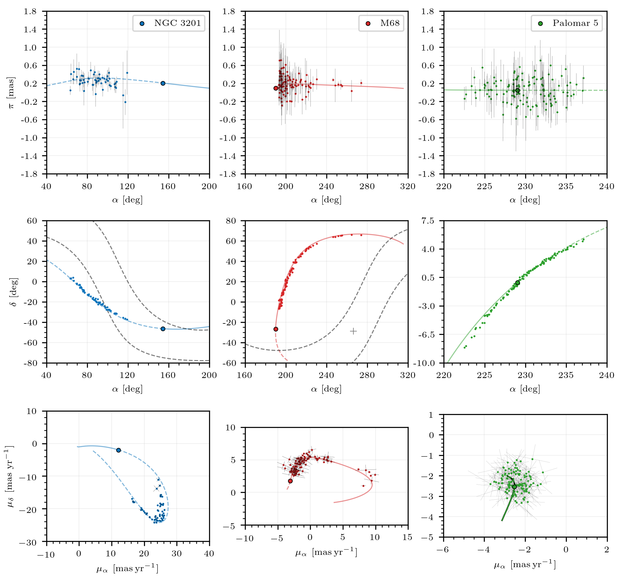
Figure 1: Phase-space position of stream stars from the GDR2 catalogue (points with error bars) for globular clusters NGC 3201 (blue), M68 (red), and Palomar 5 (green). Big dots show the current phase-space position of clusters and lines show their orbits forwards (solid) and backwards (dashed) during 60 Myr computed using the best-fitting orbit. Middle panels: The grey dashed lines mark the Milky Way disc limits at $b=\pm 15$ deg and the grey cross the Galactic centre.

The kinematics of NGC 3201 are specified in Table 1 and Table 2. We use the coordinates of Harris (1996, 2010), with negligible errors, and the heliocentric distance $r_{\rm h}$ from the same catalogue assuming a 2.3 per cent uncertainty. The radial velocity $v_{r}$ is from Baumgardt et al. (2019), who compile several measurements. We use proper motions from Vasiliev (2019b), based on GDR2 data. We take these properties as free parameters and take the quoted errors from the observations, listed in Table 1, as a prior assuming they are Gaussian.

We use the mean values of the phase-space coordinates of the cluster and a fiducial Galactic potential to simulate this stream (see Section 4). We assume that the mass and size of the cluster are fixed throughout the orbit. These properties are listed in Table 2. In Figure 2 we plot in Galactocentric Cartesian coordinates the simulated stars stripped from the cluster during the last 1.5 Gyr, and we highlight in blue the simulated stars that approximately fit with our selection of Gaia stars. We also indicate the position of NGC 3201 with a big blue dot. We see that the observed portion of the stream is located approximately from 10 to 13 kpc from the Galactic centre and very close to the Galactic disc, in the range -3 to 0 kpc.

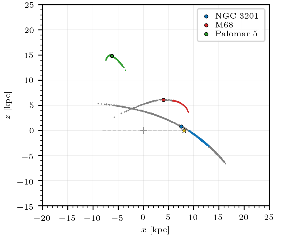
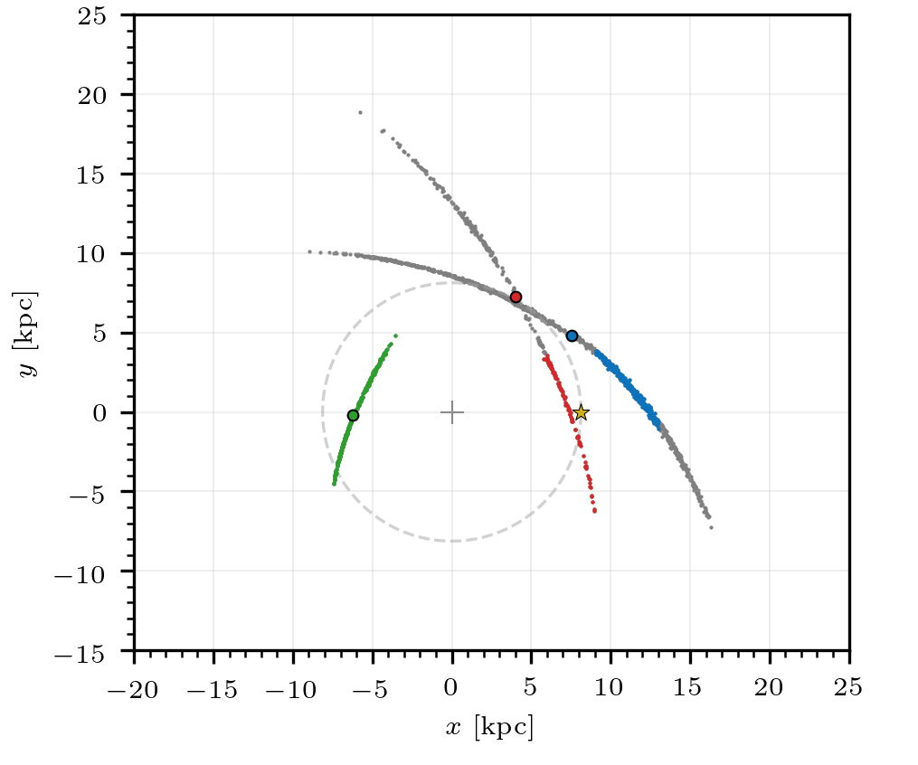
Figure 2: Simulated stream stars in Galactocentric coordinates, taking the stars stripped from the globular cluster during the last 1.5 Gyr for NGC 3201, and M68 and 4 Gyr for Palomar 5. The big dots show the current position of the globular clusters NGC 3201 (blue), M68 (red), and Palomar 5 (green). The coloured stars display approximately the section of the stream that fits with our Gaia selection plotted in Figure 1. The yellow star marks the Sun’s position and the grey dashed line shows its orbit assuming a circular motion. The grey cross marks the Galactic centre.

3.4.2 M68 stellar stream

The stellar stream associated with the globular cluster M68 (NGC 4590) is a long and thin structure that spans about 190 deg over the north Galactic hemisphere. This stream appears in Ibata et al. (2019b) named as Fjörm without being associated with M68. We use a 98-star subset of the stream candidates selected in PM19, corresponding to the stars with $\delta>-8$ deg. With this cut, we exclude stars located close to the Galactic disc, where the correct determination of stream members is uncertain due to the high level of foreground contamination. This selection includes stars along almost the entire leading arm of the stream which appears projected onto the halo. This section is described in detail in the Appendix A, and the final selection of stars we use to constrain the Galactic potential is shown in red in Figure 1. Most of these stars are located very close to the Sun at $\mathrel{\mathchoice{\raise 0.0pt\hbox{\scalebox{0.8}{\raise 0.0pt\hbox{$\displaystyle\sim$}}}}{\raise 0.0pt\hbox{\scalebox{0.8}{\raise 0.0pt\hbox{$\textstyle\sim$}}}}{\raise 0.0pt\hbox{\scalebox{0.8}{\raise 0.0pt\hbox{$\scriptstyle\sim$}}}}{\raise 0.0pt\hbox{\scalebox{0.8}{\raise 0.0pt\hbox{$\scriptscriptstyle\sim$}}}}}5.5$ kpc and have proper motions approximately in the range $[5\,\text{,}\,10]$ ${\rm mas\,yr}^{-1}$ making them easily identifiable with respect to the foreground. On the other hand, the section closer to the globular cluster and all the trailing arm are completely obscured by foreground stars, most of them belonging to the disc. Similarly to the stream of NGC 3201, we can assert the stream membership of each star by direct inspection of the stars passing a set of cuts in phase-space, colour and magnitude. This avoids possible biases towards the potential used by the statistical method in PM19.

For M68, we also take its sky coordinates as fixed parameters and the remaining phase-space coordinates as free parameters, assuming a 5 per cent of uncertainty for the heliocentric distance. We list their values in Table 2 and in Table 1 respectively. In Figure 2 we observe that the stream is located at about 9 to 12 kpc from the Galactic centre and about 4 to 6 kpc from the Galactic disc.

3.4.3 Palomar 5 stellar stream

The Palomar 5 tidal tails were discovered by Odenkirchen et al. (2001) by noticing an excess of stars around the globular cluster using photometric data provided by Sloan Digital Sky Survey. Further work improved the definition of the tidal tails and extended its length up to 23 deg in the sky (e.g. Carlberg et al., 2012). Its full phase-space distribution has been described by the identification of individual stars in the tidal stream (e.g. Kuzma et al., 2015; Ibata et al., 2016; Ibata et al., 2017), and improved using the GDR2 catalogue (Starkman et al., 2020; Price-Whelan et al., 2019).

In this paper, we use our selection of stream stars made following the method described in PM19. This method is based on a maximum-likelihood technique designed to distinguish stars compatible with being tidally stripped from a known globular cluster. These stream stars appear as an overdensity that is statistically identified when compared to a phase-space model of the Milky Way. The stars that most likely belong to the stream are selected by choosing those with the largest intersection with a phase-space density model of the stream. This model is computed numerically by optimising several free parameters to maximise the intersection between the stellar overdensity and the model. The free parameters include the potential model of the Galaxy and the heliocentric distance and velocity of the cluster within the constraints of the available observations. The stars selected using phase-space information are consistent with the recent observations of the Palomar 5 stream by Bonaca et al. (2020) using $grz$ photometry from DECaLS, which includes stars up to 24 mag. This ensures that our selection methodology does not introduce any bias that could affect the determination of the Galactic potential. Our final selection only includes the stars that are colour and magnitude compatible with the H-R diagram of the progenitor cluster. We show in green the 126 selected stars in Figure 1. We list the phase-space coordinates, colours and magnitudes and explain the details of the selection procedure in Appendix B. None of the selected stars has radial velocity in the GDR2 catalogue, but 15 of them match with stars with radial velocity measured by Ibata et al. (2017). We take their measurements, list them in Appendix B, and display the radial velocity in function of right ascension in Figure 3.

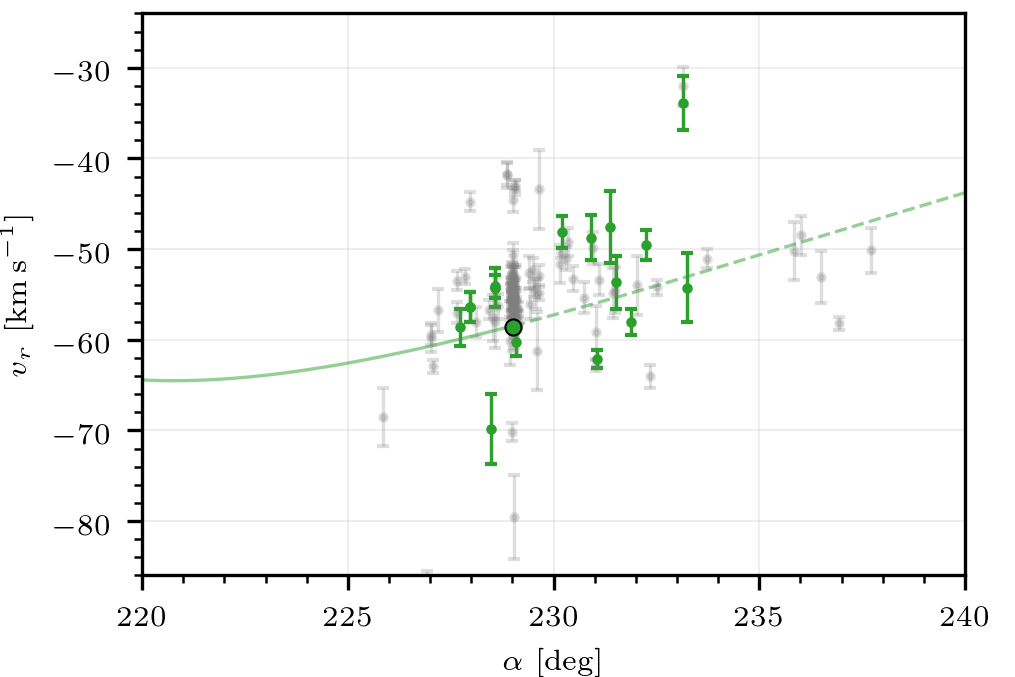
Figure 3: Right ascension and radial velocity of the stream stars of Palomar 5 from Ibata et al. (2017) (grey) with error bars. The green points mark the 15 stars that match with our Gaia selection. The big dot shows the current position of the cluster and the lines show its orbit forwards (solid) and backwards (dashed) during 60 Myr computed using the best-fitting values of the free parameters.

The Palomar 5 tidal stream is projected onto the halo just over the Galactic centre. Our selection covers about 16 deg in the sky, almost the entire stream. We observe a well-defined structure, with two long and thin arms connected to the globular cluster. The observations of Bonaca et al. (2020), show a low surface-brightness extension of $\mathrel{\mathchoice{\raise 0.0pt\hbox{\scalebox{0.8}{\raise 0.0pt\hbox{$\displaystyle\sim$}}}}{\raise 0.0pt\hbox{\scalebox{0.8}{\raise 0.0pt\hbox{$\textstyle\sim$}}}}{\raise 0.0pt\hbox{\scalebox{0.8}{\raise 0.0pt\hbox{$\scriptstyle\sim$}}}}{\raise 0.0pt\hbox{\scalebox{0.8}{\raise 0.0pt\hbox{$\scriptscriptstyle\sim$}}}}}10$ deg on the trailing arm. Our selection does not include this extension, as the Gaia $G\>\!\text{-band}$ magnitude limitation of $G<21$ mag makes it difficult to identify stars in the trailing arm faint extension. In the proper motion space, we observe a bunch of stars. We do not observe the long and thin shape of the stream because the internal dispersion of proper motions of the stream stars is much smaller than the Gaia observational uncertainties.

For the phase-space coordinates of Palomar 5, we take the values from the same references as in the previous cases (see Table 1 and 2), except for the heliocentric distance $r_{\rm h}$ taken from Price-Whelan et al. (2019). In general, the measurements of $r_{\rm h}$ approximately range from 20 to 23 kpc, here we use $20.6\pm 0.2$ kpc. The simulation of the stream (green dots in Figure 2) shows that the stream is located at about 13 to 17 kpc from the Galactic centre and about 12 to 15 kpc from the Galactic disc.

4 Statistical methodology

Given a set of free parameters $\theta$ and a set of observational measurements $d$, the posterior distribution of all parameters together $p\mbox{\footnotesize$(\theta|d)$}$ can be determined by the Bayes’ theorem:

$$p\mbox{\footnotesize$(\theta|d)$}=\frac{\mathcal{L}\mbox{\footnotesize$(d|\theta)$}\,p\mbox{\footnotesize$(\theta)$}}{p\mbox{\footnotesize$(d)$}}~{},$$ (14)

where $\mathcal{L}\mbox{\footnotesize$(d|\theta)$}$ is the likelihood function, $p\mbox{\footnotesize$(\theta)$}$ is the prior distribution of all the parameters, and $p\mbox{\footnotesize$(d)$}$ is a normalisation constant. In our model, we use 4 free parameters that characterise the position of the Sun, 12 for the potential of the Milky Way, and 4 for the phase-space position of each globular cluster. The free parameters, including their prior distribution functions, are described in Section 2 and listed in Table 1; those without a specified prior in this table are assigned a flat prior (with fixed limits added for numerical convenience that are broad enough to have no impact on our results). Parameters that are kept fixed are listed in Table 2.

The likelihood function is computed as the product of the likelihoods associated to each observational constraint. This is divided into two sets of data: first, the traditional dynamical constraints from equilibrium models of the Milky Way, consisting of a total of 5 measured variables described in Sections 2, 3.1, and 3.2 $(f_{\varSigma},M_{\rm b},M_{200},\mu_{l},{\rm and}\,K_{z})$, and the 38 values of the velocity rotation curve of Eilers et al. (2019), described in Section 3.3. For this, we assume a Gaussian distribution for all of these 43 variables and treat them independently, even though the 38 points of the rotation curve have a correlated error. We simply use error bars for the rotation curve that are larger than the purely statistical errors, by adding a systematic error of 3 per cent to each point, which roughly compensates for the error correlations.

The second data set are the observations of the 3 streams used in this paper. The data consist of a list of the phase-space coordinates of stars from the Gaia catalogue that have been selected as stream members. These include positions (with negligible errors), proper motions and parallaxes with the covariance matrix of the GDR2 measurement errors. In addition, radial velocities and their errors are available only for part of the stars of the Palomar 5 stream. We define the likelihood as the convolution of this measurement error distribution with a phase-space probability density model of the stellar stream (see Section 4.1). A more detailed definition of the likelihood function is explained in Appendix C.

To obtain the posterior distribution of the parameters of our model, we use the Metropolis-Hastings algorithm (MacKay, 2003), which is a Markov Chain Monte Carlo method that generates random samples following a probability density function. We use our own implementation of this method based on a Gaussian transition distribution with adjusted covariance matrix to maximize performance, and run 72 walkers initialized with a random position. The algorithm converges to a stationary set of samples after about $10^{5}$ steps for all parameters. These steps have been excluded to avoid a bias due to the random initial configuration, and the posterior distributions are drawn using the next $5\times 10^{5}$ steps of the chain. The halo parameters $\rho_{0}^{\rm h}$, $a_{1}$, and $\beta$ present an asymmetric posterior distribution with an extended tail towards large values (see Section 5.2). To ensure convergence, we limit the tail of the distributions with the boundaries of the uniform priors introduced in Section 2.3. We find the best-fitting values using a Nelder-Mead Simplex algorithm, and present the results in Section 5.

4.1 Phase-space model of the stellar stream

The phase-space probability density model of the stellar stream is constructed from simulated particles escaping from the globular cluster, modeled as a static Plummer potential orbiting the static Milky Way potential, subject to the tidal forces of the Galaxy. The model depends on the potential of the Milky Way, and the globular cluster mass, scale length and orbit.

Several methods have been developed to quickly simulate stellar streams. For example, the streak-line or particle-spray method avoids calculating the orbit of non-escaping stars (with the small time steps required in the cluster core) by releasing particles from the Lagrange points (e.g., Küpper et al., 2012). Alternatively, some methods rely on the simple structure of the stream in action-angle coordinates to create prescriptions for its phase-space structure (e.g., Bovy, 2014; Fardal et al., 2015). None of these methods is fast enough to compute a random sample large enough to adequately describe the posterior function (eq. 14) in a reasonable time with our computational resources, for the large variety of model parameters we want to examine.

For this reason, we do not simulate a stellar stream for each evaluation of the likelihood function. We do an accurate simulation only initially for fiducial parameter values, and then, we assume that the position and velocity dispersion of the stream with respect to the orbit of the progenitor do not change for small variations of the potential of the Galaxy and the phase-space location of the cluster. This assumption allows us to obtain an approximation of the stream phase-space structure without the computational cost of a numerical simulation. The initial simulation is carried out using the method described in PM19. The procedure we apply can be summarized as the following steps:

1. We compute the orbit of the globular cluster backwards in time during 1.5 Gyr for NGC 3201 and M68, and 4 Gyr for Palomar 5, starting from the present mean position and velocity. The time intervals are selected to match the size and length of the observed streams. The orbit is computed using the fiducial potential of the Galaxy defined in PM19.

2. We assume the globular cluster is initially in dynamical equilibrium and we randomly generate member stars using the equilibrium distribution function. In our case, we adopt a Plummer sphere, with the core radius $a_{\rm gc}$ and the cluster mass $M_{\rm gc}$ listed in Table 2 for the three globular clusters treated in this paper.

3. The orbits of the stars are computed starting from the initial position of the cluster centre computed in step (i) plus the distribution of relative positions and velocities computed in step (ii), up to the present time. The stars are treated as test particles moving in the fixed Galactic potential plus the Plummer model potential of constant mass moving along the previously computed orbit.

To compute the stream model for other parameters, we assume that the relative phase-space position of the stream stars with respect to the cluster orbit that we have computed with the fiducial model do not change for small variations of the orbit. We describe the exact procedure in Appendix D, and summarize it with the following steps:

1. We select a section of the cluster orbit corresponding to the cluster motion during 60 Myr for NGC 3201 and M68, and 40 Myr for Palomar 5, backwards and forwards in time with respect to the present location of the cluster. We define a Frenet-Serret trihedron on each point of the orbit. Each trihedron is a orto-normal vector basis defined by the normalised velocity and acceleration of the cluster and their perpendicular vector. This trihedron defines a reference frame with origin on its corresponding point of the orbit.

2. We assign to each star the trihedron located in the closest point of the orbit to the star, determined with a Euclidean distance. We store the position and velocity of the star with respect to the reference frame defined by its trihedron, and assume that this relative phase-space position does not significantly change for small variations of the cluster orbit. We also store the time position of the origin of the trihedron along the section of the orbit of the cluster.

3. For each new evaluation of the likelihood function for different parameters, we compute the new cluster orbit section over the same time period. In the time positions along the orbit previously stored, we compute their corresponding new trihedrons. Finally, we locate each star at the previously stored relative position and velocity with respect to new trihedrons.

This method neglects variations of the internal structure of the stream with respect to the cluster orbit, and changes the stream only due to the variation of the cluster orbit with the potential. Because the stream sections we study are thin and depart only at levels of few percent from the cluster orbit, we expect the error introduced by the method is negligible for our purpose in this paper (see Appendix D for a detailed justification of this assumption).

The positions and velocities of the test stars are finally converted to the heliocentric reference frame $(\pi,\delta,\alpha,v_{r},\mu_{\delta},\mu_{\alpha})$, and compared to the observational data. The phase-space probability density model of the stream is constructed in these coordinates using a kernel density estimation method, with a Gaussian distribution as a kernel. We locate the mean of the kernel distributions in the position of the simulated stream stars, and we compute their covariance matrices from the distribution of neighboring stream stars. We describe this method in detail in Appendix C.

5 Results for each model

The stellar streams of NGC 3201 and M68 are located at similar distances from the Galactic centre, covering a range from $r\mathrel{\mathchoice{\raise 0.0pt\hbox{\scalebox{0.8}{\raise 0.0pt\hbox{$\displaystyle\sim$}}}}{\raise 0.0pt\hbox{\scalebox{0.8}{\raise 0.0pt\hbox{$\textstyle\sim$}}}}{\raise 0.0pt\hbox{\scalebox{0.8}{\raise 0.0pt\hbox{$\scriptstyle\sim$}}}}{\raise 0.0pt\hbox{\scalebox{0.8}{\raise 0.0pt\hbox{$\scriptscriptstyle\sim$}}}}}6$ to 13 kpc. However, whereas the M68 stream is observed along an orbit portion that remains $\mathrel{\mathchoice{\raise 0.0pt\hbox{\scalebox{0.8}{\raise 0.0pt\hbox{$\displaystyle\sim$}}}}{\raise 0.0pt\hbox{\scalebox{0.8}{\raise 0.0pt\hbox{$\textstyle\sim$}}}}{\raise 0.0pt\hbox{\scalebox{0.8}{\raise 0.0pt\hbox{$\scriptstyle\sim$}}}}{\raise 0.0pt\hbox{\scalebox{0.8}{\raise 0.0pt\hbox{$\scriptscriptstyle\sim$}}}}}5$ kpc above the disc, the NGC 3201 stream traverses the disc from North to South. In contrast, the Palomar 5 stream is further away, $\mathrel{\mathchoice{\raise 0.0pt\hbox{\scalebox{0.8}{\raise 0.0pt\hbox{$\displaystyle\sim$}}}}{\raise 0.0pt\hbox{\scalebox{0.8}{\raise 0.0pt\hbox{$\textstyle\sim$}}}}{\raise 0.0pt\hbox{\scalebox{0.8}{\raise 0.0pt\hbox{$\scriptstyle\sim$}}}}{\raise 0.0pt\hbox{\scalebox{0.8}{\raise 0.0pt\hbox{$\scriptscriptstyle\sim$}}}}}$ 16 kpc from the centre and $\mathrel{\mathchoice{\raise 0.0pt\hbox{\scalebox{0.8}{\raise 0.0pt\hbox{$\displaystyle\sim$}}}}{\raise 0.0pt\hbox{\scalebox{0.8}{\raise 0.0pt\hbox{$\textstyle\sim$}}}}{\raise 0.0pt\hbox{\scalebox{0.8}{\raise 0.0pt\hbox{$\scriptstyle\sim$}}}}{\raise 0.0pt\hbox{\scalebox{0.8}{\raise 0.0pt\hbox{$\scriptscriptstyle\sim$}}}}}$ 14 kpc above the disc. Each stream is therefore probing different regions of the Galactic gravitational potential. To better understand the constraints provided by each stream, we first present the three mass models obtained by fitting each individual stream and then the model including all three streams together.

The results of our fits are listed in Table 6 in Appendix F, as the median value and 1$\sigma$ error of the posterior distribution marginalized over all other parameters, for each separate stream and for all streams together. Models with a single stream have a total of 20 free parameters. The model with all streams together requires 28 parameters because each stream includes four free parameters for the phase-space position of the globular cluster. We also list in the table results for other derived properties of the model, including rotation curve velocities at different radii, $f_{\Sigma}$, $\mu_{l}$, the masses of each Milky Way component, and several properties of the dark halo.

5.1 Consistency with model priors and other observational Data

Our main goal is to obtain new constraints on the mass distribution of the Milky Way halo, so we will discuss the results for the five parameters of our halo model: $\rho_{0}^{\rm h}$, $\alpha$, $\beta$, $a_{1}$, and in particular the axis ratio $q_{\rho}^{\rm h}$. Before this, we briefly comment on the consistency of all other parameters of our resulting fits with the priors that are imposed from observational determinations as discussed in Sections 2 and 3. As seen in Table 6, all parameters are generally within the errors of the priors, indicating that our models are fully consistent with all these observational constraints and can adequately fit them together with our new conditions from the stellar stream members. This gives us confidence on the results and errors obtained for the dark halo parameters.

We comment on some of the input parameters that show moderate discrepancies from the priors. For the Sgr A^∗ proper motion, all our best-fitting models differ by less than $1.8\sigma$ from the observed value in equation 12. The rotational velocity of our models at the Solar radius are $\Theta_{0}+V_{\scalebox{0.7}{$\odot$}}\mathrel{\mathchoice{\raise 0.0pt\hbox{\scalebox{0.8}{\raise 0.0pt\hbox{$\displaystyle\sim$}}}}{\raise 0.0pt\hbox{\scalebox{0.8}{\raise 0.0pt\hbox{$\textstyle\sim$}}}}{\raise 0.0pt\hbox{\scalebox{0.8}{\raise 0.0pt\hbox{$\scriptstyle\sim$}}}}{\raise 0.0pt\hbox{\scalebox{0.8}{\raise 0.0pt\hbox{$\scriptscriptstyle\sim$}}}}}245$ ${\rm km}\,{\rm s}^{-1}$, and $\Theta_{0}\mathrel{\mathchoice{\raise 0.0pt\hbox{\scalebox{0.8}{\raise 0.0pt\hbox{$\displaystyle\sim$}}}}{\raise 0.0pt\hbox{\scalebox{0.8}{\raise 0.0pt\hbox{$\textstyle\sim$}}}}{\raise 0.0pt\hbox{\scalebox{0.8}{\raise 0.0pt\hbox{$\scriptstyle\sim$}}}}{\raise 0.0pt\hbox{\scalebox{0.8}{\raise 0.0pt\hbox{$\scriptscriptstyle\sim$}}}}}231\,{\rm km}\,{\rm s}^{-1}$. Comparing these to other recent observational data, we see that our values are consistent with determinations of Reid et al. (2019) from parallaxes and proper motions of molecular masers associated with young high-mass stars: $\Theta_{0}+V_{\scalebox{0.7}{$\odot$}}=247\pm 4$ ${\rm km}\,{\rm s}^{-1}$ and $\Theta_{0}=236\pm 7$ ${\rm km}\,{\rm s}^{-1}$, for $R_{\scalebox{0.7}{$\odot$}}=8.15\pm 0.15$ kpc. They are also similar to Mróz et al. (2019), who used classical Cepheid proper motions and radial velocities from Gaia to infer: $\Theta_{0}+V_{\scalebox{0.7}{$\odot$}}=246.9\pm 1.6\,{\rm km}\,{\rm s}^{-1}$ and $\Theta_{0}=233.6\pm 2.8\,{\rm km}\,{\rm s}^{-1}$ for $R_{\scalebox{0.7}{$\odot$}}=8.122\pm 0.031$ kpc.

The parameters describing the bulge and disc of the Milky Way are mostly constrained by our priors described in Sections 2 and 3. The mass of the thin disc is an exception because the total disc mass is the main quantity that is degenerate with halo parameters, and it needs to be constrained by the combination of rotation curve data and our stream conditions (the thick disc contains less mass and is therefore less important for the potential, so it is mostly constrained by the priors). When the M68 stream is used individually, a larger disc mass by $\mathrel{\mathchoice{\raise 0.0pt\hbox{\scalebox{0.8}{\raise 0.0pt\hbox{$\displaystyle\sim$}}}}{\raise 0.0pt\hbox{\scalebox{0.8}{\raise 0.0pt\hbox{$\textstyle\sim$}}}}{\raise 0.0pt\hbox{\scalebox{0.8}{\raise 0.0pt\hbox{$\scriptstyle\sim$}}}}{\raise 0.0pt\hbox{\scalebox{0.8}{\raise 0.0pt\hbox{$\scriptscriptstyle\sim$}}}}}20$ per cent is required compared to the other two streams, which gives a total baryonic mass of $(8.3\pm 0.49)\!\times\!10^{10}$ M${}_{\scalebox{0.7}{$\odot$}}$. This value is significantly larger than the estimated in other models, e.g. $(6.43\pm 0.63)\!\times\!10^{10}$ M${}_{\scalebox{0.7}{$\odot$}}$ in McMillan (2011) or $(7.25^{+0.39}_{-0.68})\!\times\!10^{10}$ M${}_{\scalebox{0.7}{$\odot$}}$ in Cautun et al. (2020). The combination of M68 and Palomar 5 allows for reducing the parameter degeneracy of the disc mass with the oblateness and density profile of the halo dark matter. Including all the streams together, the resulting model also prefers a similarly high disc mass. Note that the increased disc mass of the models including the M68 stream, results in a larger vertical acceleration $K_{z}$, with a $2\sigma$ deviation from the observational prior we are using (eq. 13).

The phase-space locations of NGC 3201 and M68 are consistent with our priors from observations. The case of Palomar 5, on the other hand, shows discrepancies in the distance from the Sun $r_{\rm h}$ of $2.4\sigma$, and in the proper motion components of $1.5\sigma$ and $3.1\sigma$. This may partly be due to systematic errors in the distance measurement of $20.6\pm 0.2$ kpc in Price-Whelan et al. (2019) that we use as a prior. Our estimate of $21.19\pm 0.15$ kpc is closer to the literature average of $21.9\pm 0.5$ kpc from Baumgardt & Vasiliev (2021). The large shift preferred by our stream model fit in the proper motion of Palomar 5 may not be entirely explained by the positive correlation with $r_{\rm h}$, and may indicate an inability to obtain a sufficiently good fit to the stream with the model parameterization we have chosen.

5.1.1 Circular velocity curve

We plot the circular velocity curve of the Milky Way in the top panel of Figure 4. Solid lines give the total circular velocity of the three fitted models of each globular cluster stream, and dashed lines are the circular velocity of the baryonic mass models only. Black dots with error bars are the data taken from Eilers et al. (2019) with errors computed as described in Subsection 3.3. The bottom panel shows the residuals between models and data. There are no significant differences among the model rotation curves, which are all consistent with observations. Since the results of Eilers et al. (2019) do not extend to $R>25$ kpc, we include as brown dots with error bars the independent data of Huang et al. (2016), who use halo K giant stars (the HKG sample in the reference) extending from $\mathrel{\mathchoice{\raise 0.0pt\hbox{\scalebox{0.8}{\raise 0.0pt\hbox{$\displaystyle\sim$}}}}{\raise 0.0pt\hbox{\scalebox{0.8}{\raise 0.0pt\hbox{$\textstyle\sim$}}}}{\raise 0.0pt\hbox{\scalebox{0.8}{\raise 0.0pt\hbox{$\scriptstyle\sim$}}}}{\raise 0.0pt\hbox{\scalebox{0.8}{\raise 0.0pt\hbox{$\scriptscriptstyle\sim$}}}}}16$ to $100\,{\rm kpc}$, with typical uncertainty $\mathrel{\mathchoice{\raise 0.0pt\hbox{\scalebox{0.8}{\raise 0.0pt\hbox{$\displaystyle\sim$}}}}{\raise 0.0pt\hbox{\scalebox{0.8}{\raise 0.0pt\hbox{$\textstyle\sim$}}}}{\raise 0.0pt\hbox{\scalebox{0.8}{\raise 0.0pt\hbox{$\scriptstyle\sim$}}}}{\raise 0.0pt\hbox{\scalebox{0.8}{\raise 0.0pt\hbox{$\scriptscriptstyle\sim$}}}}}20$ ${\rm km}\,{\rm s}^{-1}$. These data are also in reasonably good agreement with our models at $R\mathrel{\mathchoice{\raise 0.0pt\hbox{\scalebox{0.8}{\raise 0.0pt\hbox{$\displaystyle\gtrsim$}}}}{\raise 0.0pt\hbox{\scalebox{0.8}{\raise 0.0pt\hbox{$\textstyle\gtrsim$}}}}{\raise 0.0pt\hbox{\scalebox{0.8}{\raise 0.0pt\hbox{$\scriptstyle\gtrsim$}}}}{\raise 0.0pt\hbox{\scalebox{0.8}{\raise 0.0pt\hbox{$\scriptscriptstyle\gtrsim$}}}}}30\,{\rm kpc}$, in particular with the magnitude of the slight decline of the circular velocity at these large radii.

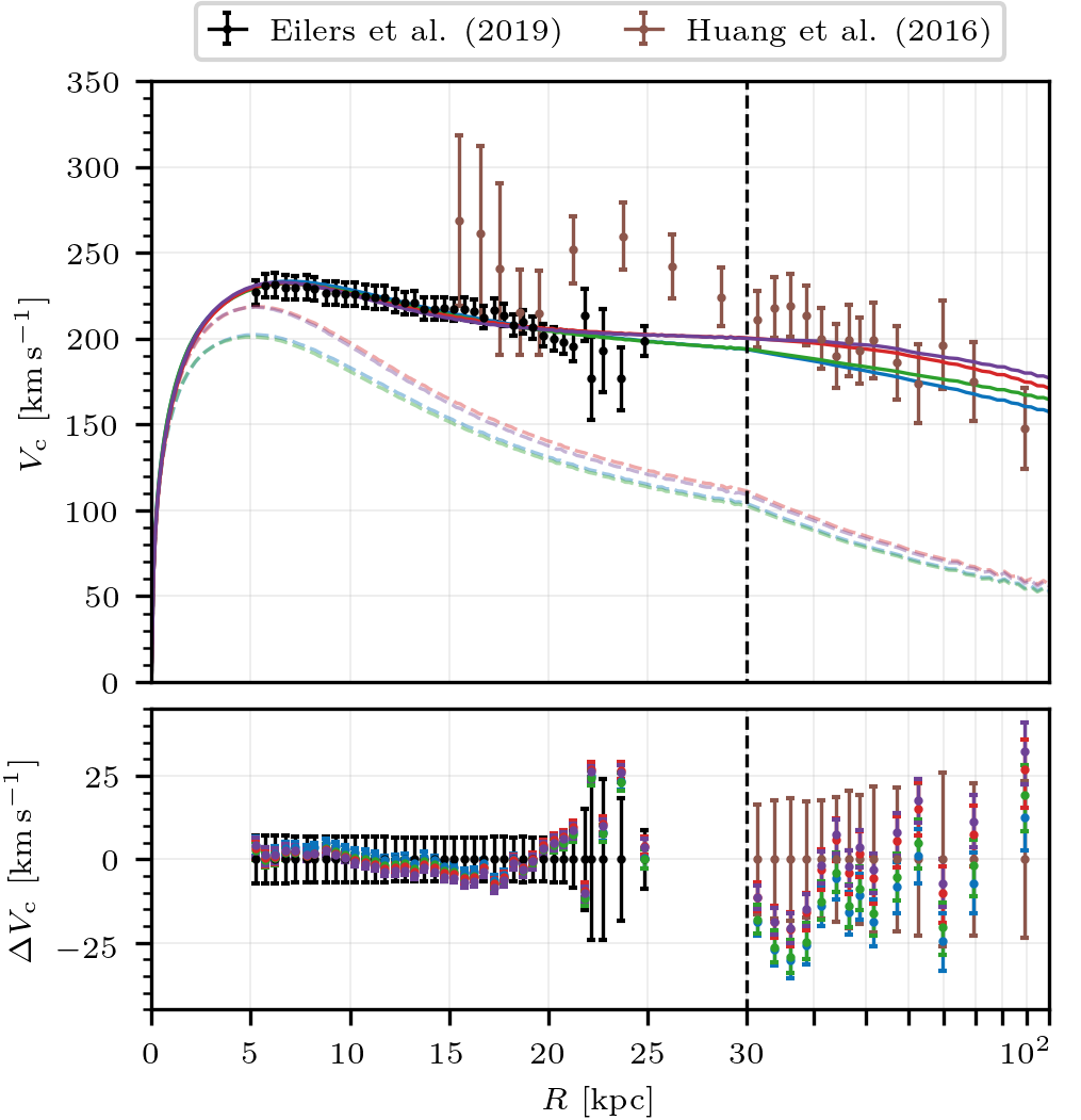
Figure 4: Circular velocity curve of the Milky Way. Top panel: Solid lines are best-fitting models rotation curves of the single streams of NGC 3201 (blue), M68 (red), Palomar 5 (green), and all streams together (purple). Dashed lines are baryonic component contributions. Black dots with error bars are rotation curve data by Eilers et al. (2019), with errors computed as described in Subsection 3.3, and brown dots with error bars are from halo K giant velocities from Huang et al. (2016) (from their HKG sample). Horizontal scale changes from linear to logarithmic at dashed vertical black line. Bottom panel: Residuals between models and observational data.

5.2 Dark matter halo results: individual streams

We now present the main results of the paper on the dark matter halo parameters fitting for each individual stream in this subsection, and all three streams together in the next subsection. In Figure 5, we present the posterior distribution function marginalized over each pair of halo parameters (contour panels) and each individual parameter (colored curves) for each model. We use the same color code as before. We also include the Pearson correlation coefficient between the two marginalised parameters in the legend of each panel.

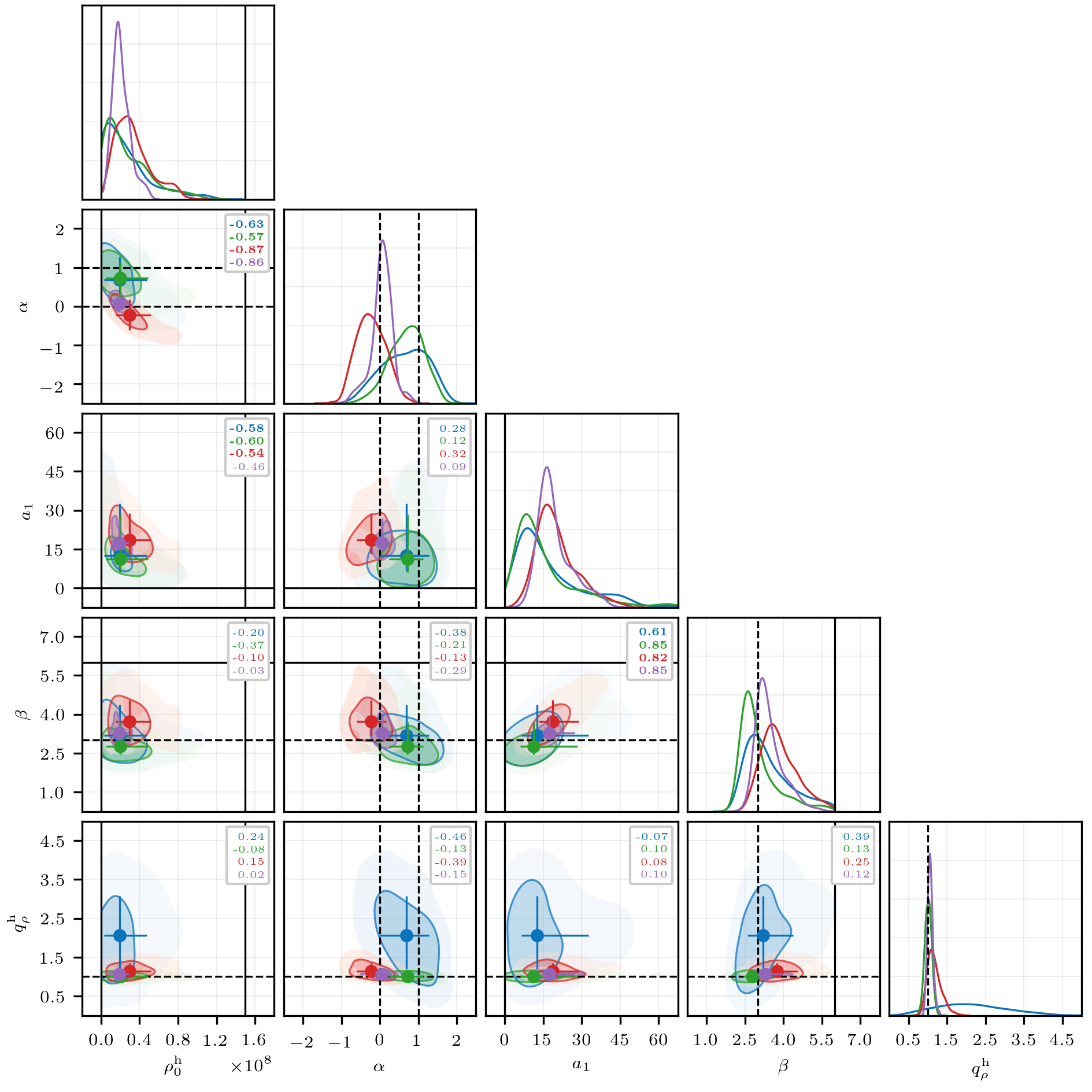
Figure 5: Halo parameters corner plot: posterior distributions marginalised over all parameter pairs (bright shaded areas with solid contours are $1\sigma$ level, faint shaded areas are $2\sigma$ level), and each single parameter (curves), for the stream models of NGC 3201 (blue), M68 (red), Palomar 5 (green), and all streams together (purple). Dots: distribution medians. Solid black lines: limits of uniform priors, when present in displayed intervals. Dashed lines: Flat and NFW inner and outer halo slopes ($\alpha=0,1$, $\beta=3$), and spherical configuration ($q_{\rho}^{\rm h}=1$). Legend of each panel shows Pearson correlation coefficients.

We first comment on the halo density profile preferred by our models. In general, all the models demand a flatter density core in the region where baryons dominate ($R\mathrel{\mathchoice{\raise 0.0pt\hbox{\scalebox{0.8}{\raise 0.0pt\hbox{$\displaystyle\lesssim$}}}}{\raise 0.0pt\hbox{\scalebox{0.8}{\raise 0.0pt\hbox{$\textstyle\lesssim$}}}}{\raise 0.0pt\hbox{\scalebox{0.8}{\raise 0.0pt\hbox{$\scriptstyle\lesssim$}}}}{\raise 0.0pt\hbox{\scalebox{0.8}{\raise 0.0pt\hbox{$\scriptscriptstyle\lesssim$}}}}}15\,{\rm kpc}$) than the NFW density profile. This is reflected in the small values of the inner slope $\alpha$ and in our large core radii $a_{1}\mathrel{\mathchoice{\raise 0.0pt\hbox{\scalebox{0.8}{\raise 0.0pt\hbox{$\displaystyle\sim$}}}}{\raise 0.0pt\hbox{\scalebox{0.8}{\raise 0.0pt\hbox{$\textstyle\sim$}}}}{\raise 0.0pt\hbox{\scalebox{0.8}{\raise 0.0pt\hbox{$\scriptstyle\sim$}}}}{\raise 0.0pt\hbox{\scalebox{0.8}{\raise 0.0pt\hbox{$\scriptscriptstyle\sim$}}}}}15\,{\rm kpc}$ (see Table 6). For NGC 3201 and Palomar 5, $\alpha$ is consistent with $\mathrel{\mathchoice{\raise 0.0pt\hbox{\scalebox{0.8}{\raise 0.0pt\hbox{$\displaystyle\sim$}}}}{\raise 0.0pt\hbox{\scalebox{0.8}{\raise 0.0pt\hbox{$\textstyle\sim$}}}}{\raise 0.0pt\hbox{\scalebox{0.8}{\raise 0.0pt\hbox{$\scriptstyle\sim$}}}}{\raise 0.0pt\hbox{\scalebox{0.8}{\raise 0.0pt\hbox{$\scriptscriptstyle\sim$}}}}}0.7$, and for the M68 stream, the preferred $\alpha$ is actually negative. This result reflects the preference for a more massive disc in this model (implying less dark matter at small radii). A negative $\alpha$ is of course not physical, and is simply indicating the preference for the model for a reduced dark matter density in the central region.

The outer slope $\beta$ is highly correlated with the total mass $M_{200}$ and $a_{1}$ in all our models, and it is nearly unconstrained by the stellar streams and rotation curve data. The outer halo density profile is adjusted to fit the constraint of the total mass imposed by the satellite velocities (eq. 10). The obtained value is about $\beta=3$ in the three individual stream models.

It is also of interest that the local dark matter density in our models, $\rho_{\rm h}\mbox{\footnotesize$(R_{\scalebox{0.7}{$\odot$}})$}$, is lower than the value usually estimated for dark matter detection of $\mathrel{\mathchoice{\raise 0.0pt\hbox{\scalebox{0.8}{\raise 0.0pt\hbox{$\displaystyle\sim$}}}}{\raise 0.0pt\hbox{\scalebox{0.8}{\raise 0.0pt\hbox{$\textstyle\sim$}}}}{\raise 0.0pt\hbox{\scalebox{0.8}{\raise 0.0pt\hbox{$\scriptstyle\sim$}}}}{\raise 0.0pt\hbox{\scalebox{0.8}{\raise 0.0pt\hbox{$\scriptscriptstyle\sim$}}}}}0.4$ ${\rm GeV\,cm}^{-3}$ (see, e.g., de Salas, 2020). The models for NGC 3201 and M68 favor $\rho_{\rm h}\mbox{\footnotesize$(R_{\scalebox{0.7}{$\odot$}})$}\mathrel{\mathchoice{\raise 0.0pt\hbox{\scalebox{0.8}{\raise 0.0pt\hbox{$\displaystyle\sim$}}}}{\raise 0.0pt\hbox{\scalebox{0.8}{\raise 0.0pt\hbox{$\textstyle\sim$}}}}{\raise 0.0pt\hbox{\scalebox{0.8}{\raise 0.0pt\hbox{$\scriptstyle\sim$}}}}{\raise 0.0pt\hbox{\scalebox{0.8}{\raise 0.0pt\hbox{$\scriptscriptstyle\sim$}}}}}0.2$ GeV cm^-3, and the more spherical halo of the Palomar 5 model favors a slightly larger value, $\rho_{\rm h}\mbox{\footnotesize$(R_{\scalebox{0.7}{$\odot$}})$}\mathrel{\mathchoice{\raise 0.0pt\hbox{\scalebox{0.8}{\raise 0.0pt\hbox{$\displaystyle\sim$}}}}{\raise 0.0pt\hbox{\scalebox{0.8}{\raise 0.0pt\hbox{$\textstyle\sim$}}}}{\raise 0.0pt\hbox{\scalebox{0.8}{\raise 0.0pt\hbox{$\scriptstyle\sim$}}}}{\raise 0.0pt\hbox{\scalebox{0.8}{\raise 0.0pt\hbox{$\scriptscriptstyle\sim$}}}}}0.28$ GeV cm^-3. $\rho_{\rm h}\mbox{\footnotesize$(R_{\scalebox{0.7}{$\odot$}})$}$ depend on several parameters, but mainly correlate with the axis ratio. In general, spherical halos are assumed, which explains the discrepancy with our models requiring prolate halos.

5.2.1 Dark halo axis ratio

We now discuss the result on the main focus of our paper, the dark halo axis ratio $q_{\rho}^{\rm h}$. Its marginalised probability density function is shown in Figure 6 as a histogram, with the median and $1\sigma$ dispersion indicated in the legend. We also show the best-fitting log-Normal distributions as solid lines, and detail their parameters and additional distribution properties in Appendix E. Two-parameter marginalized distribution are shown for the axis ratio together with the total baryonic mass $M_{{\rm bar}}$, and the local dark matter halo density $\rho_{\rm h}\mbox{\footnotesize$(R_{\scalebox{0.7}{$\odot$}})$}$, in the two panels in Figure 7, with the same color and legend codes as in Figure 5.

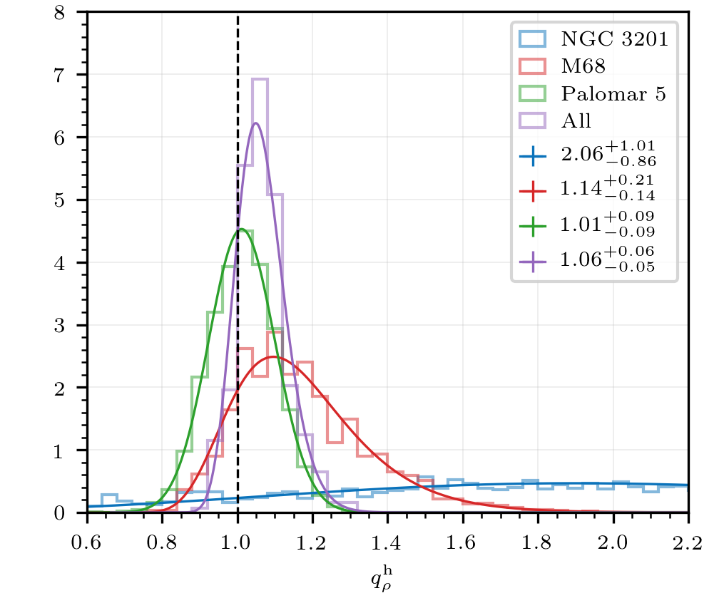
Figure 6: Posterior distribution of the halo axis ratio $q_{\rho}^{\rm h}$ in the stream models of NGC 3201 (blue), M68 (red), Palomar 5 (green), and all streams together (purple), shown as histograms obtained from random samples. Median and $1\sigma$ levels are shown in the legend, and the best-fitting log-Normals are shown as solid lines (see Appendix E). Spherical halo ($q_{\rho}^{\rm h}=1$) is marked as vertical dashed line.

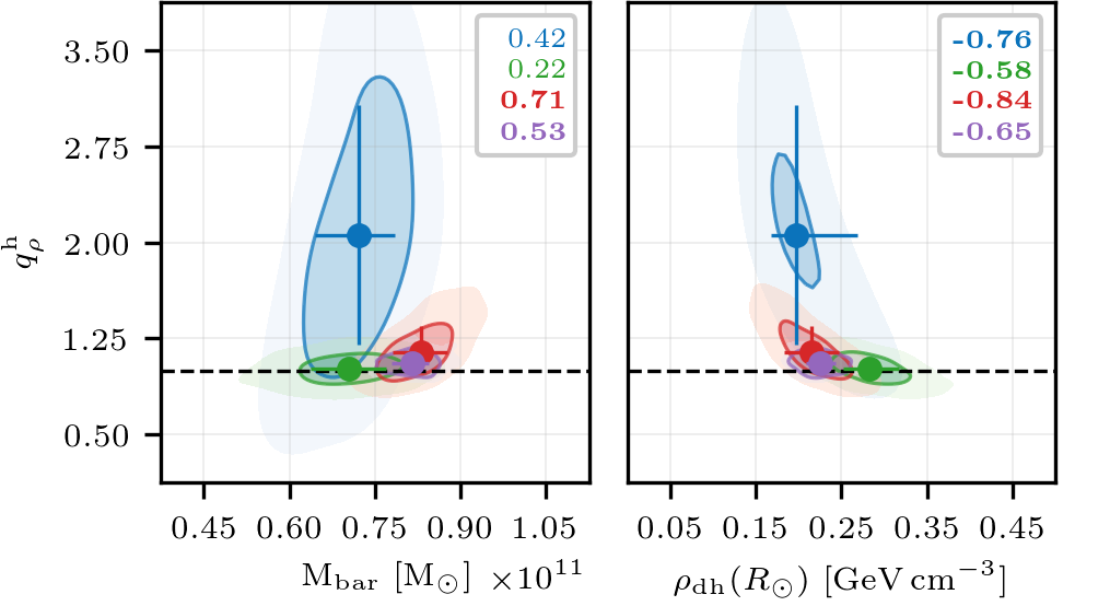
Figure 7: Same as Figure 5, for the axis ratio distribution together with the baryonic mass $M_{{\rm bar}}$ (left-hand panel) and the local dark matter density $\rho_{\rm h}(R_{\scalebox{0.7}{$\odot$}})$ (right-hand panel).

The stream generated by NGC 3201 does not help much constraining this parameter, giving a large error $q_{\rho}^{\rm h}=2.06\pm 0.93$, with a rather asymmetric distribution that favors a prolate halo. This wide distribution is a consequence of the observed short section of the stream being located close to the pericentre, and with an equatorial projection that makes the stellar distribution insensitive to the variation of the axis ratio. Palomar 5 yields a much more powerful constraint of $q_{\rho}^{\rm h}=1.01\pm 0.09$, implying the halo is rather close to spherical, without a dependence on the stellar mass. For M68 we obtain $q_{\rho}^{\rm h}=1.14^{+0.21}_{-0.14}$, in good agreement with Palomar 5 even though the streams explore very different regions of the gravitational potential. The M68 stream is compatible with a spherical halo but favoring a prolate one. For the M68 stream model, a more spherical halo is correlated with a lower stellar mass (see right panel of Figure 7), to compensate the acceleration on the stream (which has its best measured part passing 5 kpc above the disc) produced by each component. There is no significant correlation between the axis ratio and the other halo parameters for any of the streams. For Palomar 5, the main correlation appears with the heliocentric distance of the cluster which, at the same time, has a weak correlation with the proper motion of the cluster.

5.3 Model with all streams together

When all three streams are included together in the model, the halo shape is better constrained using data over a larger region. The M68 stream improves the constraint on the disc mass, which is larger than the best fit for the other two streams (see Section 5.1). The three stream model results in $M_{\rm d}^{\rm n}=(6.07\pm 0.39)\!\times\!10^{10}$ and $M_{{\rm bar}}=(8.01\pm 0.38)\!\times\!10^{10}$ ${\rm M}_{\scalebox{0.7}{$\odot$}}$, similar to the results using only the M68 stream. This gives a vertical gravitational acceleration at the solar radius $\mathrel{\mathchoice{\raise 0.0pt\hbox{\scalebox{0.8}{\raise 0.0pt\hbox{$\displaystyle\sim$}}}}{\raise 0.0pt\hbox{\scalebox{0.8}{\raise 0.0pt\hbox{$\textstyle\sim$}}}}{\raise 0.0pt\hbox{\scalebox{0.8}{\raise 0.0pt\hbox{$\scriptstyle\sim$}}}}{\raise 0.0pt\hbox{\scalebox{0.8}{\raise 0.0pt\hbox{$\scriptscriptstyle\sim$}}}}}1.8\sigma$ above the prior from other observational constraints (eq. 13), and also a transverse velocity of Sgr A^∗ at $-1.8\sigma$ from the observation (eq. 12), similarly to the Palomar 5 case as discussed above. The implied LSR velocity, $\Theta_{0}=230.67\pm 1.55$ ${\rm km}\,{\rm s}^{-1}$, and transverse solar velocity $\Theta_{0}+V_{\scalebox{0.7}{$\odot$}}=244.38\pm 0.91\,{\rm km}\,{\rm s}^{-1}$, are again consistent with other measurements as discussed in Section 5.1. The rotation curve is consistent with observations, with slightly larger velocities at large radius compared to single stream models. This is related to the larger total dark halo mass of the three-stream model, $M_{200}^{\rm h}=(1.08\pm 0.22)\!\times\!10^{12}$ ${\rm M}_{\scalebox{0.7}{$\odot$}}$, $\mathrel{\mathchoice{\raise 0.0pt\hbox{\scalebox{0.8}{\raise 0.0pt\hbox{$\displaystyle\sim$}}}}{\raise 0.0pt\hbox{\scalebox{0.8}{\raise 0.0pt\hbox{$\textstyle\sim$}}}}{\raise 0.0pt\hbox{\scalebox{0.8}{\raise 0.0pt\hbox{$\scriptstyle\sim$}}}}{\raise 0.0pt\hbox{\scalebox{0.8}{\raise 0.0pt\hbox{$\scriptscriptstyle\sim$}}}}}$ 14 per cent larger than the previous models.

The three stream model provides an improved constraint on the density profile, with a similar conclusion of a flat inner profile, with $\alpha=0.06\pm 0.22$, within a large core of about $a_{1}=17^{+10}_{-3}$ kpc. The core radius is nevertheless strongly correlated with the outer slope $\beta=3.3^{+0.7}_{-0.3}$. The result for the axis ratio is $q_{\rho}^{\rm h}=1.06\pm 0.06$, again consistent with spherical and slightly favoring a small deviation toward a prolate halo. As with all other streams separately, there is no significant correlation between the axis ratio and the other halo parameters. A larger baryonic mass, as preferred by the M68 stream, is what biases the axis ratio toward a more prolate halo.

6 Discussion

6.1 Comparison to previous studies: observations

Several studies have been made of the Milky Way dark matter halo shape using parametric models for the mass distribution constrained by observational data, and comparing this to predictions from cosmological simulations of Milky Way-like galaxies taking into account baryonic effects. In this subsection, we review these studies focusing on the halo axis ratio and compare them to our results.

We consider studies of the Milky Way halo shape based on axisymmetric analytic models consistent with dynamical equilibrium, with the symmetry axis perpendicular to the Galactic disc. Many studies adopt a NFW density profile for the halo, or a generalised version where the inner and outer power-law slopes are free (gNFW). In other models, the halo potential is assumed to follow the axisymmetric logarithmic potential, $\Phi_{h}=\log[R^{2}+(z/q_{\Phi}^{\rm h})^{2}+r_{c}^{2}]$, with a core radius $r_{c}$. Results from this type of studies are shown in Figure 8 for the halo density axis ratio $q_{\rho}^{\rm h}$ (red) and the halo potential axis ratio $q_{\Phi}^{\rm h}$ (black), with their quoted error bars. The studies are grouped according to the main source of observational data (in boldface), with the halo model that is used indicated under each reference. The dashed vertical line indicates the spherical case ($q^{\rm h}=1$).

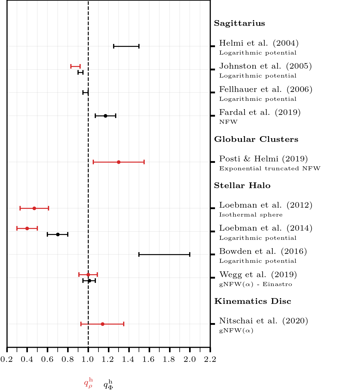
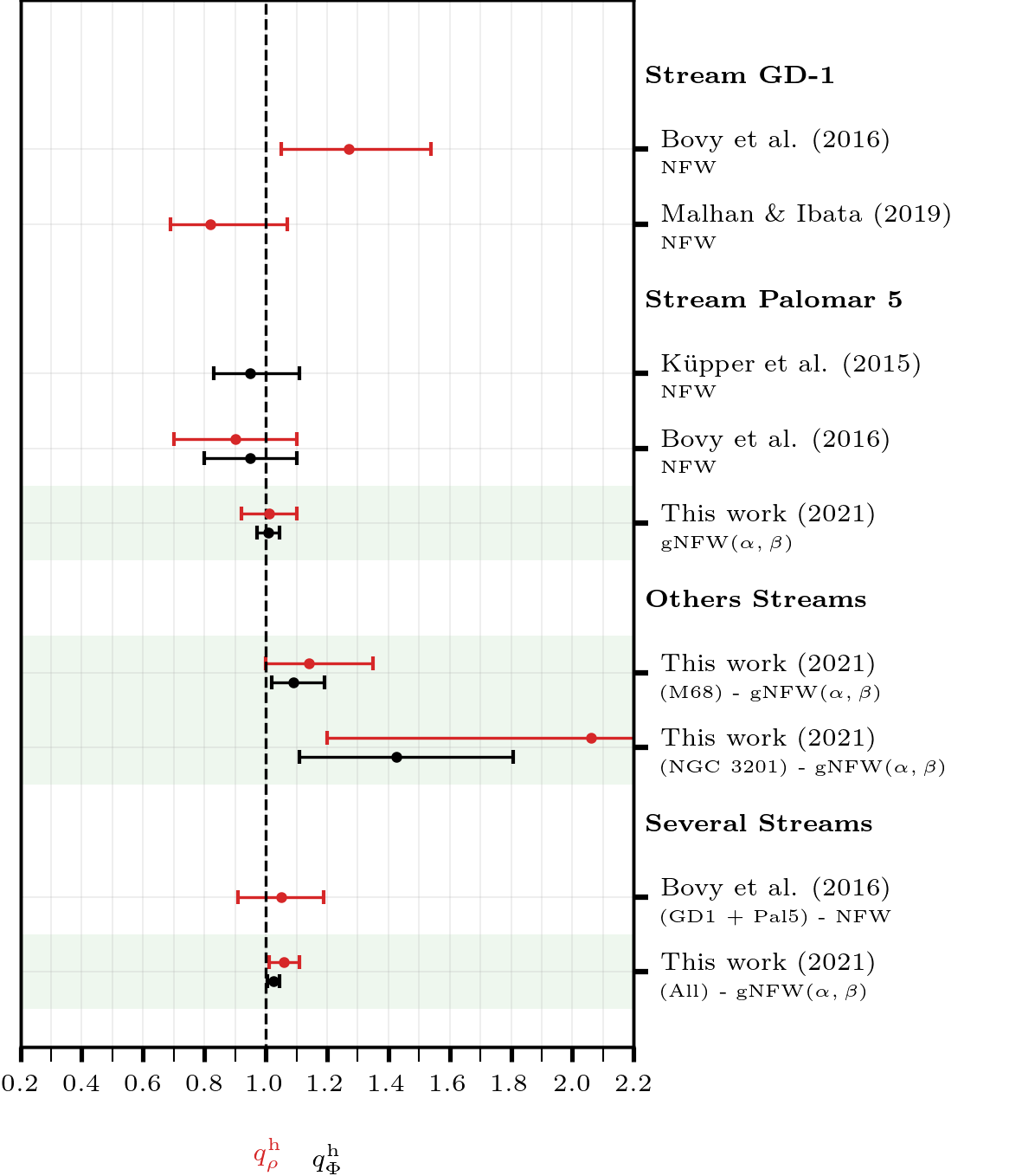
Figure 8: A list of estimates of the axis ratio of the dark matter halo density, $q_{\rho}^{\rm h}$ (red), and potential, $q_{\Phi}^{\rm h}$ (black), comparing our work and previous ones, grouped according to main source of observational data (in boldface). The halo model used is indicated under the reference, including the slope values for gNFW in parentheses. Dots are mean or median value as stated in the source, and bars are $1\sigma$ deviations (dots are absent when the result is reported as an interval). Vertical dashed line marks the spherical case and green shaded regions highlight our estimates.

Early studies did not converge to a consistent picture. Some studies using the Sagittarius stellar stream proposed triaxial shapes (Law et al., 2009; Law & Majewski, 2010; Deg & Widrow, 2013), but were criticised for their instability and incompatibility with constraints from Palomar 5 or Sagittarius’s tidal streams (see e.g. Ibata et al., 2013; Debattista et al., 2013; Belokurov et al., 2014; Pearson et al., 2015), and we exclude them in Figure 8. Using a sample of carbon stars, Ibata et al. (2001) noticed that the Sagittarius stream is observed as a Great Circle, indicating that the dark halo is most likely nearly spherical at $16<r<60$ kpc. Also based on Sagittarius stream, Helmi (2004) obtained a prolate halo, while Johnston et al. (2005) and Fellhauer et al. (2006) obtained a shape much closer to spherical and slightly oblate. Likewise, using equilibrium models of halo stars, Loebman et al. (2012, 2014) found an oblate dark matter halo while Bowden et al. (2016) obtained a prolate one.

On the other hand, recent studies offer a more consistent picture, indicating a nearly spherical halo, or a slightly prolate shape. Using the Sagittarius stream mapped with RR Lyrae from Pan-STARRS1, Fardal et al. (2019) found $q^{\rm h}_{\Phi}=1.17\pm 0.1$. This is not far from the result of Wegg et al. (2019) using RR Lyrae halo stars in the radius range $r\mathrel{\mathchoice{\raise 0.0pt\hbox{\scalebox{0.8}{\raise 0.0pt\hbox{$\displaystyle\sim$}}}}{\raise 0.0pt\hbox{\scalebox{0.8}{\raise 0.0pt\hbox{$\textstyle\sim$}}}}{\raise 0.0pt\hbox{\scalebox{0.8}{\raise 0.0pt\hbox{$\scriptstyle\sim$}}}}{\raise 0.0pt\hbox{\scalebox{0.8}{\raise 0.0pt\hbox{$\scriptscriptstyle\sim$}}}}}2$ to $20$ kpc, who conclude that the halo is spherical with $q^{\rm h}_{\rho}=1\pm 0.09$ (these authors obtain the same result assuming a gNFW or a Einastro halo radial profile). The study of Hattori et al. (2021) assumes an equilibrium distribution function of globular clusters to infer the halo axis ratio. The distribution is computed in angle-action framework using the Agama package (Vasiliev, 2019a) which is limited to spherical-oblate axisymmetric potentials. They found $0.963<q^{\rm h}_{\rho}$, strongly disfavouring a flattened dark matter halo. We note also that Hattori & Valluri (2020) favor a halo axis ratio near $q_{\rho}^{\rm h}\simeq 1.5$ using a hypervelocity star and assuming that it was ejected from the Galactic centre. In addition, Nitschai et al. (2020) use disc kinematic data at $R\mathrel{\mathchoice{\raise 0.0pt\hbox{\scalebox{0.8}{\raise 0.0pt\hbox{$\displaystyle\sim$}}}}{\raise 0.0pt\hbox{\scalebox{0.8}{\raise 0.0pt\hbox{$\textstyle\sim$}}}}{\raise 0.0pt\hbox{\scalebox{0.8}{\raise 0.0pt\hbox{$\scriptstyle\sim$}}}}{\raise 0.0pt\hbox{\scalebox{0.8}{\raise 0.0pt\hbox{$\scriptscriptstyle\sim$}}}}}4$ to 12 kpc and a vertical height $|z|\mathrel{\mathchoice{\raise 0.0pt\hbox{\scalebox{0.8}{\raise 0.0pt\hbox{$\displaystyle\sim$}}}}{\raise 0.0pt\hbox{\scalebox{0.8}{\raise 0.0pt\hbox{$\textstyle\sim$}}}}{\raise 0.0pt\hbox{\scalebox{0.8}{\raise 0.0pt\hbox{$\scriptstyle\sim$}}}}{\raise 0.0pt\hbox{\scalebox{0.8}{\raise 0.0pt\hbox{$\scriptscriptstyle\sim$}}}}}2\,{\rm kpc}$, favoring also a slightly prolate halo with $q^{\rm h}_{\rho}=1.14\pm 0.21$, although their error bar is also large.

In general, studies that have used stellar streams are all consistent with each other. Their results are plotted in the right-hand panel of Figure 8, along with our estimates highlighted with a light green shade. We do not include the first studies using the GD-1 stellar stream (Koposov et al., 2010; Bowden et al., 2015) because they did not constrain the dark matter halo directly but the overall potential of the Galaxy. Using the GD-1 stream, Bovy et al. (2016) find $q_{\rho}^{\rm h}\simeq 1.27\pm 0.27$, but Malhan & Ibata (2019) obtain $q_{\rho}^{\rm h}=0.82^{+0.25}_{-0.13}$. The latter study uses better constraints from a larger number of stars from the GDR2 catalogue; nevertheless, the results still have a large error bar and are both compatible with a spherical halo.

6.2 Comparison to our study based on stellar streams

We compare now these results based on the GD-1 stream with our models of the M68 and NGC 3201 streams. The observed sections of the GD-1 and M68 streams are at similar distances above the Galactic disc, and even though the M68 stellar stream is $\mathrel{\mathchoice{\raise 0.0pt\hbox{\scalebox{0.8}{\raise 0.0pt\hbox{$\displaystyle\sim$}}}}{\raise 0.0pt\hbox{\scalebox{0.8}{\raise 0.0pt\hbox{$\textstyle\sim$}}}}{\raise 0.0pt\hbox{\scalebox{0.8}{\raise 0.0pt\hbox{$\scriptstyle\sim$}}}}{\raise 0.0pt\hbox{\scalebox{0.8}{\raise 0.0pt\hbox{$\scriptscriptstyle\sim$}}}}}$ 5 kpc closer to the Galactic centre than GD-1, they are still sensitive to a similar radial range of the dark halo shape. Our estimate favours a prolate halo but is compatible with a spherical shape, in better agreement with Bovy et al. (2016) but not incompatible with Malhan & Ibata (2019). In the case of the NGC 3201 stream, located at similar distance from the Galactic centre as GD-1 but closer to the disc plane, our error bar using only NGC 3201 is very large but still favours a prolate halo, compatible with M68 and Bovy et al. (2016).

The case of the Palomar 5 stream is particularly interesting, because its position, far above the disc at a larger distance from the Galactic centre, makes it a better probe of the dark halo shape. Küpper et al. (2015) carried out a study using sky coordinates and line-of-sight velocities of several members of this stream. Modeling the Milky Way with a Miyamoto-Nagai disc potential and a NFW halo density profile, and using a Bayesian framework developed by Bonaca et al. (2014), they infer $q_{\Phi}^{\rm h}=0.95^{+0.16}_{-0.12}$. At the same time, Bovy et al. (2016) use a similar model and data but a different stream-fitting methodology based on action-angle modelling introduced in Bovy (2014), obtaining $q_{\rho}^{\rm h}=0.9\pm 0.2$. The latter authors also combine the Palomar 5 stream with GD-1 to obtain the improved constraint $q_{\Phi}^{\rm h}=1.05\pm 0.14$.

These estimates agree within the quoted observational errors, and they are also compatible with our result for Palomar 5 alone, $q_{\rho}^{\rm h}=1.01\pm 0.09$. Our error bar is smaller, even though our halo model has more free parameters. The likely reason is that we have a larger sample of stars with five phase-space parameters measured by GDR2 and 15 stars with radial velocity. We conclude that our measurements are fully consistent with these previous studies, including our combined result from the three streams we use, $q_{\rho}^{\rm h}=1.06\pm 0.06$. All of them favour a halo that is close to spherical, eliminating in particular the possibility of a highly oblate halo. This conclusion applies to the range of radii probed by these streams, $10\mathrel{\mathchoice{\raise 0.0pt\hbox{\scalebox{0.8}{\raise 0.0pt\hbox{$\displaystyle\lesssim$}}}}{\raise 0.0pt\hbox{\scalebox{0.8}{\raise 0.0pt\hbox{$\textstyle\lesssim$}}}}{\raise 0.0pt\hbox{\scalebox{0.8}{\raise 0.0pt\hbox{$\scriptstyle\lesssim$}}}}{\raise 0.0pt\hbox{\scalebox{0.8}{\raise 0.0pt\hbox{$\scriptscriptstyle\lesssim$}}}}}r\mathrel{\mathchoice{\raise 0.0pt\hbox{\scalebox{0.8}{\raise 0.0pt\hbox{$\displaystyle\lesssim$}}}}{\raise 0.0pt\hbox{\scalebox{0.8}{\raise 0.0pt\hbox{$\textstyle\lesssim$}}}}{\raise 0.0pt\hbox{\scalebox{0.8}{\raise 0.0pt\hbox{$\scriptstyle\lesssim$}}}}{\raise 0.0pt\hbox{\scalebox{0.8}{\raise 0.0pt\hbox{$\scriptscriptstyle\lesssim$}}}}}20\,{\rm kpc}$.

6.3 Predictions from cosmological simulations

Cosmological simulations including only dark matter predict that the gravitational evolution of random initial fluctuations should lead to highly triaxial halos. However, when models of the behaviour of the baryonic components are included, with the complexities of disc and bar formation near the centre, halos are found to generally become more rounded owing to the accumulation of a central mass dominated by baryons. In fact, the potential of a triaxial halo is generally supported by highly populated box orbits that are aligned along the long axis of the potential. When a concentrated structure grows at the centre, dark matter particles in initially box orbits can be scattered in random directions when passing close to the centre. As a galaxy forms and grows in mass, this mechanism can make the dark matter distribution increasingly spherical in the inner regions of the halo.

Results from cosmological simulations of galaxy formation generally agree that the majority of disc galaxies end up with dark matter halos that are oblate in the inner regions, with the short axis aligned close to perpendicular to the disc plane (e.g., Bailin et al., 2005; Shao et al., 2016; Prada et al., 2019). In Figure 9 we plot estimates of $q_{\rho}^{\rm h}$ in galactic halos resembling the Milky Way at $z=0$, with a total halo mass close to $10^{12}\,M_{\odot}$, obtained from numerical simulations of galaxy formation. The axis ratios are measured as a function of the distance to the centre of the halo hosting the galaxies, assuming the short axis to be perpendicular to the plane of the disc galaxy in the simulation. The results are from a variety of galaxy formation simulations using cosmological initial conditions, in Bryan et al. (2013); Velliscig et al. (2015); Tomassetti et al. (2016); Butsky et al. (2016); Dai et al. (2018); Chua et al. (2019); Prada et al. (2019). In comparison, our inferred values for the halo axis ratio from each individual streams and the three streams together are shown as dots with our usual colour code, with the error bars in $q_{\rho}^{\rm h}$, and a radial value and range indicating the Galactocentric radius of the stream section that is observed in each case. For the model of all streams together, the error is shown as the shaded purple area and the radial range is for all three streams.

All simulations predict oblate dark halos. Taking the estimates in the radial range $r\mathrel{\mathchoice{\raise 0.0pt\hbox{\scalebox{0.8}{\raise 0.0pt\hbox{$\displaystyle\sim$}}}}{\raise 0.0pt\hbox{\scalebox{0.8}{\raise 0.0pt\hbox{$\textstyle\sim$}}}}{\raise 0.0pt\hbox{\scalebox{0.8}{\raise 0.0pt\hbox{$\scriptstyle\sim$}}}}{\raise 0.0pt\hbox{\scalebox{0.8}{\raise 0.0pt\hbox{$\scriptscriptstyle\sim$}}}}}[5\,\text{,}\,20]$ kpc (or $r\mathrel{\mathchoice{\raise 0.0pt\hbox{\scalebox{0.8}{\raise 0.0pt\hbox{$\displaystyle\sim$}}}}{\raise 0.0pt\hbox{\scalebox{0.8}{\raise 0.0pt\hbox{$\textstyle\sim$}}}}{\raise 0.0pt\hbox{\scalebox{0.8}{\raise 0.0pt\hbox{$\scriptstyle\sim$}}}}{\raise 0.0pt\hbox{\scalebox{0.8}{\raise 0.0pt\hbox{$\scriptscriptstyle\sim$}}}}}[0.02\,\text{,}\,0.1]\,r_{200}$), to which our observational constraints from the stellar streams we use are sensitive to, the simulations predict $q_{\rho}^{\rm h}\mathrel{\mathchoice{\raise 0.0pt\hbox{\scalebox{0.8}{\raise 0.0pt\hbox{$\displaystyle\sim$}}}}{\raise 0.0pt\hbox{\scalebox{0.8}{\raise 0.0pt\hbox{$\textstyle\sim$}}}}{\raise 0.0pt\hbox{\scalebox{0.8}{\raise 0.0pt\hbox{$\scriptstyle\sim$}}}}{\raise 0.0pt\hbox{\scalebox{0.8}{\raise 0.0pt\hbox{$\scriptscriptstyle\sim$}}}}}0.74\pm 0.15$. These results that the majority of disc galaxies should be surrounded by oblate halos. Taking the $1\sigma$ dispersion from these simulations, we find that our estimate for the Milky Way galaxy axis ratio is discrepant from this prediction by about $2\sigma$, with the error being dominated by the range in the axis ratio of simulated galaxies rather than our observational determination. We therefore conclude that if the results of these numerical simulations are correct, our estimate for the Milky Way halo axis ratio would imply that the Milky Way galaxy is an anomalous one, being a rare case where the halo has a nearly spherical or slightly triaxial shape, instead of the average oblate halo with axis ratio $q_{\rho}^{\rm h}\mathrel{\mathchoice{\raise 0.0pt\hbox{\scalebox{0.8}{\raise 0.0pt\hbox{$\displaystyle\sim$}}}}{\raise 0.0pt\hbox{\scalebox{0.8}{\raise 0.0pt\hbox{$\textstyle\sim$}}}}{\raise 0.0pt\hbox{\scalebox{0.8}{\raise 0.0pt\hbox{$\scriptstyle\sim$}}}}{\raise 0.0pt\hbox{\scalebox{0.8}{\raise 0.0pt\hbox{$\scriptscriptstyle\sim$}}}}}0.75$ we should expect for a typical galaxy.

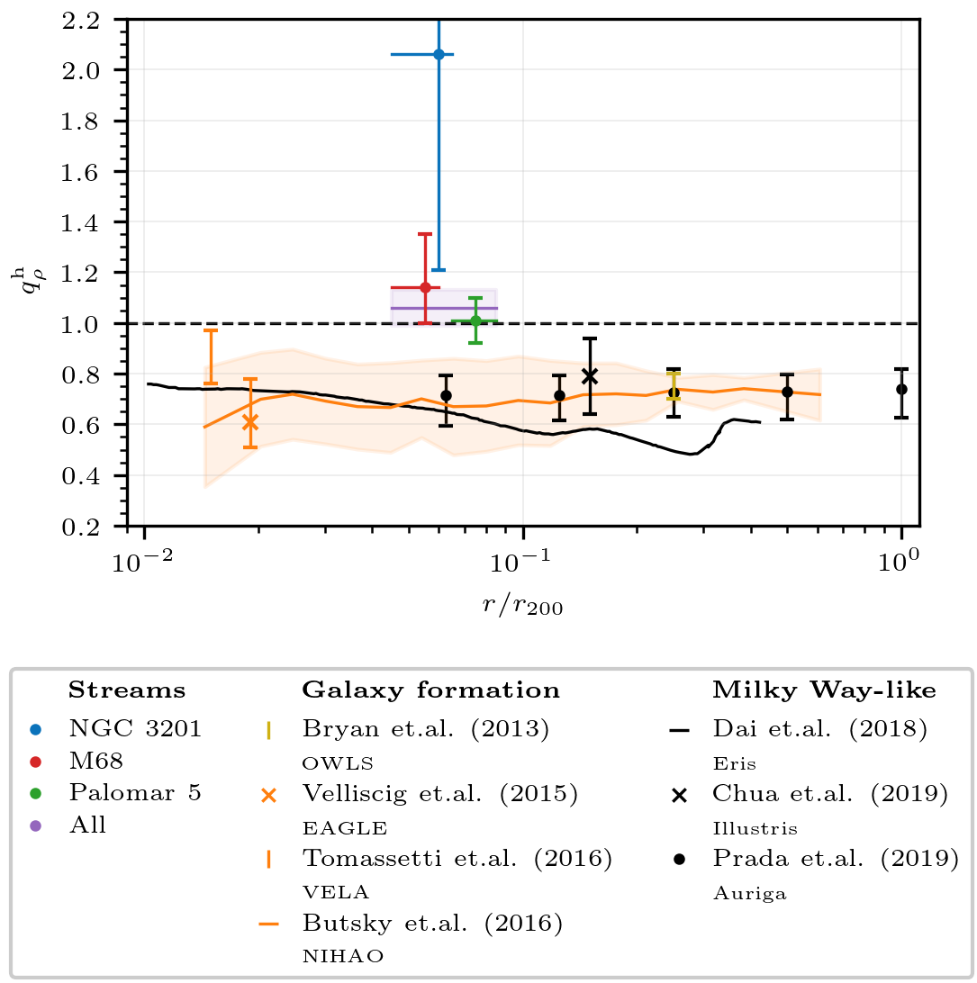
Figure 9: Comparison of our estimates of $q_{\rho}^{\rm h}$ from each of our three streams (red for M68, blue for NGC 3201, green for Palomar 5), and all streams together (purple), to predictions of the halo axis ratio from simulations of galaxy formation. Black dots with error bars and shaded areas are mean values and $1\sigma$ ranges in the halo axis ratios measured in disc galaxy host halos along the axis perpendicular to the disc plane (no dot is shown when the result is given as an interval in the referenced works). The simulation name appears under each reference. The simulated galaxies have $r_{200}\mathrel{\mathchoice{\raise 0.0pt\hbox{\scalebox{0.8}{\raise 0.0pt\hbox{$\displaystyle\sim$}}}}{\raise 0.0pt\hbox{\scalebox{0.8}{\raise 0.0pt\hbox{$\textstyle\sim$}}}}{\raise 0.0pt\hbox{\scalebox{0.8}{\raise 0.0pt\hbox{$\scriptstyle\sim$}}}}{\raise 0.0pt\hbox{\scalebox{0.8}{\raise 0.0pt\hbox{$\scriptscriptstyle\sim$}}}}}[200\,\text{,}\,240]$ kpc. Our stream model results are shown at the mean distance of each stream, with its radial range shown as a horizontal bar, and the whole range indicated by the all streams model as the purple line. The dashed horizontal line marks the spherical shape.

6.4 Influence of the Magellanic Clouds

An important question in relation to the observationally inferred estimates of the shape of the Milky Way dark matter halo, and the comparison to predictions from numerical simulations, is the influence that the Magellanic Clouds may have in distorting this halo shape in their encounter with the Milky Way galaxy. Recent studies have shown that the Magellanic Clouds are in their first orbital passage through their pericentre around the Milky Way galaxy, and that their associated dark matter halo may be as massive as $\mathrel{\mathchoice{\raise 0.0pt\hbox{\scalebox{0.8}{\raise 0.0pt\hbox{$\displaystyle\sim$}}}}{\raise 0.0pt\hbox{\scalebox{0.8}{\raise 0.0pt\hbox{$\textstyle\sim$}}}}{\raise 0.0pt\hbox{\scalebox{0.8}{\raise 0.0pt\hbox{$\scriptstyle\sim$}}}}{\raise 0.0pt\hbox{\scalebox{0.8}{\raise 0.0pt\hbox{$\scriptscriptstyle\sim$}}}}}1/4$ of the Milky Way dark matter halo (see e.g. Erkal et al., 2019; Gardner et al., 2020; Patel et al., 2020). Thus, the merger of the Milky Way with the Magellanic Clouds that is unfolding at present is not so much a "minor merger", but a merger of two galactic systems that are more closely comparable in mass than was thought in the past.

The Milky Way dark matter halo at a distance $r$ from the centre is in a dynamical state governed by the acceleration $g_{\>\!\scalebox{0.65}{MW}}\mathrel{\mathchoice{\raise 0.0pt\hbox{\scalebox{0.8}{\raise 0.0pt\hbox{$\displaystyle\sim$}}}}{\raise 0.0pt\hbox{\scalebox{0.8}{\raise 0.0pt\hbox{$\textstyle\sim$}}}}{\raise 0.0pt\hbox{\scalebox{0.8}{\raise 0.0pt\hbox{$\scriptstyle\sim$}}}}{\raise 0.0pt\hbox{\scalebox{0.8}{\raise 0.0pt\hbox{$\scriptscriptstyle\sim$}}}}}GM_{\scalebox{0.65}{MW}}/r^{2}$, where $M_{\scalebox{0.65}{MW}}$ is the total Milky Way mass within $r$, and is perturbed by the gravitational tide of the Magellanic Cloud system at a distance $d$ from the Milky Way centre. This tidal acceleration is, to first order in $r/d$, $g_{\>\!\scalebox{0.65}{MC}}\mathrel{\mathchoice{\raise 0.0pt\hbox{\scalebox{0.8}{\raise 0.0pt\hbox{$\displaystyle\sim$}}}}{\raise 0.0pt\hbox{\scalebox{0.8}{\raise 0.0pt\hbox{$\textstyle\sim$}}}}{\raise 0.0pt\hbox{\scalebox{0.8}{\raise 0.0pt\hbox{$\scriptstyle\sim$}}}}{\raise 0.0pt\hbox{\scalebox{0.8}{\raise 0.0pt\hbox{$\scriptscriptstyle\sim$}}}}}GM_{\scalebox{0.65}{MC}}\,r/d^{3}$, so the ratio of the two accelerations is:

$$\dfrac{g_{\>\!\scalebox{0.65}{MW}}}{g_{\>\!\scalebox{0.65}{MC}}}=\dfrac{M_{\scalebox{0.65}{MW}}\,d^{3}}{M_{\scalebox{0.65}{MC}}\,r^{3}}~{}.$$ (15)

Our measurements of the Milky Way halo shape are at $r<20\,{\rm kpc}$, and the Galactocentric distance to the Magellanic clouds is $d\simeq 50\,{\rm kpc}$, so we conclude that for $M_{\scalebox{0.65}{MW}}/M_{\scalebox{0.65}{MC}}\simeq 4$, the tidal influence of the LMC is no larger than $\mathrel{\mathchoice{\raise 0.0pt\hbox{\scalebox{0.8}{\raise 0.0pt\hbox{$\displaystyle\sim$}}}}{\raise 0.0pt\hbox{\scalebox{0.8}{\raise 0.0pt\hbox{$\textstyle\sim$}}}}{\raise 0.0pt\hbox{\scalebox{0.8}{\raise 0.0pt\hbox{$\scriptstyle\sim$}}}}{\raise 0.0pt\hbox{\scalebox{0.8}{\raise 0.0pt\hbox{$\scriptscriptstyle\sim$}}}}}$ 2 per cent of the usual acceleration in the Milky Way for the stellar streams we study. In addition, the distance of the streams to the LMC is always greater than about 40 kpc, with the closest approximation being approximately 45 kpc for NGC 3201, 37 kpc for M68, and 40 kpc for Palomar 5. We therefore conclude that the Magellanic Clouds should not be affecting our conclusions, although it is certainly important to include their effect for studies going to larger radius or seeking higher accuracy in the halo shape determination.

6.5 Consequences for the Milky Way halo dynamical equilibrium state

A spherical dark matter halo surrounding the Milky Way galaxy in the presence of the disk cannot have an isotropic velocity dispersion. In order to be supported in the oblate gravitational potential that results from the combined mass distribution of the halo and disk, the velocity dispersion must be higher in the vertical direction (perpendicular to the disk) compared to the two directions in the disk plane. This is a consequence of the tensor virial theorem and the Vlasov equations of dynamical equilibrium (Binney & Tremaine, 2008). The velocity anisotropy is important if the halo is substantially less oblate than the isopotential surfaces, in the region where the disk mass is comparable to the halo one. We have found the Milky Way halo to be close to spherical (or slightly prolate) in the radial interval of $10$ to $20$ kpc, which suggests the presence of this anisotropic velocity dispersion of the dark matter in the Milky Way.

This anisotropy in the velocity dispersion will need to be further analyzed in future work to quantify its presence, but if real, it would have to originate from an originally prolate halo with a long axis perpendicular to the disk formed in the assembly process of the Milky Way halo. In addition, interactions of the dark matter particles with the baryonic components of the Milky Way (in particular the bulge density cusp and a rotating bar, which result in random scatterings of distant particles moving through the central galaxy region) should tend to isotropize the dark matter velocity dispersion and thereby increase the halo oblateness. This probably requires a more strongly prolate shape of the original Milky Way halo shape to reach a nearly spherical configuration in the present Galaxy at radii in 10 to 20 kpc range.

Future studies will need to address this issue of the required initial anisotropic configuration of the halo to support the halo shape at the radii where the baryonic contribution to the potential is important.

7 Conclusion

Stellar streams provide us with a powerful methodology to measure the gravitational potential of the Milky Way and to infer the distribution of mass which, when taking into account the contribution of visible baryonic matter, can give us indications on the distribution of dark matter. One of the most interesting constraints we can derive is the departure from sphericity of the dark matter halo, and test if the halo is oblate or prolate with respect to the disc at different radii. The distribution of the halo axis ratio at different radii can be compared with predictions of galaxy formation from cosmological simulations. In the past, the mass distribution could be constrained only from the kinematic distributions of various tracers in the Milky Way using assumptions of dynamical equilibrium, but stellar streams from tidally disrupted systems allow an indirect measurement of accelerations, because the stream trajectory indicates the orbit of the tidally truncated system, except for small deviations that can be modelled and corrected (see e.g. Küpper et al., 2015; Bovy et al., 2016; Malhan & Ibata, 2019).

We have used three streams to model the Milky Way potential in this paper, arising from the tidal stripping of globular clusters NGC 3201, M68, and Palomar 5. We expect that in the future, the large number of other streams being discovered will be used in conjunction to obtain the best constraints on the Milky Way potential, but this paper is our initial attempt to obtain such constraints based on three streams that appear particularly interesting at this time due to their proximity and available members in the Gaia catalogue. After selecting a list of members of these streams with our maximum likelihood method, we have fitted a model of the Galactic potential based on 5 free parameters of an axisymmetric dark matter halo (mass, inner and outer slope, core radius, and axis ratio), while adding other free parameters for the baryonic components that are subject to various prior observational constraints (the Sun’s position and velocity, the rotation curve in the radial range from 5 to 25 kpc, other star kinematics, and velocities of distant Milky Way satellites).

To show how the constraints arise from each stream, our results have been presented as parameterized models fitted to each stream individually, and to all three stream together. Our interest focuses mainly on the dark matter halo oblateness, to use this as a test of dark matter theories that can predict the distribution of the axis ratio. We find that while the NGC 3201 stream is not very sensitive to this axis ratio, the Palomar 5 stream gives a strong constraint of $q_{\rho}^{\rm h}=1.01\pm 0.09$, and the M68 stream yields $q_{\rho}^{\rm h}=1.14^{+0.21}_{-0.14}$, owing to favorable trajectories of these streams that are sensitive to the acceleration differences introduced by the halo oblateness. The parameter degeneracy is reduced by the priors from other available data on the rotation curve and vertical velocity dispersion of the disc. In the case of the M68 model, the oblateness parameter is correlated mainly with the disc mass. A more massive disc is preferred, but the final constraint on $q_{\rho}^{\rm h}$ is compatible with the other streams. Our combined result on the axis ratio from the three streams is $q_{\rho}^{\rm h}=1.06\pm 0.06$, consistent with a spherical halo with a statistical preference for a slightly prolate halo. Our model assumes a halo axis ratio that is independent of radius, and these constraints are to be understood as applying near the radius that is probed by the streams, at $r\mathrel{\mathchoice{\raise 0.0pt\hbox{\scalebox{0.8}{\raise 0.0pt\hbox{$\displaystyle\sim$}}}}{\raise 0.0pt\hbox{\scalebox{0.8}{\raise 0.0pt\hbox{$\textstyle\sim$}}}}{\raise 0.0pt\hbox{\scalebox{0.8}{\raise 0.0pt\hbox{$\scriptstyle\sim$}}}}{\raise 0.0pt\hbox{\scalebox{0.8}{\raise 0.0pt\hbox{$\scriptscriptstyle\sim$}}}}}10$ to $20\,{\rm kpc}$. This result agrees with previous studies using different observational data and fitting methodology.

Our best fit model also demands a very shallow density profile for the dark matter halo, with inner slope $\alpha$ close to zero and a large core radius of $\mathrel{\mathchoice{\raise 0.0pt\hbox{\scalebox{0.8}{\raise 0.0pt\hbox{$\displaystyle\sim$}}}}{\raise 0.0pt\hbox{\scalebox{0.8}{\raise 0.0pt\hbox{$\textstyle\sim$}}}}{\raise 0.0pt\hbox{\scalebox{0.8}{\raise 0.0pt\hbox{$\scriptstyle\sim$}}}}{\raise 0.0pt\hbox{\scalebox{0.8}{\raise 0.0pt\hbox{$\scriptscriptstyle\sim$}}}}}15\,{\rm kpc}$. The flatness of the density profile in the inner region is also interesting to test the way that the formation of the disc and bar and the presence of gas inflows and outflows over the history of the Milky Way may have flattened the central parts of dark matter halo. Nevertheless, the inner dark matter distribution is probably degenerate with the baryonic mass component in the inner disc, bar and bulge. Our model simply includes an exponential disc with no inner cutoff and a bulge with only one free parameter (the mass), and a more careful treatment of the mass distribution at $r\mathrel{\mathchoice{\raise 0.0pt\hbox{\scalebox{0.8}{\raise 0.0pt\hbox{$\displaystyle\lesssim$}}}}{\raise 0.0pt\hbox{\scalebox{0.8}{\raise 0.0pt\hbox{$\textstyle\lesssim$}}}}{\raise 0.0pt\hbox{\scalebox{0.8}{\raise 0.0pt\hbox{$\scriptstyle\lesssim$}}}}{\raise 0.0pt\hbox{\scalebox{0.8}{\raise 0.0pt\hbox{$\scriptscriptstyle\lesssim$}}}}}5\,{\rm kpc}$ is needed to more rigorously test constraints on the inner dark matter profile. Our model constraints on the outer dark matter density slope and total mass $M_{\rm 200}$ are also mainly dependent on the constraints from external satellite kinematic data we use.

The Milky Way dark matter halo density model should be greatly improved in the future by including the large number of stellar streams that are being discovered with a wide range of orbits in the Milky Way halo. Some of the most interesting cases are the streams generated by globular clusters NGC 5466 and M5, with similar characteristics and locations as the streams used in this study. A greater variety of models and parameters should also be included, and the impact of the gravitational perturbation by the Magellanic Clouds and other massive satellites should be incorporated as we probe the halo density profile and oblateness at larger radius and/or with greater accuracy than in this study.

At present, we can already say that most of the cosmological simulations that have been analyzed in relation to the question of the oblateness of galactic halos seem to predict oblate halos, with axis ratio lower than the 2-$\sigma$ lower limit from our study. This may be a possible discrepancy with Cold Dark Matter theories, indicating that either the dark matter has some new property that tends to make halos more spherical in the inner parts, or that the Milky Way is a peculiar galaxy with its halo long axis perpendicular to the disc, while the results of simulations indicate that most galaxies should have the oblate halos. We have pointed out that a spherical halo, in the presence of the gravitational potential of the disc, actually needs to maintain an anisotropic velocity dispersion, with greater dispersion along the vertical axis compared to the horizontal ones, to maintain its spherical shape in equilibrium, and this becomes important at the radius where the disc and halo contributions to the gravitational potential are comparable, at $r\mathrel{\mathchoice{\raise 0.0pt\hbox{\scalebox{0.8}{\raise 0.0pt\hbox{$\displaystyle\sim$}}}}{\raise 0.0pt\hbox{\scalebox{0.8}{\raise 0.0pt\hbox{$\textstyle\sim$}}}}{\raise 0.0pt\hbox{\scalebox{0.8}{\raise 0.0pt\hbox{$\scriptstyle\sim$}}}}{\raise 0.0pt\hbox{\scalebox{0.8}{\raise 0.0pt\hbox{$\scriptscriptstyle\sim$}}}}}10\,{\rm kpc}$. This suggests that it is difficult to avoid having an oblate dark matter halo in the inner regions of the galaxy, if random scatterings (caused, for example, by a rotating bar or the central density cusp and black hole in the bulge) tend to isotropize the orbital motions of the dark matter. Future studies, using improved data from streams and stellar kinematic constraints, and more general models for the gravitational potential, will hopefully clarify these questions on the Milky Way dark matter halo.

Data Availability

The data on which this article is based are available in the article itself and in the references included therein.

Appendix A Observed sections of NGC 3201 and M68 streams

The section of the NGC 3201 used to constrain the Galactic potential is populated by 54 stars selected in PM21 within the limits of $65<\alpha<120$ deg and located between about 3 and 4 kpc from the Sun. In the top panel of Figure 10 we show the selected stars in blue, and in black, the foreground passing the pre-section cut defined in Section 3.3 of PM19 with a threshold $P_{\scaleto{\rm REG}{3.5pt}}=0.5$ ${\rm yr}^{3}\,{\rm deg}^{-2}\,{\rm pc}^{-1}\,{\rm mas}^{-3}$. We also mark the boundaries of our selection with vertical dashed lines.

In summary, the pre-section removes stars with a parallax $\pi>1/0.3$ mas and selects the stars compatible with the HR-diagram of NGC 3201 using the method described in Section 3.3 of PM21. It also selects stars with proper motions $\mathrel{\mathchoice{\raise 0.0pt\hbox{\scalebox{0.8}{\raise 0.0pt\hbox{$\displaystyle\gtrsim$}}}}{\raise 0.0pt\hbox{\scalebox{0.8}{\raise 0.0pt\hbox{$\textstyle\gtrsim$}}}}{\raise 0.0pt\hbox{\scalebox{0.8}{\raise 0.0pt\hbox{$\scriptstyle\gtrsim$}}}}{\raise 0.0pt\hbox{\scalebox{0.8}{\raise 0.0pt\hbox{$\scriptscriptstyle\gtrsim$}}}}}10$ mas yr^-1 in a region around the orbit of the cluster wide enough not to eliminate potential candidate stars. For example, we can see how stars located far from the stream, at $\alpha\mathrel{\mathchoice{\raise 0.0pt\hbox{\scalebox{0.8}{\raise 0.0pt\hbox{$\displaystyle\sim$}}}}{\raise 0.0pt\hbox{\scalebox{0.8}{\raise 0.0pt\hbox{$\textstyle\sim$}}}}{\raise 0.0pt\hbox{\scalebox{0.8}{\raise 0.0pt\hbox{$\scriptstyle\sim$}}}}{\raise 0.0pt\hbox{\scalebox{0.8}{\raise 0.0pt\hbox{$\scriptscriptstyle\sim$}}}}}80$ and $\delta\mathrel{\mathchoice{\raise 0.0pt\hbox{\scalebox{0.8}{\raise 0.0pt\hbox{$\displaystyle\sim$}}}}{\raise 0.0pt\hbox{\scalebox{0.8}{\raise 0.0pt\hbox{$\textstyle\sim$}}}}{\raise 0.0pt\hbox{\scalebox{0.8}{\raise 0.0pt\hbox{$\scriptstyle\sim$}}}}{\raise 0.0pt\hbox{\scalebox{0.8}{\raise 0.0pt\hbox{$\scriptscriptstyle\sim$}}}}}6$ deg pass through these pre-selection cuts. The pre-selection is more restrictive in the colour and magnitude space, where we exclude stars with large observational uncertainties. This does not alter the stream track, but enhances the star overdensity in sky coordinates.

Within the defined limits, the stream can be seen without ambiguity due to its high population and low number of foreground stars (in Section 3.1 of PM21 we show how the expected number of foreground stars along the overdensity is between 4 and 8). The final selection consists of stars that intersect a density model of the stream. We compute the intersection using the method described in Section 4.3 of PM19. The density model of the stream is approximately a cylinder that follows the overdensity of stars in phase-space. Its diameter is determined by a selection threshold $\chi_{\rm sel}$ given in Section 3.4 of PM21, optimised to include stars along the overdensity but exclude the observed foreground. Some stars located along the stream have not been included in the final selection. This is due to their large proper motion uncertainties compared to the selected stars. Their exclusion from our sample does not change the track of the stream, and therefore the constraints on the Galactic potential obtained with this selection.

The stream of M68 is shown in red in the bottom panel of Figure 10. We select 98 stars from the final selection of PM19. We also plot the foreground stars which pass through a similar pre-selection cut as described above. As in the previous case, the pre-selection cut does not remove many stream stars using their position in phase-space. We note that some stars located at about 25 deg perpendicular to the orbit pass through these cuts. The most restrictive cuts are applied in colour and magnitude space, as the loss of faint stars with large observational uncertainties does not alter the stream track.

The stream is clearly visible when it is close to the Sun, at about 5 kpc, in the interval $190<\alpha<260$ deg. We have excluded the region with $\delta<-8$ deg because the stream is located at about 10 kpc from the Sun and beyond, and appears to be projected closer to the disc. In this region, there is a high level of foreground star contamination. For similar reasons, no stars have been selected for $\alpha>275$ deg.

There are several stars located around the stream, especially above our selection, between $190<\alpha<240$ deg. These stars form a diffuse envelope or cocoon, similar to the presented by other streams such as GD-1 (Malhan et al., 2019) or Jhelum (Woudenberg et al., 2023). These stars can be separated from the stream because their proper motions are significantly larger, and they are aligned in proper motion space following a different orbit clearly distinguishable from the main stream. This orbit cannot be followed by either the cluster or its stream for any reasonable Galactic potential. This may be a consequence of the stellar envelope being closer to the Sun than the stream. A detailed analysis of the structure of the stream and its diffuse envelope will be realised when radial velocities and better measurements are available from future releases of the Gaia catalogue.

Similarly to the previous case, several stars along the stream have not been selected due to their comparatively large proper motion uncertainties. It is likely that the majority of these stars belong to the stream. In Section 4.3 of PM19 we showed that we expect only 1 or 2 foreground stars along the stream overdensity within the defined limits. Excluding these stars does not change the stream track, and therefore the constraints on the potential obtained by fitting this star selection.

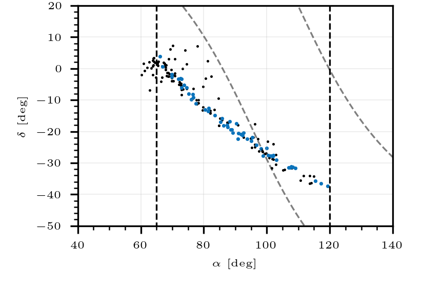
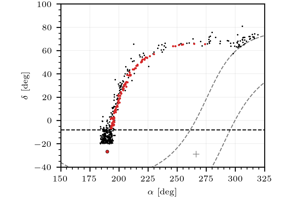
Figure 10: Sky map in equatorial coordinates of a sample of pre-selected stars (black dots) and the final selection of stream stars (coloured dots) used to constrain the potential of the Milky Way. Grey dashed lines indicate a Galactic latitude $b=\pm 15$ deg and the grey cross the Galactic centre. Top panel: Blue dots mark the selected NGC 3201 stream stars. The black dashed lines at $\alpha=65$ and $120$ deg mark the limits of the selection zone. Bottom panel: Red dots mark the selected M68 stream stars. The black dashed line at $\delta=-8$ deg marks the boundary of the selection zone. The large red dot marks the current position of the cluster.

Appendix B Final selection of Palomar 5 tidal stream members

To select the stars most likely to belong to the Palomar 5 stellar stream, we use the method described in PM19. First, we apply the pre-selection cuts defined in Section 3.3 of PM19 to reduce the number of foreground stars surrounding the stream. These cuts basically select stars near the orbit of the cluster, in a $\pm 20$ Myr section of the orbit from the cluster centre. They also remove the stars belonging to the globular cluster Palomar 5 and M5 to avoid detecting overdensities that do not correspond to streams. After the pre-selection, we obtain 320 302 GDR2 sources. We apply the same pre-selection to a simulation of the GDR2 catalogue, the 18th version of the Gaia Object Generator (GOG18, Luri et al., 2014) obtaining 450 622 sources. This 30 per cent difference can be explained by imperfect modeling of the stellar halo in GOG18, by inaccuracies in the simulation of GDR2 uncertainties, or because GDR2 does not include all sources with $G\>\!\text{-band}$ magnitude $G<21$ mag in low exposure areas.

We apply the maximum likelihood method explained in Section 2 of PM19 to compute the best-fitting parameters of the stream model, as well as the statistic $\Lambda$ indicating the confidence level with which the stream is detected. When $\Lambda>6.6$, the existence of the stream is confirmed at the 99 per cent confidence level, as opposed to the null hypothesis that no stream is present in the pre-selection. We detect the stellar stream with $\Lambda=14.44$, which implies a high statistical significance of the detection. We compute an accurate phase-space density model of the stream using the best-fitting configuration of the free parameters. We select the stars with the largest intersection with this model. We define a threshold for the value of the intersection $\chi_{\rm sel}$, and choose stars with $\chi_{\rm sel}>4.6$ yr³ deg^-2 pc^-1 mas^-3. We obtain 229 stars from the GRD2 catalogue compatible with the phase-space density model of the stream. For the chosen threshold, we select no stars from the GOG18 catalogue. This minimizes the number of expected foreground stars erroneously selected as Palomar 5 stream members.

Finally, we only select stars that are compatible in colour and magnitude with the H-R diagram of Palomar 5. We follow the procedure described in Appendix D of PM19 and include the correction for dust extinction described in Appendix B of PM21. In Table 3, we list the 126 star candidates belonging to the Palomar 5 tidal stream selected from the GDR2 catalogue. None of these stars have radial velocity measured by Gaia, but 15 of them match stars with radial velocity measured by Ibata et al. (2017). We list their values in Table 4.

Table 3: Stars compatible with the best-fitting phase-space density model of the tidal stream of Palomar 5 and its H-R diagram from GDR2 after dust extinction correction.

N	source_id	$\pi$	$\delta$	$\alpha$	$\mu_{\delta}$	$\mu_{\alpha*}$	$G_{\rm BP}\!-\!G_{\rm RP}$	$G$	$\chi_{\rm sel}$
		(mas)	(deg)	(deg)	(mas yr-1)	(mas yr-1)	(mag)	(mag)	( yr3 deg-2 pc-1 mas-3 )
1	6327240546525053824	$-0.1349$	$-8.1333$	$222.5158$	$-2.4483$	$-2.4054$	$1.0417$	$17.5562$	$5.9454\text{E}\>\!\>\!\scalebox{0.75}[1.0]{$+$}\>\!00$
2	6327454916932476800	$-0.0426$	$-7.9192$	$222.6962$	$-2.4659$	$-2.3107$	$1.0067$	$17.8507$	$8.2674\text{E}\>\!\>\!\scalebox{0.75}[1.0]{$+$}\>\!00$
3	6333632175119962368	$0.1395$	$-6.8635$	$223.3798$	$-2.4777$	$-2.6496$	$0.9335$	$19.4622$	$5.6500\text{E}\>\!\>\!\scalebox{0.75}[1.0]{$+$}\>\!00$
4	6333638840909351808	$0.3333$	$-6.7025$	$223.7207$	$-2.6044$	$-2.5148$	$1.0312$	$17.8252$	$1.3563\text{E}\>\!\>\!\scalebox{0.75}[1.0]{$+$}\>\!01$
5	6334133694157081856	$0.0026$	$-5.8463$	$223.8334$	$-2.3926$	$-2.7662$	$1.1181$	$17.5348$	$1.2756\text{E}\>\!\>\!\scalebox{0.75}[1.0]{$+$}\>\!01$
6	6337139376694381440	$-0.1242$	$-5.6805$	$223.9155$	$-2.4263$	$-2.7577$	$0.9366$	$17.4458$	$4.8662\text{E}\>\!\>\!\scalebox{0.75}[1.0]{$+$}\>\!00$
7	6334151110248964224	$0.0510$	$-5.6672$	$224.4260$	$-3.1251$	$-2.0798$	$1.0594$	$18.7005$	$1.4053\text{E}\>\!\>\!\scalebox{0.75}[1.0]{$+$}\>\!01$
8	6334300162794237184	$0.5529$	$-5.0987$	$224.7233$	$-2.7727$	$-1.9366$	$1.0851$	$19.0335$	$6.7220\text{E}\>\!\>\!\scalebox{0.75}[1.0]{$+$}\>\!00$
9	6338851453738047488	$0.1009$	$-4.2145$	$224.9720$	$-2.6403$	$-2.1383$	$1.0813$	$18.4176$	$9.9368\text{E}\>\!\>\!\scalebox{0.75}[1.0]{$+$}\>\!00$
10	6334298169929419392	$0.1771$	$-5.0869$	$224.9823$	$-2.4609$	$-2.7599$	$1.0623$	$18.1751$	$6.6524\text{E}\>\!\>\!\scalebox{0.75}[1.0]{$+$}\>\!00$
11	6338874990158885376	$0.1463$	$-4.1744$	$225.0625$	$-2.7762$	$-2.3852$	$1.0872$	$17.7758$	$3.4422\text{E}\>\!\>\!\scalebox{0.75}[1.0]{$+$}\>\!01$
12	6338879564298848640	$-0.0324$	$-4.0963$	$225.3011$	$-2.4097$	$-1.2524$	$1.1311$	$18.9155$	$4.8295\text{E}\>\!\>\!\scalebox{0.75}[1.0]{$+$}\>\!00$
13	6338859562636251904	$0.2195$	$-4.2534$	$225.3258$	$-2.5176$	$-1.7848$	$1.1024$	$18.0456$	$3.3353\text{E}\>\!\>\!\scalebox{0.75}[1.0]{$+$}\>\!01$
14	6338880487717174528	$0.0521$	$-4.0583$	$225.4573$	$-2.3537$	$-3.1365$	$1.1220$	$17.6939$	$1.0366\text{E}\>\!\>\!\scalebox{0.75}[1.0]{$+$}\>\!01$
15	6338869149003524224	$-0.0925$	$-4.0479$	$225.5377$	$-3.0576$	$-2.0272$	$1.0265$	$19.2443$	$2.1193\text{E}\>\!\>\!\scalebox{0.75}[1.0]{$+$}\>\!01$
16	6339016002525065472	$0.0639$	$-3.5563$	$225.7535$	$-2.3171$	$-3.4270$	$1.1729$	$19.0526$	$5.8216\text{E}\>\!\>\!\scalebox{0.75}[1.0]{$+$}\>\!00$
17	6338987758819995776	$-0.1428$	$-3.6964$	$225.7778$	$-2.4940$	$-2.3050$	$1.1700$	$18.7510$	$8.4701\text{E}\>\!\>\!\scalebox{0.75}[1.0]{$+$}\>\!01$
18	6339017823591238400	$0.0527$	$-3.5147$	$225.8524$	$-2.6521$	$-3.2807$	$1.3766$	$20.0483$	$7.4983\text{E}\>\!\>\!\scalebox{0.75}[1.0]{$+$}\>\!00$
19	6339403580374320896	$0.2071$	$-3.2162$	$226.1388$	$-2.8443$	$-2.8832$	$1.1255$	$19.7879$	$5.9449\text{E}\>\!\>\!\scalebox{0.75}[1.0]{$+$}\>\!00$
20	6339405195282047232	$0.3347$	$-3.1899$	$226.1702$	$-1.9488$	$-2.9943$	$1.1956$	$17.8007$	$7.7164\text{E}\>\!\>\!\scalebox{0.75}[1.0]{$+$}\>\!00$
21	6339486112465206528	$0.2516$	$-2.9349$	$226.3743$	$-2.9628$	$-2.5859$	$1.1431$	$18.1520$	$2.8470\text{E}\>\!\>\!\scalebox{0.75}[1.0]{$+$}\>\!01$
22	6339492091059869696	$0.1419$	$-2.7626$	$226.4066$	$-1.7571$	$-2.2625$	$1.0337$	$19.6753$	$5.6089\text{E}\>\!\>\!\scalebox{0.75}[1.0]{$+$}\>\!00$
23	6339498589346000768	$-0.0427$	$-2.7155$	$226.4922$	$-2.9333$	$-2.4861$	$0.5547$	$17.4368$	$8.3411\text{E}\>\!\>\!\scalebox{0.75}[1.0]{$+$}\>\!00$
24	6339607745939180928	$0.2627$	$-2.2781$	$226.9747$	$-1.9119$	$-2.3462$	$0.9989$	$19.5513$	$1.8167\text{E}\>\!\>\!\scalebox{0.75}[1.0]{$+$}\>\!01$
25	6339642724153085056	$-0.4911$	$-1.9832$	$227.2439$	$-2.5559$	$-3.2388$	$0.7922$	$19.9143$	$5.0767\text{E}\>\!\>\!\scalebox{0.75}[1.0]{$+$}\>\!00$
26	6339639666136263040	$-0.2089$	$-2.0898$	$227.2613$	$-2.4832$	$-2.1312$	$0.8322$	$17.1603$	$1.3918\text{E}\>\!\>\!\scalebox{0.75}[1.0]{$+$}\>\!02$
27	4418107238191732352	$-0.0317$	$-1.9491$	$227.3442$	$-3.2361$	$-2.4779$	$0.7086$	$20.1749$	$5.3026\text{E}\>\!\>\!\scalebox{0.75}[1.0]{$+$}\>\!00$
28	4418156892309715456	$0.0184$	$-1.5275$	$227.7144$	$-2.7810$	$-2.9716$	$0.9151$	$18.6426$	$1.2555\text{E}\>\!\>\!\scalebox{0.75}[1.0]{$+$}\>\!01$
29	4418142117622280192	$-0.2247$	$-1.6319$	$227.7547$	$-2.2909$	$-2.6730$	$0.5875$	$17.3171$	$8.1503\text{E}\>\!\>\!\scalebox{0.75}[1.0]{$+$}\>\!00$
30	4418143968756451968	$0.1305$	$-1.5872$	$227.8667$	$-2.7425$	$-2.7935$	$0.9761$	$19.4101$	$5.1128\text{E}\>\!\>\!\scalebox{0.75}[1.0]{$+$}\>\!00$
31	4418261930029664256	$0.1726$	$-1.2314$	$227.9615$	$-2.4465$	$-2.4811$	$0.8722$	$17.4131$	$3.7794\text{E}\>\!\>\!\scalebox{0.75}[1.0]{$+$}\>\!02$
32	4418265022406118784	$0.1443$	$-1.2007$	$227.9690$	$-2.5811$	$-2.7873$	$1.1245$	$17.1479$	$1.0070\text{E}\>\!\>\!\scalebox{0.75}[1.0]{$+$}\>\!01$
33	4418300339922183040	$-0.2577$	$-0.9056$	$228.2730$	$-1.2246$	$-2.4189$	$1.1503$	$19.2080$	$5.7784\text{E}\>\!\>\!\scalebox{0.75}[1.0]{$+$}\>\!00$
34	4418296800869119488	$-0.0699$	$-0.9458$	$228.3485$	$-2.5452$	$-2.5164$	$1.0382$	$18.2234$	$9.5543\text{E}\>\!\>\!\scalebox{0.75}[1.0]{$+$}\>\!01$
35	4418305219004364416	$0.0308$	$-0.8191$	$228.4767$	$-2.3525$	$-3.1096$	$1.0936$	$18.2519$	$2.0354\text{E}\>\!\>\!\scalebox{0.75}[1.0]{$+$}\>\!01$
36	4418876999410407808	$0.1810$	$-0.5154$	$228.4965$	$-2.6434$	$-2.8694$	$1.0682$	$18.4087$	$5.3204\text{E}\>\!\>\!\scalebox{0.75}[1.0]{$+$}\>\!00$
37	4418292299742718336	$0.2783$	$-0.8791$	$228.5547$	$-3.1739$	$-2.0598$	$1.2035$	$18.9636$	$4.8350\text{E}\>\!\>\!\scalebox{0.75}[1.0]{$+$}\>\!00$
38	4418688536245813888	$0.0397$	$-0.5523$	$228.5716$	$-2.8887$	$-2.5161$	$1.0884$	$17.9491$	$8.2213\text{E}\>\!\>\!\scalebox{0.75}[1.0]{$+$}\>\!00$
39	4418306490314700416	$-0.0735$	$-0.7719$	$228.5788$	$-2.9618$	$-2.6038$	$1.0582$	$18.5771$	$1.1654\text{E}\>\!\>\!\scalebox{0.75}[1.0]{$+$}\>\!01$
40	4418306387235478784	$0.0103$	$-0.7888$	$228.5841$	$-2.9801$	$-2.6432$	$1.1172$	$18.7119$	$1.0503\text{E}\>\!\>\!\scalebox{0.75}[1.0]{$+$}\>\!01$
41	4418306490314700288	$0.0571$	$-0.7728$	$228.5863$	$-2.6047$	$-2.1894$	$1.1371$	$17.5508$	$1.8540\text{E}\>\!\>\!\scalebox{0.75}[1.0]{$+$}\>\!02$
42	4418307899063987584	$0.4335$	$-0.7168$	$228.6229$	$-1.9881$	$-2.0470$	$0.9793$	$19.0673$	$1.4992\text{E}\>\!\>\!\scalebox{0.75}[1.0]{$+$}\>\!01$
43	4418687161856244096	$-0.0988$	$-0.6207$	$228.6410$	$-2.4472$	$-2.8298$	$0.7099$	$17.1817$	$4.8383\text{E}\>\!\>\!\scalebox{0.75}[1.0]{$+$}\>\!00$
44	4418889815592901248	$0.0445$	$-0.2970$	$228.6474$	$-2.2003$	$-2.2111$	$1.0924$	$17.7308$	$1.2297\text{E}\>\!\>\!\scalebox{0.75}[1.0]{$+$}\>\!02$
45	4418683485364220160	$0.4711$	$-0.6612$	$228.6626$	$-2.3617$	$-3.3018$	$1.0654$	$19.4714$	$5.8224\text{E}\>\!\>\!\scalebox{0.75}[1.0]{$+$}\>\!00$
46	4418696404625960448	$-0.5780$	$-0.4148$	$228.8240$	$-2.7140$	$-1.9526$	$0.7559$	$19.6628$	$6.0292\text{E}\>\!\>\!\scalebox{0.75}[1.0]{$+$}\>\!00$
47	4418692040939128832	$0.2891$	$-0.5483$	$228.8315$	$-2.1215$	$-3.1551$	$1.1364$	$19.1036$	$8.0271\text{E}\>\!\>\!\scalebox{0.75}[1.0]{$+$}\>\!00$
48	4418698397490799232	$-0.3326$	$-0.3732$	$228.9090$	$-2.4365$	$-1.7305$	$0.6510$	$20.0514$	$6.3760\text{E}\>\!\>\!\scalebox{0.75}[1.0]{$+$}\>\!00$
49	4418679396555391616	$0.2885$	$-0.5816$	$228.9582$	$-2.5619$	$-2.6261$	$1.1009$	$18.5081$	$5.8196\text{E}\>\!\>\!\scalebox{0.75}[1.0]{$+$}\>\!00$
50	4418723583179057024	$0.1416$	$-0.2626$	$228.9601$	$-2.5273$	$-2.7952$	$1.1119$	$17.4493$	$1.2010\text{E}\>\!\>\!\scalebox{0.75}[1.0]{$+$}\>\!01$
51	4418723583179058944	$-0.0373$	$-0.2577$	$228.9661$	$-2.1354$	$-2.8744$	$1.0769$	$19.5808$	$9.7810\text{E}\>\!\>\!\scalebox{0.75}[1.0]{$+$}\>\!00$
52	4418693724566344192	$0.3241$	$-0.4672$	$229.0063$	$-2.7870$	$-2.5274$	$1.1007$	$18.3871$	$4.6609\text{E}\>\!\>\!\scalebox{0.75}[1.0]{$+$}\>\!00$
53	4418926855391616000	$-0.3033$	$+0.0552$	$229.0700$	$-2.0931$	$-2.7288$	$1.0322$	$19.2253$	$5.8788\text{E}\>\!\>\!\scalebox{0.75}[1.0]{$+$}\>\!00$
54	4418724923208864128	$0.3599$	$-0.2139$	$229.0981$	$-3.3158$	$-2.1848$	$0.9962$	$19.1438$	$5.1160\text{E}\>\!\>\!\scalebox{0.75}[1.0]{$+$}\>\!00$
55	4418734165978521728	$-0.0129$	$-0.0736$	$229.1446$	$-2.4978$	$-2.5807$	$0.4412$	$17.4019$	$5.0599\text{E}\>\!\>\!\scalebox{0.75}[1.0]{$+$}\>\!01$
56	4418727225312005504	$0.1660$	$-0.2543$	$229.1711$	$-2.4135$	$-2.2349$	$1.0770$	$18.4655$	$2.0530\text{E}\>\!\>\!\scalebox{0.75}[1.0]{$+$}\>\!01$
57	4418726404973230080	$0.1299$	$-0.2695$	$229.2028$	$-2.3950$	$-2.1456$	$0.8950$	$17.5034$	$7.0368\text{E}\>\!\>\!\scalebox{0.75}[1.0]{$+$}\>\!01$
58	4419023234457620352	$-0.0293$	$+0.2043$	$229.2407$	$-2.4698$	$-2.3608$	$1.0275$	$17.9991$	$1.4207\text{E}\>\!\>\!\scalebox{0.75}[1.0]{$+$}\>\!02$
59	4419073575769649664	$0.5628$	$+0.5239$	$229.3062$	$-1.9015$	$-2.2912$	$1.0387$	$18.1476$	$7.4501\text{E}\>\!\>\!\scalebox{0.75}[1.0]{$+$}\>\!00$
60	4419026842229420800	$-0.1750$	$+0.2297$	$229.3883$	$-2.7700$	$-2.0247$	$1.1586$	$18.8187$	$1.6267\text{E}\>\!\>\!\scalebox{0.75}[1.0]{$+$}\>\!01$
61	4419052405874782592	$0.2759$	$+0.3638$	$229.5968$	$-1.8983$	$-2.9869$	$1.1136$	$18.5392$	$4.7960\text{E}\>\!\>\!\scalebox{0.75}[1.0]{$+$}\>\!00$
62	4419078145614843776	$0.4212$	$+0.6351$	$229.6086$	$-2.3773$	$-2.0128$	$1.1781$	$19.0422$	$1.5265\text{E}\>\!\>\!\scalebox{0.75}[1.0]{$+$}\>\!01$
63	4419068108275272448	$-0.2572$	$+0.6591$	$229.7104$	$-1.4688$	$-2.4685$	$0.9486$	$19.7550$	$6.3516\text{E}\>\!\>\!\scalebox{0.75}[1.0]{$+$}\>\!00$

Table 3: - continued

N	source_id	$\pi$	$\delta$	$\alpha$	$\mu_{\delta}$	$\mu_{\alpha*}$	$G_{\rm BP}\!-\!G_{\rm RP}$	$G$	$\chi_{\rm sel}$
		(mas)	(deg)	(deg)	(mas yr-1)	(mas yr-1)	(mag)	(mag)	( yr3 deg-2 pc-1 mas-3 )
64	4418864767344458112	$-0.0649$	$+0.3228$	$229.7453$	$-2.1466$	$-2.5965$	$1.1113$	$17.9590$	$7.6772\text{E}\>\!\>\!\scalebox{0.75}[1.0]{$+$}\>\!00$
65	4420584403529433728	$0.1415$	$+0.8509$	$229.8402$	$-2.4470$	$-1.9695$	$1.0419$	$18.6502$	$2.9890\text{E}\>\!\>\!\scalebox{0.75}[1.0]{$+$}\>\!01$
66	4420577943898627968	$-0.5387$	$+0.8701$	$230.0352$	$-2.1109$	$-2.9124$	$0.9411$	$19.3734$	$5.3310\text{E}\>\!\>\!\scalebox{0.75}[1.0]{$+$}\>\!00$
67	4420385323205469568	$-0.2093$	$+0.7329$	$230.1499$	$-2.6252$	$-2.1064$	$0.9883$	$18.7577$	$5.4691\text{E}\>\!\>\!\scalebox{0.75}[1.0]{$+$}\>\!00$
68	4420607768151633408	$-0.1165$	$+1.1328$	$230.2065$	$-2.3018$	$-2.7923$	$1.0686$	$17.8563$	$2.3135\text{E}\>\!\>\!\scalebox{0.75}[1.0]{$+$}\>\!01$
69	4420603301385612928	$-0.3072$	$+1.0489$	$230.3098$	$-2.7339$	$-2.0564$	$1.0515$	$18.1806$	$2.5285\text{E}\>\!\>\!\scalebox{0.75}[1.0]{$+$}\>\!01$
70	4420616289367861760	$0.1482$	$+1.2596$	$230.4004$	$-2.1897$	$-2.6394$	$1.1677$	$18.6286$	$5.1850\text{E}\>\!\>\!\scalebox{0.75}[1.0]{$+$}\>\!01$
71	4420608562721387776	$0.2343$	$+1.0585$	$230.4380$	$-2.4493$	$-2.2273$	$1.0231$	$18.2679$	$5.9114\text{E}\>\!\>\!\scalebox{0.75}[1.0]{$+$}\>\!01$
72	4420616048849698304	$0.1699$	$+1.2814$	$230.4905$	$-2.0212$	$-1.9596$	$1.0675$	$18.3503$	$1.0720\text{E}\>\!\>\!\scalebox{0.75}[1.0]{$+$}\>\!02$
73	4420708888861661440	$-0.3825$	$+1.3479$	$230.6310$	$-1.9221$	$-2.4611$	$0.9986$	$18.0155$	$2.2752\text{E}\>\!\>\!\scalebox{0.75}[1.0]{$+$}\>\!01$
74	4420717139494655360	$-0.3145$	$+1.4909$	$230.9006$	$-2.8521$	$-2.1866$	$1.0547$	$17.9769$	$8.1542\text{E}\>\!\>\!\scalebox{0.75}[1.0]{$+$}\>\!00$
75	4420528568955338112	$0.3247$	$+1.4158$	$230.9018$	$-1.9665$	$-3.1172$	$0.9347$	$18.5703$	$1.3916\text{E}\>\!\>\!\scalebox{0.75}[1.0]{$+$}\>\!01$
76	4420553479766045824	$0.1958$	$+1.5626$	$231.0663$	$-1.8110$	$-3.3450$	$0.9903$	$19.1601$	$1.2707\text{E}\>\!\>\!\scalebox{0.75}[1.0]{$+$}\>\!01$
77	4420744283688076672	$0.3469$	$+1.6499$	$231.0725$	$-2.8218$	$-1.8201$	$1.0634$	$18.6081$	$1.0371\text{E}\>\!\>\!\scalebox{0.75}[1.0]{$+$}\>\!01$
78	4420749364634207104	$0.4852$	$+1.6694$	$231.1743$	$-2.4018$	$-3.7009$	$1.2444$	$19.8641$	$5.1075\text{E}\>\!\>\!\scalebox{0.75}[1.0]{$+$}\>\!00$
79	4421127944526566272	$-0.2777$	$+1.8523$	$231.3147$	$-3.3017$	$-2.4256$	$0.8227$	$19.4204$	$5.1616\text{E}\>\!\>\!\scalebox{0.75}[1.0]{$+$}\>\!00$
80	4421128077670137472	$-0.3001$	$+1.8510$	$231.3650$	$-2.1888$	$-3.1238$	$1.0839$	$19.0124$	$6.0021\text{E}\>\!\>\!\scalebox{0.75}[1.0]{$+$}\>\!00$
81	4420939958103532416	$0.2914$	$+1.8132$	$231.3706$	$-2.4673$	$-1.3992$	$1.0720$	$18.7013$	$4.9887\text{E}\>\!\>\!\scalebox{0.75}[1.0]{$+$}\>\!00$
82	4420942432004721408	$-0.5258$	$+1.9198$	$231.5243$	$-1.6142$	$-2.4104$	$0.9329$	$18.6265$	$2.0817\text{E}\>\!\>\!\scalebox{0.75}[1.0]{$+$}\>\!01$
83	4420974111684168320	$0.7073$	$+2.0716$	$231.8210$	$-2.9927$	$-2.4544$	$1.0667$	$19.6251$	$5.2512\text{E}\>\!\>\!\scalebox{0.75}[1.0]{$+$}\>\!00$
84	4420970057233967360	$-0.0405$	$+2.0212$	$231.8757$	$-2.6548$	$-2.9159$	$1.0609$	$18.2706$	$5.5142\text{E}\>\!\>\!\scalebox{0.75}[1.0]{$+$}\>\!00$
85	4420973256984758912	$0.3024$	$+2.1114$	$231.9175$	$-3.2737$	$-1.8754$	$1.1691$	$19.7097$	$5.4066\text{E}\>\!\>\!\scalebox{0.75}[1.0]{$+$}\>\!00$
86	4420985003720258688	$0.1753$	$+2.2946$	$232.0258$	$-1.5876$	$-3.0622$	$0.8244$	$20.1691$	$5.0991\text{E}\>\!\>\!\scalebox{0.75}[1.0]{$+$}\>\!00$
87	4420985553476080768	$0.1695$	$+2.3329$	$232.0740$	$-2.3067$	$-2.7102$	$0.6363$	$19.7382$	$1.4372\text{E}\>\!\>\!\scalebox{0.75}[1.0]{$+$}\>\!01$
88	4421270739303308032	$0.3234$	$+2.4940$	$232.0890$	$-1.7718$	$-2.4556$	$0.7487$	$17.3115$	$1.8315\text{E}\>\!\>\!\scalebox{0.75}[1.0]{$+$}\>\!01$
89	4421075889522936832	$0.1513$	$+2.3026$	$232.1542$	$-1.2829$	$-2.2284$	$1.1461$	$18.8079$	$2.1412\text{E}\>\!\>\!\scalebox{0.75}[1.0]{$+$}\>\!01$
90	4420980914911383552	$0.0622$	$+2.2497$	$232.1790$	$-1.1811$	$-1.6482$	$0.9222$	$19.7160$	$5.5746\text{E}\>\!\>\!\scalebox{0.75}[1.0]{$+$}\>\!00$
91	4421074820076313088	$0.0669$	$+2.2627$	$232.2309$	$-2.7257$	$-2.5686$	$1.1896$	$19.8201$	$6.3718\text{E}\>\!\>\!\scalebox{0.75}[1.0]{$+$}\>\!00$
92	4421075644710040960	$-0.1957$	$+2.3202$	$232.2445$	$-2.4874$	$-2.1497$	$1.0964$	$17.9998$	$8.3941\text{E}\>\!\>\!\scalebox{0.75}[1.0]{$+$}\>\!01$
93	4420967892569667200	$0.0372$	$+2.1748$	$232.2447$	$-1.9914$	$-1.7972$	$1.0749$	$18.4407$	$2.0904\text{E}\>\!\>\!\scalebox{0.75}[1.0]{$+$}\>\!01$
94	4421063034685042048	$0.0499$	$+2.2580$	$232.2667$	$-1.7235$	$-2.9694$	$1.1849$	$18.4620$	$1.1119\text{E}\>\!\>\!\scalebox{0.75}[1.0]{$+$}\>\!01$
95	4421279741554833664	$-0.0775$	$+2.6654$	$232.3405$	$-2.6957$	$-1.9749$	$0.8748$	$19.0484$	$6.0000\text{E}\>\!\>\!\scalebox{0.75}[1.0]{$+$}\>\!00$
96	4421086261868313216	$-0.3842$	$+2.5208$	$232.5209$	$-2.4458$	$-2.3528$	$1.0164$	$18.5634$	$1.0815\text{E}\>\!\>\!\scalebox{0.75}[1.0]{$+$}\>\!01$
97	4421118388224664448	$-0.2525$	$+2.7875$	$232.5409$	$-1.8784$	$-2.6760$	$1.0045$	$18.8868$	$8.5105\text{E}\>\!\>\!\scalebox{0.75}[1.0]{$+$}\>\!00$
98	4421120896484661504	$-0.0837$	$+2.7778$	$232.8360$	$-2.2849$	$-3.5261$	$1.2619$	$19.8009$	$4.7386\text{E}\>\!\>\!\scalebox{0.75}[1.0]{$+$}\>\!00$
99	4421122648831334784	$0.3999$	$+2.8572$	$232.8419$	$-1.3443$	$-2.8624$	$1.1055$	$19.5430$	$7.7608\text{E}\>\!\>\!\scalebox{0.75}[1.0]{$+$}\>\!00$
100	4421121102643098880	$-0.0570$	$+2.8128$	$232.8420$	$-3.1021$	$-2.8906$	$1.0554$	$19.5488$	$5.8235\text{E}\>\!\>\!\scalebox{0.75}[1.0]{$+$}\>\!00$
101	4427109146047429120	$-0.0208$	$+2.7260$	$233.0561$	$-2.4877$	$-2.6084$	$1.0095$	$18.4947$	$2.9412\text{E}\>\!\>\!\scalebox{0.75}[1.0]{$+$}\>\!01$
102	4421056922947507584	$-0.1575$	$+2.6563$	$233.0629$	$-1.7088$	$-2.6912$	$0.9611$	$17.5178$	$7.0492\text{E}\>\!\>\!\scalebox{0.75}[1.0]{$+$}\>\!00$
103	4427115605678338048	$0.5960$	$+2.8795$	$233.0941$	$-1.9663$	$-2.2967$	$1.0083$	$19.2071$	$1.3374\text{E}\>\!\>\!\scalebox{0.75}[1.0]{$+$}\>\!01$
104	4427116365888010496	$-0.2454$	$+2.9255$	$233.1339$	$-1.8015$	$-1.8290$	$0.8261$	$19.4928$	$1.3035\text{E}\>\!\>\!\scalebox{0.75}[1.0]{$+$}\>\!01$
105	4427116091010101888	$-0.3001$	$+2.9078$	$233.1520$	$-1.6010$	$-2.4964$	$1.0085$	$18.9371$	$2.0755\text{E}\>\!\>\!\scalebox{0.75}[1.0]{$+$}\>\!01$
106	4427119350890013312	$-0.2800$	$+2.9388$	$233.2521$	$-2.0540$	$-1.7483$	$1.0091$	$18.9006$	$9.9676\text{E}\>\!\>\!\scalebox{0.75}[1.0]{$+$}\>\!00$
107	4427149587458915328	$0.2883$	$+3.1325$	$233.3049$	$-1.9897$	$-2.8823$	$0.9629$	$19.6203$	$6.1447\text{E}\>\!\>\!\scalebox{0.75}[1.0]{$+$}\>\!00$
108	4427072385423018112	$-0.0852$	$+2.9171$	$233.4837$	$-1.3629$	$-2.5185$	$0.8760$	$19.2556$	$4.8170\text{E}\>\!\>\!\scalebox{0.75}[1.0]{$+$}\>\!00$
109	4427159070746889088	$0.0524$	$+3.3349$	$233.5535$	$-2.0658$	$-2.0261$	$1.0945$	$18.0417$	$1.4151\text{E}\>\!\>\!\scalebox{0.75}[1.0]{$+$}\>\!02$
110	4427267342578834816	$-0.1346$	$+3.4730$	$233.6187$	$-2.3678$	$-2.0626$	$1.1503$	$17.8807$	$1.5292\text{E}\>\!\>\!\scalebox{0.75}[1.0]{$+$}\>\!01$
111	4427108080895293440	$-0.2145$	$+3.2197$	$233.7217$	$-2.6400$	$-1.9216$	$0.8551$	$19.9234$	$7.9206\text{E}\>\!\>\!\scalebox{0.75}[1.0]{$+$}\>\!00$
112	4427252391796247936	$-0.4364$	$+3.4275$	$233.9223$	$-2.3541$	$-1.6143$	$1.0031$	$18.5629$	$8.8254\text{E}\>\!\>\!\scalebox{0.75}[1.0]{$+$}\>\!00$
113	4427286068636375552	$0.1463$	$+3.6697$	$234.1154$	$-1.8386$	$-2.5410$	$0.8207$	$17.4965$	$4.3439\text{E}\>\!\>\!\scalebox{0.75}[1.0]{$+$}\>\!01$
114	4427242118235062400	$0.3643$	$+3.6487$	$234.4303$	$-1.8013$	$-2.5729$	$1.2051$	$18.6923$	$3.2961\text{E}\>\!\>\!\scalebox{0.75}[1.0]{$+$}\>\!01$
115	4427620281515156608	$0.0090$	$+3.8090$	$234.6403$	$-1.8909$	$-2.7907$	$1.0151$	$18.9503$	$2.9022\text{E}\>\!\>\!\scalebox{0.75}[1.0]{$+$}\>\!01$
116	4427616364504699264	$0.5170$	$+3.9037$	$234.9541$	$-2.2568$	$-1.8675$	$1.1695$	$18.9193$	$7.3622\text{E}\>\!\>\!\scalebox{0.75}[1.0]{$+$}\>\!00$
117	4427617051699467264	$-0.3315$	$+3.9052$	$234.9959$	$-1.6459$	$-2.7952$	$0.9918$	$19.0932$	$8.2553\text{E}\>\!\>\!\scalebox{0.75}[1.0]{$+$}\>\!00$
118	4427641206595577728	$0.1592$	$+4.0049$	$235.1233$	$-3.0101$	$-2.6033$	$0.9046$	$19.6347$	$4.7413\text{E}\>\!\>\!\scalebox{0.75}[1.0]{$+$}\>\!00$
119	4427638079859372288	$-0.0039$	$+3.9687$	$235.1463$	$-1.8371$	$-1.1354$	$0.9195$	$19.4172$	$4.6017\text{E}\>\!\>\!\scalebox{0.75}[1.0]{$+$}\>\!00$
120	4427657149514263680	$-0.0730$	$+4.1916$	$235.1697$	$-2.0171$	$-3.0982$	$1.1434$	$19.2056$	$6.1437\text{E}\>\!\>\!\scalebox{0.75}[1.0]{$+$}\>\!00$
121	4427749061814709504	$0.2200$	$+4.3595$	$235.5140$	$-1.6084$	$-3.0522$	$0.9691$	$19.2026$	$4.7347\text{E}\>\!\>\!\scalebox{0.75}[1.0]{$+$}\>\!00$
122	4427746076813323520	$-0.0727$	$+4.3656$	$235.6363$	$-2.5033$	$-1.9675$	$1.1675$	$18.5294$	$1.7471\text{E}\>\!\>\!\scalebox{0.75}[1.0]{$+$}\>\!01$
123	4424743718578674688	$-0.0442$	$+4.2818$	$235.9371$	$-2.4113$	$-2.2675$	$1.0670$	$17.3253$	$1.0274\text{E}\>\!\>\!\scalebox{0.75}[1.0]{$+$}\>\!01$
124	4424779727584949120	$0.1786$	$+4.6100$	$236.2725$	$-1.7183$	$-2.3518$	$1.0645$	$18.5830$	$2.3745\text{E}\>\!\>\!\scalebox{0.75}[1.0]{$+$}\>\!01$
125	4426303478901609344	$0.0403$	$+4.9487$	$237.0251$	$-2.1590$	$-1.7255$	$1.1713$	$18.9585$	$6.5246\text{E}\>\!\>\!\scalebox{0.75}[1.0]{$+$}\>\!00$
126	4426315848407518336	$0.3195$	$+5.1591$	$237.1373$	$-1.8922$	$-1.9475$	$1.0778$	$18.8793$	$5.0225\text{E}\>\!\>\!\scalebox{0.75}[1.0]{$+$}\>\!00$

Table 4: Stars from Table 3 with radial velocity measured by Ibata et al. (2017).

N	source_id	$v_{r}$	$\epsilon_{v_{r}}$
		(km s-1)	(km s-1)
28	4418156892309715456	-58.64	2.00
32	4418265022406118784	-56.36	1.64
35	4418305219004364416	-69.85	3.90
38	4418688536245813888	-54.24	2.19
41	4418306490314700288	-54.12	1.30
54	4418724923208864128	-60.28	1.54
68	4420607768151633408	-48.15	1.75
74	4420717139494655360	-48.75	2.50
76	4420553479766045824	-62.16	0.98
80	4421128077670137472	-47.55	3.94
82	4420942432004721408	-53.68	2.91
84	4420970057233967360	-58.02	1.46
92	4421075644710040960	-49.59	1.65
105	4427116091010101888	-33.85	2.97
106	4427119350890013312	-54.28	3.80

Appendix C Definition of the likelihood function

The likelihood function is composed of the product of the likelihoods corresponding to the constraints enumerated in Section 4 plus the stellar steams, all together denoted by $d$:

$$\mathcal{L}\mbox{\footnotesize$(d|\theta)$}\equiv\mathcal{L}_{c}\mbox{\footnotesize$(d_{\rm c}|\theta)$}\,\mathcal{L}_{\rm str}\mbox{\footnotesize$(d_{\rm str}|\theta)$}~{}.$$ (16)

We assume that the model of the constraints $d_{\rm c}\equiv\big{\{}f_{\varSigma},M_{\rm b},M_{200},\mu_{l},K_{z},V_{\rm c}^{1},\ldots,V_{\rm c}^{38}\big{\}}$ is a Dirac’s delta distribution and each observational measurement a Gaussian distribution with mean $\mu$ and standard deviation $\sigma$. For the constraint $i$ we have:

$$\int_{-\infty}^{\infty}\delta\mbox{\footnotesize$\big{(}x-d_{\rm c}^{i}\mbox{\footnotesize$(\theta)$}\big{)}$}\,G\mbox{\footnotesize$\big{(}x|\mu_{i},\sigma_{i}^{2}\big{)}$}\mathop{}\!\mathrm{d}x=G\mbox{\footnotesize$\big{(}d_{\rm c}^{i}\mbox{\footnotesize$(\theta)$}|\mu_{i},\sigma_{i}^{2}\big{)}$}~{},$$ (17)

from which we get the likelihood function:

$$\mathcal{L}_{d}\mbox{\footnotesize$(d_{\rm c}|\theta)$}=\prod_{i=1}^{43}G\mbox{\footnotesize$\big{(}d_{\rm c}^{i}\mbox{\footnotesize$(\theta)$}|\mu_{i},\sigma_{i}^{2}\big{)}$}~{}.$$ (18)

The likelihood function of a stellar stream is defined from a phase-space probability density model of the stream. We define this model in Heliocentric spherical coordinates because we have the observed stars in this coordinate system. This model is constructed from a numerical simulation using a Kernel Density Estimation method introduced in PM19. This method is based on a Gaussian kernel, where the covariance matrix of each Gaussian is calculated with the neighbouring points, weighting their contribution according to an inverse function of the distance between points. In this way, basically taking into account the nearest neighbours, the kernels are optimized for the characteristics of each section of the stream. This is specially required at the extremes of the stream, where there are a few points and are separated by large distances.

Given a simulation of the stellar stream made of $N$ stars, we locate the mean of a Gaussian distribution at the phase-space position $\eta^{\nu}_{n}$ of each $n$ star, and we compute its covariance matrix $\varXi^{\nu\epsilon}_{n}$ from the position of the neighbouring stars:

$$\varXi_{n}^{\nu\epsilon}=\left(\,\sum^{N}_{m=1}c_{nm}\!\right)^{-1}\sum^{N}_{m=1}c_{nm}\>\!(\eta^{\nu}_{m}-\eta^{\nu}_{n})\>\!(\eta^{\epsilon}_{m}-\eta^{\epsilon}_{n})~{},$$ (19)

where the indices $\nu,\epsilon\equiv(\pi,\delta,\alpha,v_{r},\mu_{\delta},\mu_{\alpha})$. The weighting factors determine the kernel size, and are defined as:

$$c_{nm}=(l_{\rm 0}+l_{nm})^{-9/2}~{},\qquad\,l_{nm}^{\>\!2}=\sum_{j=1}^{3}(x_{m}^{k}-x_{n}^{k})^{2}~{},$$ (20)

where $x^{k}$ are the Galactocentric Cartesian coordinates of each star at present time. The constant $l_{\rm 0}=250$ pc and the slope $9/2$ have been optimised in PM19 to reproduce properly the distribution of the escaped stars.

To show the typical kernel size obtained using this method, we plot in Figure 11 as an example, the resulting marginalised phase space density model of the M68 stream for sky coordinates and proper motions. This model is computed using the best-fitting parameters obtained with all the streams together, which we list in Table 6. We also mark the position of the simulated stars used to construct the model with small red dots and the cluster with a large red dot. The dashed horizontal line in the top panel marks the $\delta=-15$ deg limit that we use to define the density model, which slightly exceeds the limit of the observational data, which we set at $\delta=-8$ deg (Section 3.4.2). We note that the protuberances in the density profile visible along the edge defined by the lower limit of the log-scale are the result of a few stars deviating from the mean track. This is clearly visible in proper motion space within the interval of about $\mu_{\alpha*}\in[-2\,\text{,}\,0]$ mas yr^-1 and at the far end of the distribution away from the cluster. The central zone of the distribution, which is more than 4 orders of magnitude denser than the edge, is more homogeneous. Such irregularities depend on the particular random sample of simulated stars used to compute the density model. The total number of simulated stars is the result of a compromise between a smooth model with many stars and a fast evaluation of the posterior function, which requires a minimum number of stars. For NGC 3201, M68, and Palomar 5, we use 240, 300, and 170 simulated stars, respectively, along the section of the stream where we have observational data. We find that these numbers are sufficient to build a smooth density model and evaluate the likelihood function with minimal computational time.

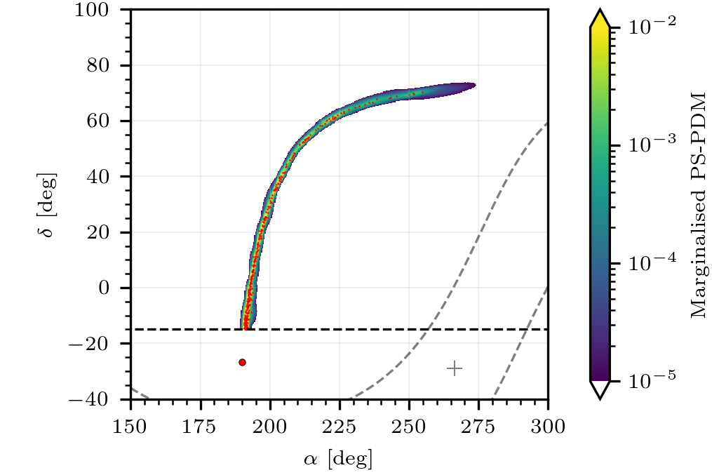
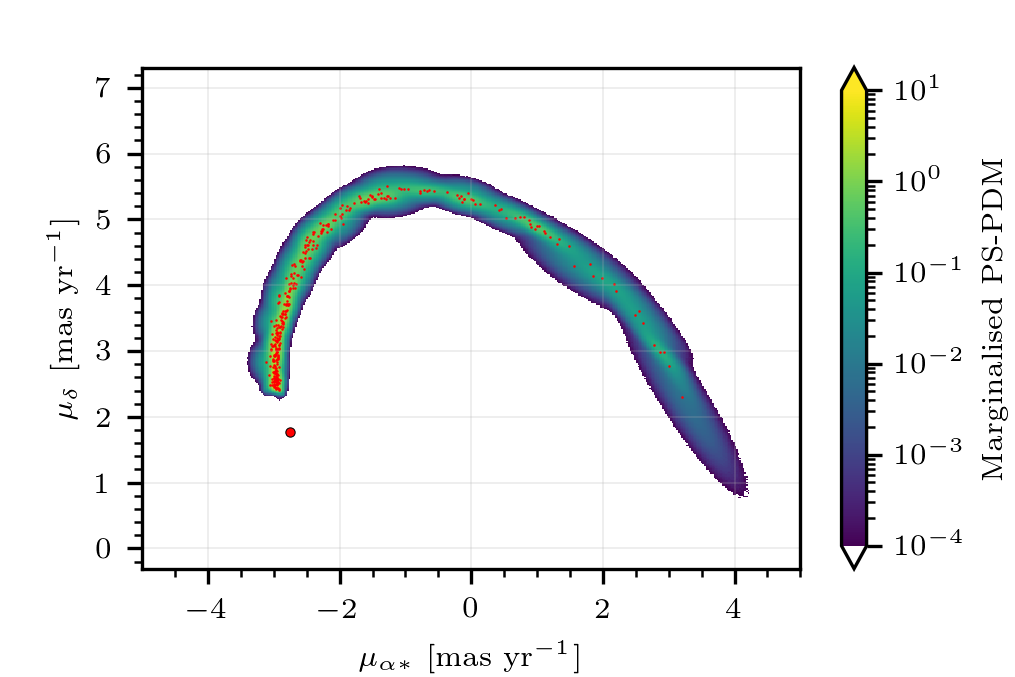
Figure 11: Marginalised phase-space probability density model of the M68 stream (PS-PDM), computed for the best-fitting parameters of the model with all streams together. The small red dots mark the positions of the simulated stars used to compute the density model, and the large red dot marks the position of the cluster. Top panel: Sky coordinates space. The horizontal black dashed line marks the $\delta=-15$ deg limit used to define the density model. The grey dashed lines mark the Milky Way disc at $b=\pm 15$ deg and the grey cross marks the Galactic centre. Bottom panel: Proper motions space.

Next, we assume that the observed stars $d_{\rm str}$ follow a Gaussian distribution centred at the mean phase-space position of the star $w^{\nu}$, where the covariance matrix $\varSigma^{\nu\epsilon}$ is the value of the observational errors and their correlations. If the stars do not have radial velocity we take $v_{r}=0\pm 10^{3}$ ${\rm km\,s}^{-1}$. This is a value with an uncertainty much bigger than the expected distribution of radial velocities of the stellar stream. It is almost equivalent to use a uniform distribution for the missing radial velocity, but simplifies the definition of the likelihood function. For the $j$ observed star we have:

$$\begin{split}\sum_{n=1}^{N}\,\int_{-\infty}^{\infty}G\mbox{\footnotesize$\big{(}w^{\nu}|\eta_{n}^{\nu},\varXi_{n}^{\nu\epsilon}\big{)}$}\,G\mbox{\footnotesize$\big{(}w^{\nu}|\nu_{j}^{\nu},\varSigma_{j}^{\nu\epsilon}\big{)}$}\mathop{}\!\mathrm{d}^{6}w=\\ =\sum_{n=1}^{N}G\mbox{\footnotesize$\big{(}\eta^{\nu}_{n}|\nu_{j}^{\nu},\varXi_{n}^{\nu\epsilon}+\varSigma_{j}^{\nu\epsilon}\big{)}$}~{}.\end{split}$$ (21)

If $J$ is the total number of observed stars in the stream, we get the following likelihood function:

$$\mathcal{L}_{\rm str}\mbox{\footnotesize$(d_{\rm str}|\theta)$}=\prod_{j=1}^{J}\sum_{n=1}^{N}G\mbox{\footnotesize$\big{(}\eta^{\nu}_{n}|\nu_{j}^{\nu},\varXi_{n}^{\nu\epsilon}+\varSigma_{j}^{\nu\epsilon}\big{)}$}~{}.$$ (22)

Appendix D Stream coordinates

To minimise the time required to evaluate the likelihood function, we apply a method to obtain an approximate distribution of stream stars from a pre-calculated simulation.

To carry out this simulation, we choose the mean position of the globular cluster and a fiducial potential of the Galaxy. We take the orbit of a globular cluster in Galactocentric Cartesian coordinates $x^{i}_{\rm o}$, where $i=(x,y,z)$, during $T$ Myr backwards and forwards from the present position of the cluster. We also take the current position of a simulated stream stars $x^{i}_{e}$. For each star $e$, we compute the closest point of the orbit to the star using an Euclidean distance. This point is expressed in function of the parameter $t$:

$$\hat{t}_{e}\equiv\operatorname*{argmin}_{t\in[-T,T]}\;\!\!\!\mbox{\footnotesize$\big{(}d_{e}\mbox{\footnotesize$(t)$}\big{)}$}~{},\qquad\,d^{\>\!2}_{e}\mbox{\footnotesize$(t)$}=\sum_{i=1}^{3}(x^{i}_{\rm o}\mbox{\footnotesize$(t)$}-x_{e}^{i})^{2}~{}.$$ (23)

Defining $v\equiv v^{i}_{\rm o}\mbox{\footnotesize$(\hat{t}_{e})$}$ as the velocity of the cluster and

$$a\equiv\dfrac{\mathop{}\!\mathrm{d}}{\mathop{}\!\mathrm{d}t}\dfrac{v}{|v|}~{},$$ (24)

and assuming $|v|>0$, $|a|>0$, and $|v\times a|>0$ for any $t$, we define the corresponding Frenet-Serret trihedron at the point $x^{i}_{\rm o}\mbox{\footnotesize$(\hat{t}_{e})$}$ as:

$$e_{1}=\frac{v}{|v|}~{},\qquad e_{2}=\frac{a}{|a|}~{},\qquad e_{3}=\frac{e_{1}\times e_{2}}{|e_{1}\times e_{2}|}~{}.$$ (25)

We store the parameter $\hat{t}_{e}$ and the position and velocity of the stream star expressed in the coordinate system defined by the vector basis $(e_{1},e_{2},e_{3})$.

When we evaluate the likelihood function for different values of the free parameters, we compute a new orbit of the cluster $\bar{x}_{\rm o}^{i}$. We assume that the stored values are independent of the orbit for small variations with respect to $x^{i}_{\rm o}$. Then, for each star $e$, we compute the Frenet-Serret trihedron corresponding to the position $\bar{x}_{\rm o}^{i}\mbox{\footnotesize$(\hat{t}_{e})$}$, and we locate the star at the stored values in the reference frame defined by the new trihedron $(\bar{e}_{1},\bar{e}_{2},\bar{e}_{3})$. Finally, we put back the stars on the Galactocentric Cartesian coordinate system to get an approximation of the stellar stream for the new values of the free parameters.

This method is based on the assumption that the internal structure of the stream and the offset between the stream and the cluster orbit does not change for small variations of the Galactic potential. We note that in action-angle coordinates, the misalignment angle between the stream and the cluster orbit is constant along the stream in the angle space (Eyre & Binney, 2011). For a small variation of the potential, for example a variation $\Delta q^{\rm h}_{\rho}\mathrel{\mathchoice{\raise 0.0pt\hbox{\scalebox{0.8}{\raise 0.0pt\hbox{$\displaystyle\sim$}}}}{\raise 0.0pt\hbox{\scalebox{0.8}{\raise 0.0pt\hbox{$\textstyle\sim$}}}}{\raise 0.0pt\hbox{\scalebox{0.8}{\raise 0.0pt\hbox{$\scriptstyle\sim$}}}}{\raise 0.0pt\hbox{\scalebox{0.8}{\raise 0.0pt\hbox{$\scriptscriptstyle\sim$}}}}}15$ per cent, we expect variations of the cluster radial action of $\Delta J_{R}\mathrel{\mathchoice{\raise 0.0pt\hbox{\scalebox{0.8}{\raise 0.0pt\hbox{$\displaystyle\sim$}}}}{\raise 0.0pt\hbox{\scalebox{0.8}{\raise 0.0pt\hbox{$\textstyle\sim$}}}}{\raise 0.0pt\hbox{\scalebox{0.8}{\raise 0.0pt\hbox{$\scriptstyle\sim$}}}}{\raise 0.0pt\hbox{\scalebox{0.8}{\raise 0.0pt\hbox{$\scriptscriptstyle\sim$}}}}}20$ per cent and of the vertical action $\Delta J_{z}\mathrel{\mathchoice{\raise 0.0pt\hbox{\scalebox{0.8}{\raise 0.0pt\hbox{$\displaystyle\sim$}}}}{\raise 0.0pt\hbox{\scalebox{0.8}{\raise 0.0pt\hbox{$\textstyle\sim$}}}}{\raise 0.0pt\hbox{\scalebox{0.8}{\raise 0.0pt\hbox{$\scriptstyle\sim$}}}}{\raise 0.0pt\hbox{\scalebox{0.8}{\raise 0.0pt\hbox{$\scriptscriptstyle\sim$}}}}}10$ per cent. Such variations of the actions will result in a negligible change in the misalignment angle, as well as in the length and width of the stream. This is exemplified by a numerical calculation for a realistic model of the Milky Way (McMillan, 2011) and a GD-1-like orbit in Figure 2 of Sanders & Binney (2013). When the stream is mapped to real space from the action-angle space, the constant misalignment angle translates into a constant offset between the stream and the cluster orbit.

Appendix E Halo flattening

In Table 5, we show the median with the $1\sigma$ levels and the mean with the standard deviation of the marginalised posterior probability density function of the axis ratio $q_{\rho}^{\rm h}$. We also include the best-fitting parameters of a log-Normal probability density function defined as:

$$\operatorname{logN}\!\mbox{\footnotesize$(x|\mu,\tau,\epsilon)$}\equiv\frac{1}{\sqrt{2\pi}(x-\mu)\tau}\exp\!\left[\frac{-\log\!\left(\frac{x-\mu}{\epsilon}\right)^{2}}{2\tau^{2}}\right]\,\,.$$ (26)

Table 5: Median with $1\sigma$ levels, mean and stardard deviation, and best-fitting parameters of a log-Normal distribution of the marginalised posterior probability density function of the flattening parameter $q_{\rho}^{\rm h}$.

	Median${}^{+\sigma}_{-\sigma}$	${\rm Mean}\,\,\,\,\,s$	$\hskip 18.99995pt\mu\hskip 18.50008pt\tau\hskip 20.00003pt\epsilon$
NGC 3201	$2.06_{-0.86}^{+1.01}$	$2.13\,\,\,\,0.88$	$-2.79\,\,\,\,0.18\,\,\,\,4.84$
M68	$1.14_{-0.14}^{+0.21}$	$1.17\,\,\,\,0.18$	+0$0.60\,\,\,\,0.31\,\,\,\,0.54$
Palomar 5	$1.01_{-0.09}^{+0.09}$	$1.01\,\,\,\,0.09$	$-8.18\,\,\,\,0.01\,\,\,\,9.19$
All	$1.06_{-0.05}^{+0.06}$	$1.07\,\,\,\,0.07$	+0$0.66\,\,\,\,0.16\,\,\,\,0.40$

Appendix F Numerical results

Table 6 lists the median and $1\sigma$ levels of the marginalised free parameters and derived properties of the Galaxy potential model. They are computed for each stream separately and for all streams together. Asymmetric errors are given when the difference between the upper and lower uncertainty is larger than 20 per cent.

Table 6: Gaussian priors, median and $1\sigma$ levels of the marginalised free parameters of our models. We include the value of the constraints described in Section 2 and 3, and several derived properties of the Milky Way model.

Parameter		Gaussian Prior	NGC 3201	M68	Palomar 5	All
$R_{\scalebox{0.7}{$\odot$}}$	(kpc)	$8.178\pm 0.026$	$8.17\pm 0.02$	$8.17\pm 0.03$	$8.14\pm 0.03$	$8.15_{-0.03}^{+0.02}$
$U_{\scalebox{0.7}{$\odot$}}$	(km s-1)	$11.1\pm 1.25$	$9.61\pm 1.01$	$9.89\pm 0.97$	$12.47\pm 1.27$	$10.58_{-0.42}^{+0.89}$
$V_{\scalebox{0.7}{$\odot$}}$	(km s-1)	$12.24\pm 2.05$	$14.58\pm 1.43$	$15.24\pm 1.56$	$13.39\pm 1.57$	$13.64_{-1.2}^{+1.84}$
$W_{\scalebox{0.7}{$\odot$}}$	(km s-1)	$7.25\pm 0.62$	$7.61\pm 0.56$	$7.45\pm 0.59$	$7.22\pm 0.64$	$7.33\pm 0.51$
$\rho_{0}^{\rm b}$	($10^{10}\,$M${}_{\scalebox{0.7}{$\odot$}}$ kpc-3)		$9.80\pm 1.02$	$9.62\pm 1.03$	$9.97_{-1.08}^{+0.78}$	$9.84_{-0.95}^{+0.69}$
$\varSigma_{\rm n}$	($10^{9}\,$M${}_{\scalebox{0.7}{$\odot$}}$ kpc-2)		$0.92\pm 0.22$	$1.19\pm 0.13$	$0.9_{-0.15}^{+0.21}$	$1.25_{-0.2}^{+0.14}$
$h_{\rm n}$	(kpc)	$2.6\pm 0.5$	$3.01_{-0.23}^{+0.29}$	$2.88_{-0.14}^{+0.21}$	$2.99\pm 0.25$	$2.78_{-0.1}^{+0.18}$
$z_{\rm n}$	(kpc)	$0.3\pm 0.05$	$0.31\pm 0.05$	$0.30\pm 0.05$	$0.31\pm 0.05$	$0.31_{-0.03}^{+0.04}$
$\varSigma_{\rm k}$	($10^{8}\,$M${}_{\scalebox{0.7}{$\odot$}}$ kpc-2)		$4.17_{-1.66}^{+2.66}$	$4.75\pm 2.06$	$4.25_{-1.7}^{+2.39}$	$3.77_{-1.37}^{+2.44}$
$h_{\rm k}$	(kpc)	$2.0\pm 0.2$	$1.97\pm 0.19$	$1.98\pm 0.18$	$1.93\pm 0.18$	$2.06_{-0.21}^{+0.14}$
$z_{\rm k}$	(kpc)	$0.9\pm 0.18$	$0.93\pm 0.16$	$0.90\pm 0.18$	$0.91\pm 0.17$	$0.79_{-0.12}^{+0.25}$
$\rho_{0}^{\rm h}$	($10^{7}\,$M${}_{\scalebox{0.7}{$\odot$}}$ kpc-3)		$1.92_{-1.6}^{+2.85}$	$2.94_{-1.44}^{+2.22}$	$2.0_{-1.5}^{+2.88}$	$1.84_{-0.62}^{+1.05}$
$\alpha$			$0.68\pm 0.64$	$-0.23\pm 0.39$	$0.73\pm 0.45$	$0.06\pm 0.22$
$a_{1}$	(kpc)		$12.58_{-6.13}^{+20.06}$	$18.63_{-5.41}^{+10.08}$	$11.22_{-5.1}^{+17.14}$	$17.36_{-2.74}^{+9.77}$
$\beta$			$3.19_{-0.61}^{+1.19}$	$3.73_{-0.56}^{+0.83}$	$2.77_{-0.33}^{+0.93}$	$3.29_{-0.28}^{+0.66}$
$q_{\rho}^{\rm h}$			$2.06\pm 0.93$	$1.14_{-0.14}^{+0.21}$	$1.01\pm 0.09$	$1.06\pm 0.06$
$r_{\rm h}^{{\scaleto{\rm NGC3201}{3.5pt}}}$	(kpc)	$4.9\pm 0.11$	$4.82\pm 0.02$			$4.83\pm 0.02$
$v_{r}^{{\scaleto{\rm NGC3201}{3.5pt}}}$	(km s-1)	$494.34\pm 0.14$	$494.32\pm 0.14$			$494.31\pm 0.13$
$\mu_{\delta}^{{\scaleto{\rm NGC3201}{3.5pt}}}$	(mas yr-1)	$-1.991\pm 0.044$	$-1.962\pm 0.023$			$-1.931_{-0.019}^{+0.03}$
$\mu_{\alpha*}^{{\scaleto{\rm NGC3201}{3.5pt}}}$	(mas yr-1)	$8.324\pm 0.044$	$8.309\pm 0.042$			$8.293\pm 0.056$
$r_{\rm h}^{{\scaleto{\rm M68}{3.5pt}}}$	(kpc)	$10.3\pm 0.52$		$10.01_{-0.11}^{+0.08}$		$10.03\pm 0.06$
$v_{r}^{{\scaleto{\rm M68}{3.5pt}}}$	(km s-1)	$-92.99\pm 0.22$		$-92.95\pm 0.22$		$-92.9_{-0.29}^{+0.2}$
$\mu_{\delta}^{{\scaleto{\rm M68}{3.5pt}}}$	(mas yr-1)	$1.762\pm 0.053$		$1.766\pm 0.027$		$1.782\pm 0.027$
$\mu_{\alpha*}^{{\scaleto{\rm M68}{3.5pt}}}$	(mas yr-1)	$-2.752\pm 0.054$		$-2.750\pm 0.028$		$-2.744_{-0.026}^{+0.02}$
$r_{\rm h}^{{\scaleto{\rm Palomar\,5}{3.5pt}}}$	(kpc)	$20.6\pm 0.2$			$21.19\pm 0.15$	$21.20\pm 0.15$
$v_{r}^{{\scaleto{\rm Palomar\,5}{3.5pt}}}$	(km s-1)	$-58.6\pm 0.21$			$-58.44\pm 0.20$	$-58.5_{-0.12}^{+0.17}$
$\mu_{\delta}^{{\scaleto{\rm Palomar\,5}{3.5pt}}}$	(mas yr-1)	$-2.646\pm 0.064$			$-2.546\pm 0.016$	$-2.544_{-0.018}^{+0.013}$
$\mu_{\alpha*}^{{\scaleto{\rm Palomar\,5}{3.5pt}}}$	(mas yr-1)	$-2.736\pm 0.064$			$-2.533\pm 0.017$	$-2.513_{-0.02}^{+0.015}$

Table 6: - continued

Parameter		Gaussian Prior	NGC 3201	M68	Palomar 5	All
$f_{\varSigma}$		$0.12\pm 0.04$	$0.11\pm 0.03$	$0.11\pm 0.04$	$0.11\pm 0.03$	$0.11\pm 0.03$
$K_{z}$	($2\pi G$ M${}_{\scalebox{0.7}{$\odot$}}$ pc-2)	$74\pm 6$	$77.58\pm 4.73$	$88.49\pm 4.31$	$80.37\pm 5.47$	$86.81_{-3.84}^{+2.93}$
	(km2 pc-1 s-2)	$2\pm 0.16$	$2.10\pm 0.13$	$2.39\pm 0.12$	$2.17\pm 0.15$	$2.33\pm 0.09$
$\mu_{l}$	(mas yr-1)	$-6.379\pm 0.026$	$-6.37\pm 0.02$	$-6.35\pm 0.02$	$-6.33\pm 0.02$	$-6.32\pm 0.02$
$\Theta_{0}$	(km s-1)		$232.39\pm 1.38$	$230.70\pm 1.44$	$230.79\pm 1.48$	$230.67\pm 1.55$
$\Theta_{0}+V_{\scalebox{0.7}{$\odot$}}$	(km s-1)		$246.95\pm 1.14$	$245.92\pm 1.14$	$244.15\pm 1.12$	$244.38\pm 0.91$
$V_{\rm c}\,\scalebox{0.8}{(R\,=\,5.27\,{\rm kpc})}$	(km s-1)	$226.83\pm 7.07$	$230.74\pm 2.8$	$230.11\pm 2.92$	$229.49\pm 2.58$	$231.1_{-3.51}^{+2.32}$
$V_{\rm c}\,\scalebox{0.8}{(R\,=\,10.26\,{\rm kpc})}$	(km s-1)	$225.68\pm 6.78$	$227.82\pm 1.28$	$225.38\pm 1.25$	$226.18\pm 1.28$	$224.85_{-1.32}^{+0.98}$
$V_{\rm c}\,\scalebox{0.8}{(R\,=\,15.22\,{\rm kpc})}$	(km s-1)	$217.07\pm 6.58$	$214.55\pm 1.4$	$212.71\pm 1.35$	$213.33\pm 1.32$	$211.43_{-1.28}^{+1.64}$
$V_{\rm c}\,\scalebox{0.8}{(R\,=\,20.27\,{\rm kpc})}$	(km s-1)	$199.84\pm 6.71$	$204.72\pm 1.92$	$205.66\pm 1.95$	$204.02\pm 1.96$	$204.88\pm 2.2$
$V_{\rm c}\,\scalebox{0.8}{(R\,=\,24.82\,{\rm kpc})}$	(km s-1)	$198.42\pm 8.67$	$198.76\pm 2.94$	$202.52\pm 2.84$	$198.54\pm 2.94$	$202.2_{-3.3}^{+2.45}$
$M_{\rm b}$	($10^{9}\,$M${}_{\scalebox{0.7}{$\odot$}}$)	$8.9\pm 0.89$	$8.84\pm 0.92$	$8.68\pm 0.93$	$9.0_{-0.97}^{+0.71}$	$8.87_{-0.86}^{+0.62}$
$M_{\rm d}^{\rm n}$	($10^{10}\,$M${}_{\scalebox{0.7}{$\odot$}}$)		$5.26\pm 0.60$	$6.22\pm 0.40$	$5.13\pm 0.56$	$6.07\pm 0.39$
$M_{\rm d}^{\rm k}$	($10^{10}\,$M${}_{\scalebox{0.7}{$\odot$}}$)		$1.02\pm 0.36$	$1.16\pm 0.39$	$1.00\pm 0.36$	$1.01_{-0.29}^{+0.4}$
$M_{{\rm bar}}$	($10^{10}\,$M${}_{\scalebox{0.7}{$\odot$}}$)		$7.22\pm 0.70$	$8.30\pm 0.49$	$7.04\pm 0.66$	$8.01\pm 0.38$
$M^{\rm h}_{200}$	($10^{12}\,$M${}_{\scalebox{0.7}{$\odot$}}$)		$0.95\pm 0.23$	$0.94\pm 0.22$	$0.94\pm 0.24$	$1.08\pm 0.22$
$M_{200}$	($10^{12}\,$M${}_{\scalebox{0.7}{$\odot$}}$)		$1.03\pm 0.23$	$1.03\pm 0.23$	$1.02\pm 0.25$	$1.18\pm 0.23$
$\rho_{\rm h}\mbox{\footnotesize$(R_{\scalebox{0.7}{$\odot$}})$}$	($10^{6}\,$M${}_{\scalebox{0.7}{$\odot$}}$ kpc-3)		$5.2_{-0.77}^{+1.87}$	$5.66\pm 0.84$	$7.43\pm 0.86$	$5.95\pm 0.60$
	(GeV cm-3)		$0.2_{-0.03}^{+0.07}$	$0.21\pm 0.03$	$0.28\pm 0.03$	$0.23\pm 0.02$
$r_{200}$	(kpc)		$200.56\pm 16.38$	$199.89_{-19.16}^{+13.52}$	$199.85\pm 17.33$	$209.6_{-16.71}^{+12.79}$
$c_{200}$			$13.48_{-3.06}^{+4.82}$	$8.24\pm 0.58$	$10.43_{-1.92}^{+2.95}$	$7.86_{-0.44}^{+0.57}$

References

- Astropy Collaboration et al. (2022) Astropy Collaboration et al., 2022, ApJ, 935, 167
- Bailin et al. (2005) Bailin J., et al., 2005, ApJ, 627, L17
- Baumgardt & Vasiliev (2021) Baumgardt H., Vasiliev E., 2021, MNRAS, 505, 5957
- Baumgardt et al. (2019) Baumgardt H., Hilker M., Sollima A., Bellini A., 2019, MNRAS, 482, 5138
- Belokurov et al. (2006) Belokurov V., Evans N. W., Irwin M. J., Hewett P. C., Wilkinson M. I., 2006, ApJ, 637, L29
- Belokurov et al. (2014) Belokurov V., et al., 2014, MNRAS, 437, 116
- Bienaymé et al. (2014) Bienaymé O., et al., 2014, A&A, 571, A92
- Binney & Tremaine (2008) Binney J., Tremaine S., 2008, Galactic Dynamics: Second Edition. Princeton University Press
- Bissantz & Gerhard (2002) Bissantz N., Gerhard O., 2002, MNRAS, 330, 591
- Bland-Hawthorn & Gerhard (2016) Bland-Hawthorn J., Gerhard O., 2016, ARA&A, 54, 529
- Bonaca et al. (2014) Bonaca A., Geha M., Küpper A. H. W., Diemand J., Johnston K. V., Hogg D. W., 2014, ApJ, 795, 94
- Bonaca et al. (2020) Bonaca A., et al., 2020, ApJ, 889, 70
- Bovy (2014) Bovy J., 2014, ApJ, 795, 95
- Bovy & Rix (2013) Bovy J., Rix H.-W., 2013, ApJ, 779, 115
- Bovy et al. (2015) Bovy J., Bird J. C., García Pérez A. E., Majewski S. R., Nidever D. L., Zasowski G., 2015, ApJ, 800, 83
- Bovy et al. (2016) Bovy J., Bahmanyar A., Fritz T. K., Kallivayalil N., 2016, ApJ, 833, 31
- Bowden et al. (2015) Bowden A., Belokurov V., Evans N. W., 2015, MNRAS, 449, 1391
- Bowden et al. (2016) Bowden A., Evans N. W., Williams A. A., 2016, MNRAS, 460, 329
- Bryan et al. (2013) Bryan S. E., Kay S. T., Duffy A. R., Schaye J., Dalla Vecchia C., Booth C. M., 2013, MNRAS, 429, 3316
- Butsky et al. (2016) Butsky I., et al., 2016, MNRAS, 462, 663
- Callingham et al. (2019) Callingham T. M., et al., 2019, MNRAS, 484, 5453
- Carlberg et al. (2012) Carlberg R. G., Grillmair C. J., Hetherington N., 2012, ApJ, 760, 75
- Cautun et al. (2020) Cautun M., et al., 2020, MNRAS, 494, 4291
- Chua et al. (2019) Chua K. T. E., Pillepich A., Vogelsberger M., Hernquist L., 2019, MNRAS, 484, 476
- Clarke et al. (2019) Clarke J. P., Wegg C., Gerhard O., Smith L. C., Lucas P. W., Wylie S. M., 2019, MNRAS, 489, 3519
- Dai et al. (2018) Dai B., Robertson B. E., Madau P., 2018, ApJ, 858, 73
- De Martino et al. (2020) De Martino I., Broadhurst T., Henry Tye S. H., Chiueh T., Schive H.-Y., 2020, Physics of the Dark Universe, 28, 100503
- DeBuhr et al. (2012) DeBuhr J., Ma C.-P., White S. D. M., 2012, MNRAS, 426, 983
- Debattista et al. (2013) Debattista V. P., Roškar R., Valluri M., Quinn T., Moore B., Wadsley J., 2013, MNRAS, 434, 2971
- Deg & Widrow (2013) Deg N., Widrow L., 2013, MNRAS, 428, 912
- Eilers et al. (2019) Eilers A.-C., Hogg D. W., Rix H.-W., Ness M. K., 2019, ApJ, 871, 120
- Erkal & Belokurov (2020) Erkal D., Belokurov V. A., 2020, MNRAS, 495, 2554
- Erkal et al. (2019) Erkal D., et al., 2019, MNRAS, 487, 2685
- Eyre & Binney (2011) Eyre A., Binney J., 2011, MNRAS, 413, 1852
- Fardal et al. (2015) Fardal M. A., Huang S., Weinberg M. D., 2015, MNRAS, 452, 301
- Fardal et al. (2019) Fardal M. A., van der Marel R. P., Law D. R., Sohn S. T., Sesar B., Hernitschek N., Rix H.-W., 2019, MNRAS, 483, 4724
- Fellhauer et al. (2006) Fellhauer M., et al., 2006, ApJ, 651, 167
- Gaia Collaboration et al. (2016) Gaia Collaboration et al., 2016, A&A, 595, A1
- Gaia Collaboration et al. (2018) Gaia Collaboration et al., 2018, A&A, 616, A1
- Gardner et al. (2020) Gardner S., Hinkel A., Yanny B., 2020, ApJ, 890, 110
- Gravity Collaboration et al. (2019) Gravity Collaboration et al., 2019, A&A, 625, L10
- Grillmair (2019) Grillmair C. J., 2019, ApJ, 884, 174
- Grillmair & Carlin (2016) Grillmair C. J., Carlin J. L., 2016, in Newberg H. J., Carlin J. L., eds, Astrophysics and Space Science Library Vol. 420, Tidal Streams in the Local Group and Beyond. p. 87 (arXiv:1603.08936), doi:10.1007/978-3-319-19336-6_4
- Grillmair & Johnson (2006) Grillmair C. J., Johnson R., 2006, ApJ, 639, L17
- Harris (1996) Harris W. E., 1996, AJ, 112, 1487
- Harris (2010) Harris W. E., 2010, arXiv e-prints, p. arXiv:1012.3224
- Harris et al. (2020) Harris C. R., et al., 2020, Nature, 585, 357
- Hattori & Valluri (2020) Hattori K., Valluri M., 2020, in Valluri M., Sellwood J. A., eds, Vol. 353, Galactic Dynamics in the Era of Large Surveys. pp 96–100 (arXiv:1909.03321), doi:10.1017/S1743921319008718
- Hattori et al. (2021) Hattori K., Valluri M., Vasiliev E., 2021, MNRAS, 508, 5468
- Hawkins et al. (2023) Hawkins K., et al., 2023, ApJ, 948, 123
- Helmi (2004) Helmi A., 2004, ApJ, 610, L97
- Holmberg & Flynn (2004) Holmberg J., Flynn C., 2004, MNRAS, 352, 440
- Huang et al. (2016) Huang Y., et al., 2016, MNRAS, 463, 2623
- Hunter (2007) Hunter J. D., 2007, Computing in Science & Engineering, 9, 90
- Ibata et al. (2001) Ibata R., Lewis G. F., Irwin M., Totten E., Quinn T., 2001, ApJ, 551, 294
- Ibata et al. (2013) Ibata R., Lewis G. F., Martin N. F., Bellazzini M., Correnti M., 2013, ApJ, 765, L15
- Ibata et al. (2016) Ibata R. A., Lewis G. F., Martin N. F., 2016, ApJ, 819, 1
- Ibata et al. (2017) Ibata R. A., Lewis G. F., Thomas G., Martin N. F., Chapman S., 2017, ApJ, 842, 120
- Ibata et al. (2018) Ibata R. A., Malhan K., Martin N. F., Starkenburg E., 2018, ApJ, 865, 85
- Ibata et al. (2019a) Ibata R. A., Bellazzini M., Malhan K., Martin N., Bianchini P., 2019a, Nature Astronomy, 3, 667
- Ibata et al. (2019b) Ibata R. A., Malhan K., Martin N. F., 2019b, ApJ, 872, 152
- Jensen et al. (2021) Jensen J., et al., 2021, MNRAS, 507, 1923
- Johansson et al. (2017) Johansson F., et al., 2017, Mpmath: A Python Library For Arbitrary-Precision Floating-Point Arithmetic, Zenodo, doi:10.5281/zenodo.1476881
- Johnston et al. (2005) Johnston K. V., Law D. R., Majewski S. R., 2005, ApJ, 619, 800
- Jurić et al. (2008) Jurić M., et al., 2008, ApJ, 673, 864
- Just & Jahreiß (2010) Just A., Jahreiß H., 2010, MNRAS, 402, 461
- Kafle et al. (2012) Kafle P. R., Sharma S., Lewis G. F., Bland -Hawthorn J., 2012, ApJ, 761, 98
- Koposov et al. (2010) Koposov S. E., Rix H.-W., Hogg D. W., 2010, ApJ, 712, 260
- Kuijken & Gilmore (1991) Kuijken K., Gilmore G., 1991, ApJ, 367, L9
- Küpper et al. (2008) Küpper A. H. W., MacLeod A., Heggie D. C., 2008, MNRAS, 387, 1248
- Küpper et al. (2012) Küpper A. H. W., Lane R. R., Heggie D. C., 2012, MNRAS, 420, 2700
- Küpper et al. (2015) Küpper A. H. W., Balbinot E., Bonaca A., Johnston K. V., Hogg D. W., Kroupa P., Santiago B. X., 2015, ApJ, 803, 80
- Kuzma et al. (2015) Kuzma P. B., Da Costa G. S., Keller S. C., Maunder E., 2015, MNRAS, 446, 3297
- Lane et al. (2010) Lane R. R., et al., 2010, MNRAS, 406, 2732
- Law & Majewski (2010) Law D. R., Majewski S. R., 2010, ApJ, 714, 229
- Law et al. (2009) Law D. R., Majewski S. R., Johnston K. V., 2009, ApJ, 703, L67
- Li et al. (2020) Li P., Lelli F., McGaugh S., Schombert J., 2020, ApJS, 247, 31
- Loebman et al. (2012) Loebman S. R., Ivezić Ž., Quinn T. R., Governato F., Brooks A. M., Christensen C. R., Jurić M., 2012, ApJ, 758, L23
- Loebman et al. (2014) Loebman S. R., et al., 2014, ApJ, 794, 151
- López-Corredoira (2014) López-Corredoira M., 2014, A&A, 563, A128
- Luna et al. (2006) Luna A., Bronfman L., Carrasco L., May J., 2006, ApJ, 641, 938
- Luri et al. (2014) Luri X., et al., 2014, A&A, 566, A119
- MacKay (2003) MacKay D. J. C., 2003, Information Theory, Inference, and Learning Algorithms. Copyright Cambridge University Press
- Malhan & Ibata (2019) Malhan K., Ibata R. A., 2019, MNRAS, 486, 2995
- Malhan et al. (2018) Malhan K., Ibata R. A., Martin N. F., 2018, MNRAS, 481, 3442
- Malhan et al. (2019) Malhan K., Ibata R. A., Carlberg R. G., Valluri M., Freese K., 2019, ApJ, 881, 106
- Mateu (2023) Mateu C., 2023, MNRAS, 520, 5225
- McClure-Griffiths & Dickey (2007) McClure-Griffiths N. M., Dickey J. M., 2007, ApJ, 671, 427
- McClure-Griffiths & Dickey (2016) McClure-Griffiths N. M., Dickey J. M., 2016, ApJ, 831, 124
- McMillan (2011) McMillan P. J., 2011, MNRAS, 414, 2446
- McMillan (2017) McMillan P. J., 2017, MNRAS, 465, 76
- Mróz et al. (2019) Mróz P., et al., 2019, ApJ, 870, L10
- Navarro et al. (1996) Navarro J. F., Frenk C. S., White S. D. M., 1996, ApJ, 462, 563
- Nitschai et al. (2020) Nitschai M. S., Cappellari M., Neumayer N., 2020, MNRAS, 494, 6001
- Odenkirchen et al. (2001) Odenkirchen M., et al., 2001, ApJ, 548, L165
- Palau & Miralda-Escudé (2019) Palau C. G., Miralda-Escudé J., 2019, MNRAS, 488, 1535
- Palau & Miralda-Escudé (2021) Palau C. G., Miralda-Escudé J., 2021, MNRAS, 504, 2727
- Patel et al. (2020) Patel E., et al., 2020, ApJ, 893, 121
- Pearson et al. (2015) Pearson S., Küpper A. H. W., Johnston K. V., Price-Whelan A. M., 2015, ApJ, 799, 28
- Piatti & Carballo-Bello (2020) Piatti A. E., Carballo-Bello J. A., 2020, A&A, 637, L2
- Portail et al. (2015) Portail M., Wegg C., Gerhard O., Martinez-Valpuesta I., 2015, MNRAS, 448, 713
- Prada et al. (2019) Prada J., Forero-Romero J. E., Grand R. J. J., Pakmor R., Springel V., 2019, MNRAS, 490, 4877
- Price-Whelan et al. (2014) Price-Whelan A. M., Hogg D. W., Johnston K. V., Hendel D., 2014, ApJ, 794, 4
- Price-Whelan et al. (2019) Price-Whelan A. M., Mateu C., Iorio G., Pearson S., Bonaca A., Belokurov V., 2019, AJ, 158, 223
- Reid & Brunthaler (2004) Reid M. J., Brunthaler A., 2004, ApJ, 616, 872
- Reid et al. (2019) Reid M. J., et al., 2019, ApJ, 885, 131
- Salucci (2019) Salucci P., 2019, A&ARv, 27, 2
- Sanders & Binney (2013) Sanders J. L., Binney J., 2013, MNRAS, 433, 1813
- Schönrich et al. (2010) Schönrich R., Binney J., Dehnen W., 2010, MNRAS, 403, 1829
- Shao et al. (2016) Shao S., Cautun M., Frenk C. S., Gao L., Crain R. A., Schaller M., Schaye J., Theuns T., 2016, MNRAS, 460, 3772
- Shipp et al. (2018) Shipp N., et al., 2018, ApJ, 862, 114
- Shipp et al. (2020) Shipp N., Price-Whelan A. M., Tavangar K., Mateu C., Drlica-Wagner A., 2020, AJ, 160, 244
- Shipp et al. (2021) Shipp N., et al., 2021, ApJ, 923, 149
- Sollima & Baumgardt (2017) Sollima A., Baumgardt H., 2017, MNRAS, 471, 3668
- Starkman et al. (2020) Starkman N., Bovy J., Webb J. J., 2020, MNRAS, 493, 4978
- Tomassetti et al. (2016) Tomassetti M., et al., 2016, MNRAS, 458, 4477
- Varghese et al. (2011) Varghese A., Ibata R., Lewis G. F., 2011, MNRAS, 417, 198
- Vasiliev (2019a) Vasiliev E., 2019a, MNRAS, 482, 1525
- Vasiliev (2019b) Vasiliev E., 2019b, MNRAS, 484, 2832
- Vasiliev et al. (2021) Vasiliev E., Belokurov V., Erkal D., 2021, MNRAS, 501, 2279
- Velliscig et al. (2015) Velliscig M., et al., 2015, MNRAS, 453, 721
- Virtanen et al. (2020) Virtanen P., et al., 2020, Nature Methods, 17, 261
- Vogelsberger et al. (2020) Vogelsberger M., Marinacci F., Torrey P., Puchwein E., 2020, Nature Reviews Physics, 2, 42
- Wang et al. (2020) Wang W., Han J., Cautun M., Li Z., Ishigaki M. N., 2020, Science China Physics, Mechanics, and Astronomy, 63, 109801
- Wechsler & Tinker (2018) Wechsler R. H., Tinker J. L., 2018, ARA&A, 56, 435
- Wegg et al. (2015) Wegg C., Gerhard O., Portail M., 2015, MNRAS, 450, 4050
- Wegg et al. (2019) Wegg C., Gerhard O., Bieth M., 2019, MNRAS, 485, 3296
- Woudenberg et al. (2023) Woudenberg H. C., Koop O., Balbinot E., Helmi A., 2023, A&A, 669, A102
- Yang et al. (2022) Yang Y., Zhao J.-K., Ishigaki M. N., Zhou J.-Z., Yang C.-Q., Xue X.-X., Ye X.-H., Zhao G., 2022, MNRAS, 513, 853
- Zhang et al. (2013) Zhang L., Rix H.-W., van de Ven G., Bovy J., Liu C., Zhao G., 2013, ApJ, 772, 108
- de Boer et al. (2020) de Boer T. J. L., Erkal D., Gieles M., 2020, MNRAS, 494, 5315
- de Salas (2020) de Salas P. F., 2020, in Journal of Physics Conference Series. p. 012020 (arXiv:1910.14366), doi:10.1088/1742-6596/1468/1/012020