Primordial black holes generated by the non-minimal spectator field

Abstract

We improve and generalize the non-minimal curvaton model originally proposed in arXiv:2112.12680 to a model in which a spectator field non-minimally couples to an inflaton field and the power spectrum of the perturbation of spectator field at small scales is dramatically enhanced by the sharp feature in the form of non-minimal coupling. At or after the end of inflation, the perturbation of the spectator field is converted into curvature perturbation and leads to the formation of primordial black holes (PBHs). Furthermore, for example, we consider three phenomenological models for generating PBHs with mass function peaked at $\sim 10^{-12}M_{\odot}$ and representing all the cold dark matter in our Universe and find that the scalar induced gravitational waves generated by the curvature perturbation can be detected by the future space-borne gravitational-wave detectors such as Taiji, TianQin and LISA.

I Introduction

Primordial black holes (PBHs) formed from the collapse of large density perturbations in the very early universe Zel’dovich and Novikov (1967); Hawking (1971); Carr and Hawking (1974); Carr (1975) can contribute to the cold dark matter (CDM) and provide a possible explanation Bird et al. (2016); Sasaki et al. (2016); Clesse and García-Bellido (2017); Wang et al. (2018); Ali-Haïmoud et al. (2017); Chen and Huang (2018); Chen et al. (2019); Kavanagh et al. (2018); Raidal et al. (2019); Liu et al. (2019a); Chen and Huang (2020); Yuan et al. (2019a); Liu et al. (2019b); De Luca et al. (2021); Vattis et al. (2020); Wang and Zhao (2022); Chen et al. (2022) to the gravitational-wave (GW) events from the mergers of binary black holes detected by LIGO-Virgo collaboration Abbott et al. (2016, 2021).

Currently, various independent observations Carr et al. (2010); Graham et al. (2015); Niikura et al. (2019a); Tisserand et al. (2007); Niikura et al. (2019b); Wang et al. (2018); Chen and Huang (2020); Brandt (2016); Chen et al. (2020a); Montero-Camacho et al. (2019); Laha (2019); Dasgupta et al. (2020); Laha et al. (2020); Saha and Laha (2022); Ray et al. (2021) have placed upper limits at the percent level on the fraction of PBHs in CDM, leaving only two mass windows $\sim[10^{-16},10^{-14}]M_{\odot}$ and $\sim[10^{-13},10^{-12}]M_{\odot}$ where PBHs may still constitute all the CDM. See some recent reviews in Carr et al. (2020); Escrivà et al. (2022). In order to produce a sizable amount of PBHs to explain most of the CDM, the amplitude of the power spectrum $\mathcal{P}_{\zeta}$ of curvature perturbation should be significantly enhanced to $\mathcal{O}(10^{-2})$ on small scales from $\mathcal{O}(10^{-9})$ on the cosmic microwave background (CMB) scales Aghanim et al. (2020). Such an enhancement of the curvature power spectrum on small scales can be realized in many scenarios, including single-field inflation models Yokoyama (1998); Kinney (2005); Choudhury and Mazumdar (2014); Garcia-Bellido et al. (2016); Cheng et al. (2017); Garcia-Bellido and Ruiz Morales (2017); Cheng et al. (2018); Dalianis et al. (2019); Tada and Yokoyama (2019); Xu et al. (2020); Mishra and Sahni (2020); Bhaumik and Jain (2020); Liu et al. (2020); Atal et al. (2020); Fu et al. (2020); Vennin (2020); Ragavendra et al. (2020); Gao and Yang (2021); Cai et al. (2022); Karam et al. (2022); Di and Gong (2018); Cai et al. (2018); Chen et al. (2020b); Cai et al. (2019a, 2020); Cotner and Kusenko (2017a, b); Cotner et al. (2018, 2019); Escrivà and Subils (2022); Pi and Wang (2022); Garcia-Bellido and Ruiz Morales (2017); Germani and Prokopec (2017); Byrnes et al. (2019); Passaglia et al. (2019); Fu et al. (2019a, b); Liu et al. (2020); Fu et al. (2020); Inomata et al. (2022a); Tasinato (2021); Ragavendra et al. (2020); Cole et al. (2022); Karam et al. (2022); Fu and Wang (2022); Peng et al. (2021); Zhai et al. (2022); Kannike et al. (2017); Gao and Guo (2018); Cheong et al. (2021, 2020); Fu et al. (2019a); Dalianis et al. (2020); Fu et al. (2019b); Martin et al. (2020a, b); Lin et al. (2020); Yi et al. (2020); Gao et al. (2020); Gao (2021); Wu et al. (2021); Teimoori et al. (2021); Kawai and Kim (2021); Zhang (2022); Yi (2022); Gu et al. (2022); Cook (2022); Hidalgo et al. (2022); Animali and Vennin (2022); Fu and Wang (2022); Papanikolaou et al. (2022); Braglia et al. (2022); Kawaguchi and Tsujikawa (2022); Ashoorioon et al. (2021a); Fu and Chen (2022); Ahmed et al. (2022) and multi-field models Garcia-Bellido et al. (1996); Kawasaki et al. (1998); Yokoyama (1997); Frampton et al. (2010); Giovannini (2010); Clesse and García-Bellido (2015); Inomata et al. (2017a, 2018); Espinosa et al. (2018a); Kawasaki et al. (2020); Palma et al. (2020); Fumagalli et al. (2020); Braglia et al. (2020a); Anguelova (2021); Romano (2020); Gundhi and Steinwachs (2021); Gundhi et al. (2021); Cai et al. (2021); Ishikawa and Ketov (2022); Spanos and Stamou (2021); Hooshangi et al. (2022); Chen and Cai (2019); Fu and Chen (2022); Kohri et al. (2013); Kawasaki et al. (2013); Pi et al. (2018); Liu (2021); Pi and Sasaki (2021); Hooshangi et al. (2022); Kawai and Kim (2022); Ashoorioon et al. (2021b, 2022), etc. Usually the enhancement of the power spectrum of curvature perturbation at small scales may lead to a non-Gaussian distribution for the curvature perturbation. According to the explicit calculation of the one-loop correction to the power spectrum of curvature perturbation with local-type non-Guassianity, we conclude that the enhanced curvature perturbation for the formation of PBHs should be nearly Gaussian Meng et al. (2022); otherwise, the power spectrum will be dominated by the one-loop correction and then the perturbed description of curvature perturbation breaks down. Even though we only focus on the local-type non-Gaussianity, our conclusion is expected to be qualitatively reliable for the non-local-type non-Gaussianity as well. Along this line of thought, the single-field inflation models for the formation of PBHs might have been ruled out Kristiano and Yokoyama (2022a); Inomata et al. (2022b), or the scenario is not reliable at least. See more recent discussions in Riotto (2023); Choudhury et al. (2023).

Even though the minimally coupled multi-field inflation has been widely explored, the non-minimally coupled multi-field inflation is also attracted much attention in literature, e.g. Lalak et al. (2007); van de Bruck and Robinson (2014); Braglia et al. (2020b); Cai et al. (2021). Recently, a curvaton model with a sharp dip in the non-minimal coupling $f(\phi)$ is originally proposed in Pi and Sasaki (2021) where the perturbation of such a curvaton field is supposed to be enhanced by the inverse of $f(\phi)$ and peaked around the mode $k=k_{*}$ stretching outside the horizon at the dip. In this paper, we improve and generalize the non-minimal curvaton model to more general non-minimal spectator field model. The main differences of our model from Pi and Sasaki (2021) are:
1) Considering that the non-minimal coupling dramatically changes the perturbation equation of the spectator field, we numerically solve the perturbation equation and find that the shape, peak location and magnification of spectator field perturbation are quite different from those given in Pi and Sasaki (2021).
2) The perturbation of the non-minimal spectator field can be amplified by not only the sharp dip proposed in Pi and Sasaki (2021), but also some other sharp features, e.g. an oscillating feature.
3) The non-Gaussianity of curvature perturbation can significantly alter both the abundance of PBHs and the scalar induced gravitational waves (SIGWs) which are two important observables associated with PBHs. Different from Pi and Sasaki (2021) in which the non-Gaussianity can be large, we take into account the requirement of perturbativity condition Meng et al. (2022) and only focus on the nearly Gaussian curvature perturbation; otherwise, the power spectrum calculated at the tree level in our paper should not be reliable any more.

Even though the energy density of the spectator field is subdominant during inflation, the spectator perturbation is converted into curvature perturbation at or after the end of inflation and then leads to producing a large amount of PBHs. This paper is organized as follows. In Sec. II, we derive the equations of motion for the background and perturbations in the non-minimal spectator model and numerically calculate the power spectrum of spectator perturbation with three phenomenological sharp features in coupling. In Sec. III, we evaluate the PBHs mass function and calculate the corresponding SIGWs. Finally, we give a brief summary and discussion in Sec. IV.

II Power spectrum of the non-minimal spectator

The action for an inflaton field $\phi$ and a non-minimal spectator field $\chi$ takes the following form:

$$S[\phi,\chi]=\int\mathrm{d}^{4}x\sqrt{-g}\left[-\frac{1}{2}(\partial\phi)^{2}-V(\phi)-\frac{1}{2}f(\phi)^{2}(\partial\chi)^{2}-\frac{1}{2}m^{2}\chi^{2}\right],$$ (1)

where $f(\phi)$ denotes the non-minimal couple between $\phi$ and $\chi$. In the conformal coordinate system, the equations of motion in the background for these two fields are given by

$$\phi^{\prime\prime}+2{\cal H}\phi^{\prime}+a^{2}V_{,\phi} = ff_{,\phi}\chi^{\prime 2},$$ (2)

$$\chi^{\prime\prime}+2\left({\cal H}+{f^{\prime}\over f}\right)\chi^{\prime}+{m^{2}a^{2}\over f^{2}}\chi = 0,$$ (3)

where a prime denotes the derivative with respect to the conformal time $\tau$, ${\cal H}\equiv a^{\prime}/a$ is the comoving Hubble parameter during inflation, $f_{,\phi}\equiv df(\phi)/d\phi$ and $V_{,\phi}\equiv dV(\phi)/d\phi$. The inflaton field, $\phi$, slowly rolls down its potential $V(\phi)$ during inflation. Here $m/f$ can be taken as the effective mass of spectator field $\chi$.

From Eq. (1), the action for the perturbations of these two fields $\delta\phi$ and $\delta\chi$ reads

$$S^{(2)}=\int\mathrm{d}\tau\mathrm{d}^{3}x{1\over 2}a^{2}\Big{\{} \delta\phi^{\prime 2}-(\nabla\delta\phi)^{2}+\left[(f_{,\phi}^{2}+ff_{,\phi\phi})\chi^{\prime 2}-a^{2}V_{,\phi\phi}\right]\delta\phi^{2}+4ff_{,\phi}\chi^{\prime}\delta\phi\delta\chi^{\prime}$$ (4)

$$+f^{2}\left[\delta\chi^{\prime 2}-(\nabla\delta\chi)^{2}-{m^{2}a^{2}\over f^{2}}\delta\chi^{2}\right]\Big{\}}.$$

In momentum space, the equations of motion for both $\delta\phi$ and $\delta\chi$ can be written as

$$\delta\phi_{k}^{\prime\prime}+2{\cal H}\delta\phi_{k}^{\prime}+\left[k^{2}+a^{2}V_{,\phi\phi}-(f_{,\phi}^{2}+ff_{,\phi\phi})\chi^{\prime 2}\right]\delta\phi_{k}-2ff_{,\phi}\chi^{\prime}\delta\chi_{k}^{\prime} =0,$$ (5)

$$\delta\chi_{k}^{\prime\prime}+2\left({\cal H}+{f^{\prime}\over f}\right)\delta\chi_{k}^{\prime}+\left(k^{2}+{m^{2}a^{2}\over f^{2}}\right)\delta\chi_{k}+{2\over a^{2}f^{2}}{d\over d\tau}\left(a^{2}ff_{,\phi}\chi^{\prime}\delta\phi_{k}\right) =0.$$ (6)

Notice that $\delta\chi$ is not a canonical variable and we introduce a canonical variable $\varphi_{k}$ which is related to $\delta\chi_{k}$ by $\delta\chi_{k}=\varphi_{k}/(af)$. The equation of motion for $\varphi_{k}$ reads

$$\varphi_{k}^{\prime\prime}+\left[k^{2}-\frac{(af)^{\prime\prime}}{af}+\frac{m^{2}a^{2}}{f^{2}}\right]\varphi_{k}+\frac{2}{af}{d\over d\tau}\left(a^{2}ff_{,\phi}\chi^{\prime}\delta\phi_{k}\right)=0.$$ (7)

In this paper, the effective mass of spectator field is supposed to be much less than the Hubble parameter $H$ during inflation. In this sense, all the terms with $\chi^{\prime}$ can be neglected and Eq. (7) can be simplified as

$$\varphi_{k}^{\prime\prime}+\left[k^{2}-\frac{(af)^{\prime\prime}}{af}\right]\varphi_{k}=0.$$ (8)

During inflation, the Hubble parameter $H={\cal H}/a$ is roughly a constant and $a=-1/(H\tau)$. In order to significantly enhance the power spectrum of $\delta\chi$ at small scales compared to the CMB scales, $f(\phi)$ is supposed to have a narrow feature around $\phi=\phi_{*}$ and $f(\phi)=1$ out of the feature. Such a sharp feature of $f(\phi)$ will dramatically affect the behavior of $\varphi_{k}$ around $\phi=\phi_{*}$. In the sub-horizon limit $(-k\tau\gg 1)$, we choose the Bunch-Davies adiabatic vacuum as the boundary condition, namely

$$\varphi_{k}(k\tau\rightarrow-\infty)\rightarrow{1\over\sqrt{2k}}e^{-ik\tau},$$ (9)

and then fully solve Eq. (8). The power spectrum of $\delta\chi$ is given by

$${\cal P}_{\delta\chi}=\left({H\over 2\pi}\right)^{2}\times 2k^{3}\left|{\varphi_{k}(\tau)\over-f(\tau)/\tau}\right|^{2}_{k\tau\rightarrow 0^{-}},$$ (10)

where ${\cal P}_{\delta\chi}$ is defined by

$$\lim_{k\tau\to 0^{-}}\left\langle\delta\chi_{\bm{k}}(\tau)\delta\chi_{\bm{k}^{\prime}}(\tau)\right\rangle=(2\pi)^{3}\delta^{(3)}\left(\bm{k}+\bm{k}^{\prime}\right)\frac{2\pi^{2}}{k^{3}}\mathcal{P}_{\delta\chi}(k).$$ (11)

Note that the power spectrum of $\delta\chi$ is evaluated at the end of inflation.

To illustrate the effects of $f(\phi)$ around $\phi_{*}$, we consider three phenomenological forms (denoted by model G, model R and model O) of $f(\phi)$ as follows

$$f_{\text{G}}(\phi)=1-A_{\text{G}}\exp\left[{-{(\phi-\phi_{*})^{2}\over 2\Delta_{\phi}^{2}}}\right],$$ (12)

$$f_{\text{R}}(\phi)=1-{A_{\text{R}}\over 2}\left[\text{Tanh}{\phi-(\phi_{*}-\Delta_{\phi}/2)\over\Lambda_{\phi}}-\text{Tanh}{\phi-(\phi_{*}+\Delta_{\phi}/2)\over\Lambda_{\phi}}\right],$$ (13)

$$f_{\text{O}}(\phi)=1-{A_{\text{O}}\over 2}\left[\text{Tanh}{\phi-(\phi_{*}-\Delta_{\phi}/2)\over\Lambda_{\phi}}-\text{Tanh}{\phi-(\phi_{*}+\Delta_{\phi}/2)\over\Lambda_{\phi}}\right]\sin{\phi-\phi_{*}\over\xi_{\phi}},$$ (14)

where $A_{\text{G}}$, $A_{\text{R}}$ and $A_{\text{O}}$ denote the sizes of the features for these three models. The evolution of $\phi$ around $\phi_{*}$ is approximately given by $\phi(\tau)\simeq\phi_{*}+\phi_{*}^{\prime}(\tau-\tau_{*})$, where $\phi_{*}^{\prime}$ is the velocity of $\phi$ at the conformal time $\tau_{*}$ when $\phi=\phi_{*}$, and then

$$f_{\text{G}}(x) = 1-A_{\text{G}}\exp\left[{-{(x-1)^{2}\over 2\Delta^{2}}}\right],$$ (15)

$$f_{\text{R}}(x) = 1-{A_{\text{R}}\over 2}\left[\text{Tanh}{x-(1-\Delta/2)\over\Lambda}-\text{Tanh}{x-(1+\Delta/2)\over\Lambda}\right],$$ (16)

$$f_{\text{O}}(x) = 1-{A_{\text{O}}\over 2}\left[\text{Tanh}{x-(1-\Delta/2)\over\Lambda}-\text{Tanh}{x-(1+\Delta/2)\over\Lambda}\right]\sin{x-1\over\xi},$$ (17)

where $x\equiv\tau/\tau_{*}$ is the dimensionless conformal time, $\Delta\equiv\Delta_{\phi}/(\phi_{*}^{\prime}\tau_{*})$ is a constant characterizing the width of the feature in $f(\phi)$, $\Lambda\equiv\Lambda_{\phi}/(\phi_{*}^{\prime}\tau_{*})$ and $\xi\equiv\xi_{\phi}/(\phi_{*}^{\prime}\tau_{*})$. Without loss of generality, we assume $\phi_{*}^{\prime}>0$. In this paper, we take $\Delta=0.1$, $\Lambda=0.01$, $\xi=0.001$ and $A_{\text{G}}$, $A_{\text{R}}$ and $A_{\text{O}}$ are chosen for PBHs consisting all of the CDM whose mass function is peaking at $10^{-12}M_{\odot}$. The coupling $f(x)$ for these three models are shown in Fig. 1 and our numerical results for the power spectrum of $\delta\chi$ are illustrated in Fig. 2, where $k_{*}=a(\tau_{*})H$ is the perturbation mode stretching outside the horizon at the time of $\tau_{*}$. From Fig. 2, the power spectra of $\delta\chi$ in the model G and R with a dip reach the maximum values at $\mathcal{O}(10)k_{*}$, not $k_{*}$, and the maximum magnifications are much larger than $1/f^{2}(\phi_{*})$. For model O, our numerical results indicate that the peak of the power spectrum of $\delta\chi$ is roughly located at $k=k_{*}/(2\xi)$ and the maximum magnification is also sensitive to the value of $\xi$. Actually the growth of the perturbation of non-minimal spectator field is due to the parametric resonance for the model O. For simplicity, we focus on the perturbation modes relevant to the oscillating feature, and the non-minimal coupling is roughly given by

$$f_{\text{O}}(x)\simeq 1-A_{\text{O}}\sin{x-1\over\xi},$$ (18)

where $A_{\text{O}}\ll 1$. The equation of motion for $\varphi_{k}$ reads

$${\mathrm{d}^{2}\varphi_{k}\over\mathrm{d}x^{2}}+\left[\left(\frac{k}{k_{*}}\right)^{2}-\frac{1}{af}{\mathrm{d}^{2}(af)\over\mathrm{d}x^{2}}\right]\varphi_{k}=0,$$ (19)

where $k_{*}=-1/\tau_{*}$ and

$$\frac{1}{af}{\mathrm{d}^{2}(af)\over\mathrm{d}x^{2}}=\frac{2}{x^{2}}+\frac{2A_{\text{O}}\cos\left(\frac{x-1}{\xi}\right)}{x\xi}+\frac{A_{\text{O}}\sin\left(\frac{x-1}{\xi}\right)}{\xi^{2}}+\mathcal{O}(A_{\text{O}}^{2}).$$ (20)

For the modes deep inside the horizon, the first two terms on the right hand side of the above equation are negligible. Introducing a new coordinate $y=x/(2\xi)$, we can re-write Eq. (19) in the following form

$${\mathrm{d}^{2}\varphi_{k}\over\mathrm{d}y^{2}}+\left[B_{k}-2q\cos\left(2y\right)\right]\varphi_{k}=0,$$ (21)

where $B_{k}=\left(2\xi k/k_{*}\right)^{2}$, $q={A_{\text{O}}/2}$. Here we can neglect the phase in the cosine function as long as the oscillation period is much shorter than the time scale of the feature in the non-minimal coupling. The resonance bands are located in narrow ranges around $B_{k}\sim n$ where $n$ is a positive integer and the first one corresponding to $k\simeq k_{*}/(2\xi)$ is mostly enhanced. It is consistent with our numerical results.

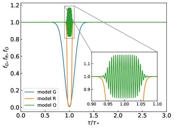
Figure 1: The non-minimal coupling $f(\tau/\tau_{*})$ in Eqs. (15), (16) and (17). Here we set $\Delta=0.1$, $\Lambda=0.01$, $\xi=0.001$ and the values of $A_{\text{G}}$, $A_{\text{R}}$ and $A_{\text{O}}$ are chosen for PBHs making up all of the CDM.

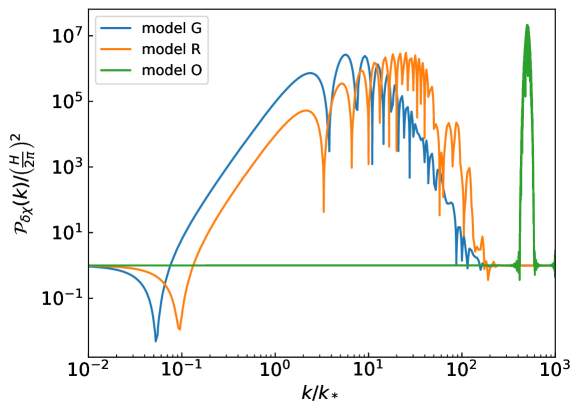
Figure 2: The power spectra of $\delta\chi$ for the three models corresponding to the features shown in Fig. 1.

III Formation of PBHs and scalar induced gravitational waves

The energy density of the spectator field is subdominant and therefore the perturbation of the spectator field does not contribute to the curvature perturbation during inflation. However, its perturbation can be converted into curvature perturbation at or after the end of inflation, such as in the model with nontrivial reheating field space surface Sasaki (2008); Huang (2009), modulated reheating model Suyama and Yamaguchi (2008); Dvali et al. (2004); Kofman (2003), curvaton mechanism Mollerach (1990); Linde and Mukhanov (1997); Enqvist and Sloth (2002); Lyth and Wands (2002); Moroi and Takahashi (2001); Sasaki et al. (2006); Enqvist and Nurmi (2005); Huang and Wang (2008); Huang (2008); Chingangbam and Huang (2009, 2011); Kawasaki et al. (2011) and so on, and may generate the local-type non-Gaussianity of curvature perturbation. Here we need to stress that the perturbativity condition Kristiano and Yokoyama (2022b); Meng et al. (2022) requires that such a curvature perturbation should be nearly Gaussian if the PBHs consist of most of the CDM in our Universe.

In this paper, we focus on the model in which the curvature perturbation is mainly produced by the spectator field. In the model with a nontrivial reheating surface in field space, the power spectrum of curvature perturbation generated by the spectator field is

$${\cal P}_{\zeta}=\cot^{2}\theta\left({{\cal H}\over\phi^{\prime}}\right)^{2}{\cal P}_{\delta\chi},$$ (22)

where $\theta$ is the angle between the reheating surface and the inflaton trajectory. In this scenario, the local-type non-Gaussianity is small as long as the reheating surface is a straight line Huang (2009). In the modulated reheating model, the decay rate of the inflaton field is related to the expectation value of $\chi$ by $\Gamma_{\phi}=\Gamma_{\phi}(\chi)$. The power spectrum of curvature perturbation is

$${\cal P}_{\zeta}=\alpha^{2}\left({\Gamma_{,\chi}\over\Gamma}\right)^{2}{\cal P}_{\delta\chi},$$ (23)

where $\alpha$ is a parameter depending on the ratio of $\Gamma$ to the Hubble parameter at the end of inflation. The local-type non-Gaussianity can be also small, for example, if the decay rate $\Gamma_{\phi}(\chi)$ linearly depends on $\chi$. In the curvaton scenario, for the curvaton field with quadratic potential, the curvaton linearly evolves after the end of inflation and then the poewer spectrum of curvature perturbation is

$${\cal P}_{\zeta}={4\over 9}{f_{D}^{2}\over\chi^{2}}{\cal P}_{\delta\chi},$$ (24)

where

$$f_{D}=\left.{3\rho_{\chi}\over 3\rho_{\chi}+4\rho_{R}}\right|_{t_{\text{decay}}},$$ (25)

$\rho_{\chi}$ and $\rho_{R}$ are the energy density of curvaton field and radiation at time of curvaton decay. In the curvaton model with quadratic potential, the non-Gaussianity parameter $f_{\text{NL}}$ is, Sasaki et al. (2006),

$$f_{\text{NL}}={5\over 4f_{D}}-{5\over 3}-{5f_{D}\over 6}.$$ (26)

The smallness of non-Gaussianity due to the perturbativity condition Meng et al. (2022) yields $f_{D}\simeq 1$, implying that the curvaton field becomes dominant when it decays.

The mass function of the PBHs at the formation time, $\beta(m_{\mathrm{pbh}})$, can be estimated using the Press-Schechter formalism Press and Schechter (1974), namely by integrating the probability distribution function (PDF) of the density contrast $P(\delta)$ over the region $\delta>\delta_{c}$,

$$\beta(m_{\mathrm{pbh}})=\int_{\delta_{c}}^{\infty}d\delta\frac{m_{\mathrm{pbh}}}{M_{H}}P(\delta),$$ (27)

where $\delta_{c}\sim 0.41$ is the critical value to form a single PBH Harada et al. (2013). The horizon mass $M_{H}$ is related to the comoving wavelength by

$$M_{H}\simeq 17\left(\frac{g}{10.75}\right)^{-1/6}\left(\frac{k}{10^{6}\mathrm{Mpc}^{-1}}\right)^{-2}M_{\odot},$$ (28)

and $g$ is the degress of freedom of relativistic particles at the formation time. The PDF, $P(\delta)$, takes the form of

$$P(\delta)=\frac{1}{\sqrt{2\pi\sigma_{k}^{2}}}\exp\left(-\frac{\delta^{2}}{2\sigma_{k}^{2}}\right),$$ (29)

with $\sigma_{k}^{2}(R)$ being smoothed variance of the density contrast on a comoving scale $R_{H}$:

$$\sigma_{k}^{2}=\left(\frac{4}{9}\right)^{2}\int_{0}^{\infty}\frac{dq}{q}W^{2}\left(q,R_{H}\right)\left(\frac{q}{k}\right)^{4}T^{2}\left(q,R_{H}\right)\mathcal{P}_{\zeta}(q).$$ (30)

Here, $W(k,R_{H})$ is the window function which we adopt a top-hat window function in real space, namely

$$W\left(k,R_{H}\right)=3\frac{\sin\left(kR_{H}\right)-\left(kR_{H}\right)\cos\left(kR_{H}\right)}{\left(kR_{H}\right)^{3}}.$$ (31)

$T(q,R_{H})$ denotes the transfer function during radiation dominated era which takes the form

$$T\left(k,R_{H}\right)=3\frac{\sin\left(kR_{H}/\sqrt{3}\right)-\left(kR_{H}/\sqrt{3}\right)\cos\left(kR_{H}/\sqrt{3}\right)}{\left(kR_{H}/\sqrt{3}\right)^{3}}$$ (32)

The mass of PBH in Eq. (27) is realted to $\delta$ by $m_{\mathrm{pbh}}=M_{H}\kappa\left(\delta_{m}-\delta_{c}\right)^{\gamma}$ Choptuik (1993); Evans and Coleman (1994); Niemeyer and Jedamzik (1998), where $\kappa=3.3$, $\gamma=0.36$ Koike et al. (1995) and $\delta_{m}=\delta-3/8\delta^{2}$ accounts for nonlinear effects Young et al. (2019); De Luca et al. (2019a); Kawasaki and Nakatsuka (2019). The relation between the fraction of PBHs in the CDM at present, $f_{\mathrm{pbh}}(m_{\mathrm{pbh}})$, and $\beta(m_{\mathrm{pbh}})$ can be written as

$$f_{\mathrm{pbh}}(m_{\mathrm{pbh}})=\frac{1}{\Omega_{\mathrm{CDM}}}\left(\frac{M_{\mathrm{eq}}}{m_{\mathrm{pbh}}}\right)^{1/2}\beta(m_{\mathrm{pbh}}),$$ (33)

where we use the convention such that $f_{\mathrm{pbh}}\equiv{\Omega_{\mathrm{PBH}}/\Omega_{\mathrm{CDM}}}=\int f_{\mathrm{pbh}}(m_{\mathrm{pbh}})\mathrm{d}\ln m_{\mathrm{pbh}}$ and $M_{\mathrm{eq}}=2.8\times 10^{17}M_{\odot}$. The numeric results of $f_{\mathrm{pbh}}(m_{\mathrm{pbh}})$ are shown in Fig. 3. Although various independent constraints on $f_{\mathrm{pbh}}$ have excluded PBHs in the mass range $\sim[10^{-18},10^{3}]M_{\odot}$ to a percent level, PBHs are still able to represent all the CDM within $\sim[10^{-16},10^{-14}]M_{\odot}$ and $\sim[10^{-13},10^{-12}]M_{\odot}$. We choose $k_{*}=7\times 10^{11}\mathrm{Mpc^{-1}}$, $k_{*}=2\times 10^{11}\mathrm{Mpc^{-1}}$ and $k_{*}=9\times 10^{9}\mathrm{Mpc^{-1}}$ in model G, model R and model O respectively, and then all these models can generate sufficient PBHs peaked at $\sim 10^{-12}M_{\odot}$ that can represent all the CDM. It can be seen that the $f_{\mathrm{pbh}}(m_{\mathrm{pbh}})$ for these three models are all compatible with current observational constraints.

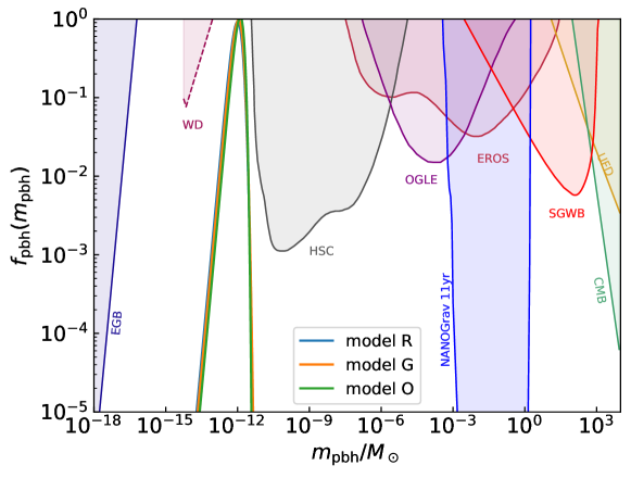
Figure 3: The fraction of PBHs, $f_{\mathrm{pbh}}(m_{\mathrm{pbh}})$, for the three models corresponding to the features shown in Fig. 1. Here the PBHs make up all of the CDM. We also plot an overview of the current observational constraints on $f_{\mathrm{pbh}}$, including extra-galactic Gamma-ray background (EGB) Carr et al. (2010), white dwarfs (WD) Graham et al. (2015) (note that this constraint might be relaxed, see Montero-Camacho et al. (2019)), Subaru/HSC Niikura et al. (2019a), EROS/MACHO Tisserand et al. (2007), OGLE Niikura et al. (2019b), stochastic gravitational wave background (SGWB) from binary PBHs Wang et al. (2018); Chen and Huang (2020), ultra-faint dwarf galaxies (UFD) Brandt (2016) and NANOGrav Chen et al. (2020a).

In addition, the linear scalar perturbations would source second-order tensor perturbations during the radiation dominated era, also dubbed as SIGWs Tomita (1967); Matarrese et al. (1993, 1994, 1998); Noh and Hwang (2004); Carbone and Matarrese (2005); Nakamura (2007). SIGWs were inevitably generated during the formation of PBHs and can be a powerful tool to search or constrain PBHs Ananda et al. (2007); Baumann et al. (2007); Saito and Yokoyama (2009); Arroja et al. (2009); Assadullahi and Wands (2010); Bugaev and Klimai (2010a, b); Saito and Yokoyama (2010); Bugaev and Klimai (2011); Alabidi et al. (2013); Nakama and Suyama (2016); Nakama et al. (2017); Inomata et al. (2017b); Orlofsky et al. (2017); Garcia-Bellido et al. (2017); Sasaki et al. (2018); Espinosa et al. (2018b); Kohri and Terada (2018); Cai et al. (2019b); Bartolo et al. (2019a, b); Unal (2019); Byrnes et al. (2019); Inomata and Nakama (2019); Clesse et al. (2018); Cai et al. (2019c); Inomata et al. (2019a, b); Cai et al. (2019d); Yuan et al. (2019a); Cai et al. (2019e); Lu et al. (2019); Yuan et al. (2019b); Tomikawa and Kobayashi (2019); De Luca et al. (2019b); Yuan et al. (2020); Inomata et al. (2020a, b, c); Yuan and Huang (2020); Papanikolaou et al. (2020); Zhang et al. (2020a); Kapadia et al. (2020); Zhang et al. (2020b); Domènech et al. (2020); Dalianis and Kouvaris (2020); Atal and Domènech (2021); Chen et al. (2022); Franciolini (2021); Witkowski et al. (2022); Balaji et al. (2022); Cang et al. (2022); Gehrman et al. (2022); Braglia et al. (2021); Papanikolaou (2022). For review of SIGW, see Yuan and Huang (2021); Domènech (2021). The superposition of SIGWs all over the sky will form a stochastic gravitational wave background whose energy spectrum is defined as the energy of GWs per logarithm frequency normalized by the critical energy. The energy spectrum of SIGWs at equality time can be evaluated semi-analytically as Kohri and Terada (2018)

$$\Omega_{\mathrm{GW}}(k)=\frac{1}{6}\int_{0}^{\infty}\mathrm{d}u\int_{|1-u|}^{1+u}\mathrm{~{}d}v\frac{v^{2}}{u^{2}}\left[1-\left(\frac{1+v^{2}-u^{2}}{2v}\right)^{2}\right]^{2}\mathcal{P}_{\zeta}(uk)\mathcal{P}_{\zeta}(vk)\overline{I^{2}(u,v,x\rightarrow\infty)},$$ (34)

where the oscillating average of the square of the kernel function in the sub-horizon limit is given by Kohri and Terada (2018)

$$\overline{I^{2}}=\frac{9\left(u^{2}+v^{2}-3\right)^{2}}{32u^{6}v^{6}}\Bigg{\{}\left[-4uv+\left(u^{2}+v^{2}-3\right)\ln\left|\frac{3-(u+v)^{2}}{3-(u-v)^{2}}\right|\right]^{2}+\pi^{2}\left(u^{2}+v^{2}-3\right)^{2}\Theta(u+v-\sqrt{3})\Bigg{\}}.$$ (35)

The energy spectrum of SGIWs at present, $\Omega_{\mathrm{GW,0}}(k)$, is evaluated by $\Omega_{\mathrm{GW,0}}(k)=\Omega_{r}\Omega_{\mathrm{GW}}(k)$, where $\Omega_{r}$ is the density parameter of radiation by today. The results of $\Omega_{\mathrm{GW,0}}(f)$ are shown in Fig. 4.

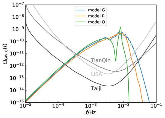
Figure 4: The energy spectrum of SIGWs for the three models corresponding to the features shown in Fig. 1. Here black, dark grey and light grey curves correspond to the power-law integrated sensitivity curves for Taiji Hu and Wu (2017), TianQin Luo et al. (2016) and LISA Audley et al. (2017) respectively, assuming a four year detection.

Here, the wavelength $k$ is realted to the frequency by $k=2\pi f$ in the $c=1$ unit. It can be seen that the SIGWs accompanying the formation of $\sim 10^{-12}M_{\odot}$ PBHs generated by model G, model R and model O can be detected by the future space-borne GW detectors such as Taiji Hu and Wu (2017), TianQin Luo et al. (2016) and LISA Audley et al. (2017).

IV Summary and Discussion

In this paper, we improve and generalize the non-minimal curvaton model with a sharp dip Pi and Sasaki (2021) to a more general non-minimal spectator model for the formation of PBHs. Since the coupling between the inflaton and spectator fields is supposed to have a sharp feature controlled by the expectation value of the inflaton field, the power spectrum of the perturbation of the spectator field for some perturbation modes stretching outside the horizon when the inflaton field rolls in the region of the feature are significantly amplified. At or after the end of inflation, the perturbation of the spectator field is converted into the curvature perturbation and the enhanced curvature perturbation at small scales due to the feature in the coupling between spectator and inflaton fields leads to the formation of PBHs. Our model can produce a sizeable amount of PBHs peaked at $\sim 10^{-12}M_{\odot}$ for consisting of all the CDM and the SIGWs can be detected by future space-borne GW detectors such as Taiji, TianQin and LISA.

Acknowledgments. This work is supported by the National Key Research and Development Program of China Grant No.2020YFC2201502, grants from NSFC (grant No. 11975019, 11991052, 12047503), Key Research Program of Frontier Sciences, CAS, Grant NO. ZDBS-LY-7009, CAS Project for Young Scientists in Basic Research YSBR-006, the Key Research Program of the Chinese Academy of Sciences (Grant NO. XDPB15). We acknowledge the use of HPC Cluster of ITP-CAS and GWSC.jl package (https://github.com/bingining/gwsc.jl) for plotting the power-law integrated sensitivity curves of Taiji, TianQin and LISA.

References

- Zel’dovich and Novikov (1967) Ya. B. Zel’dovich and I. D. Novikov, “The Hypothesis of Cores Retarded during Expansion and the Hot Cosmological Model,” Soviet Astron. AJ (Engl. Transl. ), 10, 602 (1967).
- Hawking (1971) Stephen Hawking, “Gravitationally collapsed objects of very low mass,” Mon. Not. Roy. Astron. Soc. 152, 75 (1971).
- Carr and Hawking (1974) Bernard J. Carr and S. W. Hawking, “Black holes in the early Universe,” Mon. Not. Roy. Astron. Soc. 168, 399–415 (1974).
- Carr (1975) Bernard J. Carr, “The Primordial black hole mass spectrum,” Astrophys. J. 201, 1–19 (1975).
- Bird et al. (2016) Simeon Bird, Ilias Cholis, Julian B. Muñoz, Yacine Ali-Haïmoud, Marc Kamionkowski, Ely D. Kovetz, Alvise Raccanelli, and Adam G. Riess, “Did LIGO detect dark matter?” Phys. Rev. Lett. 116, 201301 (2016), arXiv:1603.00464 [astro-ph.CO] .
- Sasaki et al. (2016) Misao Sasaki, Teruaki Suyama, Takahiro Tanaka, and Shuichiro Yokoyama, “Primordial Black Hole Scenario for the Gravitational-Wave Event GW150914,” Phys. Rev. Lett. 117, 061101 (2016), [Erratum: Phys.Rev.Lett. 121, 059901 (2018)], arXiv:1603.08338 [astro-ph.CO] .
- Clesse and García-Bellido (2017) Sebastien Clesse and Juan García-Bellido, “The clustering of massive Primordial Black Holes as Dark Matter: measuring their mass distribution with Advanced LIGO,” Phys. Dark Univ. 15, 142–147 (2017), arXiv:1603.05234 [astro-ph.CO] .
- Wang et al. (2018) Sai Wang, Yi-Fan Wang, Qing-Guo Huang, and Tjonnie G. F. Li, “Constraints on the Primordial Black Hole Abundance from the First Advanced LIGO Observation Run Using the Stochastic Gravitational-Wave Background,” Phys. Rev. Lett. 120, 191102 (2018), arXiv:1610.08725 [astro-ph.CO] .
- Ali-Haïmoud et al. (2017) Yacine Ali-Haïmoud, Ely D. Kovetz, and Marc Kamionkowski, “Merger rate of primordial black-hole binaries,” Phys. Rev. D96, 123523 (2017), arXiv:1709.06576 [astro-ph.CO] .
- Chen and Huang (2018) Zu-Cheng Chen and Qing-Guo Huang, “Merger Rate Distribution of Primordial-Black-Hole Binaries,” Astrophys. J. 864, 61 (2018), arXiv:1801.10327 [astro-ph.CO] .
- Chen et al. (2019) Zu-Cheng Chen, Fan Huang, and Qing-Guo Huang, “Stochastic Gravitational-wave Background from Binary Black Holes and Binary Neutron Stars and Implications for LISA,” Astrophys. J. 871, 97 (2019), arXiv:1809.10360 [gr-qc] .
- Kavanagh et al. (2018) Bradley J. Kavanagh, Daniele Gaggero, and Gianfranco Bertone, “Merger rate of a subdominant population of primordial black holes,” Phys. Rev. D98, 023536 (2018), arXiv:1805.09034 [astro-ph.CO] .
- Raidal et al. (2019) Martti Raidal, Christian Spethmann, Ville Vaskonen, and Hardi Veermäe, “Formation and Evolution of Primordial Black Hole Binaries in the Early Universe,” JCAP 1902, 018 (2019), arXiv:1812.01930 [astro-ph.CO] .
- Liu et al. (2019a) Lang Liu, Zong-Kuan Guo, and Rong-Gen Cai, “Effects of the surrounding primordial black holes on the merger rate of primordial black hole binaries,” Phys. Rev. D99, 063523 (2019a), arXiv:1812.05376 [astro-ph.CO] .
- Chen and Huang (2020) Zu-Cheng Chen and Qing-Guo Huang, “Distinguishing Primordial Black Holes from Astrophysical Black Holes by Einstein Telescope and Cosmic Explorer,” JCAP 08, 039 (2020), arXiv:1904.02396 [astro-ph.CO] .
- Yuan et al. (2019a) Chen Yuan, Zu-Cheng Chen, and Qing-Guo Huang, “Probing Primordial-Black-Hole Dark Matter with Scalar Induced Gravitational Waves,” Phys. Rev. D100, 081301 (2019a), arXiv:1906.11549 [astro-ph.CO] .
- Liu et al. (2019b) Lang Liu, Zong-Kuan Guo, and Rong-Gen Cai, “Effects of the merger history on the merger rate density of primordial black hole binaries,” (2019b), arXiv:1901.07672 [astro-ph.CO] .
- De Luca et al. (2021) V. De Luca, V. Desjacques, G. Franciolini, P. Pani, and A. Riotto, “GW190521 Mass Gap Event and the Primordial Black Hole Scenario,” Phys. Rev. Lett. 126, 051101 (2021), arXiv:2009.01728 [astro-ph.CO] .
- Vattis et al. (2020) Kyriakos Vattis, Isabelle S. Goldstein, and Savvas M. Koushiappas, “Could the 2.6 object in GW190814 be a primordial black hole?” Phys. Rev. D 102, 061301 (2020), arXiv:2006.15675 [astro-ph.HE] .
- Wang and Zhao (2022) Sai Wang and Zhi-Chao Zhao, “GW200105 and GW200115 are compatible with a scenario of primordial black hole binary coalescences,” Eur. Phys. J. C 82, 9 (2022), arXiv:2107.00450 [astro-ph.CO] .
- Chen et al. (2022) Zu-Cheng Chen, Chen Yuan, and Qing-Guo Huang, “Confronting the primordial black hole scenario with the gravitational-wave events detected by LIGO-Virgo,” Phys. Lett. B 829, 137040 (2022), arXiv:2108.11740 [astro-ph.CO] .
- Abbott et al. (2016) B. P. Abbott et al. (LIGO Scientific, Virgo), “Binary Black Hole Mergers in the first Advanced LIGO Observing Run,” Phys. Rev. X 6, 041015 (2016), [Erratum: Phys.Rev.X 8, 039903 (2018)], arXiv:1606.04856 [gr-qc] .
- Abbott et al. (2021) R. Abbott et al. (LIGO Scientific, VIRGO, KAGRA), “GWTC-3: Compact Binary Coalescences Observed by LIGO and Virgo During the Second Part of the Third Observing Run,” (2021), arXiv:2111.03606 [gr-qc] .
- Carr et al. (2010) B. J. Carr, Kazunori Kohri, Yuuiti Sendouda, and Jun’ichi Yokoyama, “New cosmological constraints on primordial black holes,” Phys. Rev. D 81, 104019 (2010), arXiv:0912.5297 [astro-ph.CO] .
- Graham et al. (2015) Peter W. Graham, Surjeet Rajendran, and Jaime Varela, “Dark Matter Triggers of Supernovae,” Phys. Rev. D 92, 063007 (2015), arXiv:1505.04444 [hep-ph] .
- Niikura et al. (2019a) Hiroko Niikura et al., “Microlensing constraints on primordial black holes with Subaru/HSC Andromeda observations,” Nature Astron. 3, 524–534 (2019a), arXiv:1701.02151 [astro-ph.CO] .
- Tisserand et al. (2007) P. Tisserand et al. (EROS-2), “Limits on the Macho Content of the Galactic Halo from the EROS-2 Survey of the Magellanic Clouds,” Astron. Astrophys. 469, 387–404 (2007), arXiv:astro-ph/0607207 .
- Niikura et al. (2019b) Hiroko Niikura, Masahiro Takada, Shuichiro Yokoyama, Takahiro Sumi, and Shogo Masaki, “Constraints on Earth-mass primordial black holes from OGLE 5-year microlensing events,” Phys. Rev. D 99, 083503 (2019b), arXiv:1901.07120 [astro-ph.CO] .
- Brandt (2016) Timothy D. Brandt, “Constraints on MACHO Dark Matter from Compact Stellar Systems in Ultra-Faint Dwarf Galaxies,” Astrophys. J. Lett. 824, L31 (2016), arXiv:1605.03665 [astro-ph.GA] .
- Chen et al. (2020a) Zu-Cheng Chen, Chen Yuan, and Qing-Guo Huang, “Pulsar Timing Array Constraints on Primordial Black Holes with NANOGrav 11-Year Dataset,” Phys. Rev. Lett. 124, 251101 (2020a), arXiv:1910.12239 [astro-ph.CO] .
- Montero-Camacho et al. (2019) Paulo Montero-Camacho, Xiao Fang, Gabriel Vasquez, Makana Silva, and Christopher M. Hirata, “Revisiting constraints on asteroid-mass primordial black holes as dark matter candidates,” JCAP 08, 031 (2019), arXiv:1906.05950 [astro-ph.CO] .
- Laha (2019) Ranjan Laha, “Primordial Black Holes as a Dark Matter Candidate Are Severely Constrained by the Galactic Center 511 keV -Ray Line,” Phys. Rev. Lett. 123, 251101 (2019), arXiv:1906.09994 [astro-ph.HE] .
- Dasgupta et al. (2020) Basudeb Dasgupta, Ranjan Laha, and Anupam Ray, “Neutrino and positron constraints on spinning primordial black hole dark matter,” Phys. Rev. Lett. 125, 101101 (2020), arXiv:1912.01014 [hep-ph] .
- Laha et al. (2020) Ranjan Laha, Julian B. Muñoz, and Tracy R. Slatyer, “INTEGRAL constraints on primordial black holes and particle dark matter,” Phys. Rev. D 101, 123514 (2020), arXiv:2004.00627 [astro-ph.CO] .
- Saha and Laha (2022) Akash Kumar Saha and Ranjan Laha, “Sensitivities on nonspinning and spinning primordial black hole dark matter with global 21-cm troughs,” Phys. Rev. D 105, 103026 (2022), arXiv:2112.10794 [astro-ph.CO] .
- Ray et al. (2021) Anupam Ray, Ranjan Laha, Julian B. Muñoz, and Regina Caputo, “Near future MeV telescopes can discover asteroid-mass primordial black hole dark matter,” Phys. Rev. D 104, 023516 (2021), arXiv:2102.06714 [astro-ph.CO] .
- Carr et al. (2020) Bernard Carr, Kazunori Kohri, Yuuiti Sendouda, and Jun’ichi Yokoyama, “Constraints on Primordial Black Holes,” (2020), arXiv:2002.12778 [astro-ph.CO] .
- Escrivà et al. (2022) Albert Escrivà, Florian Kuhnel, and Yuichiro Tada, “Primordial Black Holes,” (2022), arXiv:2211.05767 [astro-ph.CO] .
- Aghanim et al. (2020) N. Aghanim et al. (Planck), “Planck 2018 results. VI. Cosmological parameters,” Astron. Astrophys. 641, A6 (2020), [Erratum: Astron.Astrophys. 652, C4 (2021)], arXiv:1807.06209 [astro-ph.CO] .
- Yokoyama (1998) Jun’ichi Yokoyama, “Chaotic new inflation and formation of primordial black holes,” Phys. Rev. D 58, 083510 (1998), arXiv:astro-ph/9802357 .
- Kinney (2005) William H. Kinney, “Horizon crossing and inflation with large eta,” Phys. Rev. D 72, 023515 (2005), arXiv:gr-qc/0503017 .
- Choudhury and Mazumdar (2014) Sayantan Choudhury and Anupam Mazumdar, “Primordial blackholes and gravitational waves for an inflection-point model of inflation,” Phys. Lett. B 733, 270–275 (2014), arXiv:1307.5119 [astro-ph.CO] .
- Garcia-Bellido et al. (2016) Juan Garcia-Bellido, Marco Peloso, and Caner Unal, “Gravitational waves at interferometer scales and primordial black holes in axion inflation,” JCAP 12, 031 (2016), arXiv:1610.03763 [astro-ph.CO] .
- Cheng et al. (2017) Shu-Lin Cheng, Wolung Lee, and Kin-Wang Ng, “Production of high stellar-mass primordial black holes in trapped inflation,” JHEP 02, 008 (2017), arXiv:1606.00206 [astro-ph.CO] .
- Garcia-Bellido and Ruiz Morales (2017) Juan Garcia-Bellido and Ester Ruiz Morales, “Primordial black holes from single field models of inflation,” Phys. Dark Univ. 18, 47–54 (2017), arXiv:1702.03901 [astro-ph.CO] .
- Cheng et al. (2018) Shu-Lin Cheng, Wolung Lee, and Kin-Wang Ng, “Primordial black holes and associated gravitational waves in axion monodromy inflation,” JCAP 07, 001 (2018), arXiv:1801.09050 [astro-ph.CO] .
- Dalianis et al. (2019) Ioannis Dalianis, Alex Kehagias, and George Tringas, “Primordial black holes from -attractors,” JCAP 01, 037 (2019), arXiv:1805.09483 [astro-ph.CO] .
- Tada and Yokoyama (2019) Yuichiro Tada and Shuichiro Yokoyama, “Primordial black hole tower: Dark matter, earth-mass, and LIGO black holes,” Phys. Rev. D 100, 023537 (2019), arXiv:1904.10298 [astro-ph.CO] .
- Xu et al. (2020) Wu-Tao Xu, Jing Liu, Tie-Jun Gao, and Zong-Kuan Guo, “Gravitational waves from double-inflection-point inflation,” Phys. Rev. D 101, 023505 (2020), arXiv:1907.05213 [astro-ph.CO] .
- Mishra and Sahni (2020) Swagat S. Mishra and Varun Sahni, “Primordial Black Holes from a tiny bump/dip in the Inflaton potential,” JCAP 04, 007 (2020), arXiv:1911.00057 [gr-qc] .
- Bhaumik and Jain (2020) Nilanjandev Bhaumik and Rajeev Kumar Jain, “Primordial black holes dark matter from inflection point models of inflation and the effects of reheating,” JCAP 01, 037 (2020), arXiv:1907.04125 [astro-ph.CO] .
- Liu et al. (2020) Jing Liu, Zong-Kuan Guo, and Rong-Gen Cai, “Analytical approximation of the scalar spectrum in the ultraslow-roll inflationary models,” Phys. Rev. D 101, 083535 (2020), arXiv:2003.02075 [astro-ph.CO] .
- Atal et al. (2020) Vicente Atal, Judith Cid, Albert Escrivà, and Jaume Garriga, “PBH in single field inflation: the effect of shape dispersion and non-Gaussianities,” JCAP 05, 022 (2020), arXiv:1908.11357 [astro-ph.CO] .
- Fu et al. (2020) Chengjie Fu, Puxun Wu, and Hongwei Yu, “Primordial black holes and oscillating gravitational waves in slow-roll and slow-climb inflation with an intermediate noninflationary phase,” Phys. Rev. D 102, 043527 (2020), arXiv:2006.03768 [astro-ph.CO] .
- Vennin (2020) Vincent Vennin, Stochastic inflation and primordial black holes, Other thesis (2020), arXiv:2009.08715 [astro-ph.CO] .
- Ragavendra et al. (2020) H. V. Ragavendra, Pankaj Saha, L. Sriramkumar, and Joseph Silk, “PBHs and secondary GWs from ultra slow roll and punctuated inflation,” (2020), arXiv:2008.12202 [astro-ph.CO] .
- Gao and Yang (2021) Tie-Jun Gao and Xiu-Yi Yang, “Double peaks of gravitational wave spectrum induced from inflection point inflation,” Eur. Phys. J. C 81, 494 (2021), arXiv:2101.07616 [astro-ph.CO] .
- Cai et al. (2022) Yi-Fu Cai, Xiao-Han Ma, Misao Sasaki, Dong-Gang Wang, and Zihan Zhou, “Highly non-Gaussian tails and primordial black holes from single-field inflation,” (2022), arXiv:2207.11910 [astro-ph.CO] .
- Karam et al. (2022) Alexandros Karam, Niko Koivunen, Eemeli Tomberg, Ville Vaskonen, and Hardi Veermäe, “Anatomy of single-field inflationary models for primordial black holes,” (2022), arXiv:2205.13540 [astro-ph.CO] .
- Di and Gong (2018) Haoran Di and Yungui Gong, “Primordial black holes and second order gravitational waves from ultra-slow-roll inflation,” JCAP 07, 007 (2018), arXiv:1707.09578 [astro-ph.CO] .
- Cai et al. (2018) Yi-Fu Cai, Xi Tong, Dong-Gang Wang, and Sheng-Feng Yan, “Primordial Black Holes from Sound Speed Resonance during Inflation,” Phys. Rev. Lett. 121, 081306 (2018), arXiv:1805.03639 [astro-ph.CO] .
- Chen et al. (2020b) Chao Chen, Xiao-Han Ma, and Yi-Fu Cai, “Dirac-Born-Infeld realization of sound speed resonance mechanism for primordial black holes,” Phys. Rev. D 102, 063526 (2020b), arXiv:2003.03821 [astro-ph.CO] .
- Cai et al. (2019a) Yi-Fu Cai, Chao Chen, Xi Tong, Dong-Gang Wang, and Sheng-Feng Yan, “When Primordial Black Holes from Sound Speed Resonance Meet a Stochastic Background of Gravitational Waves,” Phys. Rev. D 100, 043518 (2019a), arXiv:1902.08187 [astro-ph.CO] .
- Cai et al. (2020) Rong-Gen Cai, Zong-Kuan Guo, Jing Liu, Lang Liu, and Xing-Yu Yang, “Primordial black holes and gravitational waves from parametric amplification of curvature perturbations,” JCAP 06, 013 (2020), arXiv:1912.10437 [astro-ph.CO] .
- Cotner and Kusenko (2017a) Eric Cotner and Alexander Kusenko, “Primordial black holes from supersymmetry in the early universe,” Phys. Rev. Lett. 119, 031103 (2017a), arXiv:1612.02529 [astro-ph.CO] .
- Cotner and Kusenko (2017b) Eric Cotner and Alexander Kusenko, “Primordial black holes from scalar field evolution in the early universe,” Phys. Rev. D 96, 103002 (2017b), arXiv:1706.09003 [astro-ph.CO] .
- Cotner et al. (2018) Eric Cotner, Alexander Kusenko, and Volodymyr Takhistov, “Primordial Black Holes from Inflaton Fragmentation into Oscillons,” Phys. Rev. D 98, 083513 (2018), arXiv:1801.03321 [astro-ph.CO] .
- Cotner et al. (2019) Eric Cotner, Alexander Kusenko, Misao Sasaki, and Volodymyr Takhistov, “Analytic Description of Primordial Black Hole Formation from Scalar Field Fragmentation,” JCAP 10, 077 (2019), arXiv:1907.10613 [astro-ph.CO] .
- Escrivà and Subils (2022) Albert Escrivà and Javier G. Subils, “Primordial Black Hole Formation during a Strongly Coupled Crossover,” (2022), arXiv:2211.15674 [astro-ph.CO] .
- Pi and Wang (2022) Shi Pi and Jianing Wang, “Primordial Black Hole Formation in Starobinsky’s Linear Potential Model,” (2022), arXiv:2209.14183 [astro-ph.CO] .
- Germani and Prokopec (2017) Cristiano Germani and Tomislav Prokopec, “On primordial black holes from an inflection point,” Phys. Dark Univ. 18, 6–10 (2017), arXiv:1706.04226 [astro-ph.CO] .
- Byrnes et al. (2019) Christian T. Byrnes, Philippa S. Cole, and Subodh P. Patil, “Steepest growth of the power spectrum and primordial black holes,” JCAP 06, 028 (2019), arXiv:1811.11158 [astro-ph.CO] .
- Passaglia et al. (2019) Samuel Passaglia, Wayne Hu, and Hayato Motohashi, “Primordial black holes and local non-Gaussianity in canonical inflation,” Phys. Rev. D 99, 043536 (2019), arXiv:1812.08243 [astro-ph.CO] .
- Fu et al. (2019a) Chengjie Fu, Puxun Wu, and Hongwei Yu, “Primordial Black Holes from Inflation with Nonminimal Derivative Coupling,” Phys. Rev. D 100, 063532 (2019a), arXiv:1907.05042 [astro-ph.CO] .
- Fu et al. (2019b) Chengjie Fu, Puxun Wu, and Hongwei Yu, “Scalar induced gravitational waves in inflation with gravitationally enhanced friction,” (2019b), arXiv:1912.05927 [astro-ph.CO] .
- Inomata et al. (2022a) Keisuke Inomata, Evan McDonough, and Wayne Hu, “Amplification of primordial perturbations from the rise or fall of the inflaton,” JCAP 02, 031 (2022a), arXiv:2110.14641 [astro-ph.CO] .
- Tasinato (2021) Gianmassimo Tasinato, “An analytic approach to non-slow-roll inflation,” Phys. Rev. D 103, 023535 (2021), arXiv:2012.02518 [hep-th] .
- Cole et al. (2022) Philippa S. Cole, Andrew D. Gow, Christian T. Byrnes, and Subodh P. Patil, “Steepest growth re-examined: repercussions for primordial black hole formation,” (2022), arXiv:2204.07573 [astro-ph.CO] .
- Fu and Wang (2022) Chengjie Fu and Shao-Jiang Wang, “Primordial black holes and induced gravitational waves from double-pole inflation,” (2022), arXiv:2211.03523 [astro-ph.CO] .
- Peng et al. (2021) Zhi-Zhang Peng, Chengjie Fu, Jing Liu, Zong-Kuan Guo, and Rong-Gen Cai, “Gravitational waves from resonant amplification of curvature perturbations during inflation,” JCAP 10, 050 (2021), arXiv:2106.11816 [astro-ph.CO] .
- Zhai et al. (2022) Rongrong Zhai, Hongwei Yu, and Puxun Wu, “Growth of power spectrum due to decrease of sound speed during inflation,” Phys. Rev. D 106, 023517 (2022), arXiv:2207.12745 [gr-qc] .
- Kannike et al. (2017) Kristjan Kannike, Luca Marzola, Martti Raidal, and Hardi Veermäe, “Single Field Double Inflation and Primordial Black Holes,” JCAP 09, 020 (2017), arXiv:1705.06225 [astro-ph.CO] .
- Gao and Guo (2018) Tie-Jun Gao and Zong-Kuan Guo, “Primordial Black Hole Production in Inflationary Models of Supergravity with a Single Chiral Superfield,” Phys. Rev. D 98, 063526 (2018), arXiv:1806.09320 [hep-ph] .
- Cheong et al. (2021) Dhong Yeon Cheong, Sung Mook Lee, and Seong Chan Park, “Primordial black holes in Higgs- inflation as the whole of dark matter,” JCAP 01, 032 (2021), arXiv:1912.12032 [hep-ph] .
- Cheong et al. (2020) Dhong Yeon Cheong, Hyun Min Lee, and Seong Chan Park, “Beyond the Starobinsky model for inflation,” Phys. Lett. B 805, 135453 (2020), arXiv:2002.07981 [hep-ph] .
- Dalianis et al. (2020) Ioannis Dalianis, Stelios Karydas, and Eleftherios Papantonopoulos, “Generalized Non-Minimal Derivative Coupling: Application to Inflation and Primordial Black Hole Production,” JCAP 06, 040 (2020), arXiv:1910.00622 [astro-ph.CO] .
- Martin et al. (2020a) Jérôme Martin, Theodoros Papanikolaou, and Vincent Vennin, “Primordial black holes from the preheating instability in single-field inflation,” JCAP 01, 024 (2020a), arXiv:1907.04236 [astro-ph.CO] .
- Martin et al. (2020b) Jérôme Martin, Theodoros Papanikolaou, Lucas Pinol, and Vincent Vennin, “Metric preheating and radiative decay in single-field inflation,” JCAP 05, 003 (2020b), arXiv:2002.01820 [astro-ph.CO] .
- Lin et al. (2020) Jiong Lin, Qing Gao, Yungui Gong, Yizhou Lu, Chao Zhang, and Fengge Zhang, “Primordial black holes and secondary gravitational waves from and inflation,” Phys. Rev. D 101, 103515 (2020), arXiv:2001.05909 [gr-qc] .
- Yi et al. (2020) Zhu Yi, Qing Gao, Yungui Gong, and Zong-hong Zhu, “Primordial black holes and secondary gravitational waves from inflationary model with a non-canonical kinetic term,” (2020), arXiv:2011.10606 [astro-ph.CO] .
- Gao et al. (2020) Qing Gao, Yungui Gong, and Zhu Yi, “Primordial black holes and secondary gravitational waves from natural inflation,” (2020), arXiv:2012.03856 [gr-qc] .
- Gao (2021) Qing Gao, “Primordial black holes and secondary gravitational waves from chaotic inflation,” (2021), arXiv:2102.07369 [gr-qc] .
- Wu et al. (2021) Lina Wu, Yungui Gong, and Tianjun Li, “Primordial black holes and secondary gravitational waves from string inspired general no-scale supergravity,” Phys. Rev. D 104, 123544 (2021), arXiv:2105.07694 [gr-qc] .
- Teimoori et al. (2021) Zeinab Teimoori, Kazem Rezazadeh, and Kayoomars Karami, “Primordial Black Holes Formation and Secondary Gravitational Waves in Nonminimal Derivative Coupling Inflation,” Astrophys. J. 915, 118 (2021), arXiv:2107.08048 [gr-qc] .
- Kawai and Kim (2021) Shinsuke Kawai and Jinsu Kim, “Primordial black holes from Gauss-Bonnet-corrected single field inflation,” Phys. Rev. D 104, 083545 (2021), arXiv:2108.01340 [astro-ph.CO] .
- Zhang (2022) Fengge Zhang, “Primordial black holes and scalar induced gravitational waves from the E model with a Gauss-Bonnet term,” Phys. Rev. D 105, 063539 (2022), arXiv:2112.10516 [gr-qc] .
- Yi (2022) Zhu Yi, “Primordial black holes and scalar-induced gravitational waves from scalar-tensor inflation,” (2022), arXiv:2206.01039 [gr-qc] .
- Gu et al. (2022) Bao-Min Gu, Fu-Wen Shu, Ke Yang, and Yu-Peng Zhang, “Primordial black holes from valley,” (2022), arXiv:2207.09968 [astro-ph.CO] .
- Cook (2022) Jessica L. Cook, “Primordial Black Hole Production in Natural and Hilltop Inflation,” (2022), arXiv:2209.05674 [astro-ph.CO] .
- Hidalgo et al. (2022) Juan Carlos Hidalgo, Luis E. Padilla, and Gabriel German, “Production of PBHs from inflaton structure,” (2022), arXiv:2208.09462 [astro-ph.CO] .
- Animali and Vennin (2022) Chiara Animali and Vincent Vennin, “Primordial black holes from stochastic tunnelling,” (2022), arXiv:2210.03812 [astro-ph.CO] .
- Papanikolaou et al. (2022) Theodoros Papanikolaou, Andreas Lymperis, Smaragda Lola, and Emmanuel N. Saridakis, “Primordial black holes and gravitational waves from non-canonical inflation,” (2022), arXiv:2211.14900 [astro-ph.CO] .
- Braglia et al. (2022) Matteo Braglia, Andrei Linde, Renata Kallosh, and Fabio Finelli, “Hybrid -attractors, primordial black holes and gravitational wave backgrounds,” (2022), arXiv:2211.14262 [astro-ph.CO] .
- Kawaguchi and Tsujikawa (2022) Ryodai Kawaguchi and Shinji Tsujikawa, “Primordial black holes from Higgs inflation with a Gauss-Bonnet coupling,” (2022), arXiv:2211.13364 [astro-ph.CO] .
- Ashoorioon et al. (2021a) Amjad Ashoorioon, Abasalt Rostami, and Javad T. Firouzjaee, “EFT compatible PBHs: effective spawning of the seeds for primordial black holes during inflation,” JHEP 07, 087 (2021a), arXiv:1912.13326 [astro-ph.CO] .
- Fu and Chen (2022) Chengjie Fu and Chao Chen, “Sudden braking and turning in the single/multi-stream inflation: primordial black hole formation,” (2022), arXiv:2211.11387 [astro-ph.CO] .
- Ahmed et al. (2022) Waqas Ahmed, M. Junaid, and Umer Zubair, “Primordial black holes and gravitational waves in hybrid inflation with chaotic potentials,” Nucl. Phys. B 984, 115968 (2022), arXiv:2109.14838 [astro-ph.CO] .
- Garcia-Bellido et al. (1996) Juan Garcia-Bellido, Andrei D. Linde, and David Wands, “Density perturbations and black hole formation in hybrid inflation,” Phys. Rev. D 54, 6040–6058 (1996), arXiv:astro-ph/9605094 .
- Kawasaki et al. (1998) M. Kawasaki, N. Sugiyama, and T. Yanagida, “Primordial black hole formation in a double inflation model in supergravity,” Phys. Rev. D 57, 6050–6056 (1998), arXiv:hep-ph/9710259 .
- Yokoyama (1997) Junichi Yokoyama, “Formation of MACHO primordial black holes in inflationary cosmology,” Astron. Astrophys. 318, 673 (1997), arXiv:astro-ph/9509027 .
- Frampton et al. (2010) Paul H. Frampton, Masahiro Kawasaki, Fuminobu Takahashi, and Tsutomu T. Yanagida, “Primordial Black Holes as All Dark Matter,” JCAP 04, 023 (2010), arXiv:1001.2308 [hep-ph] .
- Giovannini (2010) Massimo Giovannini, “Secondary graviton spectra and waterfall-like fields,” Phys. Rev. D 82, 083523 (2010), arXiv:1008.1164 [astro-ph.CO] .
- Clesse and García-Bellido (2015) Sébastien Clesse and Juan García-Bellido, “Massive Primordial Black Holes from Hybrid Inflation as Dark Matter and the seeds of Galaxies,” Phys. Rev. D 92, 023524 (2015), arXiv:1501.07565 [astro-ph.CO] .
- Inomata et al. (2017a) Keisuke Inomata, Masahiro Kawasaki, Kyohei Mukaida, Yuichiro Tada, and Tsutomu T. Yanagida, “Inflationary Primordial Black Holes as All Dark Matter,” Phys. Rev. D 96, 043504 (2017a), arXiv:1701.02544 [astro-ph.CO] .
- Inomata et al. (2018) Keisuke Inomata, Masahiro Kawasaki, Kyohei Mukaida, and Tsutomu T. Yanagida, “Double inflation as a single origin of primordial black holes for all dark matter and LIGO observations,” Phys. Rev. D 97, 043514 (2018), arXiv:1711.06129 [astro-ph.CO] .
- Espinosa et al. (2018a) J. R. Espinosa, D. Racco, and A. Riotto, “Cosmological Signature of the Standard Model Higgs Vacuum Instability: Primordial Black Holes as Dark Matter,” Phys. Rev. Lett. 120, 121301 (2018a), arXiv:1710.11196 [hep-ph] .
- Kawasaki et al. (2020) Masahiro Kawasaki, Hiromasa Nakatsuka, and Ippei Obata, “Generation of Primordial Black Holes and Gravitational Waves from Dilaton-Gauge Field Dynamics,” JCAP 2005, 007 (2020), arXiv:1912.09111 [astro-ph.CO] .
- Palma et al. (2020) Gonzalo A. Palma, Spyros Sypsas, and Cristobal Zenteno, “Seeding primordial black holes in multifield inflation,” Phys. Rev. Lett. 125, 121301 (2020), arXiv:2004.06106 [astro-ph.CO] .
- Fumagalli et al. (2020) Jacopo Fumagalli, Sébastien Renaux-Petel, John W. Ronayne, and Lukas T. Witkowski, “Turning in the landscape: a new mechanism for generating Primordial Black Holes,” (2020), arXiv:2004.08369 [hep-th] .
- Braglia et al. (2020a) Matteo Braglia, Dhiraj Kumar Hazra, Fabio Finelli, George F. Smoot, L. Sriramkumar, and Alexei A. Starobinsky, “Generating PBHs and small-scale GWs in two-field models of inflation,” JCAP 08, 001 (2020a), arXiv:2005.02895 [astro-ph.CO] .
- Anguelova (2021) Lilia Anguelova, “On Primordial Black Holes from Rapid Turns in Two-field Models,” JCAP 06, 004 (2021), arXiv:2012.03705 [hep-th] .
- Romano (2020) Antonio Enea Romano, “Sound speed induced production of primordial black holes,” (2020), arXiv:2006.07321 [astro-ph.CO] .
- Gundhi and Steinwachs (2021) Anirudh Gundhi and Christian F. Steinwachs, “Scalaron–Higgs inflation reloaded: Higgs-dependent scalaron mass and primordial black hole dark matter,” Eur. Phys. J. C 81, 460 (2021), arXiv:2011.09485 [hep-th] .
- Gundhi et al. (2021) Anirudh Gundhi, Sergei V. Ketov, and Christian F. Steinwachs, “Primordial black hole dark matter in dilaton-extended two-field Starobinsky inflation,” Phys. Rev. D 103, 083518 (2021), arXiv:2011.05999 [hep-th] .
- Cai et al. (2021) Rong-Gen Cai, Chao Chen, and Chengjie Fu, “Primordial black holes and stochastic gravitational wave background from inflation with a noncanonical spectator field,” Phys. Rev. D 104, 083537 (2021), arXiv:2108.03422 [astro-ph.CO] .
- Ishikawa and Ketov (2022) Ryotaro Ishikawa and Sergei V. Ketov, “Exploring the parameter space of modified supergravity for double inflation and primordial black hole formation,” Class. Quant. Grav. 39, 015016 (2022), arXiv:2108.04408 [astro-ph.CO] .
- Spanos and Stamou (2021) Vassilis C. Spanos and Ioanna D. Stamou, “Gravitational waves and primordial black holes from supersymmetric hybrid inflation,” Phys. Rev. D 104, 123537 (2021), arXiv:2108.05671 [astro-ph.CO] .
- Hooshangi et al. (2022) Sina Hooshangi, Alireza Talebian, Mohammad Hossein Namjoo, and Hassan Firouzjahi, “Multiple field ultraslow-roll inflation: Primordial black holes from straight bulk and distorted boundary,” Phys. Rev. D 105, 083525 (2022), arXiv:2201.07258 [astro-ph.CO] .
- Chen and Cai (2019) Chao Chen and Yi-Fu Cai, “Primordial black holes from sound speed resonance in the inflaton-curvaton mixed scenario,” (2019), arXiv:1908.03942 [astro-ph.CO] .
- Kohri et al. (2013) Kazunori Kohri, Chia-Min Lin, and Tomohiro Matsuda, “Primordial black holes from the inflating curvaton,” Phys. Rev. D 87, 103527 (2013), arXiv:1211.2371 [hep-ph] .
- Kawasaki et al. (2013) Masahiro Kawasaki, Naoya Kitajima, and Tsutomu T. Yanagida, “Primordial black hole formation from an axionlike curvaton model,” Phys. Rev. D 87, 063519 (2013), arXiv:1207.2550 [hep-ph] .
- Pi et al. (2018) Shi Pi, Ying-li Zhang, Qing-Guo Huang, and Misao Sasaki, “Scalaron from -gravity as a heavy field,” JCAP 05, 042 (2018), arXiv:1712.09896 [astro-ph.CO] .
- Liu (2021) Lei-Hua Liu, “The primordial black hole from running curvaton,” (2021), arXiv:2107.07310 [astro-ph.CO] .
- Pi and Sasaki (2021) Shi Pi and Misao Sasaki, “Primordial Black Hole Formation in Non-Minimal Curvaton Scenario,” (2021), arXiv:2112.12680 [astro-ph.CO] .
- Kawai and Kim (2022) Shinsuke Kawai and Jinsu Kim, “Primordial black holes and gravitational waves from nonminimally coupled supergravity inflation,” (2022), arXiv:2209.15343 [astro-ph.CO] .
- Ashoorioon et al. (2021b) Amjad Ashoorioon, Abasalt Rostami, and Javad T. Firouzjaee, “Examining the end of inflation with primordial black holes mass distribution and gravitational waves,” Phys. Rev. D 103, 123512 (2021b), arXiv:2012.02817 [astro-ph.CO] .
- Ashoorioon et al. (2022) Amjad Ashoorioon, Kazem Rezazadeh, and Abasalt Rostami, “NANOGrav signal from the end of inflation and the LIGO mass and heavier primordial black holes,” Phys. Lett. B 835, 137542 (2022), arXiv:2202.01131 [astro-ph.CO] .
- Meng et al. (2022) De-Shuang Meng, Chen Yuan, and Qing-guo Huang, “One-loop correction to the enhanced curvature perturbation with local-type non-Gaussianity for the formation of primordial black holes,” (2022), arXiv:2207.07668 [astro-ph.CO] .
- Kristiano and Yokoyama (2022a) Jason Kristiano and Jun’ichi Yokoyama, “Ruling Out Primordial Black Hole Formation From Single-Field Inflation,” (2022a), arXiv:2211.03395 [hep-th] .
- Inomata et al. (2022b) Keisuke Inomata, Matteo Braglia, and Xingang Chen, “Questions on calculation of primordial power spectrum with large spikes: the resonance model case,” (2022b), arXiv:2211.02586 [astro-ph.CO] .
- Riotto (2023) Antonio Riotto, “The Primordial Black Hole Formation from Single-Field Inflation is Not Ruled Out,” (2023), arXiv:2301.00599 [astro-ph.CO] .
- Choudhury et al. (2023) Sayantan Choudhury, Mayukh R. Gangopadhyay, and M. Sami, “No-go for the formation of heavy mass Primordial Black Holes in Single Field Inflation,” (2023), arXiv:2301.10000 [astro-ph.CO] .
- Lalak et al. (2007) Z. Lalak, D. Langlois, S. Pokorski, and K. Turzynski, “Curvature and isocurvature perturbations in two-field inflation,” JCAP 07, 014 (2007), arXiv:0704.0212 [hep-th] .
- van de Bruck and Robinson (2014) Carsten van de Bruck and Mathew Robinson, “Power Spectra beyond the Slow Roll Approximation in Theories with Non-Canonical Kinetic Terms,” JCAP 08, 024 (2014), arXiv:1404.7806 [astro-ph.CO] .
- Braglia et al. (2020b) Matteo Braglia, Dhiraj Kumar Hazra, L. Sriramkumar, and Fabio Finelli, “Generating primordial features at large scales in two field models of inflation,” JCAP 08, 025 (2020b), arXiv:2004.00672 [astro-ph.CO] .
- Sasaki (2008) Misao Sasaki, “Multi-brid inflation and non-Gaussianity,” Prog. Theor. Phys. 120, 159–174 (2008), arXiv:0805.0974 [astro-ph] .
- Huang (2009) Qing-Guo Huang, “A Geometric description of the non-Gaussianity generated at the end of multi-field inflation,” JCAP 06, 035 (2009), arXiv:0904.2649 [hep-th] .
- Suyama and Yamaguchi (2008) Teruaki Suyama and Masahide Yamaguchi, “Non-Gaussianity in the modulated reheating scenario,” Phys. Rev. D 77, 023505 (2008), arXiv:0709.2545 [astro-ph] .
- Dvali et al. (2004) Gia Dvali, Andrei Gruzinov, and Matias Zaldarriaga, “A new mechanism for generating density perturbations from inflation,” Phys. Rev. D 69, 023505 (2004), arXiv:astro-ph/0303591 .
- Kofman (2003) Lev Kofman, “Probing string theory with modulated cosmological fluctuations,” (2003), arXiv:astro-ph/0303614 .
- Mollerach (1990) Silvia Mollerach, “Isocurvature Baryon Perturbations and Inflation,” Phys. Rev. D 42, 313–325 (1990).
- Linde and Mukhanov (1997) Andrei D. Linde and Viatcheslav F. Mukhanov, “Nongaussian isocurvature perturbations from inflation,” Phys. Rev. D 56, R535–R539 (1997), arXiv:astro-ph/9610219 .
- Enqvist and Sloth (2002) Kari Enqvist and Martin S. Sloth, “Adiabatic CMB perturbations in pre - big bang string cosmology,” Nucl. Phys. B 626, 395–409 (2002), arXiv:hep-ph/0109214 .
- Lyth and Wands (2002) David H. Lyth and David Wands, “Generating the curvature perturbation without an inflaton,” Phys. Lett. B 524, 5–14 (2002), arXiv:hep-ph/0110002 .
- Moroi and Takahashi (2001) Takeo Moroi and Tomo Takahashi, “Effects of cosmological moduli fields on cosmic microwave background,” Phys. Lett. B 522, 215–221 (2001), [Erratum: Phys.Lett.B 539, 303–303 (2002)], arXiv:hep-ph/0110096 .
- Sasaki et al. (2006) Misao Sasaki, Jussi Valiviita, and David Wands, “Non-Gaussianity of the primordial perturbation in the curvaton model,” Phys. Rev. D 74, 103003 (2006), arXiv:astro-ph/0607627 .
- Enqvist and Nurmi (2005) Kari Enqvist and Sami Nurmi, “Non-gaussianity in curvaton models with nearly quadratic potential,” JCAP 10, 013 (2005), arXiv:astro-ph/0508573 .
- Huang and Wang (2008) Qing-Guo Huang and Yi Wang, “Curvaton Dynamics and the Non-Linearity Parameters in Curvaton Model,” JCAP 09, 025 (2008), arXiv:0808.1168 [hep-th] .
- Huang (2008) Qing-Guo Huang, “A Curvaton with a Polynomial Potential,” JCAP 11, 005 (2008), arXiv:0808.1793 [hep-th] .
- Chingangbam and Huang (2009) Pravabati Chingangbam and Qing-Guo Huang, “The Curvature Perturbation in the Axion-type Curvaton Model,” JCAP 04, 031 (2009), arXiv:0902.2619 [astro-ph.CO] .
- Chingangbam and Huang (2011) Pravabati Chingangbam and Qing-Guo Huang, “New features in curvaton model,” Phys. Rev. D 83, 023527 (2011), arXiv:1006.4006 [astro-ph.CO] .
- Kawasaki et al. (2011) Masahiro Kawasaki, Takeshi Kobayashi, and Fuminobu Takahashi, “Non-Gaussianity from Curvatons Revisited,” Phys. Rev. D 84, 123506 (2011), arXiv:1107.6011 [astro-ph.CO] .
- Kristiano and Yokoyama (2022b) Jason Kristiano and Jun’ichi Yokoyama, “Why Must Primordial Non-Gaussianity Be Very Small?” Phys. Rev. Lett. 128, 061301 (2022b), arXiv:2104.01953 [hep-th] .
- Press and Schechter (1974) William H. Press and Paul Schechter, “Formation of galaxies and clusters of galaxies by selfsimilar gravitational condensation,” Astrophys. J. 187, 425–438 (1974).
- Harada et al. (2013) Tomohiro Harada, Chul-Moon Yoo, and Kazunori Kohri, “Threshold of primordial black hole formation,” Phys. Rev. D88, 084051 (2013), [Erratum: Phys. Rev.D89,no.2,029903(2014)], arXiv:1309.4201 [astro-ph.CO] .
- Choptuik (1993) Matthew W. Choptuik, “Universality and scaling in gravitational collapse of a massless scalar field,” Phys. Rev. Lett. 70, 9–12 (1993).
- Evans and Coleman (1994) Charles R. Evans and Jason S. Coleman, “Observation of critical phenomena and selfsimilarity in the gravitational collapse of radiation fluid,” Phys. Rev. Lett. 72, 1782–1785 (1994), arXiv:gr-qc/9402041 .
- Niemeyer and Jedamzik (1998) Jens C. Niemeyer and K. Jedamzik, “Near-critical gravitational collapse and the initial mass function of primordial black holes,” Phys. Rev. Lett. 80, 5481–5484 (1998), arXiv:astro-ph/9709072 .
- Koike et al. (1995) Tatsuhiko Koike, Takashi Hara, and Satoshi Adachi, “Critical behavior in gravitational collapse of radiation fluid: A Renormalization group (linear perturbation) analysis,” Phys. Rev. Lett. 74, 5170–5173 (1995), arXiv:gr-qc/9503007 .
- Young et al. (2019) Sam Young, Ilia Musco, and Christian T. Byrnes, “Primordial black hole formation and abundance: contribution from the non-linear relation between the density and curvature perturbation,” JCAP 11, 012 (2019), arXiv:1904.00984 [astro-ph.CO] .
- De Luca et al. (2019a) V. De Luca, G. Franciolini, A. Kehagias, M. Peloso, A. Riotto, and C. Ünal, “The Ineludible non-Gaussianity of the Primordial Black Hole Abundance,” JCAP 07, 048 (2019a), arXiv:1904.00970 [astro-ph.CO] .
- Kawasaki and Nakatsuka (2019) Masahiro Kawasaki and Hiromasa Nakatsuka, “Effect of nonlinearity between density and curvature perturbations on the primordial black hole formation,” Phys. Rev. D 99, 123501 (2019), arXiv:1903.02994 [astro-ph.CO] .
- Tomita (1967) Kenji Tomita, “Non-linear theory of gravitational instability in the expanding universe,” Progress of Theoretical Physics 37, 831–846 (1967).
- Matarrese et al. (1993) Sabino Matarrese, Ornella Pantano, and Diego Saez, “A General relativistic approach to the nonlinear evolution of collisionless matter,” Phys. Rev. D47, 1311–1323 (1993).
- Matarrese et al. (1994) Sabino Matarrese, Ornella Pantano, and Diego Saez, “General relativistic dynamics of irrotational dust: Cosmological implications,” Phys. Rev. Lett. 72, 320–323 (1994), arXiv:astro-ph/9310036 [astro-ph] .
- Matarrese et al. (1998) Sabino Matarrese, Silvia Mollerach, and Marco Bruni, “Second order perturbations of the Einstein-de Sitter universe,” Phys. Rev. D58, 043504 (1998), arXiv:astro-ph/9707278 [astro-ph] .
- Noh and Hwang (2004) Hyerim Noh and Jai-chan Hwang, “Second-order perturbations of the Friedmann world model,” Phys. Rev. D69, 104011 (2004).
- Carbone and Matarrese (2005) Carmelita Carbone and Sabino Matarrese, “A Unified treatment of cosmological perturbations from super-horizon to small scales,” Phys. Rev. D71, 043508 (2005), arXiv:astro-ph/0407611 [astro-ph] .
- Nakamura (2007) Kouji Nakamura, “Second-order gauge invariant cosmological perturbation theory: Einstein equations in terms of gauge invariant variables,” Prog. Theor. Phys. 117, 17–74 (2007), arXiv:gr-qc/0605108 [gr-qc] .
- Ananda et al. (2007) Kishore N. Ananda, Chris Clarkson, and David Wands, “The Cosmological gravitational wave background from primordial density perturbations,” Phys. Rev. D75, 123518 (2007), arXiv:gr-qc/0612013 [gr-qc] .
- Baumann et al. (2007) Daniel Baumann, Paul J. Steinhardt, Keitaro Takahashi, and Kiyotomo Ichiki, “Gravitational Wave Spectrum Induced by Primordial Scalar Perturbations,” Phys. Rev. D76, 084019 (2007), arXiv:hep-th/0703290 [hep-th] .
- Saito and Yokoyama (2009) Ryo Saito and Jun’ichi Yokoyama, “Gravitational wave background as a probe of the primordial black hole abundance,” Phys. Rev. Lett. 102, 161101 (2009), [Erratum: Phys. Rev. Lett.107,069901(2011)], arXiv:0812.4339 [astro-ph] .
- Arroja et al. (2009) Frederico Arroja, Hooshyar Assadullahi, Kazuya Koyama, and David Wands, “Cosmological matching conditions for gravitational waves at second order,” Phys. Rev. D 80, 123526 (2009), arXiv:0907.3618 [astro-ph.CO] .
- Assadullahi and Wands (2010) Hooshyar Assadullahi and David Wands, “Constraints on primordial density perturbations from induced gravitational waves,” Phys. Rev. D81, 023527 (2010), arXiv:0907.4073 [astro-ph.CO] .
- Bugaev and Klimai (2010a) E. V. Bugaev and P. A. Klimai, “Bound on induced gravitational wave background from primordial black holes,” JETP Lett. 91, 1–5 (2010a), arXiv:0911.0611 [astro-ph.CO] .
- Bugaev and Klimai (2010b) Edgar Bugaev and Peter Klimai, “Induced gravitational wave background and primordial black holes,” Phys. Rev. D81, 023517 (2010b), arXiv:0908.0664 [astro-ph.CO] .
- Saito and Yokoyama (2010) Ryo Saito and Jun’ichi Yokoyama, “Gravitational-Wave Constraints on the Abundance of Primordial Black Holes,” Prog. Theor. Phys. 123, 867–886 (2010), [Erratum: Prog. Theor. Phys.126,351(2011)], arXiv:0912.5317 [astro-ph.CO] .
- Bugaev and Klimai (2011) Edgar Bugaev and Peter Klimai, “Constraints on the induced gravitational wave background from primordial black holes,” Phys. Rev. D83, 083521 (2011), arXiv:1012.4697 [astro-ph.CO] .
- Alabidi et al. (2013) Laila Alabidi, Kazunori Kohri, Misao Sasaki, and Yuuiti Sendouda, “Observable induced gravitational waves from an early matter phase,” JCAP 05, 033 (2013), arXiv:1303.4519 [astro-ph.CO] .
- Nakama and Suyama (2016) Tomohiro Nakama and Teruaki Suyama, “Primordial black holes as a novel probe of primordial gravitational waves. II: Detailed analysis,” Phys. Rev. D94, 043507 (2016), arXiv:1605.04482 [gr-qc] .
- Nakama et al. (2017) Tomohiro Nakama, Joseph Silk, and Marc Kamionkowski, “Stochastic gravitational waves associated with the formation of primordial black holes,” Phys. Rev. D95, 043511 (2017), arXiv:1612.06264 [astro-ph.CO] .
- Inomata et al. (2017b) Keisuke Inomata, Masahiro Kawasaki, Kyohei Mukaida, Yuichiro Tada, and Tsutomu T. Yanagida, “Inflationary primordial black holes for the LIGO gravitational wave events and pulsar timing array experiments,” Phys. Rev. D 95, 123510 (2017b), arXiv:1611.06130 [astro-ph.CO] .
- Orlofsky et al. (2017) Nicholas Orlofsky, Aaron Pierce, and James D. Wells, “Inflationary theory and pulsar timing investigations of primordial black holes and gravitational waves,” Phys. Rev. D 95, 063518 (2017), arXiv:1612.05279 [astro-ph.CO] .
- Garcia-Bellido et al. (2017) Juan Garcia-Bellido, Marco Peloso, and Caner Unal, “Gravitational Wave signatures of inflationary models from Primordial Black Hole Dark Matter,” JCAP 09, 013 (2017), arXiv:1707.02441 [astro-ph.CO] .
- Sasaki et al. (2018) Misao Sasaki, Teruaki Suyama, Takahiro Tanaka, and Shuichiro Yokoyama, “Primordial black holes—perspectives in gravitational wave astronomy,” Class. Quant. Grav. 35, 063001 (2018), arXiv:1801.05235 [astro-ph.CO] .
- Espinosa et al. (2018b) José Ramón Espinosa, Davide Racco, and Antonio Riotto, “A Cosmological Signature of the SM Higgs Instability: Gravitational Waves,” JCAP 1809, 012 (2018b), arXiv:1804.07732 [hep-ph] .
- Kohri and Terada (2018) Kazunori Kohri and Takahiro Terada, “Semianalytic calculation of gravitational wave spectrum nonlinearly induced from primordial curvature perturbations,” Phys. Rev. D 97, 123532 (2018), arXiv:1804.08577 [gr-qc] .
- Cai et al. (2019b) Rong-gen Cai, Shi Pi, and Misao Sasaki, “Gravitational Waves Induced by non-Gaussian Scalar Perturbations,” Phys. Rev. Lett. 122, 201101 (2019b), arXiv:1810.11000 [astro-ph.CO] .
- Bartolo et al. (2019a) N. Bartolo, V. De Luca, G. Franciolini, A. Lewis, M. Peloso, and A. Riotto, “Primordial Black Hole Dark Matter: LISA Serendipity,” Phys. Rev. Lett. 122, 211301 (2019a), arXiv:1810.12218 [astro-ph.CO] .
- Bartolo et al. (2019b) N. Bartolo, V. De Luca, G. Franciolini, M. Peloso, D. Racco, and A. Riotto, “Testing primordial black holes as dark matter with LISA,” Phys. Rev. D99, 103521 (2019b), arXiv:1810.12224 [astro-ph.CO] .
- Unal (2019) Caner Unal, “Imprints of Primordial Non-Gaussianity on Gravitational Wave Spectrum,” Phys. Rev. D99, 041301 (2019), arXiv:1811.09151 [astro-ph.CO] .
- Inomata and Nakama (2019) Keisuke Inomata and Tomohiro Nakama, “Gravitational waves induced by scalar perturbations as probes of the small-scale primordial spectrum,” Phys. Rev. D99, 043511 (2019), arXiv:1812.00674 [astro-ph.CO] .
- Clesse et al. (2018) Sebastien Clesse, Juan García-Bellido, and Stefano Orani, “Detecting the Stochastic Gravitational Wave Background from Primordial Black Hole Formation,” (2018), arXiv:1812.11011 [astro-ph.CO] .
- Cai et al. (2019c) Rong-Gen Cai, Shi Pi, Shao-Jiang Wang, and Xing-Yu Yang, “Resonant multiple peaks in the induced gravitational waves,” JCAP 1905, 013 (2019c), arXiv:1901.10152 [astro-ph.CO] .
- Inomata et al. (2019a) Keisuke Inomata, Kazunori Kohri, Tomohiro Nakama, and Takahiro Terada, “Gravitational Waves Induced by Scalar Perturbations during a Gradual Transition from an Early Matter Era to the Radiation Era,” (2019a), arXiv:1904.12878 [astro-ph.CO] .
- Inomata et al. (2019b) Keisuke Inomata, Kazunori Kohri, Tomohiro Nakama, and Takahiro Terada, “Enhancement of Gravitational Waves Induced by Scalar Perturbations due to a Sudden Transition from an Early Matter Era to the Radiation Era,” Phys. Rev. D100, 043532 (2019b), arXiv:1904.12879 [astro-ph.CO] .
- Cai et al. (2019d) Rong-Gen Cai, Shi Pi, Shao-Jiang Wang, and Xing-Yu Yang, “Pulsar Timing Array Constraints on the Induced Gravitational Waves,” (2019d), arXiv:1907.06372 [astro-ph.CO] .
- Cai et al. (2019e) Rong-Gen Cai, Shi Pi, and Misao Sasaki, “Universal infrared scaling of gravitational wave background spectra,” (2019e), arXiv:1909.13728 [astro-ph.CO] .
- Lu et al. (2019) Yizhou Lu, Yungui Gong, Zhu Yi, and Fengge Zhang, “Constraints on primordial curvature perturbations from primordial black hole dark matter and secondary gravitational waves,” JCAP 12, 031 (2019), arXiv:1907.11896 [gr-qc] .
- Yuan et al. (2019b) Chen Yuan, Zu-Cheng Chen, and Qing-Guo Huang, “Log-dependent slope of scalar induced gravitational waves in the infrared regions,” (2019b), arXiv:1910.09099 [astro-ph.CO] .
- Tomikawa and Kobayashi (2019) Keitaro Tomikawa and Tsutomu Kobayashi, “On the gauge dependence of gravitational waves generated at second order from scalar perturbations,” (2019), arXiv:1910.01880 [gr-qc] .
- De Luca et al. (2019b) V. De Luca, G. Franciolini, A. Kehagias, and A. Riotto, “On the Gauge Invariance of Cosmological Gravitational Waves,” (2019b), arXiv:1911.09689 [gr-qc] .
- Yuan et al. (2020) Chen Yuan, Zu-Cheng Chen, and Qing-Guo Huang, “Scalar induced gravitational waves in different gauges,” Phys. Rev. D 101, 063018 (2020), arXiv:1912.00885 [astro-ph.CO] .
- Inomata et al. (2020a) Keisuke Inomata, Kazunori Kohri, Tomohiro Nakama, and Takahiro Terada, “Enhancement of gravitational waves induced by scalar perturbations due to a sudden transition from an early matter era to the radiation era,” J. Phys. Conf. Ser. 1468, 012002 (2020a).
- Inomata et al. (2020b) Keisuke Inomata, Kazunori Kohri, Tomohiro Nakama, and Takahiro Terada, “Gravitational waves induced by scalar perturbations during a gradual transition from an early matter era to the radiation era,” J. Phys. Conf. Ser. 1468, 012001 (2020b).
- Inomata et al. (2020c) Keisuke Inomata, Masahiro Kawasaki, Kyohei Mukaida, Takahiro Terada, and Tsutomu T. Yanagida, “Gravitational Wave Production right after a Primordial Black Hole Evaporation,” Phys. Rev. D 101, 123533 (2020c), arXiv:2003.10455 [astro-ph.CO] .
- Yuan and Huang (2020) Chen Yuan and Qing-Guo Huang, “Gravitational waves induced by the local-type non-Gaussian curvature perturbations,” (2020), arXiv:2007.10686 [astro-ph.CO] .
- Papanikolaou et al. (2020) Theodoros Papanikolaou, Vincent Vennin, and David Langlois, “Gravitational waves from a universe filled with primordial black holes,” (2020), arXiv:2010.11573 [astro-ph.CO] .
- Zhang et al. (2020a) Fengge Zhang, Arshad Ali, Yungui Gong, Jiong Lin, and Yizhou Lu, “On the waveform of the scalar induced gravitational waves,” (2020a), arXiv:2008.12961 [gr-qc] .
- Kapadia et al. (2020) Shasvath J. Kapadia, Kanhaiya Lal Pandey, Teruaki Suyama, Shivaraj Kandhasamy, and Parameswaran Ajith, “Search for the stochastic gravitational-wave background induced by primordial curvature perturbations in LIGO’s second observing run,” (2020), arXiv:2009.05514 [gr-qc] .
- Zhang et al. (2020b) Fengge Zhang, Yungui Gong, Jiong Lin, Yizhou Lu, and Zhu Yi, “Primordial Non-Gaussianity from k/G inflation,” (2020b), arXiv:2012.06960 [astro-ph.CO] .
- Domènech et al. (2020) Guillem Domènech, Chunshan Lin, and Misao Sasaki, “Gravitational wave constraints on the primordial black hole dominated early universe,” (2020), arXiv:2012.08151 [gr-qc] .
- Dalianis and Kouvaris (2020) Ioannis Dalianis and Chris Kouvaris, “Gravitational Waves from Density Perturbations in an Early Matter Domination Era,” (2020), arXiv:2012.09255 [astro-ph.CO] .
- Atal and Domènech (2021) Vicente Atal and Guillem Domènech, “Probing non-Gaussianities with the high frequency tail of induced gravitational waves,” (2021), arXiv:2103.01056 [astro-ph.CO] .
- Franciolini (2021) Gabriele Franciolini, Primordial Black Holes: from Theory to Gravitational Wave Observations, Ph.D. thesis, Geneva U., Dept. Theor. Phys. (2021), arXiv:2110.06815 [astro-ph.CO] .
- Witkowski et al. (2022) Lukas T. Witkowski, Guillem Domènech, Jacopo Fumagalli, and Sébastien Renaux-Petel, “Expansion history-dependent oscillations in the scalar-induced gravitational wave background,” JCAP 05, 028 (2022), arXiv:2110.09480 [astro-ph.CO] .
- Balaji et al. (2022) Shyam Balaji, Guillem Domenech, and Joseph Silk, “Induced gravitational waves from slow-roll inflation after an enhancing phase,” (2022), arXiv:2205.01696 [astro-ph.CO] .
- Cang et al. (2022) Junsong Cang, Yin-Zhe Ma, and Yu Gao, “Constraining primordial black holes with relativistic degrees of freedom,” (2022), arXiv:2210.03476 [astro-ph.CO] .
- Gehrman et al. (2022) Thomas C. Gehrman, Barmak Shams Es Haghi, Kuver Sinha, and Tao Xu, “Baryogenesis, Primordial Black Holes and MHz-GHz Gravitational Waves,” (2022), arXiv:2211.08431 [hep-ph] .
- Braglia et al. (2021) Matteo Braglia, Xingang Chen, and Dhiraj Kumar Hazra, “Probing Primordial Features with the Stochastic Gravitational Wave Background,” JCAP 03, 005 (2021), arXiv:2012.05821 [astro-ph.CO] .
- Papanikolaou (2022) Theodoros Papanikolaou, “Gravitational waves induced from primordial black hole fluctuations: the effect of an extended mass function,” JCAP 10, 089 (2022), arXiv:2207.11041 [astro-ph.CO] .
- Yuan and Huang (2021) Chen Yuan and Qing-Guo Huang, “A topic review on probing primordial black hole dark matter with scalar induced gravitational waves,” (2021), arXiv:2103.04739 [astro-ph.GA] .
- Domènech (2021) Guillem Domènech, “Scalar Induced Gravitational Waves Review,” Universe 7, 398 (2021), arXiv:2109.01398 [gr-qc] .
- Hu and Wu (2017) Wen-Rui Hu and Yue-Liang Wu, “The Taiji Program in Space for gravitational wave physics and the nature of gravity,” National Science Review 4, 685–686 (2017), https://academic.oup.com/nsr/article-pdf/4/5/685/31566708/nwx116.pdf .
- Luo et al. (2016) Jun Luo et al. (TianQin), “TianQin: a space-borne gravitational wave detector,” Class. Quant. Grav. 33, 035010 (2016), arXiv:1512.02076 [astro-ph.IM] .
- Audley et al. (2017) Heather Audley et al. (LISA), “Laser Interferometer Space Antenna,” (2017), arXiv:1702.00786 [astro-ph.IM] .