Attribute Graph Clustering
via Learnable Augmentation

Abstract

Contrastive deep graph clustering (CDGC) utilizes contrastive learning to group nodes into different clusters. Better augmentation techniques benefit the quality of the contrastive samples, thus being one of key factors to improve performance. However, the augmentation samples in existing methods are always predefined by human experiences, and agnostic from the downstream task clustering, thus leading to high human resource costs and poor performance. To this end, we propose an Attribute Graph Clustering method via Learnable Augmentation (AGCLA), which introduces learnable augmentors for high-quality and suitable augmented samples for CDGC. Specifically, we design two learnable augmentors for attribute and structure information, respectively. Besides, two refinement matrices, including the high-confidence pseudo-label matrix and the cross-view sample similarity matrix, are generated to improve the reliability of the learned affinity matrix. During the training procedure, we notice that there exist differences between the optimization goals for training learnable augmentors and contrastive learning networks. In other words, we should both guarantee the consistency of the embeddings as well as the diversity of the augmented samples. Thus, an adversarial learning mechanism is designed in our method. Moreover, a two-stage training strategy is leveraged for the high-confidence refinement matrices. Extensive experimental results demonstrate the effectiveness of AGCLA on six benchmark datasets.

I Introduction

In recent years, graph learning methods have attracted considerable attention in various applications, e.g., node classification [1, 2, 3, 4], molecular graph [5, 6], clustering [7, 8, 9], human recognition [10, 11, 12] etc. Among all directions, deep graph clustering [13, 14, 15, 16, 17], which aims to encode nodes with neural networks and divide them into disjoint clusters without manual labels, has become a hot research spot.

With the strong capability of capturing implicit supervision, contrastive learning has become an important technique in deep graph clustering. In general, the existing methods first generate augmented graph views by perturbing node connections or attributes, and then keep the same samples in different views consistent while enlarging the difference between distinct samples. Although verified effective, we find that the performance of the existing graph contrastive clustering methods [14, 18] heavily depends on the augmented view. However, the existing augmentation methods are usually predefined and selected with a cumbersome search. The connection of augmentation and the specific downstream task is deficient. To alleviate this problem, in graph classification, JOAO [19] selects a proper augmentation type among several predefined candidates. Although better performance is achieved, the specific augmentation process is still based on the predefined schemes and cannot be optimized by the network. To fill this gap, AD-GCL [20] proposes a learnable augmentation scheme to drop edges according to Bernoulli distribution, while neglecting augmentations on node attributes. More recently, AutoGCL [21] proposes an auto augmentation strategy to mask or drop nodes via learning a probability distribution. A large step is made by these algorithms by proposing learnable augmentation. However, these strategies only focus on exploring augmentation over affinity matrices while neglecting the learning of good attribute augmentations. Moreover, previous methods isolate the representation learning process with the specific downstream tasks, making the learned representation less suitable for the final learning task, degrading the algorithm performance.

Figure 1: Illustration of the learnable augmentation algorithm for attribute graph contrastive clustering. In our proposed algorithm, we design the learnable augmentors to to dynamically learn the structure and attribute information. Besides, we optimize the structure of the augmented view with two aspects, i.e., high-confidence clustering pseudo label matrix and cross-view similarity matrix, which integrates the clustering task and the augmentation learning into the unified framework. Moreover, we propose an adversarial learning mechanism to keep cross-view consistency in the latent space while ensuring the diversity of augmented views. Lastly, a two-stage training strategy is designed to obtain high-confidence refinement matrices, thus improving the reliability of the learned graph structure.

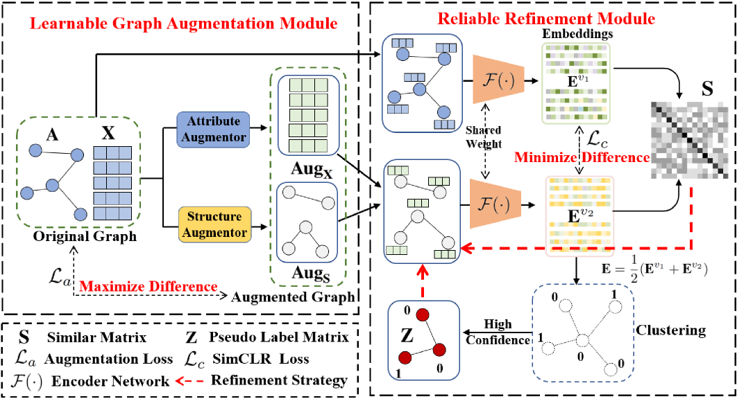
To solve this issue, we propose a fully learnable augmentation strategy for deep contrastive clustering, which generates more suitable augmented views. Specifically, we design the learnable augmenters to learn the structure and attribute information dynamically, thus avoiding the carefully selections of the existing and predefined augmentations. Besides, to improve the reliability of the learned structure, we refine that with the high-confidence clustering pseudo-label matrix and the cross-view sample similarity matrix. Moreover, an adversarial learning mechanism is proposed to learn the consistency of embeddings in latent space, while keeping the diversity of the augmented view. Lastly, during the model training, we present a two-stage training strategy to obtain high-confidence refinement matrices.

By those settings, the augmentation strategies do not rely on tedious manual trial-and-error and repetitive attempts. Moreover, we enhance the connection between the augmentation and the clustering task and integrate the clustering task and the augmentation learning into the unified framework. Firstly, the high-quality augmented graph improves the discriminative capability of embeddings, thus better assisting the clustering task. Meanwhile, the high-confidence clustering results are utilized to refine the augmented graph structure. Concretely, samples within the same clusters are more likely to link, while edges between samples from different clusters are removed.

The key contributions of this paper are listed as follows:

• By designing the structure and attribute augmentor, we propose a learnable data augmentation framework for deep contrastive graph clustering termed AGCLA to dynamically learn the structure and attribute information.

• We refine the augmented graph structure with the cross-view similarity matrix and high-confidence pseudo-label matrix to improve the reliability of the learned affinity matrix. Thus, the clustering task and the augmentation learning are integrated into the unified framework and promote each other.

• Extensive experimental results have demonstrated that AGCLA outperforms the existing state-of-the-art deep graph clustering competitors.

II Related Work

II-A Contrastive Deep Graph Clustering

Clustering is to divide nodes into disjoint clusters [22, 23, 24, 25, 26, 27, 28]. Among those methods, deep graph clustering has attracted great attention in recent years. The existing deep graph clustering methods can be roughly categorized into three classes: generative methods [15, 29, 30, 31, 32, 33, 13, 17], adversarial methods [16, 34, 35], and contrastive methods [36, 37, 14, 38, 39, 18]. More details of deep graph clustering can be found in this survey paper [40]. In recent years, the contrastive learning has achieved great success in vision [41, 42, 43, 44] and graph [45, 46, 47, 48, 49, 50]. In this paper, we focus on the data augmentation of the contrastive deep graph clustering methods. Concretely, a pioneer AGE [36] conducts contrastive learning by a designed adaptive encoder. Besides, MVGRL [37] generates two augmented graph views. Subsequently, DCRN [14] and IDCRN [51] aim to alleviate the collapsed representation by reducing correlation in both sample and feature levels. Meanwhile, the positive and negative sample selection have attracted great attention of researchers. Concretely, GDCL [18] develops a debiased sampling strategy to correct the bias for negative samples. Although promising performance has been achieved, previous methods generate different graph views by adopting uniform data augmentations like graph diffusion, edge perturbation, and feature disturbation. Moreover, these augmentations are manually selected and can not be optimized by the network, thus limiting performance. To solve this problem, we propose a novel contrastive deep graph clustering framework with learnable graph data augmentations.

II-B Data Augmentation in Graph Contrastive Learning

Graph data augmentation [52, 53, 54] is an important component of contrastive learning. The existing data augmentation methods in graph contrastive learning could rough be divided into three categories, i.e., augment-free methods[55], adaptive augmentation methods [56, 57, 19], and learnable data augmentation methods [58, 21, 20, 59]. AFGRL[55] generates the alternative view by discovering nodes that have local and global information without augmentation. While the diversity of the constructed view is limited, leading to poor performance. Furthermore, to make graph augmentation adaptive to different tasks, JOAO [19] learns the sampling distribution of the predefined augmentation to automatically select data augmentation. GCA [56] proposed an adaptive augmentation with incorporating various priors for topological and semantic aspects of the graph. However, the augmentation is still not learnable in the adaptive augmentation methods. Besides, in the field of graph classification, AD-GCL [20] proposed a learnable augmentation for edge-level while neglecting the augmentations on the node level. More recently, AutoGCL[21] proposed a probability-based learnable augmentation. Although promising performance has been achieved, the previous methods still rely on the existing and predefined data augmentations. CONVERT [60] places a strong emphasis on the semantic reliability of augmented views by leveraging a reversible perturb-recover network to generate embeddings for these augmented views. However, it tends to overlook the significance of the underlying graph topology.

In this work, we propose a fully learnable augmentation strategy specifically tailored for graph data. To highlight the uniqueness of our approach, we draw comparisons with existing graph data augmentation methodologies. First and foremost, AGCLA stands out by introducing a completely learnable augmentation approach for graphs. This sets it apart from adaptive augmentation methods such as GCA [56] and JOAO [19], which still rely on predefined augmentations. AGCLA dynamically generates augmented views using a learnable process, considering both structural and attribute aspects of the graph. Moreover, while existing learnable augmentation methods design specific adaptable strategies, they often lack task-specific adaptability. Most of those methods are always graph classification, e.g., AD-GCL [20] and AutoGCL [21]. In contrast, AGCLA addresses this limitation by tailoring the augmentation strategy to graph node clustering in an unsupervised scenario. This ensures that the augmentation is not only learnable but also responsive to downstream task results, enhancing its overall effectiveness.

In summary, AGCLA provides a tailored and learnable augmentation strategy that is agnostic to downstream tasks. By focusing on graph node clustering and incorporating both structural and attribute-level considerations, AGCLA offers a versatile and dynamic approach to graph data augmentation.

III Method

In this section, we propose a novel attribute graph contrastive clustering method with learnable augmentation (AGCLA). The overall framework of AGCLA is shown in Fig.1. The main components of the proposed method include the learnable graph augmentation module and the reliable refinement module. We will detail the proposed AGCLA in the following subsections.

Table I: Notation summary.

Notation	Meaning
$\textbf{X}\in\mathbb{R}^{N\times D}$	Attribute matrix
$\textbf{A}\in\mathbb{R}^{N\times N}$	Original adjacency matrix
$\textbf{D}\in\mathbb{R}^{N\times N}$	Degree matrix
$\textbf{E}^{v_{k}}\in\mathbb{R}^{N\times d}$	Node embeddings in $k$-th view
$\varphi(\cdot)$	Non-parametric metric function
$\textbf{S}\in\mathbb{R}^{N\times N}$	Similarity sample matrix
$\textbf{Z}\in\mathbb{R}^{N\times N}$	High-confidence pseudo label matrix
$\textbf{Aug}_{\textbf{X}}\in\mathbb{R}^{N\times d}$	Augmented attribute matrix
$\textbf{Aug}_{\textbf{S}}\in\mathbb{R}^{N\times N}$	Augmented structure matrix

III-A Notations Definition

For an undirected graph $\textbf{G}=\left\{\textbf{X},\textbf{A}\right\}$. $\textbf{X}\in\mathbb{R}^{N\times D}$ is the attribute matrix, and $\textbf{A}\in\mathbb{R}^{N\times N}$ represents the original adjacency matrix. $\textbf{D}=diag(d_{1},d_{2},\dots,d_{N})\in\mathbb{R}^{N\times N}$ is denoted as the degree matrix, where $d_{i}=\sum_{(v_{i},v_{j})\in\mathcal{E}}a_{ij}$. The normalized graph Laplacian matrix $\textbf{L}=\textbf{D}-\textbf{A}$ is denoted as $\widetilde{\textbf{L}}=\widehat{\textbf{D}}^{-\frac{1}{2}}\widehat{\textbf{L}}\widehat{\textbf{D}}^{-\frac{1}{2}}$. Moreover, we define $\varphi(\cdot)$ as a non-parametric metric function to calculate pair-wise similarity, e.g., cosine similarity function. $\textbf{Aug}_{\textbf{S}}$ and $\textbf{Aug}_{\textbf{X}}$ represent the augmented structure and attribute matrix, respectively. The basic notations are summarized in Table I.

III-B Learnable Graph Augmentation Module

In this subsection, we propose a learnable graph augmentation strategy in both structure and attribute level. To be specific, we design the structure augmentor and attribute augmentor to dynamically learn the structure and attribute, respectively. In the following, we will introduce these augmentors in detail.

MLP-based Structure Augmentor The structure $\textbf{Aug}_{\textbf{S}}$ is learned by the Multi-Layer Perception in MLP structure augmentor as follows:

$$\textbf{A}_{MLP} =\varphi(\textbf{E})=\varphi(MLP(\textbf{A})),$$ (1)

where $\textbf{E}\in\mathbb{R}^{N\times D}$ is the embedding of the original adjacency. Here, we adopt the cosine similarity function as $\varphi(\cdot)$ to calculate the learned structure matrix $\textbf{A}_{MLP}$.

GCN-based Structure Augmentor GCN-based structure generator embeds the attribute matrix X and original adjacency matrix A into embeddings in the latent space. For simplicity, we define the GCN-based structure augmentor as:

$$\textbf{A}_{GCN}=\varphi(\textbf{E})=\sigma(\widetilde{\textbf{D}}^{-\frac{1}{2}}\widetilde{\textbf{A}}\widetilde{\textbf{D}}^{-\frac{1}{2}}\textbf{X}),$$ (2)

similar to Eq.1, E is embedding extracted by the GCN network, e.g., GCN [1], GCN-Cheby [61]. $\sigma(\cdot)$ is a non-linear operation.

Attention-based Structure Augmentor Inspire by GAT [2], we design an attentive network to capture the important structure of the input graph G. To be specific, the normalized attention coefficient matrix $\textbf{A}_{att_{ij}}$ between node $x_{i}$ and $x_{j}$ could be computed as:

$$\textbf{A}_{att_{ij}} =\vec{\textbf{n}}^{T}(\textbf{W}_{x_{i}}||\textbf{W}_{x_{j}}),$$ (3)

$$\textbf{A}_{att_{ij}} =\frac{e^{(\textbf{A}_{att_{ij}})}}{\sum_{k\in\mathcal{N}_{i}}e^{(\textbf{A}_{att_{ik}})}},$$

where $\vec{\textbf{n}}$ and W is the learnable weight vector and weight matrix, respectively. $||$ is the concatenation operation between the weight matrix $\textbf{W}_{x_{i}}$ and $\textbf{W}_{x_{j}}$, and $\mathcal{N}_{i}$ represents the indices the neighbors of node $x_{i}$. By this setting, the model could preserve important topological and semantic graph patterns via the attention mechanism.

To make the augmented view in a fully learnable manner, we design the attribute augmentor to dynamically learn the original attribute.

MLP-based Attribute Augmentor Similar to the MLP-based structure augmentor, we utilize the Multi-Layer Perception (MLP) as the network to learn the original attribute matrix X. The learned attribute matrix $\textbf{Aug}_{\textbf{X}}\in\mathbb{R}^{N\times D}$ can be presented as:

$$\textbf{X}_{MLP} =MLP(\textbf{X}).$$ (4)

where $MLP(\cdot)$ is the MLP network to learn the attribute.

Attention-based Attribute Augmentor To guide the network to take more attention to the important node attributes, we also design an attention-based attribute augmentor. Specifically, we map the node attributes into three different latent spaces:

Q $$=\textbf{W}_{q}\textbf{X}^{T}$$ (5)

K $$=\textbf{W}_{k}\textbf{X}^{T}$$

V $$=\textbf{W}_{v}\textbf{X}^{T}$$

where $\textbf{W}_{q}\in\mathbb{R}^{D\times D},\textbf{W}_{k}\in\mathbb{R}^{D\times D},\textbf{W}_{v}\in\mathbb{R}^{D\times D}$ are the learnable parameter matrices. And $\textbf{Q}\in\mathbb{R}^{D\times N},\textbf{K}\in\mathbb{R}^{D\times N}$ and $\textbf{V}\in\mathbb{R}^{D\times N}$ denotes the query matrix, key matrix and value matrix, respectively.

The attention-based attribute matrix $\textbf{Aug}_{\textbf{X}}$ can be calculated by:

$$\textbf{Aug}_{\textbf{X}}=softmax(\frac{\textbf{K}^{T}\textbf{Q}}{\sqrt{D}})\textbf{V}^{T},$$ (6)

After the structure augmentor and attribute augmentor, we could obtain the augmented view $\textbf{G}^{\prime}=(\textbf{Aug}_{\textbf{S}},\textbf{Aug}_{\textbf{X}})$, which is fully learnable.

Algorithm 1 AGCLA

III-C Reliable Refinement Module

In this subsection, we propose a reliable refinement module to obtain the high-confidence learned graph structure. To be specific, the cross-view sample similarity matrix and the high-confidence matrix are generated to improve the quality of the structure in augmented view. Firstly, we embed the node into the latent space through Eq.7:

$$\textbf{E}=\mathcal{F}(\textbf{G}),$$ (7)

where $\mathcal{F}(\cdot)$ denotes the encoder of our feature extraction framework. Subsequently, we obtain the embeddings of the original view G and the augmented view $\textbf{G}^{\prime}$ with ${\ell^{2}}$-norm as follows:

$$\textbf{E}^{v_{1}} =\mathcal{F}(\textbf{G});$$ (8)

$$\textbf{E}^{v_{2}} =\mathcal{F}(\textbf{G}^{\prime}),$$

In the following, we fuse the two views of the node embeddings as follows:

$$\textbf{E}=\frac{1}{2}(\textbf{E}^{v_{1}}+\textbf{E}^{v_{2}}).$$ (9)

Then we perform K-means [62] on E and obtain the clustering results. After that, we will refine the learned view in two manners, i.e., similarity matrix and pseudo labels matrix refinement.

Similarity Matrix Refinement Through $\mathcal{F}(\cdot)$, we could obtain the embeddings of each view. Subsequently, the similarity matrix S represents the similarity between $i$-th sample in the first view and $j$-th sample in the second view as formulated:

$$\textbf{S}_{ij}=(\textbf{E}_{i}^{v_{1}})^{\text{T}}\textbf{E}_{j}^{v_{2}},i,j\in[1,2,...,N],$$ (10)

where $\textbf{S}_{ij}$ is the cross-view similarity matrix. The proposed similarity matrix S measures the similarity between samples by comprehensively considering attribute and structure information. The connected relationships between different nodes could be reflected by S. Therefore, we utilize S to refine the structure in augmented view with Hadamard product:

$$\textbf{Aug}_{\textbf{S}}=\textbf{Aug}_{\textbf{S}}\odot\textbf{S}.$$ (11)

Pseudo Labels Matrix Refinement To further improve the reliability of the learned structure matrix, we extract reliable clustering information to construct the matrix to further refine the structure in augmented view. Concretely, we utilize the top $\tau$ high-confidence pseudo labels p to construct the matrix as follows:

$$\textbf{Z}_{ij}=\left\{\begin{array}[]{rcl}1&&{\textbf{p}_{i}=\textbf{p}_{j}},\\ 0&&{\textbf{p}_{i}\neq\textbf{p}_{j}}.\end{array}\right.$$ (12)

where $\textbf{Z}_{ij}$ denotes the category relation between $i$-th and $j$-th samples. In detail, when $\textbf{Z}_{ij}=1$, two samples have the same pseudo label. While $\textbf{Z}_{ij}=0$ implies that two samples have different pseudo labels. The pseudo-label matrix is constructed by the high-confidence category information. Therefore, the adjacency relation in the graph could be well reflected, leading to optimizing the structure of the learned structure in the augmented view. The pseudo labels matrix refines the learned structure with Hadamard product as:

$$\textbf{Aug}_{\textbf{S}}=\textbf{Aug}_{\textbf{S}}\odot\textbf{Z}.$$ (13)

In summary, in this subsection, we propose two strategies to refine the structure of the augmented view. Firstly, S is calculated by the cross-view similarity. The value of S represents the probability of connection relationships of the nodes. The structure of $\textbf{Aug}_{\textbf{S}}$ is optimized by S in the training process. Besides, we utilize the high-confidence clustering pseudo labels to construct the reliable node connection, which is constructed when the node belongs to the same category. By those settings, the learned structure is regularized by the similarity matrix and the high-confidence matrix, thus improving the reliability of the structure in the augmented view. Moreover, the connection between augmentation and the clustering task is enhanced.

III-D Loss Function

The proposed AGCLA framework follows the common contrastive learning paradigm, where the model maximizes the agreement of the cross-view [56, 63, 64, 65]. In detail, AGCLA jointly optimizes two loss functions, including the learnable augmentation loss $\mathcal{L}_{a}$ and the contrastive loss $\mathcal{L}_{c}$.

To be specific, $\mathcal{L}_{a}$ is the Mean Squared Error (MSE) loss between the original graph $\textbf{G}=\{\textbf{X},\textbf{A}\}$ and the learnable graph $\textbf{G}^{\prime}=\{\textbf{Aug}_{\textbf{X}},\textbf{Aug}_{\textbf{S}}\}$, which can be formulated as:

$$\mathcal{L}_{a}=-(\left\|\textbf{A}-\textbf{Aug}_{\textbf{S}}\right\|^{2}_{2}+\left\|\textbf{X}-\textbf{Aug}_{\textbf{X}}\right\|^{2}_{2}).$$ (14)

In AGCLA, we utilize the normalized temperature-scaled cross-entropy loss (NT-Xent) to pull close the positive samples, while pushing the negative samples away. The contrastive loss $\mathcal{L}_{c}$ is defined as:

$$l_{i} =-log\frac{\text{exp}(\text{sim}(\textbf{E}^{v_{1}}_{i},\textbf{E}^{v_{2}}_{i})/\text{temp})}{\sum_{k=1,k\neq i}^{N}\text{exp}(\text{sim}(\textbf{E}^{v_{1}}_{i},\textbf{E}^{v_{2}}_{k})/\text{temp})},$$ (15)

$$\mathcal{L}_{c} =\frac{1}{N}\sum_{i=1}^{N}l(i),$$

where temp is a temperature parameter. $\text{sim}(\cdot)$ denotes the function to calculate the similarity, e.g., inner product.

The total loss of AGCLA is calculated as follows:

$$\mathcal{L}=\mathcal{L}_{a}+\alpha\mathcal{L}_{c},$$ (16)

where $\alpha$ is the trade-off between $\mathcal{L}_{a}$ and $\mathcal{L}_{c}$. The first term in Eq.(16) encourages the network to generate the augmented view with distinct semantics to ensure the diversity in input space, while the second term is the contrastive paradigm to learn the consistency of two views in latent space. The discriminative capacity of the network could be improved by minimizing the total loss function. The network is optimized by Eq.(16) during the whole training process. The detailed learning process of AGCLA is shown in Algorithm 1.

The memory cost of $\mathcal{L}$ is acceptable. We utilize $B$ to denote the batch size. The dimension of the embeddings is $D$. The time complexity of $\mathcal{L}$ is $\mathcal{O}(B^{2}D)$. And the space complexity of $\mathcal{L}$ is $\mathcal{O}(B^{2})$ due to matrix multiplication. The detailed experiments are shown in section IV-C. Besides, we design a two-stage training strategy to improve the confidence of the clustering pseudo labels during the overall training procedure. To be specific, the discriminative capacity of the network is improved by the first training stage. Then, in the second stage, we refine the learned structure $\textbf{Aug}_{\textbf{S}}$ in the augmented view with the more reliable similarity matrix and the pseudo labels matrix.

Table II: Dataset information.

Dataset	Type	Sample	Dimension	Edge	Class
CORA	Graph	2708	1433	5429	7
AMAP	Graph	7650	745	119081	8
CITESEER	Graph	3327	3703	4732	6
UAT	Graph	1190	239	13599	4
BAT	Graph	131	81	1038	4
EAT	Graph	399	203	5994	4

Table III: Clustering performance on CORA and BAT datasets (mean ± std). Best results are bold values and the second best values are unerlined.

			CORA				BAT
Methods			ACC (%)	NMI (%)	ARI (%)	F1 (%)	ACC (%)	NMI (%)	ARI (%)	F1 (%)
DEC	[66]	ICML 2016	46.50±0.26	23.54±0.34	15.13±0.42	39.23±0.17	42.09±2.21	14.10±1.99	07.99±1.21	42.63±2.35
DCN	[59]	ICML 2017	49.38±0.91	25.65±0.65	21.63±0.58	43.71±1.05	47.79±3.95	18.03±7.73	13.75±6.05	46.80±3.44
MGAE	[15]	CIKM 2019	43.38±2.11	28.78±2.97	16.43±1.65	33.48±3.05	53.59±2.04	30.59±2.06	24.15±1.70	50.83±3.23
DAEGC	[29]	IJCAI 2019	70.43±0.36	52.89±0.69	49.63±0.43	68.27±0.57	52.67±0.00	21.43±0.35	18.18±0.29	52.23±0.03
ARGA	[16]	TCYB 2019	71.04±0.25	51.06±0.52	47.71±0.33	69.27±0.39	67.86±0.80	49.09±0.54	42.02±1.21	67.02±1.15
SDCN	[13]	WWW 2020	35.60±2.83	14.28±1.91	07.78±3.24	24.37±1.04	53.05±4.63	25.74±5.71	21.04±4.97	46.45±5.90
AdaGAE	[67]	TPAMI 2021	50.06±1.58	32.19±1.34	28.25±0.98	53.53±1.24	43.51±0.48	15.84±0.78	07.80±0.41	43.15±0.77
AGE	[36]	SIGKDD 2020	73.50±1.83	57.58±1.42	50.10±2.14	69.28±1.59	56.68±0.76	36.04±1.54	26.59±1.83	55.07±0.80
MVGRL	[37]	ICML 2020	70.47±3.70	55.57±1.54	48.70±3.94	67.15±1.86	37.56±0.32	29.33±0.70	13.45±0.03	29.64±0.49
DFCN	[17]	AAAI 2021	36.33±0.49	19.36±0.87	04.67±2.10	26.16±0.50	55.73±0.06	48.77±0.51	37.76±0.23	50.90±0.12
GDCL	[18]	IJCAI 2021	70.83±0.47	56.60±0.36	48.05±0.72	52.88±0.97	45.42±0.54	31.70±0.42	19.33±0.57	39.94±0.57
DCRN	[14]	AAAI 2022	61.93±0.47	45.13±1.57	33.15±0.14	49.50±0.42	67.94±1.45	47.23±0.74	39.76±0.87	67.40±0.35
AGC-DRR	[68]	IJCAI 2022	40.62±0.55	18.74±0.73	14.80±1.64	31.23±0.57	47.79±0.02	19.91±0.24	14.59±0.13	42.33±0.51
SLAPS	[69]	NeurIPS 2021	64.21±0.12	41.16±1.24	35.96±0.65	63.72±0.26	41.22±1.25	17.05±0.87	06.86±2.14	37.64±0.57
SUBLIME	[70]	WWW 2022	71.14±0.74	53.88±1.02	50.15±0.14	63.11±0.58	45.04±0.19	22.03±0.48	14.45±0.87	44.00±0.62
GCA	[56]	WWW 2021	53.62±0.73	46.87±0.65	30.32±0.98	45.73±0.47	54.89±0.34	38.88±0.23	26.69±2.85	53.71±0.34
AFGRL	[55]	AAAI 2022	26.25±1.24	12.36±1.54	14.32±1.87	30.20±1.15	50.92±0.44	27.55±0.62	21.89±0.74	46.53±0.57
NACL	[71]	AAAI 2023	51.09±1.25	31.80±0.78	36.66±1.65	51.12±1.12	47.48±0.64	24.36±1.54	24.14±0.98	42.25±0.34
AutoSSL	[58]	ICLR 2022	63.81±0.57	47.62±0.45	38.92±0.77	56.42±0.21	42.43±0.47	17.84±0.98	13.11±0.81	34.84±0.15
AGCLA		Ours	74.91±1.78	58.16±0.83	53.82±2.25	73.33±1.86	75.50±0.87	50.58±0.90	47.45±1.53	75.40±0.88

Table IV: Clustering performance on AMAP and EAT datasets (mean ± std). Best results are bold values and the second best values are unerlined.

			AMAP				EAT
Methods			ACC (%)	NMI (%)	ARI (%)	F1 (%)	ACC (%)	NMI (%)	ARI (%)	F1 (%)
DEC	[66]	ICML 2016	47.22±0.08	37.35±0.05	18.59±0.04	46.71±0.12	36.47±1.60	04.96±1.74	03.60±1.87	34.84±1.28
DCN	[59]	ICML 2017	48.25±0.08	38.76±0.30	20.80±0.47	47.87±0.20	38.85±2.32	06.92±2.80	05.11±2.65	38.75±2.25
MGAE	[15]	CIKM 2019	71.57±2.48	62.13±2.79	48.82±4.57	68.08±1.76	44.61±2.10	15.60±2.30	13.40±1.26	43.08±3.26
DAEGC	[29]	IJCAI 2019	75.96±0.23	65.25±0.45	58.12±0.24	69.87±0.54	36.89±0.15	05.57±0.06	05.03±0.08	34.72±0.16
ARGA	[16]	TCYB 2019	69.28±2.30	58.36±2.76	44.18±4.41	64.30±1.95	52.13±0.00	22.48±1.21	17.29±0.50	52.75±0.07
SDCN	[13]	WWW 2020	53.44±0.81	44.85±0.83	31.21±1.23	50.66±1.49	39.07±1.51	08.83±2.54	06.31±1.95	33.42±3.10
AdaGAE	[67]	TPAMI 2021	67.70±0.54	55.96±0.87	46.20±0.45	62.95±0.74	32.83±1.24	04.36±1.87	02.47±0.54	32.39±0.47
AGE	[36]	SIGKDD 2020	75.98±0.68	65.38±0.61	55.89±1.34	71.74±0.93	47.26±0.32	23.74±0.90	16.57±0.46	45.54±0.40
MVGRL	[37]	ICML 2020	41.07±3.12	30.28±3.94	18.77±2.34	32.88±5.50	32.88±0.71	11.72±1.08	04.68±1.30	25.35±0.75
DFCN	[17]	AAAI 2021	76.82±0.23	66.23±1.21	58.28±0.74	71.25±0.31	49.37±0.19	32.90±0.41	23.25±0.18	42.95±0.04
GDCL	[18]	IJCAI 2021	43.75±0.78	37.32±0.28	21.57±0.51	38.37±0.29	33.46±0.18	13.22±0.33	04.31±0.29	25.02±0.21
DCRN	[14]	AAAI 2022	OOM	OOM	OOM	OOM	50.88±0.55	22.01±1.23	18.13±0.85	47.06±0.66
AGC-DRR	[68]	IJCAI 2022	76.81±1.45	66.54±1.24	60.15±1.56	71.03±0.64	37.37±0.11	07.00±0.85	04.88±0.91	35.20±0.17
SLAPS	[69]	NeurIPS 2021	60.09±1.14	51.15±0.87	42.87±0.75	47.73±0.98	48.62±1.65	28.33±2.56	24.59±0.58	40.42±1.44
SUBLIME	[70]	WWW 2022	27.22±1.56	06.37±1.89	05.36±2.14	15.97±1.53	38.80±0.35	14.96±0.75	10.29±0.88	32.31±0.97
GCA	[56]	WWW 2021	56.81±1.44	48.38±2.38	26.85±0.44	53.59±0.57	48.51±1.55	28.36±1.23	19.61±1.25	48.22±0.33
AFGRL	[55]	AAAI 2022	75.51±0.77	64.05±0.15	54.45±0.48	69.99±0.34	37.42±1.24	11.44±1.41	06.57±1.73	30.53±1.47
NACL	[71]	AAAI 2023	67.18±0.75	63.63±1.07	46.30±1.59	72.04±1.08	36.06±1.24	21.46±1.80	21.48±0.64	31.25±0.96
AutoSSL	[58]	ICLR 2022	54.55±0.97	48.56±0.71	26.87±0.34	54.47±0.83	31.33±0.52	17.63±0.85	12.13±0.67	21.82±0.98
AGCLA		Ours	77.24±0.87	67.12±0.92	58.14±0.82	73.02±2.34	57.22±0.73	33.47±0.34	26.21±0.81	57.53±0.67

Table V: Clustering performance on UAT and CITESEER datasets (mean ± std). Best results are bold values and the second best values are unerlined.

			UAT				CITESEER
Method			ACC (%)	NMI (%)	ARI (%)	F1 (%)	ACC (%)	NMI (%)	ARI (%)	F1 (%)
DEC	[66]	ICML 2016	45.61±1.84	16.63±2.39	13.14±1.97	44.22±1.51	55.89±0.20	28.34±0.30	28.12±0.36	52.62±0.17
DCN	[59]	ICML 2017	46.82±1.14	17.18±1.60	13.59±2.02	45.66±1.49	57.08±0.13	27.64±0.08	29.31±0.14	53.80±0.11
MGAE	[15]	CIKM 2019	48.97±1.52	20.69±0.98	18.33±1.79	47.95±1.52	61.35±0.80	34.63±0.65	33.55±1.18	57.36±0.82
DAEGC	[29]	IJCAI 2019	52.29±0.49	21.33±0.44	20.50±0.51	50.33±0.64	64.54±1.39	36.41±0.86	37.78±1.24	62.20±1.32
ARGA	[16]	TCYB 2019	49.31±0.15	23.44±0.31	16.57±0.31	50.26±0.16	61.07±0.49	34.40±0.71	34.32±0.70	58.23±0.31
SDCN	[13]	WWW 2020	52.25±1.91	21.61±1.26	21.63±1.49	45.59±3.54	65.96±0.31	38.71±0.32	40.17±0.43	63.62±0.24
AdaGAE	[67]	TPAMI 2021	52.10±0.87	26.02±0.71	20.47±0.13	43.44±0.85	54.01±1.11	27.79±0.47	24.19±0.85	51.11±0.64
AGE	[36]	SIGKDD 2020	52.37±0.42	23.64±0.66	20.39±0.70	50.15±0.73	69.73±0.24	44.93±0.53	45.31±0.41	64.45±0.27
MVGRL	[37]	ICML 2020	44.16±1.38	21.53±0.94	17.12±1.46	39.44±2.19	62.83±1.59	40.69±0.93	34.18±1.73	59.54±2.17
DFCN	[17]	AAAI 2021	33.61±0.09	26.49±0.41	11.87±0.23	25.79±0.29	69.50±0.20	43.90±0.20	45.50±0.30	64.30±0.20
GDCL	[18]	IJCAI 2021	48.70±0.06	25.10±0.01	21.76±0.01	45.69±0.08	66.39±0.65	39.52±0.38	41.07±0.96	61.12±0.70
DCRN	[14]	AAAI 2022	49.92±1.25	24.09±0.53	17.17±0.69	44.81±0.87	69.86±0.18	44.86±0.35	45.64±0.30	64.83±0.21
AGC-DRR	[68]	IJCAI 2022	42.64±0.31	11.15±0.24	09.50±0.25	35.18±0.32	68.32±1.83	43.28±1.41	45.34±2.33	64.82±1.60
SLAPS	[69]	NIPS 2021	49.77±1.24	12.86±0.65	17.36±0.98	10.56±1.34	64.14±0.65	39.08±0.25	39.27±0.78	61.00±0.15
SUBLIME	[70]	WWW 2022	48.74±0.54	21.85±0.62	19.51±0.45	46.19±0.87	68.25±1.21	43.15±0.14	44.21±0.54	63.12±0.42
GCA	[56]	WWW 2021	39.39±1.46	24.05±0.25	14.37±0.19	35.72±0.28	60.45±1.03	36.15±0.78	35.20±0.96	56.42±0.94
AFGRL	[55]	AAAI 2022	41.50±0.25	17.33±0.54	13.62±0.57	36.52±0.89	31.45±0.54	15.17±0.47	14.32±0.78	30.20±0.71
NACL	[71]	AAAI 2023	45.38±1.15	24.49±0.57	21.34±0.78	30.56±0.25	59.23±2.32	36.68±0.89	33.37±0.53	52.67±0.64
AutoSSL	[58]	ICLR 2022	42.52±0.64	17.86±0.22	13.13±0.71	34.94±0.87	66.76±0.67	40.67±0.84	38.73±0.55	58.22±0.68
AGCLA		Ours	55.31±2.42	24.40±1.69	22.14±1.67	52.77±2.61	70.12±0.36	43.56±0.35	44.85±0.69	65.01±0.39

Table VI: Ablation studies over the learnable graph augmentation module of AGCLA on six datasets. “(w/o) $\textbf{Aug}_{\textbf{X}}$”, “(w/o) $\textbf{Aug}_{\textbf{S}}$” and “(w/o) $\textbf{Aug}_{\textbf{X}}$ & $\textbf{Aug}_{\textbf{S}}$” represent the reduced models by removing the structure augmentor, the attribute augmentor, and both, respectively. Additionally, our algorithm is compared with four classic data augmentations.

Dataset	Metric	(w/o) Aug_X	(w/o) Aug_S	(w/o) Aug_X & Aug_S	Mask Feature	Drop Edges	Add Edges	Diffusion	Ours
	ACC	65.60±4.95	71.92±1.32	62.16±2.57	70.60±0.91	60.29±2.42	68.02±1.93	72.68±1.00	74.91±1.78
	NMI	48.81±3.95	53.82±1.99	40.84±1.45	53.99±1.48	48.40±1.91	50.78±1.93	55.80±1.22	58.16±0.83
	ARI	42.42±5.09	49.20±1.56	34.84±2.82	47.80±1.09	39.78±2.21	43.56±1.83	50.45±1.24	53.82±2.25
CORA	F1	60.86±8.35	69.82±0.88	60.46±3.10	69.39±0.85	55.40±4.64	66.93±1.96	69.11±0.78	73.33±1.86
	ACC	73.18±4.67	73.14±1.10	68.32±0.98	72.73±0.41	64.22±4.15	74.51±0.16	72.99±0.53	77.24±0.87
	NMI	61.27±5.13	60.99±0.75	53.76±1.12	61.99±0.59	53.07±3.57	62.94±0.28	61.57±0.92	67.12±0.92
	ARI	51.89±6.11	52.27±1.72	44.50±1.28	49.98±0.83	46.07±3.58	53.45±0.32	50.64±0.67	58.14±0.82
AMAP	F1	69.19±4.57	68.73±1.39	63.58±0.93	68.36±0.85	56.14±5.21	69.16±0.14	68.16±0.57	73.02±2.34
	ACC	69.01±2.58	70.84±2.64	64.43±2.35	58.85±3.14	53.28±2.60	66.03±3.19	56.95±3.63	75.50±0.87
	NMI	46.52±1.00	47.96±2.04	40.98±2.30	38.04±2.80	28.44±2.01	41.05±3.20	37.79±4.76	50.58±0.90
	ARI	42.16±1.43	42.97±2.08	35.19±2.96	25.67±4.52	20.86±2.67	36.03±4.28	29.43±3.67	47.45±1.53
BAT	F1	67.05±4.28	70.03±3.71	63.08±3.08	57.94±3.94	52.27±3.00	65.09±3.15	49.84±4.73	75.40±0.88
	ACC	56.42±1.57	55.31±0.88	38.80±1.67	50.13±2.11	47.19±1.81	40.03±5.50	45.56±1.86	57.22±0.73
	NMI	33.11±1.34	32.65±1.02	12.06±2.35	25.74±2.54	28.25±4.64	09.01±7.18	21.12±3.12	33.47±0.34
	ARI	26.66±0.95	25.70±0.86	07.72±2.55	18.46±2.48	22.37±4.43	07.72±6.23	16.28±4.00	26.21±0.81
EAT	F1	56.36±1.99	54.51±2.79	31.53±2.62	48.40±4.36	44.39±2.37	38.57±5.36	36.22±2.63	57.53±0.67
	ACC	48.54±0.54	57.86±0.67	39.25±0.85	63.62±1.10	66.00±1.47	64.16±1.06	65.74±0.56	70.12±0.36
	NMI	20.23±0.23	30.73±0.84	27.67±0.41	39.13±1.17	39.46±1.44	39.35±1.13	40.98±0.57	43.56±0.35
	ARI	13.34±0.66	27.13±0.45	12.57±0.72	37.09±1.73	38.66±2.24	37.78±1.43	39.66±0.91	44.85±0.69
CITESEER	F1	43.50±0.42	54.73±0.58	30.40±0.28	60.36±0.85	58.50±1.24	60.39±1.01	62.00±0.81	65.01±0.39
	ACC	47.61±1.52	49.83±1.17	45.65±0.66	47.09±2.19	53.09±0.71	50.47±1.31	52.39±2.00	55.31±2.42
	NMI	21.66±1.42	25.46±0.62	18.50±1.25	16.79±2.90	22.61±0.67	23.20±1.43	23.30±1.26	24.40±1.69
	ARI	17.71±1.90	21.62±1.06	14.46±1.72	11.82±3.19	21.00±1.58	14.64±2.76	22.17±2.43	22.14±1.67
UAT	F1	43.01±2.30	47.69±1.64	45.58±0.80	45.04±2.37	51.32±0.86	50.26±2.45	48.81±2.62	52.77±2.61

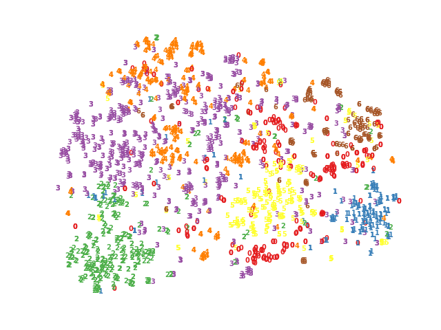
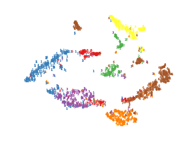
DAEGC

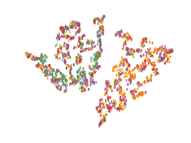
SDCN

AFGRL

GCA

AutoSSL

SUBLIME

Ours

Figure 2: 2D $t$-SNE visualization of seven methods on two benchmark datasets. The first row and second row corresponds to CORA and AMAP dataset, respectively.

IV Experiment

In this section, we implement experiments to verify the superiority of our proposed AGCLA by answering the following questions:

• RQ1: How effective is AGCLA for attribute node clustering?

• RQ2: How about the efficiency about AGCLA?

• RQ3: How does the proposed module influence the performance of AGCLA?

• RQ4: How do the hyper-parameters impact the performance of AGCLA?

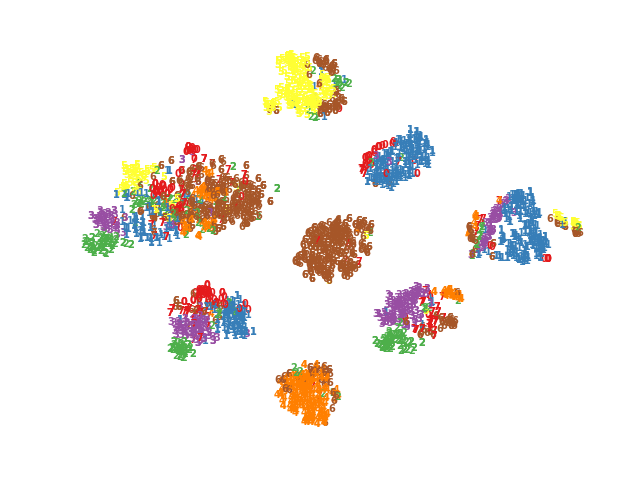
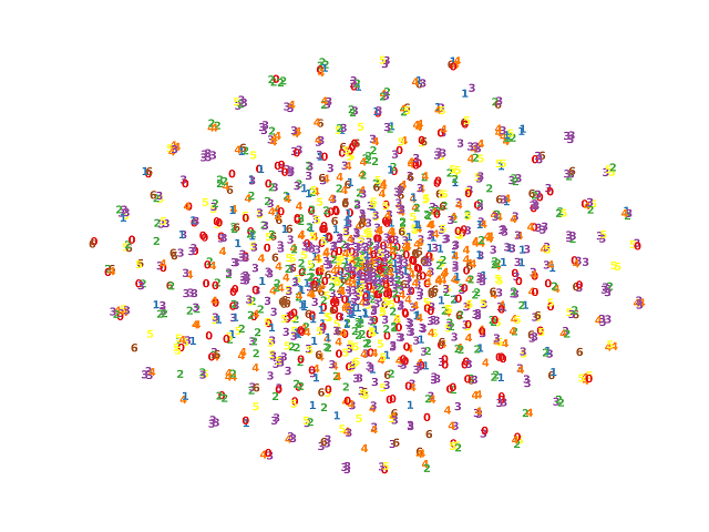
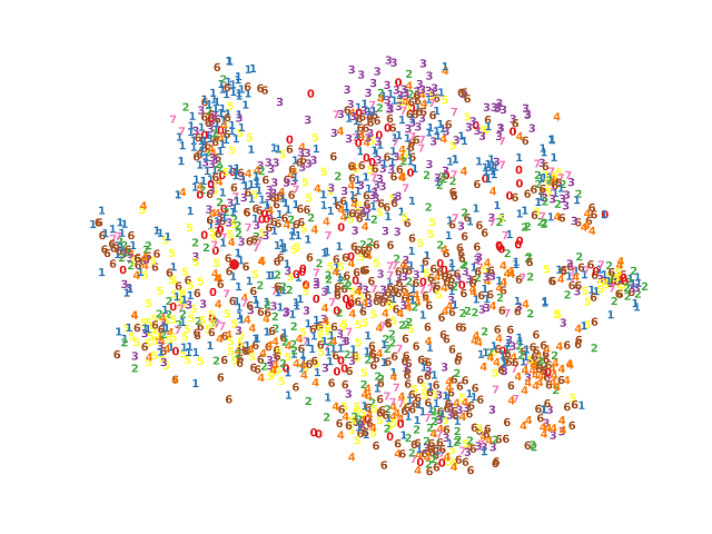
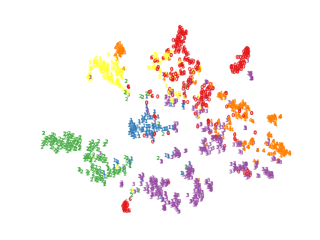
• RQ5: What is the clustering structure revealed by AGCLA?

IV-A Experimental Setup

Benchmark Datasets The experiments are implemented on six widely-used benchmark datasets, including CORA [36], BAT [72], EAT [72], AMAP [14], CITESEER , and UAT [72]. The summarized information is shown in Table II.

Training Details The experiments are conducted on the PyTorch deep learning platform with the Intel Core i7-7820x CPU, one NVIDIA GeForce RTX 2080Ti GPU, 64GB RAM. The max training epoch number is set to 400. For fairness, we conduct ten runs for all methods. For the baselines, we adopt their source with original settings and reproduce the results.

Evaluation Metrics The clustering performance is evaluated by four metrics, including Accuracy (ACC), Normalized Mutual Information (NMI), Average Rand Index (ARI), and macro F1-score (F1) [73, 74, 75].

Parameter Setting In our model, the learning rate is set to 1e-3 for UAT, 1e-4 for CORA/CITESEER, 1e-5 for AMAP/BAT, and 1e-7 for EAT, respectively. The threshold $\tau$ is set to 0.95 for all datasets. The epoch to begin the second training stage $num$ is set to 200. The trade-off $\alpha$ is set to 0.5.

CORA

AMAP

EAT

UAT

BAT

BAT

Figure 3: Ablation studies over the effectiveness of the proposed similarity matrix and pseudo labels matrix refinement strategy on six benchmark datasets.“NP+NS”, “NP”, “NS”, and “P+S” denotes the baseline, baseline with similarity matrix optimization, baseline with pseudo-label matrix optimization, and ours, respectively.

CORA

BAT

AMAP

EAT

UAT

CITESEER

Figure 4: Sensitivity analysis of the hyper-parameter $\tau$.

CORA

BAT

AMAP

EAT

UAT

CITESEER

Figure 5: Sensitivity analysis of the hyper-parameter $\alpha$.

IV-B Performance Comparison (RQ1)

In this subsection, to verify the superiority of AGCLA, we compare the clustering performance of our proposed algorithm with 19 baselines on six datasets with four metrics. We divide these methods into four categories, i.e., classical deep clustering methods (DEC [66], DCN [59], MGAE [76], DAEGC [29], ARGA [16], SDCN [13], AdaGAE[67]), contrastive deep graph clustering methods (AGE [36], MVGRL [37], DFCN[17], GDCL[18], DCRN [14], AGC-DRR [68]), graph structure learning methods (SLAPS [69], SUBLIME [70]), and graph augmentation methods (GCA [56], AFGRL [55], NACL [71], AutoSSL [58]).

Here, we adopt the attention structure augmentor and the MLP attribute augmentor to generate the augmented view in a learnable way. The results are shown in Table.III, Table.V and Table.IV, we observe and analyze as follows:

• AGCLA obtains better performance compared with classical deep clustering methods. The reason is that they rarely consider the topological information in the graph.

• Contrastive deep graph clustering methods achieve sub-optimal performance compared with ours. We conjecture that the discriminative capacity of our AGCLA is improved with learnable augmentation and optimization strategies.

• The classical graph augmentation methods achieve unsatisfied clustering performance. This is because they merely consider the learnable of the structure, while neglecting the attribute. Moreover, most of those methods can not optimize with the downstream tasks.

• It could be observed that the graph structure learning methods are not comparable with ours. We analyze the reason is that those methods refine the structure with the unreliable strategy at the beginning of the training. In summary, our method outperforms most of other algorithms on six datasets with four metrics. Taking the result on CORA dataset for example, AGCLA exceeds the runner-up by 1.41%, 0.58%, 3.72%, 4.05% with respect to ACC, NMI, ARI, and F1.

Moreover, we implement experiments on other augmentors. The results are shown in Table. VIII, we conclude that our proposed augmentors could achieve better performance on most metrics compared with other graph clustering algorithms.

Figure 6: GPU memory costs on six datasets with five methods.

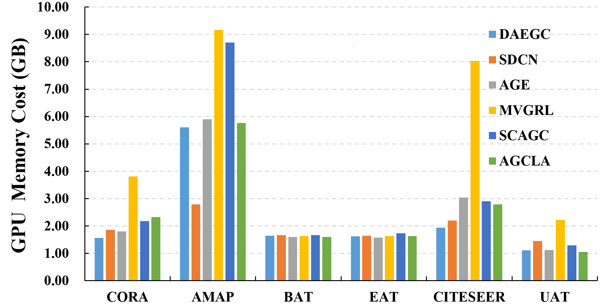
IV-C Time Cost and Memory Cost (RQ2)

In this subsection, we implement time and memory cost experiments to demonstrate the effectiveness of the proposed AGCLA.

Specifically, we test the training time of AGCLA with five baselines on six datasets. For fairness, we train all algorithms with 400 epochs. From the results in Table VII, we observe that the training time of AGCLA is comparable with other eight algorithms. The reason we analyze is as follows: instead of using GCN as the encoder network, we adopt the graph filter to smooth the feature. This operation effectively reduces time consumption.

Moreover, we conduct experiments to test GPU memory costs of our proposed AGCLA with five methods (i.e., DAEGC [29], SDCN [13], AGE [36], MVGRL [37], SCAGC [38] ) on six datasets. From the results in Fig. 6, we observe that the memory costs of our AGCLA are also comparable with other algorithms.

IV-D Ablation Studies (RQ3)

In this section, we first conduct ablation studies to verify the effectiveness of the proposed modules, and then we analyze the robustness of AGCLA to the hyper-parameters. Last, we conduct experiments to verify the effectiveness of our proposed loss function.

IV-D1 Effectiveness of the Structure and Attribute Augmentor

To verify the effect of the proposed structure and attribute augmentor, we conduct extensive experiments as shown in Table VI. Here, we adopt “(w/o) $\textbf{Aug}_{\textbf{X}}$”, “(w/o) $\textbf{Aug}_{\textbf{S}}$” and “(w/o) $\textbf{Aug}_{\textbf{X}}$ & $\textbf{Aug}_{\textbf{S}}$” to represent the reduced models by removing the structure augmentor, the attribute augmentor, and both, respectively. From the observations, it is apparent that the performance will decrease without any of our proposed augmentors, revealing that both augmentors make essential contributions to boosting the performance. Taking the result on the CORA dataset for example, the model performance is improved substantially by utilizing the attribute augmentor.

IV-D2 Effectiveness of the Similarity and Pseudo-label Matrix Optimization

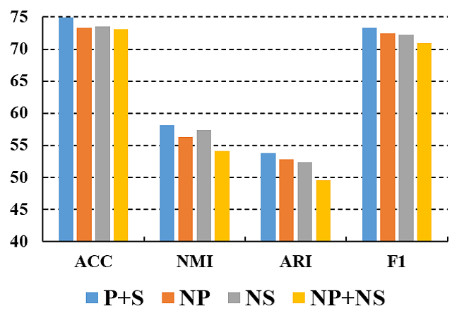
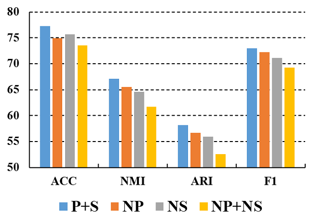
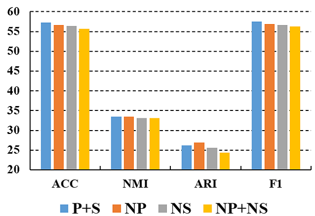
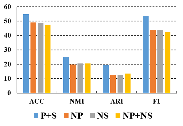
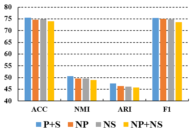
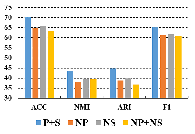
In this subsection, we implement experiments to verify the effectiveness of our optimization strategies, i.e., similarity matrix optimization and pseudo-label matrix optimization. Here, we adopt the model without any optimization strategy as the baseline. For simplicity, we denote “NP+NS”, “NP”, “NS”, and “P+S” as the baseline, baseline with similarity matrix optimization, baseline with pseudo-label matrix optimization, and ours, respectively. From the results in Fig. 3, we observe that the performance of the AGCLA will decrease when any one of the aforementioned components is dropped. Overall, extensive experiments could demonstrate the effectiveness of our optimization strategies.

IV-D3 Effectiveness of our learnable augmentation

To avoid the existing and predefined augmentations on graphs, we design a novel learnable augmentation method for graph clustering. In this part, we compare our view construction method with other classical graph data augmentations, including mask feature [18], drop edges [38], add edges [38], and graph diffusion [51]. Concretely, in Table VI, we adopt the data augmentation as randomly dropping 20% edges (“Drop Edges”), or randomly adding 20% edges (“Add Edges”), or graph diffusion (“Diffusion”) with 0.20 teleportation rate, or randomly masking 20% features (“Mask Feature”). From the results, we observe that the performance of commonly used graph augmentations is not comparable with ours. In summary, extensive experiments have demonstrated the effectiveness of the proposed learnable augmentation.

IV-E Hyper-parameter Analysis (RQ4)

Table VII: Training Time Comparison on six datasets with nine methods. The algorithms are measured by seconds. The Avg. represents the average time cost on five datasets.

Method	CORA	AMAP	EAT	CITESEER	UAT	Avg.
DEC	91.13	264.20	26.99	223.95	42.30	129.71
DCN	47.31	94.48	9.56	74.69	29.57	51.12
DAEGC	12.97	39.62	5.14	14.70	6.44	15.77
MGAE	7.38	18.64	4.64	6.69	4.75	8.42
AGE	46.65	377.49	3.86	70.63	8.95	101.52
MVGRL	14.72	131.38	3.32	18.31	4.27	64.4
SCAGC	54.08	150.54	47.79	50.00	64.70	73.42
Ours	10.06	83.26	2.21	17.24	4.15	23.38

Table VIII: Clustering performance on other augmentors.

Method	Metric	CORA	AMAP	BAT	EAT	UAT
X_ATT&A_GCN	ACC	74.48	77.76	74.89	57.89	56.02
	NMI	54.95	65.97	50.37	34.07	26.09
	ARI	51.09	58.70	46.42	27.32	22.87
	F1	73.79	69.89	74.97	58.05	55.49
X_ATT&A_MLP	ACC	73.91	77.58	72.06	57.22	55.18
	NMI	57.92	66.74	47.24	33.77	23.73
	ARI	49.58	58.47	42.48	27.38	21.92
	F1	70.70	72.21	71.86	56.40	52.28
X_ATT&A_ATT	ACC	74.37	77.22	74.96	57.52	55.33
	NMI	55.30	66.71	50.04	33.67	25.17
	ARI	50.57	57.53	46.40	27.05	21.40
	F1	73.95	72.65	75.04	57.62	55.36
X_MLP&A_GCN	ACC	74.70	77.29	73.44	56.97	52.04
	NMI	56.54	66.14	51.55	33.07	22.08
	ARI	50.80	57.04	47.26	26.05	17.20
	F1	74.47	70.96	71.93	57.25	48.01
X_MLP&A_MLP	ACC	73.97	77.54	75.19	56.89	55.60
	NMI	55.07	66.59	50.20	33.48	24.99
	ARI	49.80	58.14	46.78	26.37	24.38
	F1	73.55	72.47	75.25	57.09	53.97
X_MLP&A_ATT	ACC	74.91	77.24	75.50	57.22	55.31
	NMI	58.16	67.12	50.58	33.47	24.40
	ARI	53.82	58.14	47.45	26.21	22.14
	F1	73.33	73.02	75.40	57.53	52.77

IV-E1 Sensitivity Analysis of hyper-parameter $\alpha$

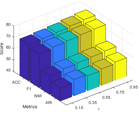
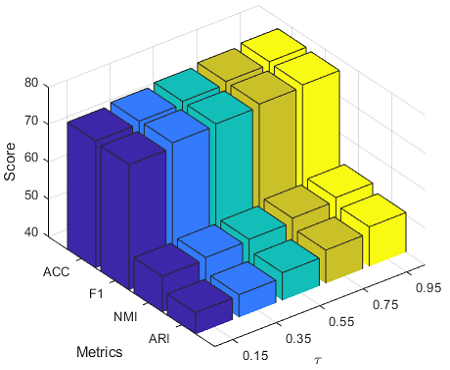
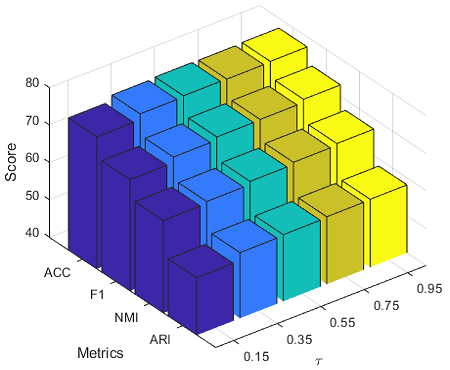
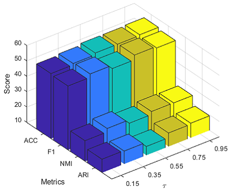
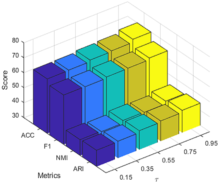
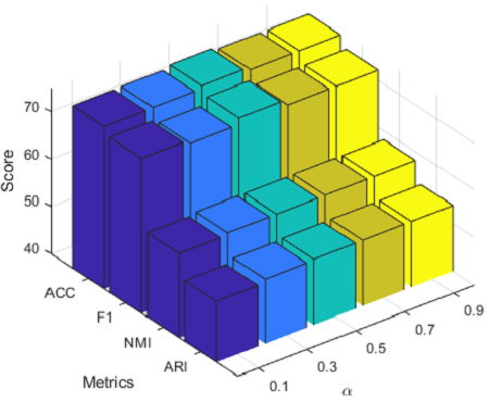
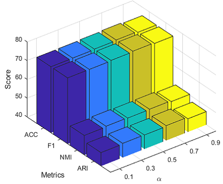
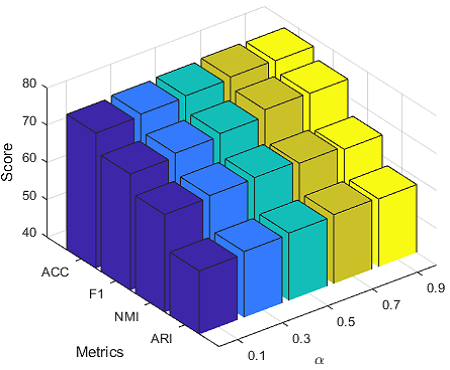
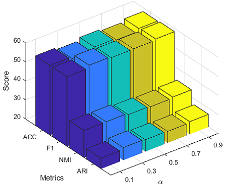
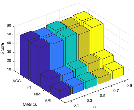
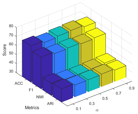
We verify the sensitivity of $\alpha$. The experimental results are shown in Fig.5. The performance will not fluctuate greatly when $\alpha\in[0.1,0.9]$. From these results, we observe that our AGCLA is insensitive to $\alpha$.

IV-E2 Sensitivity Analysis of hyper-parameter $\tau$

As shown in Fig.4, we conduct experiments on six datasets to investigate the influence of the hyper-parameter threshold $\tau$. From the results, we observe that the model obtains promising performance with the $\tau$ increasing. The reason is that the pseudo labels are more reliable with high threshold.

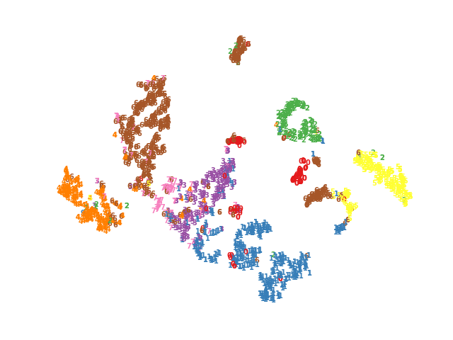
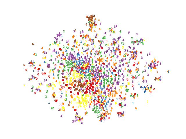
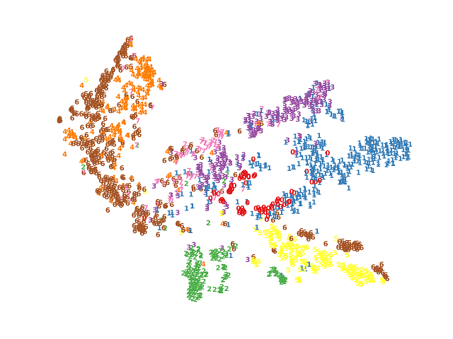
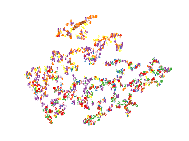
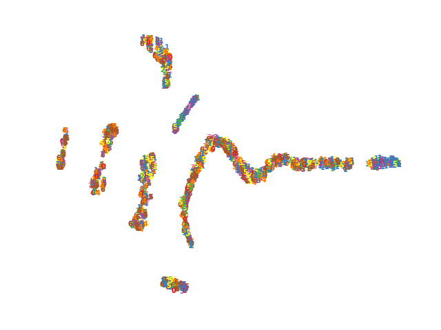
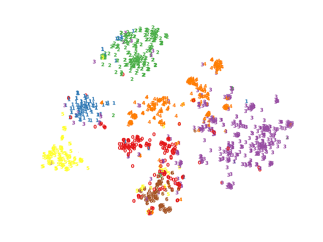
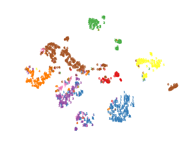
IV-F Visualization Analysis (RQ5)

In this subsection, we visualize the distribution of the learned embeddings to show the superiority of AGCLA on CORA and AMAP datasets via $t$-SNE algorithm [77]. Six baselines and AGCLA are shown in Fig. 2. We can conclude that AGCLA better reveals the intrinsic clustering structure.

V Conclusion

In this work, we propose a learnable augmentation method for graph contrastive clustering termed AGCLA. To be specific, we design a fully learnable augmentation with the structure augmentor and the attribute augmentor to dynamically learn the structure and attribute information, respectively. Besides, an adversarial mechanism is designed to keep cross-view consistency in the latent space while ensuring the diversity of the augmented views. Meanwhile, we propose a two-stage training strategy to obtain more reliable clustering information during the model training. Benefiting from the clustering information, we refine the learned structure with the high-confidence pseudo-label matrix. Moreover, we refine the augmented view with the cross-view sample similarity matrix to further improve the discriminative capability of the learned structure. Extensive experiments on six datasets demonstrate the effectiveness of our proposed method. In the future, it is worth trying the augmentors designed in AGCLA for other graph downstream tasks, e.g., node classification and link prediction.

References

- [1] T. N. Kipf and M. Welling, “Semi-supervised classification with graph convolutional networks,” in International Conference on Learning Representations, 2017.
- [2] P. Veličković, G. Cucurull, A. Casanova, A. Romero, P. Lio, and Y. Bengio, “Graph attention networks,” arXiv preprint arXiv:1710.10903, 2017.
- [3] J. Xia, L. Wu, G. Wang, J. Chen, and S. Z. Li, “Progcl: Rethinking hard negative mining in graph contrastive learning,” in International Conference on Machine Learning. PMLR, 2022, pp. 24 332–24 346.
- [4] X. Yang, Y. Liu, S. Zhou, X. Liu, and E. Zhu, “Mixed graph contrastive network for semi-supervised node classification,” arXiv preprint arXiv:2206.02796, 2022.
- [5] J. Xia, J. Zheng, C. Tan, G. Wang, and S. Z. Li, “Towards effective and generalizable fine-tuning for pre-trained molecular graph models,” bioRxiv, 2022.
- [6] J. Xia, Y. Zhu, Y. Du, and S. Z. Li, “Pre-training graph neural networks for molecular representations: retrospect and prospect,” in ICML 2022 2nd AI for Science Workshop, 2022.
- [7] Z. Peng, H. Liu, Y. Jia, and J. Hou, “Deep attention-guided graph clustering with dual self-supervision,” IEEE Transactions on Circuits and Systems for Video Technology, 2022.
- [8] Y. Chen, X. Xiao, C. Peng, G. Lu, and Y. Zhou, “Low-rank tensor graph learning for multi-view subspace clustering,” IEEE Transactions on Circuits and Systems for Video Technology, vol. 32, no. 1, pp. 92–104, 2021.
- [9] G. Jiang, J. Peng, H. Wang, Z. Mi, and X. Fu, “Tensorial multi-view clustering via low-rank constrained high-order graph learning,” IEEE Transactions on Circuits and Systems for Video Technology, vol. 32, no. 8, pp. 5307–5318, 2022.
- [10] Z. Li, Y. Li, L. Tang, T. Zhang, and J. Su, “Two-person graph convolutional network for skeleton-based human interaction recognition,” IEEE Transactions on Circuits and Systems for Video Technology, 2022.
- [11] L. Wang, X. Liu, X. Ma, J. Wu, J. Cheng, and M. Zhou, “A progressive quadric graph convolutional network for 3d human mesh recovery,” IEEE Transactions on Circuits and Systems for Video Technology, vol. 33, no. 1, pp. 104–117, 2022.
- [12] X. Xiong, W. Min, Q. Wang, and C. Zha, “Human skeleton feature optimizer and adaptive structure enhancement graph convolution network for action recognition,” IEEE Transactions on Circuits and Systems for Video Technology, vol. 33, no. 1, pp. 342–353, 2022.
- [13] D. Bo, X. Wang, C. Shi, M. Zhu, E. Lu, and P. Cui, “Structural deep clustering network,” in Proceedings of The Web Conference 2020, 2020, pp. 1400–1410.
- [14] Y. Liu, W. Tu, S. Zhou, X. Liu, L. Song, X. Yang, and E. Zhu, “Deep graph clustering via dual correlation reduction,” in AAAI Conference on Artificial Intelligence, 2022.
- [15] C. Wang, S. Pan, G. Long, X. Zhu, and J. Jiang, “Mgae: Marginalized graph autoencoder for graph clustering,” in Proceedings of the 2017 ACM on Conference on Information and Knowledge Management, 2017, pp. 889–898.
- [16] S. Pan, R. Hu, S.-f. Fung, G. Long, J. Jiang, and C. Zhang, “Learning graph embedding with adversarial training methods,” IEEE transactions on cybernetics, vol. 50, no. 6, pp. 2475–2487, 2019.
- [17] W. Tu, S. Zhou, X. Liu, X. Guo, Z. Cai, J. Cheng et al., “Deep fusion clustering network,” arXiv preprint arXiv:2012.09600, 2020.
- [18] H. Zhao, X. Yang, Z. Wang, E. Yang, and C. Deng, “Graph debiased contrastive learning with joint representation clustering,” in Proc. IJCAI, 2021, pp. 3434–3440.
- [19] Y. You, T. Chen, Y. Shen, and Z. Wang, “Graph contrastive learning automated,” in International Conference on Machine Learning. PMLR, 2021, pp. 12 121–12 132.
- [20] S. Suresh, P. Li, C. Hao, and J. Neville, “Adversarial graph augmentation to improve graph contrastive learning,” Advances in Neural Information Processing Systems, vol. 34, pp. 15 920–15 933, 2021.
- [21] Y. Yin, Q. Wang, S. Huang, H. Xiong, and X. Zhang, “Autogcl: Automated graph contrastive learning via learnable view generators,” in Proceedings of the AAAI Conference on Artificial Intelligence, vol. 36, no. 8, 2022, pp. 8892–8900.
- [22] S. Liu, S. Wang, P. Zhang, K. Xu, X. Liu, C. Zhang, and F. Gao, “Efficient one-pass multi-view subspace clustering with consensus anchors,” in Proceedings of the AAAI Conference on Artificial Intelligence, vol. 36, no. 7, 2022, pp. 7576–7584.
- [23] M. Sun, P. Zhang, S. Wang, S. Zhou, W. Tu, X. Liu, E. Zhu, and C. Wang, “Scalable multi-view subspace clustering with unified anchors,” in Proceedings of the 29th ACM International Conference on Multimedia, 2021, pp. 3528–3536.
- [24] Y. Wang, X. Lin, L. Wu, W. Zhang, Q. Zhang, and X. Huang, “Robust subspace clustering for multi-view data by exploiting correlation consensus,” IEEE Transactions on Image Processing, vol. 24, no. 11, pp. 3939–3949, 2015.
- [25] Y. Wang, W. Zhang, L. Wu, X. Lin, M. Fang, and S. Pan, “Iterative views agreement: An iterative low-rank based structured optimization method to multi-view spectral clustering,” arXiv preprint arXiv:1608.05560, 2016.
- [26] Y. Wang and L. Wu, “Beyond low-rank representations: Orthogonal clustering basis reconstruction with optimized graph structure for multi-view spectral clustering,” Neural Networks, vol. 103, pp. 1–8, 2018.
- [27] M. Sun, S. Wang, P. Zhang, X. Liu, X. Guo, S. Zhou, and E. Zhu, “Projective multiple kernel subspace clustering,” IEEE Transactions on Multimedia, vol. 24, pp. 2567–2579, 2021.
- [28] X. Yang, J. Jin, S. Wang, K. Liang, Y. Liu, Y. Wen, S. Liu, S. Zhou, X. Liu, and E. Zhu, “Dealmvc: Dual contrastive calibration for multi-view clustering,” in Proceedings of the 31th ACM International Conference on Multimedia, 2023.
- [29] C. Wang, S. Pan, R. Hu, G. Long, J. Jiang, and C. Zhang, “Attributed graph clustering: A deep attentional embedding approach,” arXiv preprint arXiv:1906.06532, 2019.
- [30] X. Zhang, H. Liu, Q. Li, and X.-M. Wu, “Attributed graph clustering via adaptive graph convolution,” in Proceedings of the 28th International Joint Conference on Artificial Intelligence, 2019, pp. 4327–4333.
- [31] J. Park, M. Lee, H. J. Chang, K. Lee, and J. Y. Choi, “Symmetric graph convolutional autoencoder for unsupervised graph representation learning,” in Proceedings of the IEEE/CVF International Conference on Computer Vision, 2019, pp. 6519–6528.
- [32] J. Cheng, Q. Wang, Z. Tao, D. Xie, and Q. Gao, “Multi-view attribute graph convolution networks for clustering,” in Proceedings of the Twenty-Ninth International Conference on International Joint Conferences on Artificial Intelligence, 2021, pp. 2973–2979.
- [33] Z. Peng, H. Liu, Y. Jia, and J. Hou, “Attention-driven graph clustering network,” in Proceedings of the 29th ACM International Conference on Multimedia, 2021, pp. 935–943.
- [34] S. Pan, R. Hu, G. Long, J. Jiang, L. Yao, and C. Zhang, “Adversarially regularized graph autoencoder for graph embedding,” in Proceedings of the 27th International Joint Conference on Artificial Intelligence, 2018, pp. 2609–2615.
- [35] Z. Tao, H. Liu, J. Li, Z. Wang, and Y. Fu, “Adversarial graph embedding for ensemble clustering,” in International Joint Conferences on Artificial Intelligence Organization, 2019.
- [36] G. Cui, J. Zhou, C. Yang, and Z. Liu, “Adaptive graph encoder for attributed graph embedding,” in Proceedings of the 26th ACM SIGKDD International Conference on Knowledge Discovery & Data Mining, 2020, pp. 976–985.
- [37] K. Hassani and A. H. Khasahmadi, “Contrastive multi-view representation learning on graphs,” in International Conference on Machine Learning. PMLR, 2020, pp. 4116–4126.
- [38] W. Xia, Q. Wang, Q. Gao, M. Yang, and X. Gao, “Self-consistent contrastive attributed graph clustering with pseudo-label prompt,” IEEE Transactions on Multimedia, 2022.
- [39] Y. Liu, X. Yang, S. Zhou, X. Liu, S. Wang, K. Liang, W. Tu, and L. Li, “Simple contrastive graph clustering,” IEEE Transactions on Neural Networks and Learning Systems, 2023.
- [40] Y. Liu, J. Xia, S. Zhou, S. Wang, X. Guo, X. Yang, K. Liang, W. Tu, Z. S. Li, and X. Liu, “A survey of deep graph clustering: Taxonomy, challenge, and application,” arXiv preprint arXiv:2211.12875, 2022.
- [41] T. Chen, S. Kornblith, M. Norouzi, and G. Hinton, “A simple framework for contrastive learning of visual representations,” in International conference on machine learning. PMLR, 2020, pp. 1597–1607.
- [42] J.-B. Grill, F. Strub, F. Altché, C. Tallec, P. H. Richemond, E. Buchatskaya, C. Doersch, B. A. Pires, Z. D. Guo, M. G. Azar et al., “Bootstrap your own latent: A new approach to self-supervised learning,” arXiv preprint arXiv:2006.07733, 2020.
- [43] J. Zbontar, L. Jing, I. Misra, Y. LeCun, and S. Deny, “Barlow twins: Self-supervised learning via redundancy reduction,” arXiv preprint arXiv:2103.03230, 2021.
- [44] X. Chen and K. He, “Exploring simple siamese representation learning,” in Proceedings of the IEEE/CVF Conference on Computer Vision and Pattern Recognition, 2021, pp. 15 750–15 758.
- [45] K. Liang, Y. Liu, S. Zhou, X. Liu, and W. Tu, “Relational symmetry based knowledge graph contrastive learning,” arXiv preprint arXiv:2211.10738, 2022.
- [46] Y. Zhu, Y. Xu, F. Yu, Q. Liu, S. Wu, and L. Wang, “Deep Graph Contrastive Representation Learning,” in ICML Workshop on Graph Representation Learning and Beyond, 2020. [Online]. Available: http://arxiv.org/abs/2006.04131
- [47] J. Xia, L. Wu, J. Chen, B. Hu, and S. Z. Li, “Simgrace: A simple framework for graph contrastive learning without data augmentation,” arXiv preprint arXiv:2202.03104, 2022.
- [48] Y. You, T. Chen, Y. Sui, T. Chen, Z. Wang, and Y. Shen, “Graph contrastive learning with augmentations,” Advances in Neural Information Processing Systems, vol. 33, pp. 5812–5823, 2020.
- [49] Y. Zhu, Y. Xu, Q. Liu, and S. Wu, “An empirical study of graph contrastive learning,” arXiv preprint arXiv:2109.01116, 2021.
- [50] Y. Zhu, Y. Xu, H. Cui, C. Yang, Q. Liu, and S. Wu, “Structure-enhanced heterogeneous graph contrastive learning,” in Proceedings of the 2022 SIAM International Conference on Data Mining (SDM). SIAM, 2022, pp. 82–90.
- [51] Y. Liu, S. Zhou, X. Liu, W. Tu, and X. Yang, “Improved dual correlation reduction network,” arXiv preprint arXiv:2202.12533, 2022.
- [52] L. Yu, S. Pei, L. Ding, J. Zhou, L. Li, C. Zhang, and X. Zhang, “Sail: Self-augmented graph contrastive learning,” in Proceedings of the AAAI Conference on Artificial Intelligence, vol. 36, no. 8, 2022, pp. 8927–8935.
- [53] Y. Wang, W. Wang, Y. Liang, Y. Cai, J. Liu, and B. Hooi, “Nodeaug: Semi-supervised node classification with data augmentation,” in Proceedings of the 26th ACM SIGKDD International Conference on Knowledge Discovery & Data Mining, 2020, pp. 207–217.
- [54] Y. Wang, W. Wang, Y. Liang, Y. Cai, and B. Hooi, “Mixup for node and graph classification,” in Proceedings of the Web Conference 2021, 2021, pp. 3663–3674.
- [55] N. Lee, J. Lee, and C. Park, “Augmentation-free self-supervised learning on graphs,” arXiv preprint arXiv:2112.02472, 2021.
- [56] Y. Zhu, Y. Xu, F. Yu, Q. Liu, S. Wu, and L. Wang, “Graph contrastive learning with adaptive augmentation,” in Proceedings of the Web Conference 2021, 2021, pp. 2069–2080.
- [57] Y. Wang, Y. Cai, Y. Liang, H. Ding, C. Wang, S. Bhatia, and B. Hooi, “Adaptive data augmentation on temporal graphs,” Advances in Neural Information Processing Systems, vol. 34, pp. 1440–1452, 2021.
- [58] W. Jin, X. Liu, X. Zhao, Y. Ma, N. Shah, and J. Tang, “Automated self-supervised learning for graphs,” arXiv preprint arXiv:2106.05470, 2021.
- [59] B. Yang, X. Fu, N. D. Sidiropoulos, and M. Hong, “Towards k-means-friendly spaces: Simultaneous deep learning and clustering,” in international conference on machine learning. PMLR, 2017, pp. 3861–3870.
- [60] X. Yang, C. Tan, Y. Liu, K. Liang, S. Wang, S. Zhou, J. Xia, S. Z. Li, X. Liu, and E. Zhu, “Convert: Contrastive graph clustering with reliable augmentation,” in Proceedings of the 31th ACM International Conference on Multimedia, 2023.
- [61] M. Defferrard, X. Bresson, and P. Vandergheynst, “Convolutional neural networks on graphs with fast localized spectral filtering,” Advances in neural information processing systems, 2016.
- [62] J. A. Hartigan and M. A. Wong, “Algorithm as 136: A k-means clustering algorithm,” Journal of the royal statistical society. series c (applied statistics), vol. 28, no. 1, pp. 100–108, 1979.
- [63] Y. Zhu, Y. Xu, F. Yu, Q. Liu, S. Wu, and L. Wang, “Deep graph contrastive representation learning,” arXiv preprint arXiv:2006.04131, 2020.
- [64] Y. Zhu, Y. Xu, Q. Liu, and S. Wu, “An empirical study of graph contrastive learning,” arXiv preprint arXiv:2109.01116, 2021.
- [65] X. Yang, X. Hu, S. Zhou, X. Liu, and E. Zhu, “Interpolation-based contrastive learning for few-label semi-supervised learning,” IEEE Transactions on Neural Networks and Learning Systems, pp. 1–12, 2022.
- [66] J. Xie, R. Girshick, and A. Farhadi, “Unsupervised deep embedding for clustering analysis,” in International conference on machine learning. PMLR, 2016, pp. 478–487.
- [67] X. Li, H. Zhang, and R. Zhang, “Adaptive graph auto-encoder for general data clustering,” IEEE Transactions on Pattern Analysis and Machine Intelligence, 2021.
- [68] L. Gong, S. Zhou, X. Liu, and W. Tu, “Attributed graph clustering with dual redundancy reduction,” in IJCAI, 2022.
- [69] B. Fatemi, L. El Asri, and S. M. Kazemi, “Slaps: Self-supervision improves structure learning for graph neural networks,” Advances in Neural Information Processing Systems, vol. 34, pp. 22 667–22 681, 2021.
- [70] Y. Liu, Y. Zheng, D. Zhang, H. Chen, H. Peng, and S. Pan, “Towards unsupervised deep graph structure learning,” in Proceedings of the ACM Web Conference 2022, 2022, pp. 1392–1403.
- [71] X. Shen, D. Sun, S. Pan, X. Zhou, and L. T. Yang, “Neighbor contrastive learning on learnable graph augmentation,” arXiv preprint arXiv:2301.01404, 2023.
- [72] N. Mrabah, M. Bouguessa, M. F. Touati, and R. Ksantini, “Rethinking graph auto-encoder models for attributed graph clustering,” arXiv preprint arXiv:2107.08562, 2021.
- [73] S. Zhou, X. Liu, M. Li, E. Zhu, L. Liu, C. Zhang, and J. Yin, “Multiple kernel clustering with neighbor-kernel subspace segmentation,” IEEE transactions on neural networks and learning systems, vol. 31, no. 4, pp. 1351–1362, 2019.
- [74] S. Wang, X. Liu, X. Zhu, P. Zhang, Y. Zhang, F. Gao, and E. Zhu, “Fast parameter-free multi-view subspace clustering with consensus anchor guidance,” IEEE Transactions on Image Processing, vol. 31, pp. 556–568, 2021.
- [75] S. Wang, X. Liu, L. Liu, S. Zhou, and E. Zhu, “Late fusion multiple kernel clustering with proxy graph refinement,” IEEE Transactions on Neural Networks and Learning Systems, 2021.
- [76] T. N. Kipf and M. Welling, “Variational graph auto-encoders,” arXiv preprint arXiv:1611.07308, 2016.
- [77] L. Van der Maaten and G. Hinton, “Visualizing data using t-sne.” Journal of machine learning research, vol. 9, no. 11, 2008.