A mesh-free particle method for continuum modeling of granular flow

Abstract

Based on the continuum model for granular media developed in Dunatunga et al. we propose a mesh-free generalized finite difference method for the simulation of granular flows. The model is given by an elasto-viscoplastic model with a yield criterion using the $\mu(I)$ rheology from Jop et al. The numerical procedure is based on a mesh-free particle method with a least squares approximation of the derivatives in the balance equations combined with the numerical algorithm developed in Dunatunga et al. to compute the plastic stresses. The method is numerically tested and verified for several numerical experiments including granular column collapse and rigid body motion in granular materials. For comparison a nonlinear microscopic model from Lacaze et al. is implemented and results are compared to the those obtained from the continuum model for granular column collapse and rigid body coupling to granular flow.

1 Introduction

Granular materials have been modelled using microscopic and continuum approaches in many works. The most direct approach is the microscopic one modelling each sand particle individually and describing its motion by Newton-type equations. In the context of granular flow the most popular of these microscopic approaches has been termed DEM [1, 13, 17, 7, 8],

On the other hand several different approaches have been developed on the macroscopic level. A rather recent modelling approach is based on the $\mu(I)$-rheology, see [2, 15]. This offers an efficient ansatz for a rheological model for sand with advantages compared to classical Drucker-Prager models and has been extended in a variety of recent works, see, for example, [18, 16, 14, 9, 10, 11].

There exist a great variety of computational methods for the above discussed continuum equations. We concentrate on meshfree methods and their use for granular flow simulation. A very popular method is the material point method, see [3, 12]. For its application in the present context we refer to [18]. However, for continuum mechanics many other meshfree approaches exist. For example those based on generalized finite differences (GFDM)[4] avoid the additional background mesh in the MPM method and may be more efficient in some contexts.

In the present paper we use the same set of equations as in [18] but implement them in the framework of a GFDM method, see [21], showing that the approach developed in [18] can be flexibly used in different meshfree CFD implementations. Moreover, for comparison, a microscopic nonlinear Hertz-Mindlin model based on the considerations in [17] is implemented in the same numerical framework. We note that the parameters of the microscopic model are physically consistent with the macroscopic ones.

The resulting implementation is numerically verified and validated for several test cases. A classical well-investigated test case used in many papers is the collapse of a granular column, see [5, 16]. We will use this test-case as our main benchmark to compare microscopic and macroscopic implementations. Moreover, as a second test case, we consider a moving rigid body in sand. In particular, we investigate the case of a sphere falling into a box of sand. We refer to [6] for other approaches investigating such a coupling of granular flow and rigid body motion.

2 Equations

We consider the continuum equations in Lagrangian form

$$\dot{\bf x} = {\bf v}$$ (1)

$$\dot{\rho} = -\rho\nabla\cdot{\bf v}$$

$$\dot{\bf v} = \frac{1}{\rho}\nabla\cdot\sigma+{\bf g}$$

where $({\bf x},t)\in\mathbb{R}^{3}\times\mathbb{R}^{+}$ is space-time and ${\bf v}={\bf v}({\bf x},t)$ the velocity vector. Moreover, $\rho=\rho({\bf x},t)$ is the mass density, ${\bf g}$ the gravitational force and $\sigma$ the Cauchy stress tensor.

We define the velocity gradient

$$L=\nabla{\bf v}=\left(\frac{\partial v^{(i)}}{\partial x^{(i)}}\right)_{ij},$$ (2)

where ${\bf v}=(v^{(1)},v^{(2)},v^{(3)})$, ${\bf x}=(x^{(1)},x^{(2)},x^{(3)})$. The the strain-rate tensor $D$, as well as the spin tensor $W$ are defind by ,

$$D=\frac{1}{2}(L+L^{T}),\;W=\frac{1}{2}(L-L^{T}),$$ (3)

compare [18].

To determine the stress tensor $\sigma=\sigma(\rho,L)$ we follow the approach in [15] and [18] and use the $\mu(I)$-rheology from [15] and an hypoelastic-plastic approach as in [18] to close equations (1).

2.1 The stress-strain relation

To obtain the relation $\sigma=\sigma(\rho,L)$ we define first (in three spatial dimensions)

$$p=-\frac{1}{3}\mbox{tr}\sigma$$ (4)

and the strain-deviator

$$\sigma_{0}=\sigma+p\mathbb{I}.$$ (5)

Moreover, define the shear stress and the elastic part of the strain rate tensor as

$$\bar{\tau}=\frac{|\sigma_{0}|}{\sqrt{2}}\;\mbox{and }\;D_{e}=D-D_{p},$$ (6)

where the plastic part of the strain rate tensor is given by

$$D_{p}=\frac{1}{\sqrt{2}}\dot{\bar{\gamma}}(\bar{\tau})\frac{\sigma_{0}}{|\sigma_{0}|},$$ (7)

where

$$|\sigma_{0}|=\sqrt{tr(\sigma_{0}^{2})}.$$

The plastic shear strain rate $\dot{\bar{\gamma}}(\bar{\tau})$ is defined in the next subsection.

2.2 The constitutive relation ($\mu(I)$-rheology)

To define a constitutive law means to define a relation $\dot{\bar{\gamma}}=\dot{\bar{\gamma}}(\bar{\tau})$ leading to a relation $D_{p}=D_{p}(\sigma)$. It is given by the considerations from [15]. Let $\rho_{s}$ and $d$ be the grain density and mean particle size. Define the inertial number or normalized flow rate $I$ as

$$I=\frac{\dot{\bar{\gamma}}d\sqrt{\rho_{s}}}{\sqrt{p}}=\frac{\dot{\bar{\gamma}}}{\xi\sqrt{p}}I_{0}$$

with constants $\rho_{s},d,I_{0}$ and $\xi=\frac{I_{0}}{d\sqrt{\rho_{s}}}$ or

$$\dot{\bar{\gamma}}=\xi\sqrt{p}\frac{I}{I_{0}}.$$

Then, the $\mu(I)$-rheology is a relation between the friction coefficient $\mu$ and $I$ given by

$$\mu=\mu(I)=\begin{cases}\mu_{s}+\frac{\mu_{2}-\mu_{s}}{I_{0}/I+1},&I>0\\ \mu\leq\mu_{s},&I=0.\end{cases}$$ (8)

Since

$$\mu=\frac{\bar{\tau}}{p}=\frac{|\sigma_{0}|}{p\sqrt{2}},$$

we have

$$\bar{\tau}(\dot{\bar{\gamma}})=\begin{cases}p\left(\mu_{s}+\frac{\mu_{2}-\mu_{s}}{\frac{\xi\sqrt{p}}{\dot{\bar{\gamma}}}+1}\right),&\dot{\bar{\gamma}}>0\\ \bar{\tau}\leq p\mu_{s},&\dot{\bar{\gamma}}=0\end{cases}$$ (9)

and the (well-defined) inverse

$$\dot{\bar{\gamma}}(\bar{\tau},p)=\begin{cases}\sqrt{p}\xi\frac{\bar{\tau}-\mu_{s}p}{\mu_{2}p-\bar{\tau}},&\bar{\tau}>\mu_{s}p\\ 0,&\bar{\tau}\leq\mu_{s}p\end{cases}.$$ (10)

This gives $D_{p}=D_{p}(\sigma)$.

2.3 Determination of $\sigma$

$\sigma$ is finally obtained by the following definitions, see [18]. Let $\rho_{C}$ be a critical density. For $\rho<\rho_{C}$ define $\sigma=0$. For $\rho>\rho_{C}$ use

$$\sigma_{\triangle}=\dot{\sigma}-W\cdot\sigma+\sigma\cdot W$$ (11)

and

$$\sigma_{\triangle}=\frac{E}{1+\nu}\left[(D-D_{p})+\frac{\nu}{1-2\nu}\mbox{tr}(D-D_{p})\mathbb{I}\right]$$ (12)

with Youngs modulus $E=3K_{C}(1-2\nu)$, compressive bulk modulus $K_{C}$ and Poisson ratio $\nu$. This leads to a closed ODE for $\sigma$ depending on $L$

$$\dot{\sigma}=\frac{E}{1+\nu}\left[(D-D_{p})+\frac{\nu}{1-2\nu}\mbox{tr}(D-D_{p})\mathbb{I}\right]+W\cdot\sigma-\sigma\cdot W$$ (13)

and finally to a closed set of equations.

3 Coloumb constitutive model with $\mu(I)$-rheology

A simplification of the above equations is obtained by considering the incompressible Navier-Stokes equations in Lagrangian form

$$\dot{\bf x} = {\bf v}$$ (14)

$$\nabla\cdot{\bf v} = 0$$ (15)

$$\dot{\bf v} = \frac{1}{\rho_{0}}\nabla\sigma+{\bf g},$$ (16)

where $\rho_{0}$ is the constant mass density, other quantities are the same as above and $\sigma$ is the Cauchy stress tensor, compare [15]. In this simplified case, the granular material is described as an incompressible fluid with the internal stress tensor given by

$$\sigma=\sigma_{0}-p\mathbb{I},\quad\mbox{where}\quad\sigma_{0}=\eta\left(\frac{L+L^{T}}{2}\right)=\eta D,$$ (17)

where the effective viscosity $\eta$ is chosen as

$$\eta=\eta(|D|,p)$$ (18)

with

$$\eta(|D|,p)=\frac{\mu(I)p\sqrt{2}}{|D|}\quad\mbox{and}\quad I=\sqrt{2}|D|\frac{d\sqrt{\rho_{s}}}{\sqrt{p}}.$$

As before $\mu(I)$ is given by

$$\mu(I)=\mu_{s}+\frac{\mu_{2}-\mu_{s}}{I_{0}/I+1},$$ (19)

where $\mu_{s}=\mu_{s}(p),\mu_{2},I_{0}$ are determined from experiments. An important property of this constitutive law is that the effective viscosity $\eta$ diverges to infinity when the shear rate $|D|$ approaches zero, since in this case $I$ goes to zero and $\mu(I)$ goes to $\mu_{s}$. Note that we have as before

$$\bar{\tau}=\frac{|\sigma_{0}|}{\sqrt{2}}=\frac{\eta(|D|,p)}{\sqrt{2}}|D|=\mu(I)p.$$

Remark 1

Compressible model with $\mu(I)$-rheology. Based on the compressible balance laws

$$\dot{\bf x} = {\bf v}$$ (20)

$$\dot{\rho} = -\rho\nabla\cdot{\bf v}$$

$$\dot{\bf v} = \frac{1}{\rho}\nabla\cdot\sigma+{\bf g}$$

one can derive a compressible plasticity model with $\mu(I)$ rheology, see [11]. In this case

$$\sigma=-p\mathbb{I}+\eta D_{0},$$

where

$$D_{0}=\frac{1}{2}(L+L^{T})-\frac{1}{d}\;\mbox{div}\;{\bf v}\;\mathbb{I}$$

and $p=p(\rho,L)$ and $\eta(\rho,L)$ are depending on $\rho$ and $L$ by a nonlinear relation.

In [11] it is also shown that the above incompressible equations can be obtained with a suitable limit procedure.

4 The microscopic model

For comparison we implemented a non-linear Hertz-Mindlin model as used in [17] with parameters defined by the parameters of the macroscopic equations. With the Heaviside function $H$ and the interaction force ${\bf F}={\bf F}({\bf x},{\bf v})$ the model is given by a spring-damper model of the following form. For $i=1,\ldots,N$ we have

$$\dot{\bf x}_{i} = {\bf v}_{i}$$ (21)

$$\dot{\bf v}_{i} = \frac{1}{m}\sum_{j\neq i}{\bf F}({\bf x}_{i}-{\bf x}_{j},{\bf v}_{i}-{\bf v}_{j})+{\bf g},$$

where $N$ is the total number granular particles and ${\bf F}$ is the interaction force

$${\bf F}=H(R_{i}+R_{j}-\|{\bf x}_{i}-{\bf x}_{j}\|)\left(F_{n}{\bf n}+F_{t}{\bf t}\right)$$

where $R_{i}$, $R_{j}$ are radii of granulars ${\bf x}_{i}$ and ${\bf x}_{j}$ respectively, ${\bf n}$ is the normal vector given by ${\bf n}=\frac{({\bf x}_{i}-{\bf x}_{j})}{\|{\bf x}_{i}-{\bf x}_{j}\|}$ and ${\bf t}$ the tangential vector given by ${\bf t}=\frac{{\bf v}_{t}}{\|{\bf v}_{t}\|}$, where ${\bf v}_{t}={\bf v}-<{\bf v},{\bf n}>{\bf n}$. The normal force is decomposed into elastic force $F_{n}^{e}$ and dissipative force $F_{n}^{diss}$ and given by

$$F_{n}=F_{n}^{e}-F_{n}^{diss}$$ (22)

with

$$F_{n}^{e}=k_{n}\left(R_{i}+R_{j}-\|{\bf x}_{i}-{\bf x}_{j}\|\right)^{3/2}$$ (23)

and

$$F_{n}^{diss}=\gamma_{n}(R_{i}+R_{j}-\|{\bf x}_{i}-{\bf x}_{j}\|)^{1/4}({\bf v}_{i}-{\bf v}_{j})\cdot{\bf n}.$$ (24)

Here

$$k_{n}=\frac{4}{3}\frac{G}{1-\nu}\sqrt{\frac{R}{2}}$$

with $G=\frac{E}{2(1+\nu)}$ and $R=R_{i}$ for all $i=1,\ldots,N$. The dissipative coefficient $\gamma_{n}$ is given by

$$\gamma_{n}=\beta(e)\sqrt{\frac{5}{2}mk_{n}},$$

where $\beta(e)=-\frac{\log(e)}{\sqrt{(\log(e)^{2}+\pi}}$ and $m$ is the mass of a granular particle. Here $e$ is the coefficient of restitution chosen as $e=0.5$.

The tangential force is given as

$$F_{t}=\left\{\begin{array}[]{l}F_{t}^{e}-F_{t}^{diss},\quad\mbox{if }|F_{t}^{e}-F_{t}^{diss}|\leq\mu F_{n}\\ \mu F_{n},\qquad\qquad\mbox{if}|F_{t}^{e}-F_{t}^{diss}|>\mu F_{n}.\end{array}\right.$$

Here, the Coulomb friction is $\mu$ = $0.3815kg/s$ and

$$F_{t}^{e}=k_{t}(R_{i}+R_{j}-\|x_{i}-x_{j}\|)^{1/2}\delta^{t}$$

and

$$F_{t}^{diss}=\gamma_{t}(R_{i}+R_{j}-\|{\bf x}_{i}-{\bf x}_{j}\|)^{1/4}({\bf v}_{i}-{\bf v}_{j})\cdot{\bf t}.$$

$\delta^{t}$ is the tangential displacement vector

$$\delta^{t}=t_{c}({\bf v}_{i}-{\bf v}_{j})\cdot{\bf t},$$

where $t_{c}$ is a constant related to the contact time.

The tangential spring constant $k_{t}$ and the dissipative constant $\gamma_{t}$ are given by

$$k_{t}=4\frac{G}{2-\nu}\sqrt{\frac{R}{2}},\;\;\gamma_{t}=2\beta(e)\sqrt{\frac{5}{12}mk_{t}}.$$

4.1 Rigid body motion

For our second example, the above equations have to be coupled to rigid body motion. We consider the forces acting on the rigid body in case of continuum and microscopic model.

4.1.1 Rigid body motion for the continuum model

The rigid body motion is given by the Newton-Euler equations:

$$M\frac{d{\bf V}}{dt}={\mathcal{{F}}}+M{\bf g},\;\;[I]\cdot\frac{d{\bf\omega}}{dt}+{{\bf\omega}}\times({[I]\cdot}{{\bf\omega}})={\mathcal{{T}}},$$ (27)

where $M$ is the total mass of the body with center of mass ${\bf X}_{c}$, ${\bf V}$ is the translational velocity and ${\bf\omega}$ is the angular velocity of the rigid body. $\mathcal{{F}}$ is the translation force, $\mathcal{{T}}$ is the torque and $[I]$ is the moment of inertia. The center of mass of the rigid body is obtained by

$$\frac{d{\bf X}_{c}}{dt}={\bf V}.$$ (28)

Finally, the velocity of a point on the surface $\partial S$ of the rigid body is given by ${{\bf V}_{S}}={{\bf V}}+{{\bf\omega}}\times({{\bf x}}-{{\bf X}_{c}}),~{}{{\bf x}}\in\partial S$.

The force $\mathcal{{F}}$ and torque ${\mathcal{{T}}}$, that the granular particles exert on the rigid body, are computed according to

$$\mathcal{{F}}=\int_{\partial S}(-\sigma\cdot{{\bf n}}_{s})dA,\;\;\mathcal{{T}}=\int_{\partial S}({\bf x}-{\bf X}_{c})\times(-\sigma\cdot{{\bf n}}_{s})dA,$$ (29)

where $\sigma$ is the Cauchy stress tensor computed from the continuum model and ${\bf n}_{s}$ is the unit normal vector on the surface pointing towards the granular materials.

4.1.2 Rigid body motion for the microscopic model

In this case we compute the forces acting on the rigid body from its neighboring sand particles. On the boundaries of the rigid body, we generate boundary particles. The motion of the rigid body is then obtained by solving

$$M\frac{d{\bf V}}{dt} = \sum_{i}\sum_{j}{{{\bf F}}}({\bf x}_{i}-{\bf x}_{j},{\bf v}_{i}-{\bf v}_{j})+M\bf{g},$$ (30)

for all boundary particles ${\bf x}_{i}$ on the rigid body. Note that ${\bf x}_{j}$ are the neighboring sand particles of boundary particle ${\bf x}_{i}$, where the boundary particles are excluded from the neighbor list.

The force ${{\bf F}}$ is computed as for the microscopic interaction model described in the previous section.

5 Numerical algorithms

We consider the continuum equations and discuss space and time discretization of the meshfree particle method and the computation of the stress tensor for the model in Section 2. The numerical treatment of the incompressible continuum model is discussed in a short remark.

5.1 Space and time discretization

Let $\Omega$ be the computational domain with boundary $\Gamma$. We first approximate the boundary $\Gamma$ of the domain by a set of discrete points called boundary particles. In a second step we approximate the interior of the computational domain using an second set of so called interior points or interior particles. Note that the particles used for solving the continuum models are not real particles in the sense of a microscopic models, but numerical grid points, which move with the flow and carry all necessary information like density and velocity. Let $x_{i},i=1,\ldots N$ be the grid points with $N$ the total number of grid points. The discrete version of the system of equations in Lagrangian form (1) is

$$\dot{\bf x}_{i} = {\bf v}_{i}$$ (31)

$$\dot{\rho}_{i} = -\rho_{i}(\nabla\cdot{\bf v})_{i}$$

$$\dot{\bf v}_{i} = \frac{1}{\rho_{i}}(\nabla\cdot\sigma)_{i}+{\bf g},$$

for $i=1,\ldots,N$.

Approximating the spatial derivatives on the right hand sides of system of equations (31) at each point ${\bf x}_{i}$, we obtain a system of Ordinary Differential Equations. The ODE system can be solved by any standard ODE solver. We simply use an explicit Euler method for the time integration. The spatial derivatives at each point are approximated using the values on its surrounding cloud of points and a weighted least squares method, see the next subsection. The computation of the Cauchy stress tensor $\sigma$ is described in subsection 5.3.

5.2 Least squares approximation of the derivatives

Consider the problem of approximating the spatial derivatives of a function $f(t,{\bf x})$ at the particle position ${\bf x}={\bf x}_{i}$ in terms of the values of its neighboring points ${\bf x}_{j}$. In order to restrict the number of points we associate a weight function $w_{j}=w(\|{\bf x}_{j}-{\bf x}\|;h))$ with small compact support, where the smoothing length $h$ determines the size of the support. We consider a Gaussian weight function depending on the distance between the central particle ${\bf x}={\bf x}_{i}$ and its neighbor ${\bf x}_{j}$ in the following form

$$w(\|{\bf x}_{j}-{\bf x}\|;h)=\left\{\begin{array}[]{l}exp(-\alpha\frac{\|{\bf x}_{j}-{\bf x}\|^{2}}{h^{2}}),\quad\mbox{if }\frac{\|{\bf x}_{j}-{\bf x}\|}{h}\leq 1\\ 0,\qquad\qquad\mbox{else},\end{array}\right.$$ (34)

with $\alpha$ a user defined positive constant chosen here as $\alpha=6.25$. The size of the support $h$ defines a set of neighboring particles $P({\bf x},h)=\{{\bf x}_{j}:j=1,2,\ldots,m\}$. We choose the constant $h$ equal to $3$ times the initial spacing of the grid points.

In the above presented equations and the construction of the Cauchy tensor only the first order partial derivatives are involved. Thus, we use a first order Taylor expansion of $f({\bf x}_{j})$ around ${\bf x}={\bf x}_{i}$

$$f({\bf x}_{j})=f({\bf x})+({\bf x}_{j}-{\bf x})\nabla f({\bf x})+e_{j},$$ (35)

for $j=1,\ldots,m$, where $e_{j}$ is the error in the expansion. The unknown ${\bf a}=\nabla f({\bf x})$ is now computed by minimizing the errors $e_{j}$ for $j=1,\ldots,m$. The system of equations can be re-written as

$${\bf e}={\bf b}-H{\bf a},$$ (36)

where ${\bf e}=[e_{1},\ldots,e_{m}]^{T}$, ${\bf b}=[f_{1}-f,\ldots,f_{m}-f]^{T}$ and

$$H=\left(\begin{array}[]{ccc}dx_{1}&~{}dy_{1}&~{}dz_{1}\\ \vdots&\vdots&\vdots\\ dx_{m}&~{}dy_{m}&~{}dz_{m}\end{array}\right)$$ (40)

with $dx_{j}=x_{j}-x,\;dy_{j}=y_{j}-y,\;dz_{j}=z_{j}-z$.

Imposing ${\bf e}=0$ in (36) results in an overdetermined linear system of algebraic equations, which in general has no solution. The unknown ${\bf a}$ is therefore obtained from the weighted least squares method by minimizing the quadratic form

$$J=\sum_{j=1}^{m}w_{j}e_{j}^{2}=(H{\bf a}-{\bf b})^{T}W(H{\bf a}-{\bf b}),$$ (41)

where

$$W=\left(\begin{array}[]{cccc}w_{1}&0&\cdots&0\\ \vdots&\vdots&\cdots&\vdots\\ 0&0&\cdots&w_{m}\end{array}\right).$$

The minimization of $J$ formally yields

$${\bf a}=(H^{T}WH)^{-1}(H^{T}W){\bf b}.$$ (43)

For further details on the spatial discretization and higher order approximation of derivatives, we refer to [21, 23, 22].

Remark 2

Numerical algorithm for the simplified macroscopic model. The spatial discretization of the incompressible model proceeds similarly. For the treatment of the incompressibility constraint, we refer to [20, 19, 22].

Remark 3

When grid points or particles move, after some time steps they may form a close cluster or may disperse from each other. If two points are getting very close to each other, we remove them and replace a single new point in the middle of them. If particles disperse from each other, they form holes in the computational domain. In such a case there are not enough neighboring points in order to approximate the derivatives and the numerical scheme becomes unstable. Therefore, we have to add points in such a case. At the newly created points one has to interpolate the flow quantities from their nearest neighboring points. For details, we refer [23].

5.3 Stress computation

To compute the stress for the model in Subsection 2.3 we closely follow the procedure developed in [18]. We include the computations for the sake of completeness. $\sigma$ is numerically found by the following algorithm. Given quantities are the constants $\mu_{s}$, $\mu_{2}$, $\xi,I_{0}$ and $\nu,E,\rho_{c}$. One time step of the so called elastic trial step algorithm is given by the following.

Suppose $\rho^{n},v^{n},L^{n},\sigma^{n}$ are known from the previous time step. Then

• Determine $\rho^{n+1},v^{n+1}$ from an explicit solve of the balance equations (1).

• Determine $L^{n+1}$ and $D^{n+1},W^{n+1}$ from (2) and (3).

• Solve (13) using $\sigma^{n},D^{n+1},W^{n+1}$ with $D_{p}=0$ for one time step $\Delta t$ with the explicit Euler scheme. The result is called $\sigma^{tr}$.

• This gives $p^{tr}$ and $\sigma_{0}^{tr}$ and $\bar{\tau}^{tr}$.

• If $\rho^{n+1}<\rho_{C}$ or $p^{tr}\leq 0$, set $\sigma^{n+1}=0$.

• If $\rho^{n+1}>\rho_{C}$ and $p^{tr}>0$, determine an explicit expression for $\dot{\bar{\gamma}}$ depending on $\bar{\tau}^{n+1}$ and $p^{tr}$ using (10). Determine an explicit expression for $D_{p}^{tr}$ depending on $\dot{\bar{\gamma}}$ and $\sigma_{0}^{n+1}$ using (7). Set $p^{n+1}=p^{tr}$.

Now we use the fact that

$$\sigma^{n+1}-\sigma^{n}=\sigma^{tr}-\sigma^{n}-\Delta t\frac{E}{1+\nu}\left[D_{p}^{tr}+\frac{\nu}{1-2\nu}\mbox{tr}D_{p}^{tr}\mathbb{I}\right]$$ (44)

or

$$\sigma^{n+1}=\sigma^{tr}-\Delta t2GD_{p}^{tr}$$ (45)

with $G=\frac{E}{2(1+\nu)}$ and therefore

$$\sigma^{n+1}-p^{tr}=\sigma^{tr}-p^{tr}-\Delta t2G\frac{1}{\sqrt{2}}\dot{\bar{\gamma}}(\bar{\tau}^{n+1})\frac{\sigma_{0}^{n+1}}{|\sigma_{0}^{n+1}|}.$$ (46)

This gives

$$\sigma_{0}^{n+1}\left(1+\Delta t2G\frac{1}{\sqrt{2}}\dot{\bar{\gamma}}(\bar{\tau}^{n+1})\frac{1}{|\sigma_{0}^{n+1}|}\right)=\sigma_{0}^{tr}$$ (47)

Taking absolute values this leads to

$$|\sigma_{0}^{n+1}|=|\sigma_{0}^{tr}|-\sqrt{2}G\Delta t\dot{\bar{\gamma}}$$ (48)

or

$$\bar{\tau}^{n+1}=\bar{\tau}^{tr}-G\Delta t\dot{\bar{\gamma}}$$ (49)

and

$$\frac{\sigma_{0}^{n+1}}{\sigma_{0}^{tr}}=\frac{|\sigma_{0}^{n+1}|}{|\sigma_{0}^{tr}|}=\frac{\bar{\tau}^{n+1}}{\bar{\tau}^{tr}}$$ (50)

or

$$\frac{\sigma^{n+1}+p^{tr}}{\sigma_{0}^{tr}}=\frac{|\sigma_{0}^{n+1}|}{|\sigma_{0}^{tr}|}=\frac{\bar{\tau}^{n+1}}{\bar{\tau}^{tr}}.$$ (51)

These considerations yield the final step of the algorithm as

• Now compute $\sigma^{n+1}$ as $\sigma^{tr}$ in case $\bar{\tau}^{tr}>\mu_{s}p^{tr}$. Moreover, determine first $\bar{\tau}^{n+1}$ from (49) using the explicit expression for $\dot{\bar{\gamma}}$ and then $\sigma^{n+1}$ from (51), if $\bar{\tau}^{tr}\leq\mu_{s}p^{tr}$ .

Note that equation (49) is equivalent to

$$\bar{\tau}^{n+1}=\bar{\tau}^{tr}-G\Delta t\sqrt{p^{tr}}\xi\frac{\bar{\tau}^{n+1}-\mu_{s}p^{tr}}{\mu_{2}p^{tr}-\bar{\tau}^{n+1}}$$

This is equivalent to

$$\bar{\tau}^{n+1}(\mu_{2}p^{tr}-\bar{\tau}^{n+1})=\bar{\tau}^{tr}(\mu_{2}p^{tr}-\bar{\tau}^{n+1})-G\Delta t\sqrt{p^{tr}}\xi(\bar{\tau}^{n+1}-\mu_{s}p^{tr})$$

or

$$0=(\bar{\tau}^{n+1})^{2}-\bar{\tau}^{n+1}(\mu_{2}p^{tr}+\bar{\tau}^{tr}+G\Delta t\sqrt{p^{tr}}\xi)+\bar{\tau}^{tr}\mu_{2}p^{tr}+G\Delta t\sqrt{p^{tr}}\xi p^{tr}\mu_{s}$$

or

$$0=(\bar{\tau}^{n+1})^{2}-\bar{\tau}^{n+1}B+H.$$

Here, following [18], the negative root has to be chosen, i.e.

$$\bar{\tau}^{n+1}=\frac{1}{2}(B-\sqrt{B^{2}-4H})=\frac{2H}{B+\sqrt{B^{2}-4H}}$$ (52)

6 Numerical results

6.1 Physical situation and parameters

We consider two types of numerical experiments. First, the collapse of a sand column with different geometries is considered. This is a classical, well investigated test-case, see, for example [5, 16].

Second, we consider the more complicated case of a free falling disc into a box filled with sand, compare [6]. For this second case the interaction of the free falling disc with the sand particles has to be considered, see subsection 4.1. We compare in both cases the results of the microscopic, the macroscopic and the simplified model.

In both cases we use the following values for the parameters of the macroscopic equations $E=10^{9}P$, $\nu=0.3$, $\xi=1.123\sqrt{\frac{m}{kg}}$ (or $I_{0}=0.32,d=3\cdot 10^{-3}m$), $\mu_{2}=0.6435$ and $\mu_{s}=0.3819$. The material density is given by $\rho_{0}=\Phi\rho_{S}\approx 0.6\cdot 2.450$ = $1500kgm^{-3}$. Moreover, we use ${\bf g}=(0,0,g)ms^{-2}$ with $g=-9.81ms^{-2}$.

The above density leads to a mass $m=\frac{4}{3}\pi R^{3}\rho_{S}=\frac{4}{3}\pi 27\cdot 10^{-9}10^{3}\cdot 2.45\sim 3\cdot 10^{-4}kg$ which is required for the microscopic equations. Additionally, we use for the microscopic model the parameter $\mu=0.3815$.

6.2 Collapsing $2D$ sand column

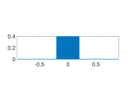
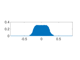
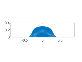
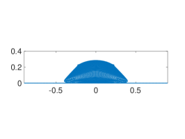
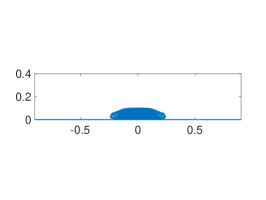
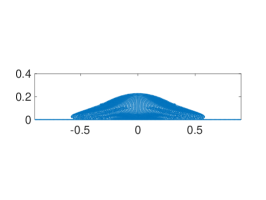
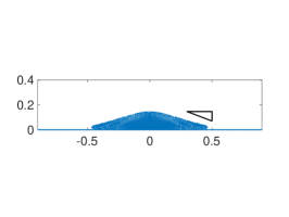
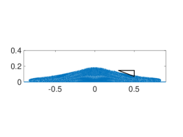
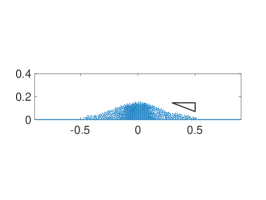
We considered a two dimensional collapsing column of sand as shown in Fig. 1, where the sand has initial width $2L_{0}$ and height $H_{0}$. The aspect ratio is defined as $a=H_{0}/L_{0}$. In our numerical experiments, we have used different aspect rations keeping $L_{0}$ constant and varying $H_{0}$.

Figure 1: Initial geometry of a sand column of height $H_{0}$ and width $2L_{0}$.

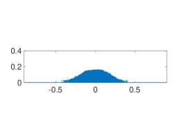
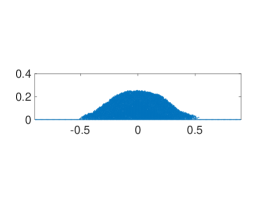
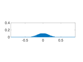
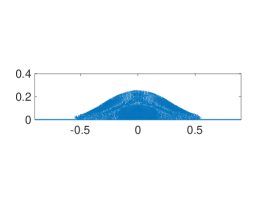
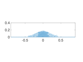
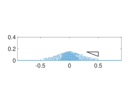
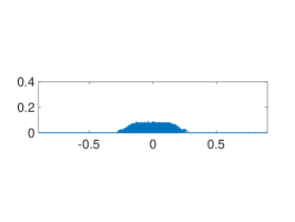
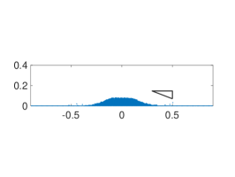
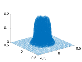
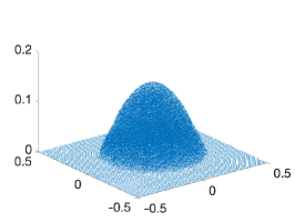
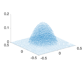
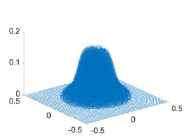
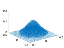
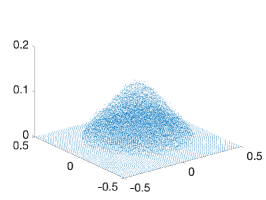
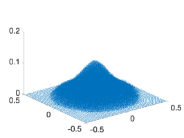
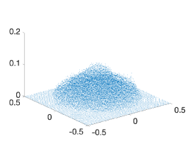
For the first numerical experiment we fix all parameters to the values given above. We determine first the results of the microscopic model (Section 4) with $N=2000$. Then, the results of a well resolved simulation using the plasticity model (Section 2) and the simplified model (Section 3) with $N=2000$ grid particles are computed. In Figures 2 – 5 we have plotted the results obtained from these three models at times $t=0.0,0.2,0.3,0.5$. One observes a good coincidence between microscopic and plasticity model with some discrepancies for the initial stages of the evolution. The simplified Coulomb constitutive model deviates further from the microscopic model.

Figure 2: Initial values for $a=0.5$ (left), $a=1$ ( middle), $a=2$ (right) at $t=0$.

Figure 3: Time development at $t=0.2$ for $a=0.5$ (left), $a=1$ ( middle), $a=2$ (right). First row: micoscopic model (Section 4), second row: plasticity model (Section 2),third row: Coloumb constitutive model (Section 3)

Figure 4: Time development at $t=0.3$ for $a=0.5$ (left), $a=1$ ( middle), $a=2$ (right). First row: micoscopic model (Section 4), second row: plasticity model (Section 2),third row: Coloumb constitutive model (Section 3)

Figure 5: Time development at $t=0.5$ for $a=0.5$ (left), $a=1$ ( middle), $a=2$ (right). First row: micoscopic model (Section 4), second row: plasticity model (Section 2),third row: Coloumb constitutive model (Section 3)

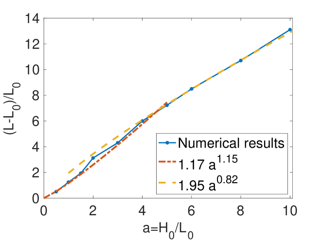
In Fig. 6 we have plotted the non-dimensional run out distance against the aspect ratio $a$. They are similar for all models. We observed that for smaller values of aspect ratio $a$ a good approximation is given by $\frac{L-L_{0}}{L_{0}}=1.17a^{1.15}.$ For larger values of $a$ a good approximation is given by $1.95^{0.82}.$ Such values are consistent with numerical and experimental results discussed, for example, in [18].

Figure 6: Non-dimensional run-out distance vs non-dimensional aspect ratio $a=H_{0}/L_{0}$.

Additionally, we have investigated the dependence of the results on the number of microscopic and macroscopic grid particles used. In Figure 7 we have plotted the results of the plasticity model with a number of particles $N=2000,1000,500$ leading all to comparable solutions. Similarly in Figure 8 the results of the microscopic equations are obtained for $N=2000$ and $N=1000$ particles. In Figure 9 the results of the simplified macroscopic equations are obtained for $N=2000$ and $N=1000$ particles. Plotting times are $t=0.2,0.3,0.5$ in all cases.

Note that the constant time step $\Delta t=10^{-5}s$ is used for the microscopic model and the macroscopic plasticity model with $N=2000$. For $N=500$ a smaller time step still gives stable solutions. We use $\Delta t=2\cdot 10^{-5}s$. In case of the simplified Coulomb constitutive model a larger times step can be used due to the implicit time discretization.

From Figures 7 and 8 one observes that the macroscopic plasticity model gives accurate results also for a number of particles as small as $N=500$. The results of the microscopic model strongly diverge for $N=1000$ from the ones obtained from $N=2000$ particles. In case of the simplified macroscopic models one obtains a behaviour results, which is rather similar to the behaviour of a viscous fluid.

The simulations is performed in MacOS Monterey Version $12.5$ with processor $3.4$ GHz Quad-Core Intel Core i5, memory $16$ GB $2400$ MHz DDR4, where a single processor is used. The CPU time for the macroscopic plasticity simulation with $N=2000$ is about $36$ and for $N=500$ about $4$ minutes. The CPU time for the microscopic simulation with $N=2000$ is around $7$ minutes. Thus, using the macroscopic model with $N=500$ yields a gain of approximately a factor of $2$ compared to the computation times of the microscopic model with $N=2000$.

We note that in case of the simplified mode, due to the possibility of using a smaller time step, the required computation time for $N=2000$ is an order of magnitude smaller than for the microscopic model.

Figure 7: Time development of the solution of plasticity model for $a=1$ at times $t=0.2,0.3,0.5$ (from top row to bottom row). First column: $N=2000$, second column: $N=1000$, third column: $N=500$.

.

Figure 8: Time development of the microscopic solution for $a=1$ at times $t=0.2,0.3,0.5$ from left to right. First row: $N=2000$, second row: $N=1000$.

.

Figure 9: Time development of the solutions of Coloumb constitutive model for $a=1$ at times $t=0.2,0.3,0.5$ from left to right. First row: $N=2000$, second row: $N=1000$.

.

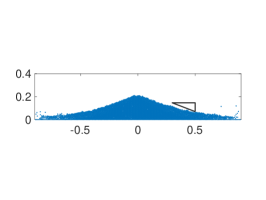
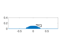
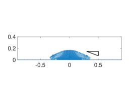
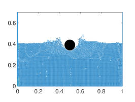
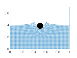
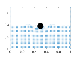
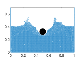
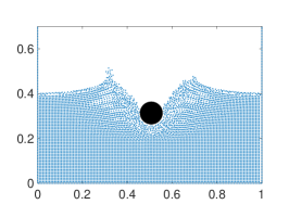
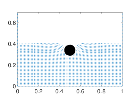
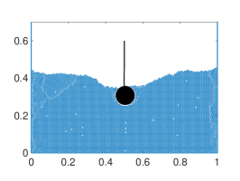
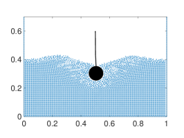
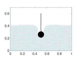
6.3 Free falling disc in a $2D$ sand box

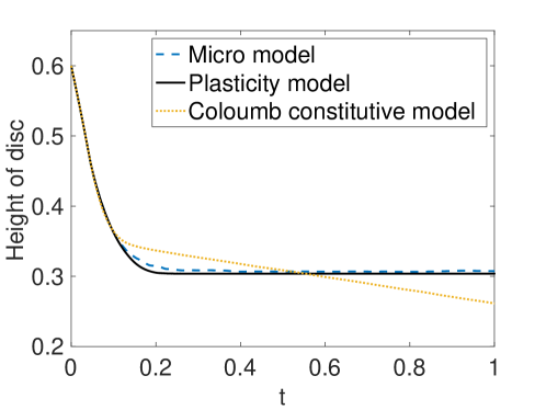
In this subsection we present the simulation of a falling disc into a box filled with sand. Consider a box of size $[0,1]m\times[0,1]m$ with the sand initially filled up to the height $y=0.4m$. We consider a case, where a disc of radius $0.05m$ located in the center of the box falls from the height $y=1m$. For the numerical simulation, initally, the center of the disc is located at $(0.5,0.6)$ and the initial velocity of the disc is equal to $\sqrt{2g0.4}=2.8014m/s$, where $g=9.81m/{s^{2}}$. The density of the disc is $8050kg/{m^{3}}$. The other parameters are the same as in the collapsing column case. The time step is chosen as $\Delta t=5\cdot 10^{-6}.$ In figure 10 we have plotted the positions of sand particles and disc computed from the microscopic, the plasticity and the simplified model at time $0.08s,0.16s$ and $1s$. The microscopic model is simulated with $10890$ particles and plasticity and simplified models are simulated with initially $2420$ grid points. Figure 11 shows the height of the discs versus time. As can be seen in Figure 10 and Figure 11, the solutions obtained from microscopic and plasticity models are very close, however, the solution obtained from the simplified model deviates strongly in this case being similiar to a highly viscous flow solution.

Figure 10: Comparison of the stationary solutions of the microscopic model (left) plasticity model (middle) and simplified model (right) solutions. The first row is at time $t=0.08s$, second row at $t=0.16s$ and the third row is at $t=1s$ seconds.

Figure 11: Comparison of the height of the disc with respect to time

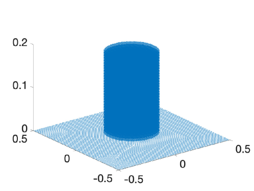
6.4 Collapsing $3D$ sand column

In this subsection we consider a collapsing 3 dimensional sand pile.We have considered a cylindrical sand pile of radius 0.2 with height 0.2. The parameters are the same as in the $2D$ case. Like in the $2D$ case we have plotted in Fig. 13 the sand position at $t=0.2,0.3,0.5$ obtained from macroscopic plasticity model and from microscopic model. The CPU times for microscopic and plasticity models are compared up to the final simulation time $t=0.5$. For the microscopic model, the total number of particles is $153317$ with interior and boundary particles are $121905$ and $31412$, respectively. The time step for the microscopic model is $\Delta t=2\times 10^{-5}$ is considered. The CPU time for the microscopic model is $8$ hours. In the case of the plasticity model, we have used different resolutions with a maximal number of particles $128105$ including $111360$ interior and $16745$ boundary particles. The time step for this resolution is $\Delta t=10^{-5}$. The CPU time for such a simulation is $38$ hours. However, using the macroscopic plasticity model one can obtain the same results with a much coarser resolution. For example, we have considered the total number of particles $24624$ with $19440$ interior and $5184$ boundary particles. Again, the time step is $\Delta t=2\times 10^{-5}$. In this case the CPU time is only $3$ hours, which is considerably smaller than in the microscopic case. The results are plotted in Fig. 12, where the first column shows the results from the microscopic model, the second column the ones from the plasticity model with the fine resolution and the third column shows again the plasticity model, but this time with the coarse resolution. The time evolutions of $2D$ and $3D$ columns of microscopic and macroscopic models are similar. In the early stage, for example, at times $t=0.2$ and $0.3$ the sand column obtained from the microscopic model differs from the macroscopic model, where as in the stationary case, they have very good agreements.

Figure 12: Initial cylindrical sand column.

Figure 13: Time development of the microscopic model with $153317$ particles (left) and plasticity model with 128105 sand particles (middle) and 24624 sand particles (right) at times $t=0.2,0.30.5$ (from top to bottom).

7 Conclusion

This work shows the results of an implementation of the elasto-viscoplastic model developed in [18] in the framework of a GFDM particle method. The case of a collapsing sand column and of a sphere falling into a box filled with sand has been considered. Moreover, a comparison with a microscopic model of nonlinear Hertz type with parameters, which are physically consistent with those of the macroscopic model, is presented in both cases, showing very good coincidence of the two approaches. Additionally a simplified model based on the $\mu(I)$ rheology in the framework of incompressible balance equations is investigated.

In particular, for the case of the falling disc advantages of the approach in [18] compared to a simplified use of the $\mu(I)$ rheology in the framework of incompressible balance equations are clearly observed. Concerning the computational times required for the simulations, the results for the collapsing sand columns shows, that the number of particles can be considerably reduced in the case of the macroscopic plasticity model compared to the microscopic model. This leads to a reduction in CPU times between microscopic and macroscopic simualtions by a factor of 3.

Acknowledgments

This work is supported by the BMBF-Program ’Mathematik für Innovationen’, Project HYDAMO and by the DFG (German research foundation) under Grant No. KL 1105/30-1.

References

- [1] P. Cundall, O.D. Strack, A discrete numerical model for granular assemblies, Geotechnique, 29, 47-65, 1979.
- [2] F. Da Cruz, S. Emam, M. Prochnow, J. Roux, F. Chevoir, Rheophysics of dense granular materials:discrete simulation of plane shear flows, Phys. Rev. E, 72, 021305, 2005.
- [3] G. Daviet, F. Bertails-Descoubes, A semi-implicit material point method for the continuum simulation of granular materials, A CM transactions on graphics, SIGGRAPG 16, Technical papers, 35, 102:1-13, 2016.
- [4] I. Ostermann, J. Kuhnert, D. Kolymbas, C.-H. Chen, I. Polymerou, V. Šmilauer, C. Vrettos, D. Chen, Meshfree generalized finite difference methods in soil mechanics, Int J Geomath., 2013.
- [5] D. Liu, D.L.Henann, Non-local continuum modelling of steady, dense granular heap flow, J. Fuid Mech., 831, 212-227, 2017.
- [6] R. Narain, A. Golas, M. C. Lin, Free-Flowing Granular Materials with Two-Way Solid Coupling, in ACM SIGGRAPH Asia 2010 Papers, SIGGRAPH ASIA ’10, Association for Computing Machinery, New York, USA, 2010.
- [7] M. Laetzel, S. Luding, H. J. Herrmann, Macroscopic material properties from quasi-static, microscopic simulations of a two-dimensional shear-cell, Granular Matter, 2, 123-135, 2000.
- [8] J. Schaefer, S. Dippel, D. Wolf, Force Schemes in Simulations of Granular Materials, Journal de Physique I, 6, 5-20, 1996.
- [9] K. Kamrin, Nonlinear elasto-plastic model for dense granular flow, International Journal of Plasticity, 26(2), 167-188, 2010.
- [10] D.G. Schaeffer, Instability in the Evolution Equations Describing Incompressible Granular Flow, J. Diff. Eq., 66, 19-50, 1987.
- [11] T. Barker, D.G. Schaeffer, M. Shearer, J.M.N.T. Gray, Well-posed continuum equations for granular flow with compressibility and -rheology, Proc. R. Soc. A, 473, 20160846, 2017.
- [12] C.M. Mast, P. Arduino, P. Mackenzie-Helnwein, G. R. Miller, Simulating granular column collapse using the Material Point Method, Acta Geotechnica, 10, 101-116, 2010.
- [13] S. J. Cummins, J. U. Brackbill, An Implicit Particle-in-Cell Method for Granular Materials, J. Comput. Phys., 180, 506-548, 2002.
- [14] P. Jop, Y. Forterre, O. Pouliquen, Crucial role of sidewalls in granular surface flows: consequences for the rheology, J. Fluid Mech., 541, 167-192, 2005.
- [15] P. Jop, Y. Forterre, O. Pouliquen, A constitutive law for dense granular flows, Nature letters, 441, 04801, 2006.
- [16] P.-Y. Lagree, L. Staron, S. Popinet, The granular column collapse as a continuum: validity of a two-dimensional Navier-Stokes model with a -rheology, J. Fluid Mech., 686, 378-408, 2011.
- [17] L. Lacaze, J. C. Phillips, R. R. Kerswell, Planar collapse of a granular column: Experiments and discrete element simulations, Phys. Fluids, 20, 063302, 2008.
- [18] S. Dunatunga, K. Kamrin, Continuum modelling and simulation of granular flows through their many phases, J. Fluid Mech., 779, 483-513, 2015.
- [19] C. Drumm, S. Tiwari, J. Kuhnert, H.-J. Bart, Finite pointset method for simulation of the liquid–liquid flow field in an extractor, Computers & Chemical Engineering, 32(12), 2946-2957, 2008.
- [20] S. Tiwari, J. Kuhnert, Modelling of two-phase flow with surface tension by Finite Point-set method (FPM), J. Comp. Appl. Math., 203, 376-386, 2007.
- [21] P. Suchde, J. Kuhnert, S. Tiwari, On meshfree GFDM solvers for the incompressible Navier-Stokes equations, Computers and Fluids, 165, 1-12, 2018.
- [22] S. Tiwari, A. Klar, S. Hardt, Numerical simulation of wetting phenomena by a meshfree particle method, J. Comput. Appl. Math., 292, 467-485, 2016.
- [23] S. Tiwari, A. Klar, G. Russo, A meshfree arbitrary Lagrangian-Eulerian method for the BGK model of the Boltzmann equation with moving boundaries, J. Comput. Phys., 458, 111088, 2022.