Modeling and Analysis of Satellite Constellation Leveraging Cox Point Processes

A Novel Analytical Model for LEO Satellite Constellations Leveraging Cox Point Processes

Abstract

This work develops an analytical framework for downlink Low Earth Orbit (LEO) satellite communications, leveraging tools from stochastic geometry. We propose a tractable approach to the analysis of such satellite communication systems, accounting for the fact that satellites are located on circular orbits. We accurately incorporate this geometric property of LEO satellite constellations by developing a Cox point process model that jointly produces orbits and satellites on these orbits. Our work contrasts with previous modeling studies that presumed satellite locations to be entirely random, thereby overlooking the fundamental fact that satellites are exclusively positioned on orbits. Employing this new Cox model, we analyze the network performance experienced by users anywhere on Earth. Specifically, we evaluate the no-satellite probability of the proposed network and the signal-to-interference-plus-noise ratio (SINR) distribution, or the coverage probability. By presenting fundamental network performance as functions of network key parameters, this work allows one to assess the statistical properties of downlink LEO satellite communications and can thus be used as a system-level design tool to operate, design, and optimize forthcoming complex LEO satellite networks.

I Introduction

I-A Motivation and Related Work

Satellite communications provide global-scale connectivity to users everywhere on earth without the need for deploying base stations and infrastructure on the ground [1, 2]. As orbiting the earth at very high speeds, LEO satellites provide reliable and fast Internet connectivity to millions of devices [1, 2]. In the early stage of satellite communications, the number of deployed satellites was very small, and thus only a limited number of satellites were available for connections. For instance, the Iridium constellation [3]—6 orbits with 11 satellites each orbit—provided a call coverage of up to 7 minutes. Because of the motion of satellites and their limited number, the call was either dropped or transferred after about 7 minutes. Preventing outages was one of the key design criteria for satellite communications of this early stage.

In modern LEO satellite communication systems with many LEO satellites, the goal is not only to prevent call outages but also to provide high-speed and low-latency Internet connections to millions of devices. Leveraging a large number of satellites, often integrated with terrestrial network infrastructures [4, 5], LEO satellite communication systems are envisioned to handle various demands of ground or even aerial devices around the globe. Recent, several companies intend to establish their LEO satellite communication networks by building such large constellations for global connectivity [6, 7, 8]. It is not hard to imagine a large number of LEO satellites from various companies will provide Internet connections to devices anywhere on earth. Since the spatial distribution of LEO satellites determines the performance of communications on LEO satellite networks, building an analytical framework is vital to the description and analysis of the LEO satellite communications.

To provide an analytical framework for describing the locations of LEO satellites, several recent papers [9, 10, 11, 12, 13, 14] used stochastic geometry [15, 16, 17]. This stochastic geometry approach has been shown to be useful in the modeling of cellular and vehicular networks because it not only provided geometric treatment to the interference and coverage in such networks but also identified key network performance behaviors as functions of networks’ distributional parameters [18, 19, 20, 21]. Similarly, in the context of LEO satellite modeling, [9, 10, 11, 12, 13, 14] modeled the distribution of satellites as binomial or Poisson point processes [15, 16], where the satellites’ locations are assumed to be uniformly distributed on a sphere. In contrast to [9, 10, 11, 12, 13], the impact of interference created by a binomial satellite point process was evaluated and accounted for the SINR coverage probability in [14]. It is important to note that the recent modeling technique based on binomial or Poisson point processes [9, 10, 11, 12, 13, 14] overlooked the essential geometric facts that LEO satellite constellations are comprised of orbits and that LEO satellites are on these orbits. Therefore, the consequences of such geometric characteristic cannot be investigated. This motivates us to develop an isotropic Cox point process model that incorporates these geometric characteristics. This process jointly produces orbits and LEO satellites on these orbits, isotropically distributed in space. Adhering to the fundamental geometric observation that LEO satellites are on their orbits, our developed isotropic Cox model allows us to analyze the network performance seen by users anywhere on Earth. To the best of our knowledge, this is the first work that explicitly models the orbits and LEO satellites on them and analyzes the typical network performance of downlink communications from LEO satellites to network users anywhere on Earth. To demonstrate the use of the developed analytical framework, we derive the no-satellite probability and then the coverage probability of downlink communication from LEO satellite to a typical user. To illustrate the applicability of the model, we conduct numerical experiments showing that our Cox model adequately represents the local properties of forthcoming LEO satellite constellations.

I-B Theoretical Contributions

Novel modeling technique for satellite constellations: This work develops an analytical framework for LEO satellite networks using stochastic geometry. Specifically, we develop a Cox model that jointly produces orbits and satellites on them, ensuring that these LEO satellites always follow their orbital trajectories. The proposed Cox model for LEO satellites stands in contrast to most existing frameworks that have adapted binomial point processes to describe the locations of satellites as random points. While a recent work shows that the binomial point process model may locally portray some existing satellite constellations to some extent [22], it fails to capture the geometric fact that satellites are always located on orbits, which significantly affects network geometry. By incorporating this crucial geometric attribute prevalent in most LEO satellite networks, our developed framework serves as one of several modeling techniques for LEO satellite networks. Section VI demonstrates the application of our newly developed Cox point process in modeling upcoming constellations. Then, we also show that our Cox point process model is versatile enough to reproduce the network performance of the network modeled by a binomial point process only by simply adjusting its scale parameters.

Analysis of downlink LEO satellite communications: First, we prove that our developed Cox point process is isotropic, namely invariant by all rotations. Leveraging this rotation invariance property, we derive a closed-form expression for the arc length of an orbit and provide an integral formula for the distribution of the distance from a typical user to its nearest LEO satellite. These values are essential in the derivation of the network performance of the LEO satellite network seen by the typical user. For example, leveraging this, we derive the probability that a typical user has no visible satellite as a function of the density of orbits $\lambda$, the density of satellites per orbit $\mu,$ and the satellite altitude $r_{a}$. Further, given that a LEO satellite constellation not only provides downlink signals but also creates unwanted interference, we study the performance of LEO downlink communication systems through the SINR distribution of the typical user. Assuming Nakagami-$m$ fading, we derive the coverage probability of the typical user for this generic fading scenario. We compare the derived coverage formula to the results obtained by Monte Carlo simulations and we validate the accuracy of the derived formula.

Design insights applicable to practical LEO satellite network: Our approach provides a comprehensive tool for designing and enhancing LEO satellite communication systems. For example, we derive an expression for the interference experienced by the typical user, which is a function of the orbit density $\lambda$ and the satellite density per orbit $\mu$. This expression can be utilized to design interference management techniques in densely-deployed LEO satellite communication systems, taking into account the number of orbital planes and interfering satellites. Additionally, this paper obtains expressions for the no-satellite probability and the coverage probability as the functions of $\lambda$ and $\mu$, enabling the assessment of each variable’s individual impact on the system’s large-scale performance metrics. Without time-consuming system-level simulation with large number of LEO satellites and their users on earth, network operators of LEO satellite systems can explore various deployment options by controlling the number of satellites per orbit or the number of orbits per altitude, considering different deployment strategies through variations in network variables such as $\lambda$, $\mu,$ or $r_{s}$. Lastly, the proposed model and analysis could serve as a basis for assessing the time-domain performance metrics of LEO satellite networks, such as the time fraction of coverage or the association delay distribution.

II System Model

II-A Models for Orbits and Satellites

We denote by $r_{e}$ the radius of Earth ($r_{e}\approxeq 6400$ km) and the center of Earth is located at the origin of the Euclidean space. The reference plane is the $xy$ plane and the longitudinal zero point is the $x$-axis. We denote by $r_{a}$ the altitude of the satellites or equivalently the radius of orbits. All orbits are assumed to be circles centered at the origin. Let $r_{s}=r_{e}+r_{a},$ where $r_{s}$ is the radius of orbits.

Figure 1: Let $A$ be the ascending point. The longitude $\theta$ is the angle that $\overline{OA}$ makes with the $x$-axis. The inclination $\phi$ is the angle that the orbital plane makes with the reference plane. $\omega$ is the angle that the $\overline{OX}$ makes with $\overline{OA}.$

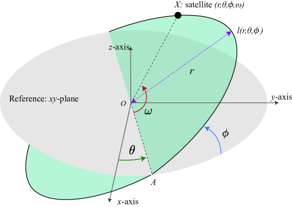
To model circular orbits of LEO satellites in the simplest case, we first consider a Poisson point process $\Xi$ of density $\lambda\sin(\phi)/(2\pi)$ on the rectangle set $\operatorname{\mathcal{R}}{=}[0,\pi)\times[0,{\pi})$. We write $\Xi=\sum_{i}\delta_{(\theta_{i},\phi_{i})}$. Each point of the Poisson point process on $\operatorname{\mathcal{R}}$, say $(\theta,\phi)$, is mapped to an undirected orbit $l(\theta,\phi)$ in the Euclidean space $\operatorname{\mathbb{R}}^{3}$. Specifically, $\theta$ is the longitude and $\phi$ is the inclination. See Fig. 1. The orbit process $\operatorname{\mathcal{O}}$ on $\operatorname{\mathbb{R}}^{3}$ is

$$\operatorname{\mathcal{O}}=\bigcup_{i\in\operatorname{\mathbb{Z}}}l(\theta_{i},\phi_{i})=\!\!\bigcup_{{(\theta_{i},\phi_{i})}\in\Xi}\!\!l(\theta_{i},\phi_{i}).$$ (1)

The orbit process is a union of circles located on the sphere $\operatorname{\mathbb{S}}_{r_{s}}{=}\{(x,y,z)|x^{2}+y^{2}+z^{2}=r_{s}^{2}\}$. Since the density of the Poisson point process $\Xi$ is $\lambda\sin(\phi)/(2\pi)$, there are $\lambda$ points on $\operatorname{\mathcal{R}}$ on average, or equivalently, there are $\lambda$ orbits on $\operatorname{\mathbb{R}}^{3}$ on average. The orbit process $\operatorname{\mathcal{O}}$ is isotropic, namely rotation invariant. We will shortly prove its rotation invariance property in Section III.

To represent the locations of satellites on orbits, we leverage the conditional structure based on a Cox point process. Specifically, conditionally on each orbit $l(\theta_{i},\phi_{i})$, the satellites on each orbit are modeled as a Poisson point process $\psi_{i}$ of mean $\mu$. Because of the conditional structure, our developed LEO satellite model geometrically ensures that the satellites are exclusively on orbits given by $\operatorname{\mathcal{O}}$. Based on the above construction, the orbital angles $\omega$ of satellites (See. Fig. 1.) are also characterized as a Poisson point process of intensity $\mu/(2\pi)$ on the finite interval $[0,2\pi).$

Collectively, the satellite point process $\Psi$ on $\operatorname{\mathbb{R}}^{3}$ is $\Psi=\sum_{i\in\operatorname{\mathbb{Z}}}\psi_{i}.$ The satellite point process is defined conditionally on the orbit process and it is hence a Cox point process [15, 16].

It is worth noting that the conditional structure of Cox point process was found to be useful in the modeling of vehicular networks on two-dimensional $\operatorname{\mathbb{R}}^{2}$ plane since it jointly creates road systems and vehicles on them [23, 24, 20]. In the same way as vehicles are on roads in two-dimensional vehicular networks, satellites are on orbits in three-dimensional LEO satellite networks.

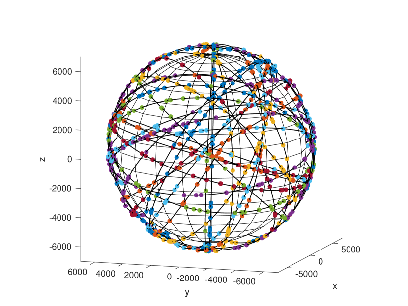
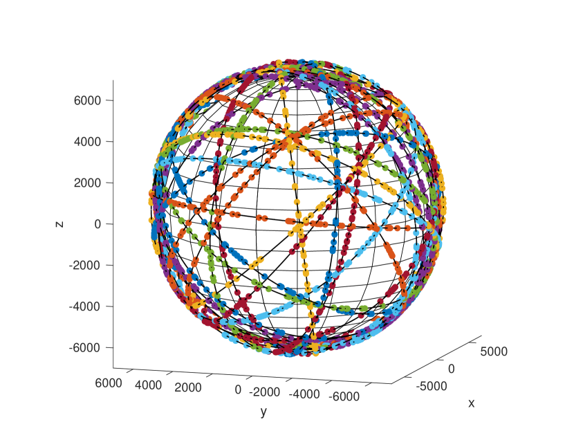
Figs. 2 – 3 illustrate the proposed network model with various $\lambda$ and $\mu$ parameters. The proposed stochastic geometry framework of populating orbits and their corresponding satellites is designed to easily change the number of satellites, the number of orbits, or their topological characteristics. For instance, we may increase the total number of satellites by individually increasing $\lambda$ or $\mu$ or both. Fig. 3 shows $\mu=120$ and since satellites are densely populated on the finite orbital planes, the clustering of the LEO satellites on their orbits are more pronounced.

Figure 2: The proposed model with $\lambda=30$, $\mu=40$, and $r_{s}=7000\text{ km}$.

Figure 3: The proposed model with $\lambda=28$, $\mu=120$, and $r_{s}=7000\text{ km}$.

II-B User Location

To reduce the computational complexity accompanied with the distribution of users, we begin with the simplest assumption that users are uniformly distributed on Earth. For the ease of analysis, this user assumption was extensively used also in [9, 10, 11, 12, 13, 14]. More precisely, the network users are modeled as a Poisson point process of intensity $\lambda_{u}/(4\pi^{2}r_{e}^{2})$ on the sphere $\{(x,y,z)\in\operatorname{\mathbb{R}}^{3}|x^{2}+y^{2}+z^{2}=r_{e}^{2}\}$. Here, $\lambda_{u}$ is the average number of network users in the system. We also assume that users and LEO satellites are independent. For downlink communications, users are assumed to get their downlink signals from their closest LEO satellites [25, 9, 10, 11, 12, 13, 14]. The distribution of network users and their downlink association play an important role in determining the fundamental performance of downlink LEO satellite communication systems.

II-C Propagation Model

The downlink signals from LEO satellites attenuate because of Doppler shift, weather, rain, reflection from objects, and path loss over the space. In practice, Doppler shift can be compensated by exploiting the existing data on satellites’ orbits and speeds [26, 27]. A few large-scale uniform factors such as rain attenuation can be ignored under certain conditions [27, 11, 12, 13]. To emphasize the role of satellite geometry onto the network performance, we propose a simple propagation model where various attenuating and propagation factors are assumed to be aggregated to a single independent fading random variable. This approach was found useful in recent work [11, 12, 13], where analytical tractability was achieved by focusing on the impact of topology of LEO satellite communication systems.

Suppose a transmitter and a user separated by a distance $d.$ Assume the transmitter is visible to the user. We assume that the received signal power at the user is then given by

$$pG_{1}(\zeta)G_{2}(\zeta)Hd^{-\alpha},$$ (2)

where $p$ is the LEO satellite transmit power, $G_{1}(\zeta)$ is the antenna gain of the LEO satellites, $G_{2}(\zeta)$ is the antenna gain employed by network users, $H$ is a random variable representing small-scale fading, and $\alpha$ is the path loss exponent.

To make the analysis tractable, we assume that network users and satellites are able to direct their antennas toward their associated counterparts by using technologies such as phased antenna array [28, 13]. We assume that the gain $G_{1}(\zeta)$ of the LEO satellites is

$$G_{1}(\zeta)=\begin{cases}g&|\zeta|<\zeta_{t},\\ 1&|\zeta|>\zeta_{t},\end{cases}$$ (3)

where $\zeta$ is the boresight angle from the antenna’s maximum radiated power direction. Similarly, as in [29, 13], network users are assumed to be equipped with isotropic antennas $G_{2}(\zeta)=g_{r}$.

To encompass general fading cases, we use a Nakagami-$m$ fading [14]. The CCDF of the random variable ${H}$ in Eq. (2) is hence given by

$$\operatorname{\mathbf{P}}(H>x) =e^{-mx}\sum\limits_{k=0}^{m-1}\frac{(mx)^{k}}{k!} \forall x\geq 0,$$

where $m\geq 1$. When $m=1$, Nakagami-$m$ fading becomes Rayleigh fading and $H$ becomes an exponential random variable with mean one.

II-D Performance Metrics

A downlink LEO satellite communication system is built to cover all network users. Nevertheless, some users on the surface of the earth may not be well covered because of the lack of visible satellite or weak signals.

We define the no-satellite event as the event that there is no visible satellite from a network user. Since the Earth rotates and the relative locations of LEO satellites vary over time, we characterize this through the no-satellite probability.

To evaluate the basic performance of downlink LEO satellite communication systems, we study the coverage probability, namely the SINR distribution of network users. The coverage probability incorporates the path loss, the topological properties of the association satellite and of the interfering satellites, the small-scale fading, the antenna gains, and the background thermal noise. The coverage probability of a user at an arbitrary location $y$, or equivalently the CCDF of SINR at user $y$, is given by

$$\operatorname{\mathbf{P}}(\operatorname{\textnormal{SINR}}_{y}>\tau)$$

$$=\operatorname{\mathbf{P}}_{y}\left(\frac{pG_{X_{y};y}H_{i}\|X_{y}-y\|^{\alpha}}{\sigma^{2}+\sum_{X_{j}\in\bar{\Psi}\setminus X_{y}}pG_{X_{j};y}H\|X_{j}-y\|^{\alpha}}>\tau\right)$$

$$=\operatorname{\mathbf{P}}_{y}\left(\frac{pgH_{i}\|X_{y}-y\|^{\alpha}}{\sigma^{2}+\sum_{X_{j}\in\bar{\Psi}\setminus X_{y}}pH_{j}\|X_{j}-y\|^{\alpha}}>\tau\right),$$ (4)

where $X_{y}$ is the location of the satellite that serves the user at $y$, $G_{X_{i};y}$ is the aggregate antenna gain from the satellite at $X_{i}$ toward the user at $y$, $\sigma^{2}$ is the noise power, and $\bar{\Psi}_{y}$ is the point process of satellites visible at $y$. We define $G_{X_{y};y}=gg_{r}$ and $G_{X_{j};y}=g_{r}\ \forall X_{j}\neq X_{y}$. We use subscripts to distinguish satellites’ locations and small-scale fading associated with them. The constant $\tau$ is the SINR threshold.

III Statistics of Orbits and Satellites

This section provides statistical properties of the proposed satellite Cox point process that are essential to the analysis of the downlink communications from satellites to users.

III-A Isotropy

Theorem 1.

$\mathcal{O}$ and $\Psi$ are isotropic, namely invariant by all rotations.

Proof:

Below, the reference basis of $\mathbb{R}^{3}$ is denoted by $(e_{x},e_{y},e_{z})$ and the unit sphere of center $o=(0,0,0)$ in $\mathbb{R}^{3}$ is denoted by $\operatorname{\mathbb{S}}$. Let $U$ be a uniformly distributed random point on $\operatorname{\mathbb{S}}$. For each ${U}$, there is a unique directed orbit $\operatorname{\mathcal{O}}(U)\subset\operatorname{\mathbb{S}}$, which is the orbit whose normal vector is $\overrightarrow{oU}$ with a direction that is the trigonometric (counterclockwise) direction with respect to (w.r.t.) this vector (namely seen from point $U$). Note that $\operatorname{\mathcal{O}}(U)$ is a factor of ${U}$; namely, for all $\operatorname{\mathbb{R}}^{3}$ rotations $R$ of center $o$, the orbit $\operatorname{\mathcal{O}}(R(U))$ coincides with the orbit $R(\operatorname{\mathcal{O}}(U))$. Since the law of $U$ is isotropic on $\operatorname{\mathbb{S}}$ (namely left invariant by all $R$), it follows from the relation $\operatorname{\mathcal{O}}(R(U))=R(\operatorname{\mathcal{O}}(U))$ that the law of $\operatorname{\mathcal{O}}(U)$ is also isotropic.

It is well known [30] that the uniform random vector ${U}$ can be represented as

$${U}=(\sqrt{1-V^{2}}\cos(\Theta),\sqrt{1-V^{2}}\sin(\Theta),V),$$ (5)

in the basis $(e_{x},e_{y},e_{z})$ where $V\sim\text{Uniform}(-1,1)$, $\theta\sim\text{Uniform}(0,2\pi),$ and $V\mathchoice{\mathrel{\hbox to0.0pt{$\displaystyle\perp$\hss}\mkern 2.0mu{\displaystyle\perp}}}{\mathrel{\hbox to0.0pt{$\textstyle\perp$\hss}\mkern 2.0mu{\textstyle\perp}}}{\mathrel{\hbox to0.0pt{$\scriptstyle\perp$\hss}\mkern 2.0mu{\scriptstyle\perp}}}{\mathrel{\hbox to0.0pt{$\scriptscriptstyle\perp$\hss}\mkern 2.0mu{\scriptscriptstyle\perp}}}\Theta.$

For the directed orbit $\operatorname{\mathcal{O}}(U)$, we define

• The longitude angle $\theta\in[0,2\pi)$ to be the angle $\angle{e_{x}}\overrightarrow{oA}$, where $A$ is the ascending point of the orbit on the $xy$-plane;

• The inclination angle $\phi\in[0,\pi)$ to be the angle $\angle{}e_{z}\overrightarrow{oU}$.

It follows from Eq (5) that we can represent the longitude and inclination as follows:

$$\theta =\Theta+\pi/2\mod 2\pi,$$ (6)

$$\phi =\arccos(V).$$ (7)

Since $V$ and $\Theta$ are independent random variables, we have that $\phi$ and $\theta$ are independent. In other words, the longitude and inclination of the orbit are independent. Furthermore, since $\Theta\sim\text{Uniform}[0,2\pi)$, we also have $\theta\sim\text{Uniform}[0,2\pi)$. Then, based on the fact that $V\sim\text{Uniform}[-1,1)$, we arrive at

$${\mathbb{P}}(\phi<x)={\mathbb{P}}(V<\cos(x))=\frac{1-\cos(x)}{2},\quad\quad 0\leq x<\pi.$$

Using the above CDF, we get the PDF of $\phi$ as follows:

$$f_{\phi}(x)=\begin{cases}\frac{\sin(x)}{2},&\text{for }0\leq x<\pi,\\ 0&\text{otherwise}.\end{cases}$$ (8)

The isotropic directed orbit Poisson point process can hence be represented as a Poisson point process of density

$$\Lambda(\phi,\theta)=\frac{\lambda}{4\pi}\sin(\phi),$$ (9)

on the rectangle set $\mathcal{R}=[0,\pi)\times[0,2\pi)$. Here, $\lambda$ corresponds to the mean number of directed orbits.

Furthermore, the directed orbit with angles $(\theta,\phi)$ and that with angles $(\theta+\pi,\phi+\pi/2\mod\pi)$ reduce to the same orbit when forgetting the orbit direction. Therefore, for an undirected isotropic orbit, its longitude angle $\widetilde{\theta}$ is defined as the angle that the orbital plane makes with the reference plane in $[0,\pi)$ and it is uniformly distributed in this interval.

Based on the same principle, the isotropic undirected orbit Poisson point process can hence be represented as a Poisson point process of density

$$\widetilde{\Lambda}(\widetilde{\phi},\widetilde{\theta})=\frac{\widetilde{\lambda}}{2\pi}\sin(\widetilde{\phi}),$$ (10)

on the rectangle set $\widetilde{\mathcal{R}}=[0,\pi]\times[0,\pi]$. Here, $\widetilde{\lambda}$ is the mean number of undirected orbits.

Since the density of the orbit process is given by Eq. (10), the proposed orbit process is isotropic. Furthermore, conditionally on each orbit, the satellite point process on each orbit is isotropic. As a result, the Satellite Cox point process is isotropic. ∎

Remark 1.

Note that this isotropic property also appears in recent work [9, 10, 11, 12, 13, 14] where binomial or Poisson point processes were used to model the distribution of LEO satellites. Those isotropic models are capable of effectively depicting the local geometry of real LEO satellite deployment scenarios, by using intensity parameters obtained from such scenarios. Similarly, our developed framework is also capable of incorporating the local geometry of LEO satellite distribution and analyzing the downlink communications therein, by obtaining the mean number of orbits and the mean number of satellites out of real scenarios and then by applying them to the analysis. See Section VI.

Lemma 1.

The average number of all satellites is $\lambda\mu.$

Proof:

The average number of satellites is given by

$$\operatorname{\mathbf{E}}[\Psi] \stackrel{{\scriptstyle(\text{a})}}{{=}}\operatorname{\mathbf{E}}\left[\sum_{l(\theta_{i},\phi_{i})\in\operatorname{\mathcal{O}}}\sum_{X_{j}\in\psi_{i}}1\right]$$

$$\stackrel{{\scriptstyle(\text{b})}}{{=}}\operatorname{\mathbf{E}}\left[\sum_{l(\theta_{i},\phi_{i})\in\operatorname{\mathcal{O}}}\operatorname{\mathbf{E}}\left[\left.\sum_{X_{j}\in\psi_{i}}1\right|\operatorname{\mathcal{O}}\right]\right]$$

$$\stackrel{{\scriptstyle(\text{c})}}{{=}}\operatorname{\mathbf{E}}\left[\sum_{l(\theta_{i},\phi_{i})\in\operatorname{\mathcal{O}}}\frac{\mu}{2\pi}\int_{0}^{2\pi}\mathop{}\!\mathrm{d}\omega\right]$$

$$\stackrel{{\scriptstyle(\text{d})}}{{=}}{\mu}\int_{0}^{\pi}\int_{0}^{{\pi}}\frac{\lambda\sin(\phi)}{2\pi}\mathop{}\!\mathrm{d}\theta\mathop{}\!\mathrm{d}\phi=\lambda\mu,$$ (11)

where (a) follows from the definition of the number of points on all orbits. By conditioning on $\operatorname{\mathcal{O}},$ we have (b). Since the satellite point process on the orbit $l(\theta_{i},\varphi_{i})$ is created by the Poisson point process $\phi_{i}$ of intensity $\mu/(2\pi)$ on $\operatorname{\mathcal{I}}$, we can use Campbell’s mean value theorem [16] to get (c). We obtain (d) from Campbell’s mean value theorem on the Poisson point process $\Xi$. ∎

Remark 2.

In this paper, we consider a typical user at $n=(0,0,r_{e}).$ Since the satellite Cox point process is isotropic and the users are independent of the satellites, the typical user at the above location can represent all the users in the network. In other words, the law of a LEO satellite network seen from the typical user is the same as the law of the LEO satellite network seen from any users of any locations on Earth. Therefore, the average number of satellites visible from the typical user is the mean number of satellites visible from any users on the Earth. Moreover the statistics of the SINR or the interference seen by the typical user represent the distributions of the SINR or interference of any user in the network.

Below, we evaluate the average number of satellites visible from the typical user. First, let’s define a spherical cap as follows:

$$C_{d}=\{(x,y,z)\in\operatorname{\mathbb{S}}_{r_{s}}|\sqrt{x^{2}+y^{2}+(z-r_{e})^{2}}\leq d\},$$ (12)

where $d$ is a positive constant. This spherical cap is the set of points on $\operatorname{\mathbb{S}}_{r_{s}}$ the sphere of radius $r_{s}$ whose distance to the typical user is less than or equal to $d$. Fig. 13 shows the spherical caps $C_{d}$ and $C_{\overline{d}}$, where $r_{s}-r_{e}<d<\overline{d}$ and $\overline{d}=\sqrt{r_{s}^{2}-r_{e}^{2}}$, the maximum distance to a visible satellite.

Proposition 1.

From any user on the Earth, the average number of visible satellites is given by

$$\frac{\lambda\mu}{\pi}\int_{0}^{\bar{\varphi}}\cos(\varphi)\arcsin\left(\sqrt{1-\cos^{2}(\overline{\varphi})\sec^{2}(\varphi)}\right)\mathop{}\!\mathrm{d}\varphi,$$ (13)

where $\overline{\varphi}=\arccos(r_{e}/r_{s}).$

Proof:

Consider the spherical cap $C_{\overline{d}}$. Let $X_{j,i}$ be the location of the $j$-th satellite on the $i$-th orbit. Then, the average number of visible satellites from the typical user is given by

$$\operatorname{\mathbf{E}}\left[\sum_{l(\theta_{i},\phi_{i})\in\operatorname{\mathcal{O}}}\sum_{X_{j,i}\in l(\theta_{i},\phi_{i})}\operatorname{\mathbbm{1}}_{X_{j,i}\in C_{\overline{d}}}\right]$$

$$=\operatorname{\mathbf{E}}\left[\sum_{l(\theta_{i},\phi_{i})\in\operatorname{\mathcal{O}}}\operatorname{\mathbf{E}}\left[\left.\sum_{X_{j,i}\in\psi_{i}}\operatorname{\mathbbm{1}}_{X_{j,i}\in C_{\overline{d}}}\right|O\right]\right]$$

$$\stackrel{{\scriptstyle(\text{a})}}{{=}}\operatorname{\mathbf{E}}\left[\sum_{l(\theta_{i},\phi_{i})\cap C_{\overline{d}}}\frac{\mu}{{2\pi}}\frac{\text{length}(l(\theta_{i},\phi_{i})\cap C_{\overline{d}})}{r_{s}}\right]$$

$$\stackrel{{\scriptstyle(\text{b})}}{{=}}\frac{\mu}{\pi}\operatorname{\mathbf{E}}\left[\sum_{l(\theta_{i},\phi_{i})\cap C_{\overline{d}}\neq\emptyset}\arcsin\left(\sqrt{1-\cos^{2}(\overline{\varphi})\csc^{2}(\phi_{i})}\right)\right].$$

To obtain (a), we use the fact that the mean number of satellites on the arc $C_{\overline{d}}\cap l(\theta,\phi)$ is given by the product of the angle of the arc and of the intensity $\mu/(2\pi).$ To get (b), we use the result in Appendix A, which gives the arc length of the intersection of an orbit and a spherical cap.

Then, employing Campbell’s averaging formula, the average number of visible satellites is given by

$$\frac{\mu\lambda}{2\pi}\int_{\pi/2-\bar{\varphi}}^{\pi/2+\overline{\varphi}}{\sin(\phi)}\arcsin\!\left(\sqrt{1-\cos^{2}(\overline{\varphi})\csc^{2}(\phi)}\right)\mathop{}\!\mathrm{d}\phi$$

$$=\frac{\lambda\mu}{\pi}\int_{0}^{\bar{\varphi}}\cos(\varphi)\arcsin\left(\sqrt{1-\cos^{2}(\overline{\varphi})\sec^{2}(\varphi)}\right)\mathop{}\!\mathrm{d}\varphi.$$

To get the first expression, we use the fact that an orbit $l(\theta_{i},\phi_{i})$ meets $C_{\overline{d}}$ if and only if its inclination satisfies $|\pi/2-\phi_{i}|\leq\overline{\varphi}=\arccos(r_{e}/r_{s}).$ Then, we use the change of variables $\pi/2-\phi=\varphi$ to obtain the final result. ∎

In Eq. (13), the integration gives a constant. For instance, in a case of $r_{a}=525$, the integration gives $0.038$ and therefore, the mean number of visible satellites is given by $0.038\lambda\mu$. In a case of $r_{a}=1100$ km, the integral formula gives $0.074$ and there are about $0.074\lambda\mu$ visible satellites on average.

IV No-Satellite Probability

IV-A No-Satellite Probability

We leverage Theorem 1 to obtain performance metrics of network users by deriving those of the typical user. We will derive (i) the no-satellite probability $\operatorname{\mathbf{P}}(\text{no-satellite})$ and (ii) the distance distribution from the typical user to the association satellite, namely nearest visible satellite, $\operatorname{\mathbf{P}}(D>d).$

Theorem 2.

The no-satellite probability of the typical user is

$$e^{-{\lambda}\int_{0}^{\overline{\varphi}}\cos(\varphi)\left(1-e^{-\frac{\mu}{\pi}\arcsin(\sqrt{1-r_{e}^{2}\sec^{2}(\varphi)/r_{s}^{2}})}\right)\mathop{}\!\mathrm{d}\varphi}.$$

Proof:

Let $D$ be the distance from the typical user to its nearest satellite. Then, the typical user observes no satellite if and only if the distance from the typical user to its nearest satellite $D$ is greater than $\overline{d}$. The no-satellite probability is given by

$$\operatorname{\mathbf{P}}(D>\overline{d})$$

$$=\operatorname{\mathbf{P}}(\|X_{i}-n\|\geq\sqrt{r_{s}^{2}-r_{e}^{2}},\forall X_{i}\in\Psi)$$

$$=\operatorname{\mathbf{P}}\left(\bigcap_{(\theta_{i},\phi_{i})\in\Xi}\left(\bigcap_{X_{j,i}\in\psi_{i}}\|X_{j,i}-n\|\geq\overline{d}\right)\right)$$

$$=\operatorname{\mathbf{E}}\left[\prod_{(\theta_{i},\phi_{i})\in\Xi}\operatorname{\mathbf{E}}\left[\left.\prod_{X_{j,i}\in\psi_{i}}\operatorname{\mathbbm{1}}_{\|X_{j,i}-n\|>\overline{d}}\right|\Xi\right]\right],$$ (14)

where we use the fact that, conditionally on orbits, the Poisson point processes on orbits $\{\psi_{i}\}_{i}$ are independent.

To evaluate Eq. (14), we consider the spherical cap $C_{\overline{d}}$. Then, we use the fact that the event that all satellites on orbit $l(\theta_{i},\phi_{i})$ are located at distances greater than $\overline{d}$ is equivalent to the event that the orbit $l(\theta_{i},\phi_{i})$ contains no satellite on $C_{\overline{d}}$. By using the density of the satellite Poisson point process $\psi_{i}$, we get

$$\operatorname{\mathbf{E}}\left[\left.\prod_{X_{j,i}\in\psi_{i}}\operatorname{\mathbbm{1}}_{\|X_{j,i}-n\|>\overline{d}}\right|\Xi\right]=e^{-\frac{\mu}{2\pi}{\frac{1}{r_{s}}}\nu(C_{\overline{d}}\cap l(\theta_{i},\phi_{i}))},$$

where $\nu(C_{\overline{d}}\cap l(\theta_{i},\phi_{i}))$ is the length of the arc $C_{\overline{d}}\cap l(\theta_{i},\phi_{i})$ given by

$$\nu(C_{\overline{d}}\cap l(\theta_{i},\phi_{i}))=2r_{s}\arcsin(\sqrt{1-\cos^{2}(\overline{\varphi})\csc^{2}(\phi_{i})}),$$

for $\pi/2-\overline{\varphi}<\phi_{i}<\pi/2+\overline{\varphi}$. Therefore, we have

$$\operatorname{\mathbf{P}}(D>\overline{d})$$

$$=\operatorname{\mathbf{E}}\left[\prod_{(\theta_{i},\phi_{i})\in\Xi}^{|\phi_{i}-\pi/2|<\overline{\varphi}}e^{-\mu\pi^{-1}\arcsin(\sqrt{1-\cos^{2}(\overline{\varphi})\csc^{2}(\varphi_{i})})}\right]$$

$$=e^{-\frac{\lambda}{2}\int_{\pi/2-\overline{\varphi}}^{\pi/2+\overline{\varphi}}\sin(\phi)\left(1-e^{-\frac{\mu}{\pi}\arcsin(\sqrt{1-\cos^{2}(\overline{\varphi})\csc^{2}(\phi)})}\right)\mathop{}\!\mathrm{d}\phi}$$

$$=e^{-{\lambda}\int_{0}^{\overline{\varphi}}\cos(\varphi)\left(1-e^{-\frac{\mu}{\pi}\arcsin(\sqrt{1-\cos^{2}(\overline{\varphi})\sec^{2}(\varphi)})}\right)\mathop{}\!\mathrm{d}\varphi},$$

where we used the probability generating functional of the Poisson point process of density $\lambda\sin(\phi)/2\pi$ on the rectangle $\operatorname{\mathcal{R}}$ and then the change of variables $\varphi=\pi/2-\phi$. ∎

The above no-satellite probability gives the probability that an arbitrarily located network user on the Earth is not able to find any LEO satellite at a given time. The derived probability expression is a function of the network geometric parameters $\lambda,\mu$, and $r_{s}$.

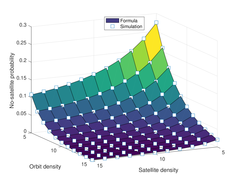
Since $r_{s},\lambda$ and $\mu$ are system parameters, large-scale impact of modifying geometry of the LEO satellite network, such as increasing the number of orbits or decreasing the satellite density, can easily be assessed. For instance, we observe that the no-satellite probability expression of Theorem 2 is exponential in the number of orbits. Fig. 4 displays the no-satellite probability when $\lambda\in(5,15)$ and $\mu\in(5,15).$ The simulation results are produced by Monte Carlo simulation with the sample size $N=10^{5}$ and the simulation results validate the accuracy of the formula derived in Theorem 2.

For the moment, suppose $\mu$ is very high. In this case, each orbit has a very large number of satellites and thus the no-satellite probability is dictated by the distribution of orbits in space. From the above formula, with $\mu\gg 1$, we have $e^{-2r_{s}\mu}\approxeq 0$ and thus the above derived no-satellite probability is asymptotically approximated as $\exp\left(-{\lambda}\sin(\overline{\varphi})\right).$ For instance, if $r_{s}=7000$ km, we have $\exp(-0.4\lambda)$. If $\lambda=52$, the no-satellite probability is approximately $10^{-9}.$

Figure 4: The no-satellite probability. The satellite altitude is $1100$ km. Simulation results validates the derived formula.

IV-B Distribution of the Distance to the Nearest Satellite

Let $D$ be the distance from the typical user to its nearest satellite. Note that when the nearest satellite is visible, we have $r_{s}-r_{e}\leq D\leq r_{s}^{2}-r_{e}^{2}$. We set $D=\infty$ if there is no visible satellite from the typical user.

Theorem 3.

$\operatorname{\mathbf{P}}(D>d)$ the CCDF of the distance to the nearest satellite is given by $1$ for $d<r_{s}-r_{e}$,

$$e^{-{\lambda}\int_{0}^{\xi(d)}\cos(\varphi)\left(1-e^{\-{\mu}{\pi}^{-1}\arcsin\left(\sqrt{1-\cos^{2}(\xi(d))\sec^{2}(\varphi)}\right)}\right)\mathop{}\!\mathrm{d}\varphi},$$

for $r_{s}-r_{e}\leq d<\sqrt{r_{s}^{2}-r_{e}^{2}}$, where $\xi(d)=\arccos\left(({r_{s}^{2}+r_{e}^{2}-d^{2}})/({2r_{e}r_{s}})\right)$, and is equal to the no-satellite probability for $d\geq\sqrt{r_{s}^{2}-r_{e}^{2}}.$

Proof:

The distance to the nearest visible satellite is greater than $d$ if and only if all the satellites are at distances greater than $d$. Since the orbit radius is $r_{s}$, the CCDF is $1$ for $d<r_{s}-r_{e}.$

For $r_{s}-r_{e}\leq d<\sqrt{r_{s}^{2}-r_{e}^{2}},$ we exploit Appendix A and the proof of Theorem 2 to obtain

$$\operatorname{\mathbf{P}}(D>d)$$

$$=e^{-{\lambda}\int_{\pi/2-\xi(d)}^{\pi/2+\xi(d)}\frac{\sin(\phi)}{2}\left(1-e^{-\frac{\mu}{\pi}\sin^{-1}\left(\sqrt{1-\cos^{2}(\xi(d))\csc^{2}(\phi)}\right)}\right)\mathop{}\!\mathrm{d}\phi}$$

$$=e^{-{\lambda}\int_{0}^{\xi}\cos(\varphi)\left(1-e^{-\frac{\mu}{\pi}\sin^{-1}\left(\sqrt{1-\cos^{2}(\xi(d))\sec^{2}(\varphi)}\right)}\right)\mathop{}\!\mathrm{d}\varphi},$$

where we use the fact that only the orbits having inclinations between $\pi/2-\xi(d)$ and $\pi/2+\xi(d)$ will meet the spherical cap $C_{d}$. For $r_{s}-r_{e}\leq d<\sqrt{r_{s}^{2}-r_{e}^{2}},$ we have

$$\xi(d)=\arccos\left(({r_{s}^{2}+r_{e}^{2}-d^{2}})/({2r_{s}r_{e}})\right).$$

Note that $d$ denotes the distance to the nearest satellite and it is the value that $D$ will take.

For $d\geq\sqrt{r_{s}^{2}-r_{e}^{2}},$ the CCDF evaluated at such $d$ is the probability that there is no visible satellite, namely the no-satellite probability of Theorem 2. ∎

V Coverage Probability

This section evaluates the coverage probability of the typical user. We start with the Rayleigh fading case.

Theorem 4.

In the interference-limited regime with $m=1$, namely in Rayleigh fading environment, the coverage probability of the typical user is given by Eq. (15).

$$\int_{r_{s}-r_{e}}^{\sqrt{r_{s}^{2}-r_{e}^{2}}}\frac{\lambda\mu z}{\pi r_{s}r_{e}}\exp\left(-{\lambda}\int_{\xi(z)}^{\bar{\varphi}}\left(1-e^{-\frac{\mu}{\pi}\int_{0}^{\omega_{2}(\nu)}\left(1-\operatorname{\mathcal{L}}_{H}(\frac{\tau z^{\alpha}}{g\overline{K_{\nu,\omega}}^{\alpha}})\right)\mathop{}\!\mathrm{d}\omega}\right)\cos(\nu)\mathop{}\!\mathrm{d}\nu\right)$$

$$\hskip 48.36967pt\times\exp\left(-{\lambda}\int_{0}^{\xi(z)}\left(1-e^{-\frac{\mu}{\pi}\arcsin(\sqrt{1-\cos^{2}(\xi(z))\sec^{2}(\nu)})-\frac{\mu}{\pi}\int_{\omega_{1}(\nu,z)}^{\omega_{2}(\nu)}\left(1-\operatorname{\mathcal{L}}_{H}(\frac{\tau z^{\alpha}}{g\overline{K_{\nu,\omega}}^{\alpha}})\right)\mathop{}\!\mathrm{d}\omega}\right)\cos(\nu)\mathop{}\!\mathrm{d}\nu\right)$$

$$\hskip 48.36967pt\times\left(\int_{0}^{{\xi(z)}}\frac{e^{-\frac{\mu}{\pi}\arcsin(\sqrt{1-\cos^{2}(\xi(z))\sec^{2}(\varphi)})-\frac{\mu}{\pi}\int_{\omega_{1}(\varphi,z)}^{\omega_{2}(\varphi)}\left(1-\operatorname{\mathcal{L}}_{H}(\frac{\tau z^{\alpha}}{g\overline{K_{\varphi,\omega}}^{\alpha}})\right)\mathop{}\!\mathrm{d}\omega}}{\sqrt{1-\cos^{2}(\xi(z))\sec^{2}(\varphi)}}\mathop{}\!\mathrm{d}\varphi\right)\mathop{}\!\mathrm{d}z.$$ (15)

 

Proof:

Let $X_{\star}$ denote the location of the satellite nearest to the typical user at $n$, $I$ the power of the interference created by the visible satellites at distances greater than $\|X_{\star}-n\|$, and $g$ the aggregate antenna gain when the transmit and receiver antennas are aligned to provide the maximum antenna gain, namely $g=g_{1}+g_{2}$. We have

$$\operatorname{\mathbf{P}}(\operatorname{\textnormal{SINR}}>\tau)= \operatorname{\mathbf{E}}\left[\operatorname{\mathcal{L}}_{I}\left(\frac{\tau\|X_{\star}-n\|^{\alpha}}{pg}\right)\right],$$ (16)

where $\operatorname{\mathcal{L}}_{I}(s)$ is the Laplace transform of $I$. We used here the fact that, for $m=1,$ $H$ follows an exponential random variable with mean one independent of $I$ and $X_{\star}$.

The difficulty with Eq. (16) is that the random variables $I$ and $\|X_{\star}-n\|$ are not independent. In order to compute their joint distribution, we proceed in 3 main steps.

The first step consists in introducing a partition of all possibilities concerning $D$ and the orbit that contains $X_{\star}$. Let $i_{\star}$ denote the index of the latter. We have

$$\operatorname{\mathbf{E}}\left[\operatorname{\mathcal{L}}_{I}\left(\frac{\tau\|X_{\star}-n\|^{\alpha}}{pg}\right)\right]$$ (17)

$$=\int\limits_{z}\operatorname{\mathbf{E}}\left[\sum_{i}\operatorname{\mathcal{L}}_{I}\left(\frac{\tau z^{\alpha}}{pg}\right)1_{i_{\star}=i}1_{D\in[z,z+dz]}\right]$$

$$\stackrel{{\scriptstyle(\text{a})}}{{=}}\int\limits_{z}\int\limits_{(\theta,\phi)}\operatorname{\mathbf{E}}^{0}_{\theta,\phi}\left[\operatorname{\mathcal{L}}_{I}\left(\frac{\tau z^{\alpha}}{pg}\right)1_{l_{i_{\star}}=l(\theta,\phi)}1_{D\in[z,z+dz]}\right]$$

$$\hskip 113.81102pt\Lambda(\mathop{}\!\mathrm{d}\theta,\mathop{}\!\mathrm{d}\phi)$$

$$\stackrel{{\scriptstyle(\text{b})}}{{=}}\lambda\int\limits_{z}\int\limits_{\phi}\operatorname{\mathbf{E}}^{0}_{\theta,\phi}\left[\operatorname{\mathcal{L}}_{I}\left(\frac{\tau z^{\alpha}}{pg}\right)1_{\phi_{i_{\star}}=\phi}1_{D\in[z,z+dz]}\right]\sin(\phi)\mathop{}\!\mathrm{d}\phi,$$

where $\operatorname{\mathbf{E}}^{0}_{\theta,\phi}$ denotes the Palm probability of $\Xi$. In (a), we used Campbell’s formula. In (b), we used that fact that the function of interest are invariant by a change of $\theta$. Note that the law of $\Xi$ under the Palm probability in question is the law of $\Xi+\delta_{(\theta,\phi)}$, with $\Xi$ distributed as above. Hence

$$\operatorname{\mathbf{E}}^{0}_{\theta,\phi}\left[\operatorname{\mathcal{L}}_{I}\left(\frac{\tau z^{\alpha}}{pg}\right)1_{\phi_{i_{\star}}=\phi}1_{D\in[z,z+dz]}\right]$$ (18)

$$= \operatorname{\mathbf{E}}\left[\operatorname{\mathcal{L}}_{\widehat{I}}\left(\frac{\tau z^{\alpha}}{pg}\right)1_{\phi_{\widehat{i}_{\star}}=\phi}1_{\widehat{D}\in[z,z+dz]}\right],$$

with $\widehat{I}$, $\widehat{i}_{\star}$ and $\widehat{D}$ for $\Xi+\delta_{(\theta,\phi)}$ in place of $\Xi$.

Let $\mathcal{F}$ be the sigma-algebra generated by $\Xi$. We have

$$\operatorname{\mathbf{E}}\left[\operatorname{\mathcal{L}}_{\widehat{I}}\left(\frac{\tau z^{\alpha}}{pg}\right)1_{\phi_{\widehat{i}_{\star}}=\phi}1_{\widehat{D}\in[z,z+dz]}\right]$$ (19)

$$= \operatorname{\mathbf{E}}\left[\operatorname{\mathbf{E}}\left[\operatorname{\mathcal{L}}_{\widehat{I}}\left(\frac{\tau z^{\alpha}}{pg}\right)1_{\phi_{\widehat{i}_{\star}}=\phi}1_{\widehat{D}\in[z,z+dz]}\mid{\mathcal{F}}\right]\right]$$

and, by first principles,

$$\operatorname{\mathbf{E}}\left[\operatorname{\mathcal{L}}_{\widehat{I}}\left(\frac{\tau z^{\alpha}}{pg}\right)1_{\phi_{\widehat{i}_{\star}}=\phi}1_{\widehat{D}\in[z,z+dz]}\mid{\mathcal{F}}\right]$$

$$= \operatorname{\mathbf{E}}\left[\operatorname{\mathcal{L}}_{\widehat{I}}\left(\frac{\tau z^{\alpha}}{pg}\right)\mid\phi_{\widehat{i}_{\star}}=\phi,\widehat{D}\in[z,z+dz],{\mathcal{F}}\right]$$

$$\hskip 56.9055pt\operatorname{\mathbf{P}}\left[\phi_{\widehat{i}_{\star}}=\phi,\widehat{D}\in[z,z+dz]\mid{\mathcal{F}}\right].$$

The next steps consist in computing the two terms in the last expression. We start with the conditional Laplace transform of the interference $\widehat{I}$. As we now show, conditionally on $\mathcal{F}$ and the event $\widehat{\mathcal{G}}(z)$ that $\phi_{\widehat{i}_{\star}}=\phi$ and $\widehat{D}\in[z,z+dz]$, the interference created by the satellites on different orbits are conditionally independent and there is a closed form for the Laplace transform of the interference on each orbit. To derive this closed form, we use

$$\xi(z) =\arccos\left({(r_{s}^{2}+r_{e}^{2}-z^{2})}/{(2r_{s}r_{e})}\right).$$ (21)

The angle $\xi(z)$ is that between the north direction and any point on the rim of the spherical cap $C_{z}$ for $r_{s}-r_{e}<z<\bar{d}=\sqrt{r_{s}^{2}-r_{e}^{2}}$. Then we need the following

$$K_{i,\omega} =\sqrt{r_{s}^{2}-2r_{s}r_{e}\sin(\omega)\sin({\phi}_{i})+r_{e}^{2}},$$ (22)

$$K_{\omega} =\sqrt{r_{s}^{2}-2r_{s}r_{e}\sin(\omega)\sin({\phi})+r_{e}^{2}},$$ (23)

$$\kappa_{i,1} ={\pi}/{2}-\arcsin(\sqrt{1-(r_{e}/r_{s})^{2}\csc^{2}(\phi_{i})}),$$ (24)

$$\kappa_{1} ={\pi}/{2}-\arcsin(\sqrt{1-(r_{e}/r_{s})^{2}\csc^{2}(\phi)}),$$ (25)

$$\kappa_{i,2}(z) ={\pi}/{2}-\arcsin(\sqrt{1-{\cos^{2}(\xi(z))}{\csc^{2}(\phi_{i})}}),$$ (26)

$$\kappa_{2}(z) ={\pi}/{2}-\arcsin(\sqrt{1-{\cos^{2}(\xi(z))}{\csc^{2}(\phi)}}).$$ (27)

The function $K_{i,\omega}$ gives the distance between the typical user and the point of orbit $l(\theta_{i},\phi_{i})$ with orbital angle $\omega$. The function $\kappa_{i,2}(z)$ gives the angle (in the orbital plane of orbit $i$, i.e., $l(\theta_{i},\phi_{i})$) between the apex of the orbit and the point of the orbit where the distance to $n$ is $z$. The parameter $\kappa_{i,1}$ is the angle (in the orbital plane of orbit $i$) between the apex of the orbit and the point of the orbit beyond which a satellite is no more visible from $n$.

Let ${\mathcal{E}}(z)={\mathcal{F}}\cap\widehat{\mathcal{G}}(z)$. For short we use the notation $\mathcal{E}$ for ${\mathcal{E}}(z)$. Let $N$ denote the number of points of $\xi$ and let $(\theta_{i},\phi_{i}),\ i=1,\ldots,N$, denote their coordinates. Let $\psi_{i}$ denote the linear Poisson point process on $l(\theta_{i},\phi_{i})$. Note that these random variables are $\mathcal{F}$-measurable. Using the conditional independence alluded to above, and the independence of the number of points of the linear Poisson point processes on disjoint subsets of an orbit, we get

$$\operatorname{\mathcal{L}}_{\widehat{I}|{\mathcal{E}}}(s)= \operatorname{\mathbf{E}}_{\psi}\left[\prod_{X_{j}\in\psi}^{\overline{d}>K_{j}>z}\operatorname{\mathcal{L}}_{H}(spK_{j}^{-\alpha})\right]$$

$$\prod_{i=1,N}^{|\phi_{i}-\pi/2|<\overline{\varphi}}\operatorname{\mathbf{E}}_{\psi_{i}}\left[\prod_{X_{j,i}\in\psi_{i}}^{\overline{d}>K_{i,j}>z}\operatorname{\mathcal{L}}_{H}(spK_{i,j}^{-\alpha})\mid\mathcal{E}\right].$$

Then, we have

$$\operatorname{\mathcal{L}}_{\widehat{I}|{\mathcal{E}}}(s) =\exp\left(-\frac{\mu}{\pi}\int_{\kappa_{1}}^{\kappa_{2}(z)}\left(1-\operatorname{\mathcal{L}}_{H}(spK_{\omega}^{-\alpha})\right)\mathop{}\!\mathrm{d}\omega\right)$$

$$\prod_{i=1,N}^{|\phi_{i}-\pi/2|\leq\xi(z)}\exp\left(-\frac{\mu}{\pi}\int_{\kappa_{i,1}}^{\kappa_{i,2}(z)}\left(1-\operatorname{\mathcal{L}}_{H}(spK_{i,\omega}^{-\alpha})\right)\mathop{}\!\mathrm{d}\omega\right)$$

$$\prod_{i=1,N}^{\xi(z)<|\phi_{i}-\pi/2|<\overline{\varphi}}\exp\left(-\frac{\mu}{\pi}\int_{\kappa_{i,1}}^{\pi/2}\left(1-\operatorname{\mathcal{L}}_{H}(spK_{i,\omega}^{-\alpha})\right)\mathop{}\!\mathrm{d}\omega\right),$$

where $\operatorname{\mathcal{L}}_{H}(s)$ denotes the Laplace transform of the mean 1 exponential random variable. Using the change of variables $\omega\to\pi/2-\omega$, we get

$$\operatorname{\mathcal{L}}_{\widehat{I}|{\mathcal{E}}}(s) =\exp\left({-\frac{\mu}{\pi}\int_{\omega_{1}(z)}^{\omega_{2}}1-\operatorname{\mathcal{L}}_{H}(sp\widetilde{K_{\omega}}^{-\alpha})}\mathop{}\!\mathrm{d}\omega\right)$$

$$\prod_{i=1,N}^{|\phi_{i}-\pi/2|<{\xi(z)}}\exp\left({-\frac{\mu}{\pi}\int_{\omega_{i,1}(z)}^{\omega_{i,2}}1-\operatorname{\mathcal{L}}_{H}(sp\widetilde{K_{i,\omega}}^{-\alpha})}\mathop{}\!\mathrm{d}\omega\right)$$

$$\prod_{i=1,N}^{\xi(z)<|\phi_{i}-\pi/2|<\overline{\varphi}}\exp\left({-\frac{\mu}{\pi}\int_{0}^{\omega_{i,2}}1-\operatorname{\mathcal{L}}_{H}(sp\widetilde{K_{i,\omega}}^{-\alpha})}\mathop{}\!\mathrm{d}\omega\right),$$ (28)

where

$$\omega_{i,1}(z) =\arcsin(\sqrt{1-{\cos^{2}(\xi(z))}{\sec^{2}(\phi_{i})}}),$$ (29)

$$\omega_{1}(z) =\arcsin(\sqrt{1-{\cos^{2}(\xi(z))}{\sec^{2}(\phi)}}),$$ (30)

$$\omega_{i,2} =\arcsin(\sqrt{1-(r_{e}/r_{s})^{2}\sec^{2}(\phi_{i})}),$$ (31)

$$\omega_{2} =\arcsin(\sqrt{1-(r_{e}/r_{s})^{2}\sec^{2}(\phi)}),$$ (32)

$$\widetilde{K_{i,\omega}} =\sqrt{r_{s}^{2}-2r_{s}r_{e}\cos(\omega)\sin({\phi}_{i})+r_{e}^{2}}.$$ (33)

Our third step consists in computing the following conditional probability

$$\operatorname{\mathbf{P}}(\widehat{\mathcal{G}}(z)\mid{\mathcal{F}})=\operatorname{\mathbf{P}}(\exists j_{\star}\in\psi:\|X_{j_{\star}}-n\|\in[z,z+\mathop{}\!\mathrm{d}z],$$

$$\hskip 8.5359pt\forall j\neq j_{\star},\|X_{j}-n\|>z,\forall i=1,N,\forall j,\|X_{i,j}-n\|>z|{\mathcal{F}}).$$

Using now the fact that the length of the arc $C_{z}\cap l(\theta_{i},\phi_{i})$ is $2r_{s}\arcsin\left(\sqrt{1-\cos^{2}(\xi(z))\csc^{2}(\phi_{i})}\right)$, we get

$$\operatorname{\mathbf{P}}(\widehat{D}\in[z,z+\mathrm{d}z),\phi_{\widehat{i_{\star}}}=\phi\mid{\mathcal{F}})$$ (34)

$$=\frac{\partial}{\partial z}\left(1-e^{-\frac{\mu}{\pi}\arcsin\left(\sqrt{1-\cos^{2}(\xi(z))\csc^{2}(\phi)}\right)}\right)\mathop{}\!\mathrm{d}z$$

$$\hskip 17.07164pt\prod^{\pi/2-\xi(z)<\phi_{i}<\pi/2+\xi(z)}_{i=1,N}e^{-\frac{\mu}{\pi}\arcsin\left(\sqrt{1-\cos^{2}(\xi(z))\csc^{2}(\phi_{i})}\right)}$$

$$=\frac{\mu z|\csc(\phi)|e^{-\frac{\mu}{\pi}\arcsin\left(\sqrt{1-\cos^{2}(\xi(z))\csc^{2}(\phi)}\right)}}{\pi r_{e}r_{s}\sqrt{1-\cos^{2}(\xi(z))\csc^{2}(\phi)}}$$

$$\hskip 17.07164pt\prod^{\pi/2-\xi(z)<\phi_{i}<\pi/2+\xi(z)}_{i=1,N}e^{-\frac{\mu}{\pi}\arcsin\left(\sqrt{1-\cos^{2}(\xi(z))\csc^{2}(\phi_{i})}\right)},$$

where $\cos(\xi(z))$ is given by Eq. (21). Here, we used the fact that conditionally on $\mathcal{F}$, the satellite point processes on orbits are independent Poisson point processes.

We now plug in Eq. (28) and (34) (together with (18), (19), and (V)) in (17) to get (15). This expression is obtained by using the Laplace functional of the Poisson point process $\Xi$ and by the change of variable $\varphi=\pi/2-\phi$. It uses the functions

$$\overline{K_{\varphi,\omega}} =\sqrt{r_{s}^{2}-2r_{s}r_{e}\cos(\omega)\cos(\varphi)+r_{e}^{2}},$$

$$\omega_{1}(\varphi,z) =\arcsin(\sqrt{1-{\cos^{2}(\xi(z))}{\sec^{2}(\varphi)}}),$$

$$\omega_{2}(\varphi) =\arcsin(\sqrt{1-(r_{e}/r_{s})^{2}\sec^{2}(\varphi)}).$$

This completes the proof. ∎

In a case that thermal noise cannot be neglected, the coverage probability of the typical user can be assessed by scaling the formula in Theorem 5 with a constant.

Theorem 5 gives the coverage probability of the typical user in terms of $\lambda$ the mean number of orbits, $\mu$ the mean number of satellites per orbit, $r_{s}$ radius of orbit, and $g$ the aggregate antenna gain. As our Cox-distributed satellite model exhibits rotation invariance, the coverage probability of the typical user at $n$ statistically coincides with the coverage probabilities of all users in the network. Consequently, the derived coverage probability captures the fundamental performance of the LEO satellite network. By utilizing this formula, one can readily forecast and estimate the behavior of the coverage probability with varying the aforementioned geometric parameters.

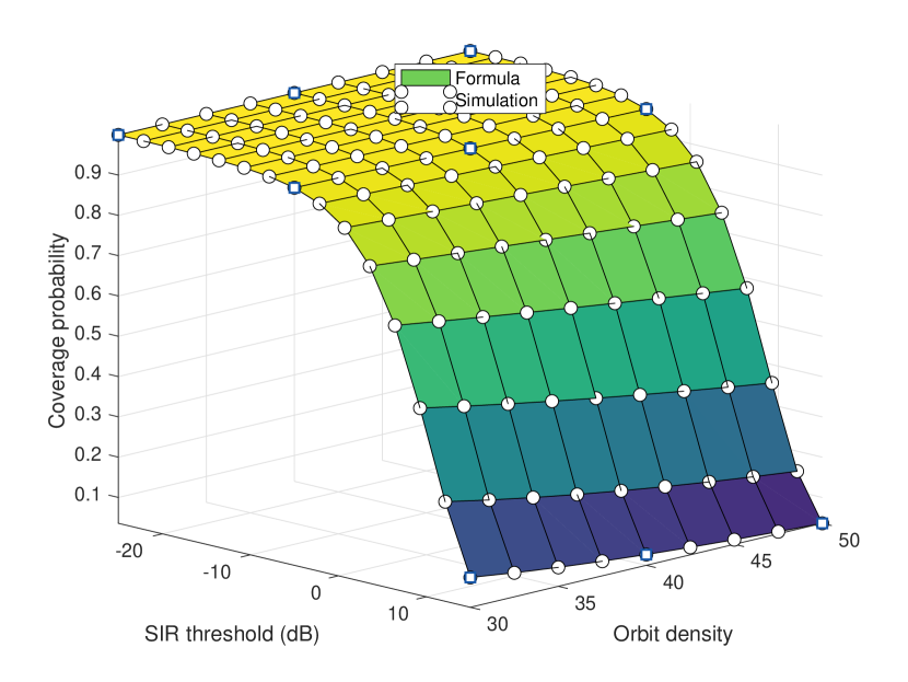
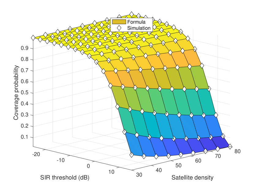
Fig. 5 and 6 illustrate the coverage probability of the typical user for various values of $\lambda$ and $\mu$. The simulation results validate the accuracy of the derived formula in Theorem 5. While obtaining simulation results necessitates significant computation time due to the construction of large-scale network layout, the derived formula enables the generation of the entire coverage probability graph in much less time. This efficiency facilitates the execution of complex multivariate analyses of LEO satellite networks, that we will see shortly. In the following, we explore the coverage behavior of the LEO satellite network by varying various geometric parameters.

Figure 5: The coverage probability of the network with $\mu=30$, $r=7050$ km, and $g=20$ dB. Simulation results validate the derived formula.

Figure 6: The coverage probability of the network with $\lambda=30$, $r=6950$ km, and $g=20$ dB.

Figure 7: The coverage probability of the network with $\lambda=30$, $\mu=30$, and $g=20$ dB. The formula is validated through simulation results.

Figure 8: The $0$-dB coverage probability of the network with $r_{s}=6950$ km and $g=20$ dB.

Figure 9: The $0$-dB coverage probability of the network with $\lambda=30$ and $r_{s}=6950$ km

Figure 10: The $0$-dB coverage probability of the network with $\lambda=30$ and $\mu=40$.

$$\int_{0}^{\infty}\int_{r_{s}-r_{e}}^{\sqrt{r_{s}^{2}-r_{e}^{2}}}\frac{\lambda\mu z}{\pi r_{s}r_{e}}\exp\left(-{\lambda}\int_{\xi(z)}^{\bar{\varphi}}\left(1-e^{-\frac{\mu}{\pi}\int_{0}^{\omega_{2}({\varphi})}\left(1-\operatorname{\mathcal{L}}_{H}((2^{u}-1)z^{\alpha}/(g\overline{K_{\varphi,\omega}}^{\alpha}))\right)\mathop{}\!\mathrm{d}\omega}\right)\cos(\varphi)\mathop{}\!\mathrm{d}\varphi\right)$$

$$\hskip 56.9055pt\times\exp\left(-{\lambda}\int_{0}^{\xi(z)}\left(1-e^{-\frac{\mu}{\pi}\arcsin(\sqrt{1-\cos(\xi(z))^{2}\sec(\varphi)^{2}})-\frac{\mu}{\pi}\int_{\omega_{1}{(\varphi,z)}}^{\omega_{2}{(\varphi)}}\left(1-\operatorname{\mathcal{L}}_{H}((2^{u}-1)z^{\alpha}/(g\overline{K_{\varphi,\omega}}^{\alpha}))\right)\mathop{}\!\mathrm{d}\omega}\right)\cos(\varphi)\mathop{}\!\mathrm{d}\varphi\right)$$

$$\hskip 56.9055pt\times\left(\int_{0}^{{\xi(z)}}\frac{e^{-\frac{\mu}{\pi}\arcsin(\sqrt{1-\cos(\xi(z))^{2}\sec(v)^{2}})-\frac{\mu}{\pi}\int_{\omega_{1}{(v,z)}}^{\omega_{2}{(v)}}\left(1-\operatorname{\mathcal{L}}_{H}((2^{u}-1)z^{\alpha}/(g\overline{K_{v,\omega}}^{\alpha}))\right)\mathop{}\!\mathrm{d}\omega}}{\sqrt{1-\cos^{2}(\xi(z))\sec^{2}(v)}}\mathop{}\!\mathrm{d}v\right)\mathop{}\!\mathrm{d}z\mathop{}\!\mathrm{d}u.$$ (35)

 

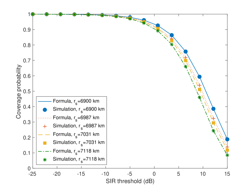
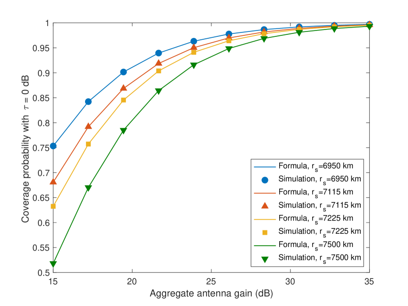
Fig. 7 displays the impact of satellite altitude on coverage probability. For the given $\lambda$ and $\mu$, it is observed that higher satellite altitudes typically lead to lower coverage probabilities. It is worth noting that the difference in coverage probability from various satellite altitudes is noticeable for higher thresholds.

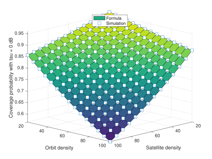
Fig. 8 shows the $0$-dB coverage probability, namely the probability that the typical user has the SINR is greater than $0$ dB. The $0$-dB coverage probability of the typical user also indicates the total fraction of network users having their SINR greater than $0$ dB. Such an interpretation leads to important insights for LEO satellite network design or optimization. For instance, for $\lambda=50$ and $\mu=50$, about 85% of users have SINR greater than $0$ dB. For $\lambda=100$ and $\mu=50$ or $\lambda=50$ and $\mu=100$, where the total average numbers of LEO satellites are the same, their $0$-dB coverage probabilities are almost identical, at $0.74$. A deployment plan of forthcoming LEO satellite constellation—such as adding orbits or adding satellites on each orbit—can be effectively evaluated by adapting the proposed framework, offering a comprehensive tool to design LEO satellite networks for network operators.

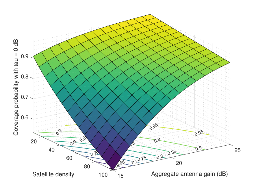
Fig. 9 gives the $0$-dB coverage probability for various $\mu$ and $g$. In practice, LEO satellite network operators deploy more satellites to cope with an increased number of ground users. Yet, this may lead to increased interference or decreased coverage due to the additional satellites. Occupying additional orbital planes may not be a feasible option, and in this case, a viable solution may be to deploy new LEO satellites with better antenna gain. Using the derived formula, Fig. 9 shows how much antenna gain from the LEO satellite is required to attain the same coverage probability level for various densities of $\mu$. For instance, if the satellite density $\mu$ changes from $\mu_{1}$ to $\mu_{2}$, the network operator may also need additional antenna gain from $g_{1}$ to $g_{2}$ to ensure the same quality of service for network users. In the same vein, we conduct a similar experiment in Fig. 10 where we examine the coverage benefit of having additional antenna gain for satellite altitudes.

Corollary 1.

The achievable rate or the ergodic capacity of downlink LEO satellite communications is given by Eq. (35).

Proof:

The achievable rate or the ergodic capacity is

Throughput $$=\int_{0}^{\infty}\operatorname{\mathbf{P}}(\log_{2}(1+\operatorname{\textnormal{SINR}})>r)\mathop{}\!\mathrm{d}r$$

$$=\int_{0}^{\infty}\operatorname{\mathbf{P}}(\operatorname{\textnormal{SINR}}>2^{r}-1)\mathop{}\!\mathrm{d}r,$$ (36)

where we use the fact that $\log_{2}(1+\operatorname{\textnormal{SINR}})$ is a positive random variable. ∎

$$\sum_{k=0}^{m-1}\frac{\lambda}{2k!}\int\limits_{r_{s}-r_{e}}^{\sqrt{r_{s}^{2}-r_{e}^{2}}}\int\limits_{\pi/2-\xi}^{\pi/2+\xi}\!\operatorname{\mathbf{E}}_{{\Xi}}\!\!\left[\left\{(-s)^{k}\frac{\partial^{k}}{\partial s^{k}}\left(h_{1}(z,v,s)\prod^{0<|\phi_{i}-\pi/2|<\xi}_{(\theta_{i},\phi_{i})\in\Xi}h_{1}(z,\phi_{i},s)\prod^{\xi<|\phi_{i}-\pi/2|<\overline{\varphi}}_{(\theta_{i},\phi_{i})\in\Xi}h_{2}(z,\phi_{i},s)\right)\right\}_{s=\frac{m\tau z^{\alpha}}{pg}}\right.$$

$$\hskip 136.57323pt\left.\frac{\mu ug(z,v)\prod\limits_{(\theta_{i},\phi_{i})\in\Xi}^{|\phi_{i}-\pi/2|<\xi}g(z,\phi_{i})}{\pi r_{e}r_{s}\sqrt{1-{\cos^{2}(\xi)}{\csc^{2}(v)}}}\right]\mathop{}\!\mathrm{d}v\mathop{}\!\mathrm{d}z.$$ (37)

 

In below, we derive the coverage probability of the typical user for a general fading with $m=1,2,...$

Theorem 5.

In the interference-limited regime with general $m,$ the coverage probability of the typical user is given by Eq. (37) where $\xi,$ $\omega_{i,1}(z)$, $\omega_{i,2}$, $\widetilde{K_{i,\omega}}$ are given by Eqs. (21), (29), (31), and (33), respectively. We also have

$$h_{1}(z,\phi_{i},s) {=}\exp\left({-\frac{\mu}{\pi}\int_{\omega_{i,1}(z)}^{\omega_{i,2}}1-\operatorname{\mathcal{L}}_{H}(sp/\widetilde{K_{i,\omega}}^{\alpha})}\mathop{}\!\mathrm{d}\omega\right),$$

$$h_{2}(z,\phi_{i},s) {=}\exp\left({-\frac{\mu}{\pi}\int_{0}^{\omega_{i,2}}1-\operatorname{\mathcal{L}}_{H}(sp/\widetilde{K_{i,\omega}}^{\alpha})}\mathop{}\!\mathrm{d}\omega\right),$$

$$g(z,\phi) {=}\exp\left({-\frac{\mu}{\pi}\arcsin\left(\sqrt{1-\cos^{2}(\xi(z))\csc^{2}(\phi)}\right)}\right).$$

Proof:

As in the proof of Theorem 4, in the interference-limited regime, the coverage probability of the network is

$$\operatorname{\mathbf{P}}(\operatorname{\textnormal{SINR}}>\tau)$$

$$=\operatorname{\mathbf{E}}_{\Xi}\left[\operatorname{\mathbf{P}}\left(\left.H>\frac{\tau I\|X_{\star}-n\|^{\alpha}}{pg}\right|\Xi\right)\right]$$

$$=\operatorname{\mathbf{E}}_{\Xi,l_{\star},D,I}\left.\left.\left.\left[\left.e^{-\frac{m\tau Iz^{\alpha}}{pg}}\sum_{k=0}^{m-1}\frac{\frac{m^{k}\tau^{k}I^{k}z^{k\alpha}}{p^{k}g^{k}}}{k!}\right|D,l_{\star}\Xi\right.\right]\right]\right]$$

$$=\sum_{k=0}^{m-1}\frac{1}{k!}\operatorname{\mathbf{E}}_{\Xi,l_{\star},D}\left.\!\left.\left[\left.s^{k}(-1)^{k}\frac{\partial^{k}}{\partial s^{k}}\operatorname{\mathcal{L}}_{I|D,l_{\star},\Xi}(s)\right|_{s=\frac{m\tau z^{\alpha}}{pg}}\right.\right.\right],$$

where we used the probability distribution function of the Nakagami-$m$ random variable. We also used the fact that the $k$-th moment of the interference can be obtained by taking the $k$-order derivative of the Laplace transform of the interference. Hence, we have

$$\operatorname{\mathbf{E}}_{I}\!\!\left[\left.e^{-\frac{m\tau Iz^{\alpha}}{pg}}\sum_{k=0}^{m-1}\frac{\frac{m^{k}\tau^{k}I^{k}z^{k\alpha}}{p^{k}g^{k}}}{k!}\right|\operatorname{\mathcal{E}}\right]\!\! =\!\!\left.\sum_{k=0}^{m-1}\frac{(-s)^{k}}{k!}\frac{\partial^{k}}{\partial s^{k}}\operatorname{\mathcal{L}}_{I|\operatorname{\mathcal{E}}}(s)\right.,$$

where ${s=\frac{m\tau z^{\alpha}}{pg}}$. As in the proof of Theorem 4, we have

$$\operatorname{\mathcal{L}}_{I|\operatorname{\mathcal{E}}}(s) =\exp\left({-\frac{\mu}{\pi}\int_{\omega_{1}(z)}^{\omega_{2}}1-\operatorname{\mathcal{L}}_{H}(sp\widetilde{K_{\omega}}^{-\alpha})}\mathop{}\!\mathrm{d}\omega\right)$$

$$\prod_{i=1,N}^{|\phi_{i}-\pi/2|<{\xi(z)}}\exp\left({-\frac{\mu}{\pi}\int_{\omega_{i,1}(z)}^{\omega_{i,2}}1-\operatorname{\mathcal{L}}_{H}(sp/\widetilde{K_{i,\omega}}^{\alpha})}\mathop{}\!\mathrm{d}\omega\right)$$

$$\prod_{i=1,N}^{\xi(z)<|\phi_{i}-\pi/2|<\overline{\varphi}}\exp\left({-\frac{\mu}{\pi}\int_{0}^{\omega_{i,2}}1-\operatorname{\mathcal{L}}_{H}(sp/\widetilde{K_{i,\omega}}^{\alpha})}\mathop{}\!\mathrm{d}\omega\right),$$ (38)

where $\operatorname{\mathcal{L}}_{H}(s)$ is the Laplace transform of the random variable $H.$ The variables $\xi$, $\omega_{i,1}(z)$, $\omega_{i,2}$, and $\widetilde{K_{i,\omega}}$ are given by Eqs. (21), (29), (31), and (33).

Conditionally on $\Xi$ and $l_{\star},$ the PDF of $D$ is given by taking the derivative of the CDF of $D$ as follows:

$$f_{D}(z)= \frac{\mu z|\csc(\phi)|e^{-\frac{\mu}{\pi}\arcsin\left(\sqrt{1-\cos^{2}(\xi(z))\csc^{2}(\phi)}\right)}}{\pi r_{e}r_{s}\sqrt{1-{\cos^{2}(\xi(z))}{\csc^{2}(\phi)}}}$$

$$\prod\limits^{|\phi_{i}-\pi/2|<\xi(z)}_{i=1,N}\!\!\!\!e^{-\frac{\mu}{\pi}\arcsin\left(\sqrt{1-\cos^{2}(\xi(z))\csc^{2}(\phi_{i})}\right)}.$$ (39)

Finally, we obtain the final result by combining all the expressions and following the same steps as in the proof of Theorem 4. ∎

VI Discussion

VI-A Cox Model to Forthcoming Constellation

In this section, we focus on describing the second-generation (2A) Starlink constellation and its satellites using the proposed Cox point process. Since the local distribution of the Starlink constellation varies with user latitudes, while the developed Cox point process is isotropic, we employ a moment-matching local approximation technique. Specifically, we adjust the orbital density and satellite density, denoted as $\lambda$ and $\mu$ in the Cox point process, to ensure that the Cox constellation and the Starlink constellation have, on average, the same number of LEO satellites.

For the upcoming Starlink constellation, we refer to the Starlink deployment plan available at the FCC [6], which involves $28$ orbital planes at an altitude of $525$ km and an inclination of $43$ degrees, $28$ orbital planes at $530$ km with an inclination of $53$ degrees, and $28$ planes at an altitude of $535$ km with an inclination of $33$ degrees. Each plane will accommodate $120$ satellites. To numerically derive the network performance of Starlink, we consider a frequency reuse factor of $4$ for the Starlink constellation, where $30$ satellites on each orbit use the same spectrum resource.

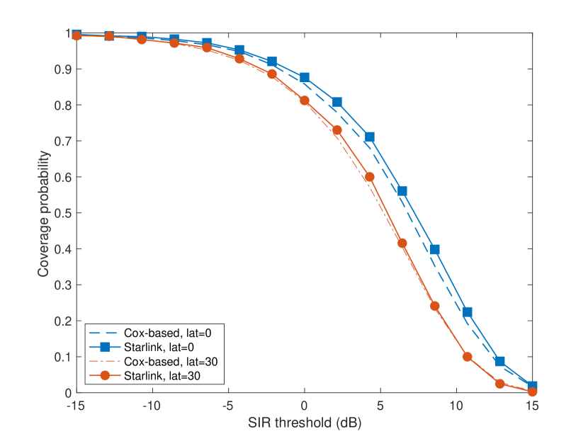
Fig. 11 illustrates the coverage probability based on the upcoming Starlink constellation and the proposed Cox point process. At a latitude of $30$ degrees, the proposed Cox point process accurately emulates the Starlink constellation. At a latitude of $0$ degree, the proposed Cox point process replicates a coverage probability comparable to that of the Starlink constellation, with differences of less than $0.5$ dB. The marginal difference arises from the geometric distinction that while the proposed Cox point process is isotropic the satellites of the forthcoming Starlink constellation are regularly separated on each orbit and the orbits’ inclinations are having only three values at $43,53,33$ degrees.

Figure 11: The coverage probability of Starlink and Cox constellations for users at latitudes of $0$ and $30$ degrees. $r_{s}=7000$ and $g=20$ dB.

VI-B Cox model and Binomial Model

This subsection highlights the advantages of our Cox point process over the binomial point process.

Analytical stochastic geometry models, such as binomial model or our Cox model, can represent existing or forthcoming target constellation through a moment matching approximation. For example, the binomial point process features a network geometric parameter, denoted as $N$, representing the number of satellites. This parameter $N$ is then fine-tuned to match the mean number of visible satellites of the target constellation. In contrast, the proposed Cox point process features two geometric parameters, $\lambda$ and $\mu$, and these two parameters are adjusted jointly to match the mean number of orbits and the mean number of satellites at the same time. Consequently, the presence of two parameters allows us to approximate the higher-order geometric characteristics of the target constellation, offering a better a representation of reality.

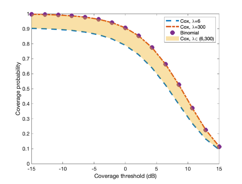
In Fig. 12, the coverage probabilities of both the binomial and Cox satellite point processes are illustrated. We consider a single target constellation having $300$ satellites at an altitude of $550$ km. The modeling technique based on the binomial point process results in a single curve for the coverage probability of the typical user. However, in the case of a modeling based on our Cox point process, its flexibility allows for a wide range of achievable coverage probabilities by varying $\lambda$ and/or $\mu$. Due to this flexibility, we observe that the coverage probability derived under the Cox point process encompasses and extends the coverage probability based on the binomial point process.

Figure 12: Our Cox model features a wide range of coverage probabilities whereas a single coverage probability curve appears for the binomial model.

VII Conclusion

We have constructed an analytical framework for modeling and analyzing downlink LEO satellite communications. By developing an isotropic Cox point process for LEO satellites, we introduced a novel method for incorporating the essential geometry of LEO satellite constellations, where satellites exclusively orbit the Earth. We calculate the no-satellite probability for the typical user. Assuming that network users receive their downlink signals from their closest satellites, we evaluate the Laplace transform of the interference and assess the coverage probability for the typical user. The derived metrics represent network performance as functions of key network parameters. Thanks to isotropy, our analysis of the typical user’s network performance can be interpreted as the network performance spatially averaged over all users across the network. Therefore, our analysis can be applied to the systematic design of large-scale downlink LEO satellite communication networks. We demonstrate that our Cox point process effectively replicates a forthcoming LEO satellite constellation through moment matching approximation. Additionally, our Cox model provides numerous ways to model real or forthcoming constellations, in contrast to models based on binomial or Poisson point processes.

Future work will concentrate on addressing the limitations of the proposed model. For example, our framework currently assumes isotropic orbits, and a similar approach can be used to explore and investigate non-isotropic orbits. Similarly, the developed isotropic orbit may feature regularly-spaced LEO satellites conditionally on each orbit. Moreover, the proposed model assumes a fixed altitude for LEO satellite networks. A similar approach can also be used to analyze LEO satellite networks at various altitudes.

Appendix A

Figure 13: Illustration of spherical caps $C_{d}$ and $C_{\overline{d}}$ where $r_{s}-r_{e}<d<\overline{d}$ where $\overline{d}$.

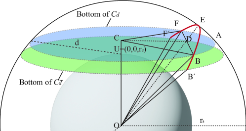
Let us treat $d$ as a constant between $r_{s}-r_{e}$ and $\sqrt{r_{s}^{2}-r_{e}^{2}}$ for the moment. Fig. 13 shows the bottom of spherical cap $C_{d}$ where the arc ¿ $\textstyle BF$ is defined as $C_{d}\cap l(\theta,\varphi)$.

For a triangle $\triangle AOU,$ in Fig. 13 $\overline{AO}=r_{s}$ and let $\xi$ be the angle $\angle AOU$. Then, we have $\cos(\xi)=\frac{r_{s}^{2}+r_{e}^{2}-d^{2}}{2r_{e}r_{s}}.$

For $\triangle BOC,$ $\angle BOC=\xi$ and we have $\overline{OB}=r_{s},\overline{OC}=r_{s}\cos(\xi),\overline{BC}=r_{s}\sin(\xi)$. Then, since the orbital plane of $l(\theta,\phi)$ has the inclination of $\phi$, $\angle DOC=\pi/2-\phi$, $\overline{OC}=r_{s}\cos(\xi),$ and $\overline{CD}=r_{s}\cos(\xi)\cot(\phi).$

For $\triangle BCD,$ we have $\overline{BC}=r_{s}\sin(\xi)$ and $\overline{CD}=r_{s}\cos(\xi)\cot(\phi)$. Since $\angle BDC=\pi/2,$ we have $\overline{BD}=\sqrt{r_{s}^{2}\sin^{2}(\xi)-r_{s}^{2}\cos^{2}(\xi)\cot^{2}(\phi)}.$

Now consider a trangle $\triangle OBD$ in the orbital plane. We have $\overline{OB}=r_{s}$ and $\overline{BD}=\sqrt{r_{s}^{2}\sin^{2}(\xi)-r_{s}^{2}\cos^{2}(\xi)\cot^{2}(\phi)}.$ Let ${\kappa}^{\prime}=\angle BOD$. Since $\angle BDO=\pi/2$, we get

$$\sin(\kappa^{\prime})=\frac{\overline{BD}}{r_{s}}=\sqrt{\sin^{2}(\xi)-\cos^{2}(\xi)\cot^{2}(\phi)}.$$ (40)

As a result, for $\pi/2-\xi<\phi<\pi/2+\xi$ the length of the arc ¿ $\textstyle BF$ is $2r_{s}\arcsin(\sqrt{1-\cos^{2}(\xi)\csc^{2}(\phi)}).$

Appendix B

Based on the simple geometry, the $(x,y,z)$ coordinates of the satellite with orbital angle $\omega_{j}$ on the orbit $l(\theta_{i},\phi_{i})$ are

$$x =\sqrt{r_{s}^{2}\cos^{2}(\omega_{j})+r_{s}^{2}\sin^{2}(\omega_{j})\cos^{2}(\phi_{i})}\cos\left(\tilde{\theta_{i}}+\theta\right),$$

$$y =\sqrt{r_{s}^{2}\cos^{2}(\omega_{j})+r_{s}^{2}\sin^{2}(\omega_{j})\cos^{2}(\phi_{i})}\sin\left(\tilde{\theta_{i}}+\theta\right),$$

$$z =r_{s}\sin(\omega_{j})\sin(\phi_{i}),$$

$$\tilde{\theta} =\arctan\left({\tan(\omega_{j})\cos(\phi_{i})}\right).$$

Moreover, the distance from $X_{j,i}$ and $n$ is given by

$$\|X_{j,i}-n\|\!=\sqrt{r_{s}^{2}-2r_{s}r_{e}\sin(\omega_{j})\sin({\phi}_{i})+r_{e}^{2}}=K_{i,j}.$$ (41)

References

- [1] Z. Qu, G. Zhang, H. Cao, and J. Xie, “LEO satellite constellation for Internet of Things,” IEEE Access, vol. 5, pp. 18 391–18 401, 2017.
- [2] Y. Su, Y. Liu, Y. Zhou, J. Yuan, H. Cao, and J. Shi, “Broadband LEO satellite communications: Architectures and key technologies,” IEEE Wireless Commn., vol. 26, no. 2, pp. 55–61, 2019.
- [3] Iridium Communications, Inc, “History of Iridium,” . [Online]. Available: https://www.iridiummuseum.com/timeline/
- [4] A. Guidotti, A. Vanelli-Coralli, M. Conti, S. Andrenacci, S. Chatzinotas, N. Maturo, B. Evans, A. Awoseyila, A. Ugolini, T. Foggi, L. Gaudio, N. Alagha, and S. Cioni, “Architectures and key technical challenges for 5G systems incorporating satellites,” IEEE Trans. Veh. Technol., vol. 68, no. 3, pp. 2624–2639, 2019.
- [5] S. Liu, Z. Gao, Y. Wu, D. W. Kwan Ng, X. Gao, K.-K. Wong, S. Chatzinotas, and B. Ottersten, “LEO satellite constellations for 5G and beyond: How will they reshape vertical domains?” IEEE Commun. Mag., vol. 59, no. 7, pp. 30–36, 2021.
- [6] Federal Communications Commission, “Kuiper systems, LLC application for authority to deploy and operate a Ka-band non-geostationary satellite orbit system,” no. SAT-LOA-20190704-00057, Jul 30 2020. [Online]. Available: https://www.fcc.gov/document/fcc-authorizes-kuiper-satellite-constellation
- [7] ——, “FCC authorizes Boeing broadband satellite constellation,” Nov. 3 2021. [Online]. Available: https://www.fcc.gov/document/fcc-authorizes-boeing-broadband-satellite-constellation
- [8] J. Fomon. Starlink slowed in Q2, competitors mounting challenges. [Online]. Available: https://www.ookla.com/articles/starlink-hughesnet-viasat-performance-q2-2022
- [9] N. Okati, T. Riihonen, D. Korpi, I. Angervuori, and R. Wichman, “Downlink coverage and rate analysis of low earth orbit satellite constellations using stochastic geometry,” IEEE Trans. Commun., vol. 68, no. 8, pp. 5120–5134, 2020.
- [10] A. Talgat, M. A. Kishk, and M.-S. Alouini, “Nearest neighbor and contact distance distribution for binomial point process on spherical surfaces,” IEEE Commun. Lett., vol. 24, no. 12, pp. 2659–2663, 2020.
- [11] ——, “Stochastic geometry-based analysis of LEO satellite communication systems,” IEEE Commun. Lett., vol. 25, no. 8, pp. 2458–2462, 2021.
- [12] D.-H. Na, K.-H. Park, Y.-C. Ko, and M.-S. Alouini, “Performance analysis of satellite communication systems with randomly located ground users,” IEEE Trans. Wireless Commun., vol. 21, no. 1, pp. 621–634, 2022.
- [13] D.-H. Jung, J.-G. Ryu, W.-J. Byun, and J. Choi, “Performance analysis of satellite communication system under the shadowed-rician fading: A stochastic geometry approach,” IEEE Trans. Commun., vol. 70, no. 4, pp. 2707–2721, 2022.
- [14] J. Park, J. Choi, and N. Lee, “A tractable approach to coverage analysis in downlink satellite networks,” IEEE Trans. Wireless Commun., vol. 22, no. 2, pp. 793–807, 2023.
- [15] S. N. Chiu, D. Stoyan, W. S. Kendall, and J. Mecke, Stochastic geometry and its applications. John Wiley & Sons, 2013.
- [16] F. Baccelli and B. Błaszczyszyn, “Stochastic geometry and wireless networks: volume I theory,” Foundations and Trends in Networking, vol. 3, no. 3–4, pp. 249–449, 2010.
- [17] ——, “Stochastic geometry and wireless networks: Volume II applications,” Foundations and Trends in Networking, vol. 4, no. 1–2, pp. 1–312, 2010.
- [18] J. G. Andrews, F. Baccelli, and R. K. Ganti, “A tractable approach to coverage and rate in cellular networks,” IEEE Trans. Commun., vol. 59, no. 11, pp. 3122–3134, 2011.
- [19] M. Haenggi, Stochastic geometry for wireless networks. Cambridge University Press, 2012.
- [20] C.-S. Choi and F. Baccelli, “Poisson Cox point processes for vehicular networks,” IEEE Trans. Veh. Technol., vol. 67, no. 10, pp. 10 160–10 165, Oct 2018.
- [21] C.-S. Choi, F. Baccelli, and G. de Veciana, “Densification leveraging mobility: An IoT architecture based on mesh networking and vehicles,” in Proc. IEEE/ACM MobiHoc, 2018, p. 71–80.
- [22] R. Wang, M. A. Kishk, and M.-S. Alouini, “Evaluating the accuracy of stochastic geometry based models for LEO satellite networks analysis,” IEEE Commun. Lett., vol. 26, no. 10, pp. 2440–2444, 2022.
- [23] V. V. Chetlur and H. S. Dhillon, “Coverage analysis of a vehicular network modeled as Cox process driven by Poisson line process,” IEEE Trans. Wireless Commun., vol. 17, no. 7, pp. 4401–4416, July 2018.
- [24] C.-S. Choi and F. Baccelli, “An analytical framework for coverage in cellular networks leveraging vehicles,” IEEE Trans. Commun., vol. 66, no. 10, pp. 4950–4964, Oct 2018.
- [25] 3GPP TR 38.821, “Solutions for NR to support non-terrestrial networks (NTN),” 3GPP TR 38.821.
- [26] M. Arti, “Two-way satellite relaying with estimated channel gains,” IEEE Trans. Commun., vol. 64, no. 7, pp. 2808–2820, 2016.
- [27] G. Zheng, S. Chatzinotas, and B. Ottersten, “Generic optimization of linear precoding in multibeam satellite systems,” IEEE Trans. Wireless Commun., vol. 11, no. 6, pp. 2308–2320, 2012.
- [28] B. Pavan Kumar, C. Kumar, V. Senthil Kumar, and V. V. Srinivasan, “Active spherical phased array design for satellite payload data transmission,” IEEE Trans. Antennas and Propagation, vol. 63, no. 11, pp. 4783–4791, 2015.
- [29] J. Zhang, M. Lin, J. Ouyang, W.-P. Zhu, and T. De Cola, “Robust beamforming for enhancing security in multibeam satellite systems,” IEEE Commun. Lett., vol. 25, no. 7, pp. 2161–2165, 2021.
- [30] M. E. Muller, “A note on a method for generating points uniformly on n-dimensional spheres,” Commun. of the ACM, vol. 2, no. 4, pp. 19–20, 1959.