Riemannian Smoothing Gradient Type Algorithms for Nonsmooth Optimization Problem on Compact Riemannian Submanifold Embedded in Euclidean Space

Abstract

In this paper, we introduce the notion of generalized $\epsilon$-stationarity for a class of nonconvex and nonsmooth composite minimization problems on compact Riemannian submanifold embedded in Euclidean space. To find a generalized $\epsilon$-stationarity point, we develop a family of Riemannian gradient-type methods based on the Moreau envelope technique with a decreasing sequence of smoothing parameters, namely Riemannian smoothing gradient and Riemannian smoothing stochastic gradient methods. We prove that the Riemannian smoothing gradient method has the iteration complexity of $\mathcal{O}(\epsilon^{-3})$ for driving a generalized $\epsilon$-stationary point. To our knowledge, this is the best-known iteration complexity result for the nonconvex and nonsmooth composite problem on manifolds. For the Riemannian smoothing stochastic gradient method, one can achieve the iteration complexity of $\mathcal{O}(\epsilon^{-5})$ for driving a generalized $\epsilon$-stationary point. Numerical experiments are conducted to validate the superiority of our algorithms.

MSC Classification]90C26, 90C30, 90C15, 90C06, 90C90

1 Introduction

We consider a general nonsmooth optimization problem on manifolds:

$$\min_{x\in\mathcal{M}}\quad\varphi(x):=f(x)+h(\mathcal{A}x),$$ (1.1)

where $\mathcal{M}$ is a compact Riemannian manifold embedded in $\mathbb{R}^{n}$, $f:\mathcal{M}\rightarrow\mathbb{R}$ is a continuously-differentiable nonconvex function; $h:\mathbb{R}^{m}\rightarrow\mathbb{R}$ is a nonsmooth weakly-convex function with a readily available proximal operator, and $\mathcal{A}:\mathbb{R}^{n}\rightarrow\mathbb{R}^{m}$ is a linear operator. The model (1.1) includes a wide range of fundamental problems such as sparse principal component analysis (SPCA) jolliffe2003modified , range-based independent component analysis selvan2013spherical ; selvan2015range , distributed optimization deng2023decentralized and robust low-rank matrix completion cambier2016robust ; hosseini2017riemannian , see Absil et al. absil2017collection for more examples. In those applications, $h$ is often a sparse regularization function, and problem (1.1) becomes a sparse optimization problem on Riemannian manifolds.

In many applications of model (1.1), $\mathcal{M}$ is a submanifold embedded in Euclidean space, for example, Stiefel manifold. There has a connection in function properties over Riemannian manifolds and Euclidean space, including smoothness and convexity. So it allows us to extend some classical optimization methods in Euclidean space to Riemannian manifolds. Indeed, many classical optimization methods for smooth optimization problems in Euclidean space have been successfully generalized to the problems on Riemannian manifolds, e.g., gradient-based methods Luenberger1972The ; grocf , Newton-based methods Absil2007Trust ; HuaAbsGal2018 ; hu2018adaptive , splitting based methods Kovna2015 ; deng2022manifold and stochastic gradient methods bonnabel2013stochastic ; sato2019riemannian ; shah2021stochastic . The reader is referred to boumal2023intromanifolds ; sato2021riemannian ; hu2020brief for a comprehensive review. However, these methods are not adapted to problem (1.1) since there exists a nonsmooth term in the objective. In this paper, we propose a homotopy smoothing method to solve problem (1.1) in some general settings. Firstly, we utilize the Moreau envelope technique to obtain a smooth approximation of nonsmooth function $h$ and employ Riemannian optimization methods to the resulted smoothing problem. Then, we apply a homotopy technique during the iterations to obtain a good enough approximation by gradually decreasing the homotopy parameter. By combining Riemannian optimization methods, smoothing techniques, and several additional assumptions, the proposed method can achieve better convergence results (computational complexity) than the existing subgradient methods.

1.1 Related works

1.1.1 Lipschitz continuous function minimization

Riemannian gradient sampling methods are motivated by gradient sampling algorithms for nonconvex nonsmooth optimization in Euclidean space. As introduced in hosseini2018line ; hosseini2017riemannian , given the current iterate $x_{k}$, a typical Riemannian gradient sampling algorithm first samples some points $\left\{x_{k}^{j}\right\}_{j=1}^{J}$ in the neighborhood of $x_{k}$ at which the objective function $f$ is differentiable, where the number of sampled points $J$ usually needs to be larger than the dimension of the manifold $\mathcal{M}$. Then, it solves the following quadratic optimization problem for obtaining a descent direction:

$$\bm{\xi}_{k}=-\underset{\bm{g}\in\operatorname{conv}(\mathcal{W})}{\operatorname{argmin}}\|\bm{g}\|^{2},$$

where $\operatorname{conv}(\mathcal{W})$ denotes the convex hull of $\mathcal{W}:=\left\{g^{1},\ldots,g^{J}\right\}$, $g^{i}\in T_{x^{k}}\mathcal{M}$ denotes a transported vector of $\operatorname{grad}f(x_{k}^{i})$ by a vector transport, and $\operatorname{grad}f$ is the Riemannian gradient of $f$ on $\mathcal{M}$. The update can then be performed via classical retractions on $\mathcal{M}$ using the descent direction $\bm{\xi}_{k}$. This type of algorithm can potentially be utilized to solve a large class of Riemannian nonsmooth optimization problems. However, they are only known to converge asymptotically without any rate guarantee hosseini2018line ; hosseini2017riemannian . Furthermore, when addressing problem (1.1) in high dimensions using the Riemannian gradient sampling algorithm, a considerable number of Riemannian gradients must be sampled at each iteration. The cost of solving the subproblem relies on the efficient computation of the vector transport operator. The proximal point-type method iteratively computes the proximal mapping of the objective function over the Riemannian manifold de2016new ; ferreira2002proximal . The main issue with these methods is that each subproblem is as difficult as the original problem, which renders them not practical.

1.1.2 Smoothing techniques for nonsmooth problem

In Euclidean space, a variable smoothing algorithm based on the Moreau envelope with a decreasing sequence of smoothing parameters was developed in bohm2021variable , and it is proven to have a complexity of $\mathcal{O}(\epsilon^{-3})$ to achieve an $\epsilon$-approximate solution. We will extend this work to a class of nonsmooth problems on manifolds and develop an analog variable smoothing technique on compact Riemannian manifolds. Such variable smoothing technique allows us to resort to the analysis techniques for nonconvex minimization in the Euclidean space, and give some new convergence results for the proposed Riemannian smoothing gradient-type methods. Lin et al. lin2014smoothing proposed a smoothing stochastic gradient method by incorporating the smoothing technique into the stochastic gradient descent algorithm, and Xu et al. xu2016homotopy proposed a novel homotopy smoothing algorithm for solving a family of non-smooth problems which achieves the iteration complexity of $\mathcal{O}(\epsilon^{-1})$. For a class of nonsmooth convex problems with linear constraint, Wei et al. wei2018solving proposed a primal-dual homotopy smoothing algorithm achieving lower complexity than $\mathcal{O}(\epsilon^{-1})$. For other works on the smoothing method, the readers are referred to bot2019variable ; metel2019simple ; chambolle2011first ; ouyang2012stochastic ; tran2017adaptive .

The smoothing technique on the Riemannian optimization problem is still scarcely explored. The authors in liu2019simple and qu2019nonconvex presented a smooth approximation for minimizing a nonsmooth function on Riemannian manifolds, they did not utilize the Moreau envelope technique to obtain a smooth approximation, and the smoothing parameter is fixed. Cambier and Absil cambier2016robust provided a homotopy smoothing strategy to solve robust low-rank matrix completion problems, but they did not give the convergence analysis. Zhang et al. zhang2021riemannian proposed a Riemannian smoothing steepest descent method to minimize a nonconvex and non-Lipschitz function on manifolds, and gave an asymptotic convergence result. More recently, Beck and ROSSET beck2023 proposed a dynamic smoothing gradient descent on manifold and obtained a convergence rate of $\mathcal{O}(1/k)$. It is worth noting that our study and this work were conducted concurrently (their article was published electronically on July 24, 2023), and their proposed algorithm does not include a randomized version.

1.1.3 Computational complexity on Riemannian nonsmooth problem

For the computational complexity of algorithms for solving nonsmooth and nonconvex minimization problems on Riemannian manifolds, Li et al. li2021weakly presented a family of Riemannian subgradient-type methods and show that it has an iteration complexity of $\mathcal{O}(\epsilon^{-4})$ for driving a natural stationarity measure below $\epsilon$. However, if the function has more structure, it is possible to design algorithms that achieve better complexity. Indeed, if the proximal operator of the nonsmooth function can be calculated analytically, i.e., $\mathcal{A}=\mathcal{I}$ in (1.1), Chen et al. chen2020proximal proposed a retraction-based proximal gradient method in Stiefel manifold and achieves an iteration complexity of $\mathcal{O}(\epsilon^{-2})$ for obtaining an $\epsilon$-stationary solution. The Riemannian smoothing gradient method proposed in our paper achieves an iteration complexity of $\mathcal{O}(\epsilon^{-3})$, which interpolates between $\mathcal{O}(\epsilon^{-2})$ and $\mathcal{O}(\epsilon^{-4})$. It should be emphasized that each iteration in chen2020proximal involves solving a subproblem that lacks an explicit solution, and they utilize the semismooth Newton method to solve it. Our algorithms require only one computation of the gradient for the smooth term $f$ and the computation of a proximity operator for the non-smooth term $h$ in each iteration. The authors in seguin2022continuation construct a suitable homotopy between the original manifold optimization problem and a problem that admits an easy solution, they develop and analyze a path-following numerical continuation algorithm on manifolds for solving the resulting parameter-dependent problem. Very recently, based on the smoothing technique, a Riemannian alternating direction method of multipliers (RADMM) is proposed in li2022riemannian with complexity result of $\mathcal{O}(\epsilon^{-4})$ for driving a Karush–Kuhn–Tucker (KKT) residual based stationarity.

1.2 Main contributions

In this paper, we propose two Riemannian smoothing gradient-based methods for solving problem (1.1): the Riemannian smoothing gradient method and the Riemannian smoothing stochastic gradient method. To analyze the convergence behavior of these methods, we introduce the concept of a generalized $\epsilon$-stationary point for a class of nonsmooth problems on manifolds. This concept serves as a weak version of the classical $\epsilon$-stationary point. By employing the Moreau envelope technique, we derive a smoothing subproblem of the original problem (1.1) in Euclidean space. We establish the smoothness of this subproblem on the Riemannian compact submanifold. We demonstrate that the iterates generated by the aforementioned Riemannian smoothing gradient-type methods drive a generalized $\epsilon$-stationary point within computational complexities of $\mathcal{O}(\epsilon^{-3})$ and $\mathcal{O}(\epsilon^{-5})$, respectively. The corresponding proofs are presented in Theorems 4 and 6. Notably, these complexity guarantees align with the results in bohm2021variable , which proposes a range of algorithms for solving composite weakly convex minimization problems in the Euclidean space. Numerical experiments in section 5 validate the superiority of the proposed algorithms.

1.3 Notation

Throughout, Euclidean space, denoted by $\mathbb{R}^{n}$, equipped with an inner product $\left<\cdot,\cdot\right>$ and inducing norm $\|x\|=\sqrt{\left<x,x\right>}$. Given a matrix $A$, we use $\|A\|_{F}$ to denote the Frobenius norm, $\|A\|_{1}:=\sum_{ij}|A_{ij}|$ to denote the $\ell_{1}$ norm. For a vector $x$, we use $\|x\|_{2}$ and $\|x\|_{1}$ to denote Euclidean norm and $\ell_{1}$ norm, respectively. The indicator function of a set $\mathcal{C}$, denoted by $\delta_{\mathcal{C}}$, is set to be zero on $\mathcal{C}$ and $+\infty$ otherwise. The distance from $x$ to $\mathcal{C}$ is denoted by $\mathrm{dist}(x,\mathcal{C}):=\min_{y\in\mathcal{C}}\|x-y\|$. For a differentiable function $f$ on $\mathcal{M}$, let grad $f(x)$ be its Riemannian gradient. If $f$ can be extended to the ambient Euclidean space, we denote its Euclidean gradient by $\nabla f(x)$.

2 Preliminaries

In this section, we introduce some relevant concepts for Riemannian optimization, which can be regarded as some generalizations from Euclidean space to Riemannian manifolds. We refer the reader to AbsMahSep2008 for more details. We will also introduce subdifferential and the Moreau envelope technique.

2.1 Riemannian optimization

An $n$-dimensional smooth manifold $\mathcal{M}$ is an $n$-dimensional topological manifold equipped with a smooth structure, where each point has a neighborhood that is diffeomorphic to the $n$-dimensional Euclidean space. For all $x\in\mathcal{M}$, there exists a chart $(U,\psi)$ such that $U$ is an open set and $\psi$ is a diffeomorphism between $U$ and an open set $\psi(U)$ in Euclidean space. A tangent vector $\eta_{x}$ to $\mathcal{M}$ at $x$ is defined as tangents of parametrized curves $\gamma$ on $\mathcal{M}$ such that $\gamma(0)=x$ and

$$\eta_{x}u:=\dot{\gamma}(0)u=\left.\frac{d(u(\gamma(t)))}{dt}\right|_{t=0},\forall u\in\wp_{x}\mathcal{M},$$

where $\wp_{x}\mathcal{M}$ is the set of all real-valued functions $f$ defined in a neighborhood of $x$ in $\mathcal{M}$. Then, the tangent space $T_{x}\mathcal{M}$ of a manifold $\mathcal{M}$ at $x$ is defined as the set of all tangent vectors at point $x$. The manifold $\mathcal{M}$ is called a Riemannian manifold if it is equipped with an inner product on the tangent space $T_{x}\mathcal{M}$ at each $x\in\mathcal{M}$. In case that $\mathcal{M}$ is a Riemannian submanifold of Euclidean space $\mathcal{E}$, the inner product is defined as Euclidean inner product: $\left<\eta_{x},\xi_{x}\right>=\mathrm{tr}(\eta_{x}^{\top}\xi_{x})$. The Riemannian gradient $\operatorname{grad}f(x)\in T_{x}\mathcal{M}$ is the unique tangent vector satisfying

$$\left<\operatorname{grad}f(x),\xi\right>=df(x)[\xi],\forall\xi\in T_{x}\mathcal{M}.$$

If $\mathcal{M}$ is a compact Riemannian manifold embedded in Euclidean space, we have that $\operatorname{grad}f(x)=\mathcal{P}_{T_{x}\mathcal{M}}(\nabla f(x))$, where $\nabla f(x)$ is Euclidean gradient, $\mathcal{P}_{T_{x}\mathcal{M}}$ is the projection operator onto the tangent space $T_{x}\mathcal{M}$. The retraction operator is one of the most important ingredients for manifold optimization, which turns an element of $T_{x}\mathcal{M}$ into a point in $\mathcal{M}$.

Definition 1 (Retraction).

A retraction on a manifold $\mathcal{M}$ is a smooth mapping $\mathcal{R}:T\mathcal{M}\rightarrow\mathcal{M}$ with the following properties. Let $\mathcal{R}_{x}:T_{x}\mathcal{M}\rightarrow\mathcal{M}$ be the restriction of $\mathcal{R}$ at $x$:

• $\mathcal{R}_{x}(0_{x})=x$, where $0_{x}$ is the zero element of $T_{x}\mathcal{M}$,

• $d\mathcal{R}_{x}(0_{x})=\mathrm{id}_{T_{x}\mathcal{M}}$,where $\mathrm{id}_{T_{x}\mathcal{M}}$ is the identity mapping on $T_{x}\mathcal{M}$.

2.2 Subdifferential and Moreau envelope

Let $\varphi:\mathbb{R}^{n}\rightarrow(-\infty,+\infty]$ be a proper, lower semicontinuous, and extended real-valued function. The domain of $\varphi$ is defined as $\operatorname{dom}(\varphi)=\{{x}\in$ $\left.\mathbb{R}^{n}:\varphi({x})<+\infty\right\}$. A vector ${v}\in\mathbb{R}^{n}$ is said to be a Fréchet subgradient of $\varphi$ at ${x}\in\operatorname{dom}(\varphi)$ if

$$\liminf_{\begin{subarray}{c}{y}\rightarrow{x}\\ {y}\neq{x}\end{subarray}}\frac{\varphi({y})-\varphi({x})-\langle{v},{y}-{x}\rangle}{\|{y}-{x}\|}\geq 0.$$ (2.1)

The set of vectors ${v}\in\mathbb{R}^{p}$ satisfying (2.1) is called the Fréchet subdifferential of $\varphi$ at ${x}\in\operatorname{dom}(\varphi)$ and denoted by $\widehat{\partial}\varphi({x})$. The limiting subdifferential, or simply the subdifferential, of $\varphi$ at ${x}\in$ $\operatorname{dom}(\varphi)$ is defined as

$$\partial\varphi({x})=\left\{{v}\in\mathbb{R}^{n}:\exists{x}^{k}\rightarrow{x},{v}^{k}\rightarrow{v}\text{ with }\varphi({x}^{k})\rightarrow\varphi({x}),{v}^{k}\in\widehat{\partial}\varphi({x}^{k})\right\}.$$

By convention, if ${x}\notin\operatorname{dom}(\varphi)$, then $\partial\varphi({x})=\emptyset.$ The domain of $\partial\varphi$ is defined as $\operatorname{dom}(\partial\varphi)=$ $\left\{{x}\in\mathbb{R}^{n}:\partial\varphi({x})\neq\emptyset\right\}.$ For the indicator function $\delta_{\mathcal{S}}:\mathbb{R}^{n}\rightarrow\{0,+\infty\}$ associated with the non-empty closed set $\mathcal{S}\subseteq\mathbb{R}^{n}$, we have

$$\widehat{\partial}\delta_{\mathcal{S}}({x})=\left\{{v}\in\mathbb{R}^{n}:\limsup_{{y}\rightarrow{x},{y}\in\mathcal{S}}\frac{\langle{v},{y}-{x}\rangle}{\|{y}-{x}\|}\leq 0\right\}\quad\text{ and }\quad\partial\delta_{\mathcal{S}}({x})=\mathcal{N}_{\mathcal{S}}({x})$$

for any ${x}\in\mathcal{S}$, where $\mathcal{N}_{\mathcal{S}}({x})$ is the normal cone to $\mathcal{S}$ at ${x}$.

Definition 2 (Weakly convex).

Function $g$ is said to be $\rho$-weakly convex if $g+\frac{\rho}{2}\|\cdot\|^{2}$ is convex for some $\rho\geq 0$.

Definition 3.

For a proper, $\rho$-weakly convex and lower semicontinuous function $h:\mathbb{R}^{m}\rightarrow\mathbb{R}$, the Moreau envelope of $h$ with the parameter $\mu\in(0,\rho^{-1})$ is given by

$$h_{\mu}(y):=\inf_{z\in\mathbb{R}^{m}}\left\{h(z)+\frac{1}{2\mu}\|z-y\|^{2}\right\}.$$

The provided lemma, stated as Lemma 4.1 in bohm2021variable , establishes a relationship between the function values of two Moreau envelopes with distinct parameters.

Lemma 1.

(bohm2021variable, , Lemma 4.1) Let $h$ be a proper, closed, and $\rho$-weakly convex function, and $h$ is also $\ell_{h}$-Lipschitz continuous. Then

$$h_{\mu_{2}}(y)\leq h_{\mu_{1}}(y)+\frac{1}{2}\frac{\mu_{1}-\mu_{2}}{\mu_{2}}\mu_{1}\ell_{h}^{2},$$

where $\mu_{1}$ and $\mu_{2}$ satisfy that that $0<\mu_{2}\leq\mu_{1}<\rho^{-1}$.

The following result demonstrates that the Moreau envelope of a weakly convex function is not only continuously differentiable but also possesses a bounded gradient norm.

Proposition 1.

(bohm2021variable, , Lemma 3.3) Let $h$ be a proper, $\rho$-weakly convex, and $\ell_{h}$-Lipschitz continuous. Denote $\mu\in(0,\rho^{-1})$. Then, Moreau envelope $h_{\mu}$ has Lipschitz continuous gradient over $\mathbb{R}^{n}$ with constant $\max\{\mu^{-1},\frac{\rho}{1-\rho\mu}\}$, and the gradient is given by

$$\nabla h_{\mu}(x)=\frac{1}{\mu}\left(x-\operatorname{prox}_{\mu h}(x)\right)\in\partial h\left(\operatorname{prox}_{\mu h}(x)\right),$$ (2.2)

where $\operatorname{prox}_{\mu h}(x):=\arg\min_{y\in\mathbb{R}^{n}}\{h(y)+\frac{1}{2\mu}\|y-x\|^{2}\}$ is the proximal operator. Moreover, it holds that

$$\|\nabla h_{\mu}(x)\|\leq\ell_{h},\;\|x-\operatorname{prox}_{\mu h}(x)\|\leq\mu\ell_{h}.$$ (2.3)

The Moreau envelope $h_{\mu}$ can be used for approximating nonsmooth function $h$, and parameter $\mu$ is used to control the smoothness of $h_{\mu}$. Finally, we provide the formal definition of retraction smoothness for a retraction operator $\mathcal{R}$. This concept plays a crucial role in the convergence analysis of the algorithms proposed in the subsequent section.

Definition 4.

(grocf, , Retraction smooth) A function $f:\mathcal{M}\rightarrow\mathbb{R}$ is said to be retraction smooth (short to retraction-smooth) with constant $\ell$ and a retraction $\mathcal{R}$, if for $\forall~{}x,y\in\mathcal{M}$ it holds that

$$f(y)\leq f(x)+\left<\operatorname{grad}f(x),\eta\right>+\frac{\ell}{2}\|\eta\|^{2},$$ (2.4)

where $\eta\in T_{x}\mathcal{M}$ and $y=\mathcal{R}_{x}(\eta)$.

Throughout this paper, we make the following assumptions.

Assumption 1.

1. The manifold $\mathcal{M}$ is a compact Riemannian submanifold embedded in $\mathbb{E}$;

2. The function $f$ is $\ell_{\nabla f}$-smooth but not necessarily convex. The function $h$ is $\rho$-weakly convex and $\ell_{h}$-Lipschitz continuous, but is not necessarily smooth; $\varphi$ is bounded from below.

3. There exist constants $\alpha>0$ and $\beta>0$ such that, for all $x\in\mathcal{M}$ and all $u\in T_{x}\mathcal{M}$, we have

   $$\left\{\begin{aligned} \|\mathcal{R}_{x}(u)-x\|&\leq\alpha\|u\|,\\ \|\mathcal{R}_{x}(u)-x-u\|&\leq\beta\|u\|^{2}.\end{aligned}\right.$$ (2.5)

Remark 1.

Assumption 1.C is standard: The first inequality is common, and the second inequality follows from the fact that a retraction operator on a compact submanifold always satisfies a second-order boundedness property grocf : $\mathcal{R}_{x}(u)=x+u+\mathcal{O}(\|u\|^{2})$.

3 Stationary points

In this section, we will discuss the stationary point of problem (1.1) and the smoothed problem induced by the Moreau envelope function. Recall the original problem, i.e.,

$$\min_{x}f(x)+h(\mathcal{A}x),~{}~{}\mathrm{s.t.}~{}~{}x\in\mathcal{M}.$$ (3.1)

We say $x\in\mathcal{M}$ is an $\epsilon$-stationary point of problem (3.1) if there exists $\zeta\in\partial h(\mathcal{A}x)$ such that $\|P_{T_{x}\mathcal{M}}(\nabla f(x)+\mathcal{A}^{*}\zeta)\|\leq\epsilon$. As in zhang2020complexity , there is no finite time algorithm that can guarantee $\epsilon$-stationarity in the nonconvex nonsmooth setting. Motivated by the notion of $(\delta,\epsilon)$-stationarity introduced in zhang2020complexity , we introduce a generalized $\epsilon$-stationarity for problem (3.1).

Definition 5.

We say that, $y\in\mathbb{R}^{n}$ satisfies the generalized $\epsilon$-stationary condition of problem (3.1) if there exists $x\in\mathcal{M}$ such that

$$\left\{\begin{aligned} \mathrm{dist}\left(0,P_{T_{x}\mathcal{M}}(\nabla f(y)+\mathcal{A}^{*}\partial h(\mathcal{A}y))\right)\leq\epsilon,\\ \|x-y\|\leq\epsilon.\end{aligned}\right.$$ (3.2)

Remark 2.

Note that $x$ is indeed a generalized $\epsilon$-stationary point if $x$ is an $\epsilon$-stationary point. If $\epsilon=0$ in Definition 5, the generalized $\epsilon$-stationarity will reduce to $\epsilon$-stationarity (actually ‘stationarity’). Moreover, when $\mathcal{M}=\mathbb{R}^{n}$, our generalized $\epsilon$-stationarity coincides with the classical $\epsilon$-stationarity for minimizing a weakly convex function $\phi$, i.e., $\mathrm{dist}(0,\partial\phi(x))\leq\epsilon$.

Consider the associated smoothing problem:

$$\min_{x}\quad f(x)+h_{\mu}(\mathcal{A}(x)),\quad\text{s.t.}~{}~{}x\in\mathcal{M}.$$ (3.3)

We say that $x^{*}\in\mathcal{M}$ satisfies the $\epsilon$-stationary condition of problem (3.3) if

$$\|\mathcal{P}_{T_{x^{*}}\mathcal{M}}(\nabla f(x^{*})+\mathcal{A}^{*}\nabla h_{\mu}(\mathcal{A}x^{*}))\|\leq\epsilon.$$ (3.4)

The relationship between the $\epsilon$-stationary point of problem (3.1) and (3.3) is elaborated as follows. The proof is followed by bohm2021variable .

Lemma 2.

Suppose that Assumption 1 holds and $\mathcal{A}$ is surjective. If $x$ is an $\epsilon$-stationary point of problem (3.3), and

$$0<\mu\leq\min\left\{\frac{1}{\ell_{h}\ell_{\nabla f}},\frac{2}{\ell_{h}}\right\}\sigma_{\min}(\mathcal{A})\epsilon,$$

where $\sigma_{\min}(\mathcal{A})$ is the smallest singular value of $\mathcal{A}$, and $y$ satisfies that $\mathcal{A}y=\operatorname{prox}_{\mu h}(\mathcal{A}x)$, then $y$ is a generalized $2\epsilon$-stationary point of problem (3.1).

Proof: Let $y$ be the projection point to the set $\{x^{\prime}:\mathcal{A}x^{\prime}=\operatorname{prox}_{\mu h}(\mathcal{A}x)\}$, i.e.,

$$y=\min_{x^{\prime}\in\mathbb{R}^{n}}\{\|x-x^{\prime}\|^{2}~{}:~{}\mathcal{A}x^{\prime}=\operatorname{prox}_{\mu h}(\mathcal{A}x)\},$$ (3.5)

which is given explicitly by $y=x-\mathcal{A}^{\dagger}(\mathcal{A}x-\operatorname{prox}_{\mu h}(\mathcal{A}x))$, where $\mathcal{A}^{\dagger}=\mathcal{A}^{*}(\mathcal{A}\mathcal{A}^{*})^{-1}$. Since $f$ is $\ell_{\nabla f}$-Lipschitz continuous, $h$ is $\ell_{h}$-Lipschitz continuous and the norm of $\mathcal{A}^{\dagger}$ is bounded by $\sigma_{\min}^{-1}(\mathcal{A})$, we have that $\|x-y\|\leq\sigma_{\min}^{-1}(\mathcal{A})\mu\ell_{h}\leq 2\epsilon$. Furthermore, follows (3.4) and Assumption 1.B we have

$$\mathrm{dist}\left(0,\mathcal{P}_{T_{x}\mathcal{M}}\left(\nabla f(y)+\mathcal{A}^{*}\partial h(\mathcal{A}y)\right)\right)$$

$$=\mathrm{dist}\left(0,\mathcal{P}_{T_{x}\mathcal{M}}\left(\nabla f(y)-\nabla f(x)+\nabla f(x)+\mathcal{A}^{*}\partial h(\mathcal{A}y)\right)\right)$$

$$\leq\|\mathcal{P}_{T_{x}\mathcal{M}}\left(\nabla f(y)-\nabla f(x)\right)\|+\mathrm{dist}\left(0,\mathcal{P}_{T_{x}\mathcal{M}}\left(\nabla f(x)+\mathcal{A}^{*}\partial h(\operatorname{prox}_{\mu h}(\mathcal{A}x))\right)\right)$$

$$\leq\ell_{\nabla f}\|x-y\|+\|\mathcal{P}_{T_{x}\mathcal{M}}(\nabla f(x)+\mathcal{A}^{*}\nabla h_{\mu}(\mathcal{A}x))\|$$

$$\leq\ell_{\nabla f}\sigma_{\min}^{-1}(\mathcal{A})\mu\ell_{h}+\epsilon\leq 2\epsilon,$$

where the second inequality utilizes that the projection on tangent space is non-expansive and $\nabla h_{\mu}(\mathcal{A}x)\in\partial h(\operatorname{prox}_{\mu h}(\mathcal{A}x))$, which is given in Proposition 1.

4 Riemannian homotopy smoothing framework

In this section, we focus on the problem (3.1). Let

$$F_{k}(x):=f(x)+h_{\mu_{k}}(\mathcal{A}x),$$ (4.1)

which is a smoothing approximation of $F(x)$. By Proposition 1 and chain rule, we obtain

$$\nabla F_{k}(x)=\nabla f(x)+\frac{1}{\mu_{k}}\mathcal{A}^{*}(\mathcal{A}x-\operatorname{prox}_{\mu_{k}h}(\mathcal{A}x)),$$ (4.2)

and its Riemannian gradient:

$$\operatorname{grad}F_{k}(x)=\mathcal{P}_{T_{x}\mathcal{M}}(\nabla F_{k}(x)).$$ (4.3)

The following lemma states that, if $\mathcal{M}$ is a compact submanifold of Euclidean space $\mathcal{E}$, then the smoothness of function on a compact subset of $\mathcal{E}$ reduces to its retraction-smoothness over $\mathcal{M}$. This is an extension of Lemma 2.7 in grocf .

Lemma 3.

Let $\mathcal{E}$ be a Euclidean space $($for example, $\mathcal{E}=\mathbb{R}^{n})$ and $\mathcal{M}$ be a compact Riemannian submanifold of $\mathcal{E}$. Suppose that Assumption 1 holds. Then, for $F_{k}$ given in (4.1), there exists finite $G$ such that $\|\nabla F_{k}(x)\|\leq G$ for all $x\in\mathcal{M}$, and $F_{k}$ is retraction-smooth in the sense that

$$F_{k}(\mathcal{R}_{x}(\eta))\leq F_{k}(x)+\left<\eta,\operatorname{grad}F_{k}(x)\right>+\frac{\ell_{k}}{2}\|\eta\|^{2}$$ (4.4)

for all $\eta\in T_{x}\mathcal{M}$, where

$$\ell_{k}=\alpha^{2}\ell_{\nabla f}+\alpha^{2}\|\mathcal{A}\|^{2}\max\{\mu_{k}^{-1},\frac{\rho}{1-\rho\mu_{k}}\}+2G\beta.$$

If $\rho\mu_{k}<1/2$, it reduces to

$$\ell_{k}=\alpha^{2}\ell_{\nabla f}+\alpha^{2}\|\mathcal{A}\|^{2}\mu_{k}^{-1}+2G\beta.$$ (4.5)

Proof: By Proposition 1, one shows that $\nabla F_{k}$ is Lipschitz continuous with constant $\ell_{\nabla f}+\|\mathcal{A}\|^{2}\max\{\mu_{k}^{-1},\frac{\rho}{1-\rho\mu_{k}}\}$. Since $\nabla F_{k}$ is continuous on the compact manifold $\mathcal{M}$, there exists $G>0$ such that $\|\nabla F_{k}(x)\|\leq G$ for all $x\in\mathcal{M}$. The proof is completed by combining Assumption 1.C with Lemma 2.7 in grocf .

4.1 Riemannian smoothing gradient method

Our first algorithm takes Riemannian gradient descent steps on the smoothed problem, which is

$$x^{k+1}=\mathcal{R}_{x^{k}}(-\gamma_{k}\operatorname{grad}F_{k}(x^{k})).$$ (4.6)

The basic algorithm is described in Algorithm 1. This algorithm is a gradient method and advanced splitting techniques wang2019global ; themelis2020douglas can be adopted to minimize (4.1). Note that the Riemannian ADMM li2022riemannian shows a favorable performance. It should be noted that our focus is to derive a sharper complexity analysis.

1 Input: $x^{1}\in\mathcal{M}$

2 while the terminal criteria is not met do

3       Set $\mu_{k}=(2\rho)^{-1}k^{-1/3}$, let $\ell_{k}$ be as in (4.5), and $\gamma_{k}=1/\ell_{k}$;

4       $x^{k+1}=\mathcal{R}_{x^{k}}(-\gamma_{k}\operatorname{grad}F_{k}(x^{k}))\mathchar 24635\relax\;$

5      end

Algorithm 1 Riemannian smoothing gradient method for (3.1).

With Assumption 1, we are going to show the convergence results of the proposed Riemannian smoothing gradient method, Algorithm 1. The main difference with its Euclidean analog (bohm2021variable, , Algorithm 1) lies in the retraction-smooth result given in Lemma 1 and the analysis of the new stationarity given in Definition 5. Denote

$$F^{*}:=\liminf_{k\rightarrow\infty}F_{k}(x^{k}).$$ (4.7)

By Lemma 1 and Assumption 1.B, one can obtain that $F_{k}$ is bounded from below for all $k$.

Theorem 2.

Suppose that Assumption 1 holds and that the iteration sequence $\{x^{k}\}$ is generated by Algorithm 1. Denote

$$\omega_{1} =\alpha^{2}\ell_{\nabla f}+2G\beta+2\rho\alpha^{2}\|\mathcal{A}\|^{2},$$ (4.8)

$$\omega_{2} =F_{1}(x^{1})-F^{*}+(2\rho)^{-1}\ell_{h}^{2},$$

$$\omega_{3} =(\ell_{\nabla f}\sigma_{\min}^{-1}(\mathcal{A})(2\rho)^{-1.5}\ell_{h})^{2}/(\alpha^{2}\|\mathcal{A}\|^{2}),$$

where $G$ is defined in Lemma 3 and $F^{*}$ are defined as (4.7). Then we have for given $K\in\mathbb{N}$ that

$$\min_{1\leq k\leq K}\mathrm{dist}\left(0,\mathcal{P}_{T_{x^{k}}\mathcal{M}}(\nabla f(x^{k})+\mathcal{A}^{*}\partial h(\operatorname{prox}_{\mu_{k}h}(\mathcal{A}x^{k})))\right) \leq\frac{2\sqrt{\omega_{1}\omega_{2}}}{K^{1/3}},$$ (4.9)

$$\|\mathcal{A}x^{k}-\operatorname{prox}_{\mu_{k}h}(\mathcal{A}x^{k})\| \leq\frac{(2\rho)^{-1}\ell_{h}}{k^{1/3}}.$$

If $\mathcal{A}$ is also surjective, and $\hat{x}^{k}=x^{k}-\mathcal{A}^{\dagger}(\mathcal{A}x^{k}-\operatorname{prox}_{\mu_{k}h}(\mathcal{A}x^{k})),$ then we have

$$\min_{1\leq k\leq K}\mathrm{dist}\left(0,\mathcal{P}_{T_{x^{k}}\mathcal{M}}(\nabla f(\hat{x}^{k})+\mathcal{A}^{*}\partial h(\mathcal{A}\hat{x}^{k}))\right) \leq\frac{2\sqrt{(\omega_{1}\omega_{3}\ln(3K)+2\omega_{1}\omega_{2})}}{K^{1/3}},$$ (4.10)

$$\|x^{k}-\hat{x}^{k}\| \leq\frac{\sigma_{\min}^{-1}(\mathcal{A})(2\rho)^{-1}\ell_{h}}{k^{1/3}}.$$

Proof: Since $\ell_{k}=1/\gamma_{k}$ is the Lipschitz constant of $\operatorname{grad}F_{k}$, letting $\eta^{k}=-\gamma_{k}\operatorname{grad}F_{k}(x^{k})$, we have

$$F_{k}(x^{k+1}) \leq F_{k}(x^{k})+\left<\operatorname{grad}F_{k}(x^{k}),\eta^{k}\right>+\frac{1}{2\gamma_{k}}\|\eta^{k}\|^{2}$$ (4.11)

$$\leq F_{k}(x^{k})-\frac{\gamma_{k}}{2}\|\operatorname{grad}F_{k}(x^{k})\|^{2},~{}~{}\forall k\geq 1.$$

By Lemma 1, for all $x\in\mathcal{M}$, we have

$$F_{k+1}(x) \leq F_{k}(x)+\frac{1}{2}(\mu_{k}-\mu_{k+1})\frac{\mu_{k}}{\mu_{k+1}}\|\nabla h_{\mu_{k}}(\mathcal{A}x)\|^{2}$$

$$\leq F_{k}(x)+(\mu_{k}-\mu_{k+1})\ell_{h}^{2},$$

where the second equality utilizes (2.3). Set $x=x^{k+1}$ in the above inequality and add it to (4.11), we obtain

$$F_{k+1}(x^{k+1})\leq F_{k}(x^{k})-\frac{\gamma_{k}}{2}\|\operatorname{grad}F_{k}(x^{k})\|^{2}+(\mu_{k}-\mu_{k+1})\ell_{h}^{2}.$$

By summing both sides of the above inequality over $k=1,2,\cdots,K$, we get

$$\sum_{k=1}^{K}\frac{\gamma_{k}}{2}\|\operatorname{grad}F_{k}(x^{k})\|^{2} \leq F_{1}(x^{1})-F_{K+1}(x^{K+1})+(\mu_{1}-\mu_{K+1})\ell_{h}^{2}$$ (4.12)

$$\leq F_{1}(x^{1})-F^{*}+\mu_{1}\ell_{h}^{2}.$$

By step 2 of Algorithm 1, we have

$$\gamma_{k}=\frac{1}{\ell_{k}} =\frac{\mu_{k}}{\mu_{k}(\alpha^{2}\ell_{\nabla f}+2G\beta)+\alpha^{2}\|\mathcal{A}\|^{2}}$$ (4.13)

$$\geq\frac{(2\rho)^{-1}}{(2\rho)^{-1}(\alpha^{2}\ell_{\nabla f}+2G\beta)+\alpha^{2}\|\mathcal{A}\|^{2}}k^{-1/3}$$

$$=\omega_{1}^{-1}k^{-1/3}.$$

Combining the above inequality with (4.12), we get

$$\min_{1\leq k\leq K}\|\operatorname{grad}F_{k}(x^{k})\|^{2}\left(\frac{1}{2}\sum_{k=1}^{K}k^{-1/3}\right)\leq\omega_{1}\omega_{2}.$$ (4.14)

Note that

$$\sum_{k=1}^{K}k^{-1/3}\geq\sum_{k=1}^{K}\int_{k}^{k+1}x^{-1/3}\mathrm{~{}d}x\geq\frac{1}{2}K^{2/3}.$$

It follows that

$$\min_{1\leq k\leq K}\|\operatorname{grad}F_{k}(x^{k})\|^{2}\leq 4\omega_{1}\omega_{2}\frac{1}{K^{2/3}}.$$

By combining this bound with Proposition 1, and letting $z^{k}:=\operatorname{prox}_{\mu_{k}h}(\mathcal{A}x^{k})$, we obtain

$$\min_{1\leq k\leq K}\mathrm{dist}\left(0,\mathcal{P}_{T_{x^{k}}\mathcal{M}}(\nabla f(x^{k})+\mathcal{A}^{*}\partial h(z^{k}))\right)\leq\min_{1\leq k\leq K}\|\operatorname{grad}F_{k}(x^{k})\|\leq\frac{2\sqrt{\omega_{1}\omega_{2}}}{K^{1/3}}.$$ (4.15)

It follows from Proposition 1 that

$$\nabla h_{\mu_{k}}(\mathcal{A}x^{k})=\frac{1}{\mu_{k}}\left(\mathcal{A}x^{k}-\operatorname{prox}_{\mu_{k}h}(\mathcal{A}x^{k})\right),$$

Since $h$ is $\ell_{h}$-Lipschitz continuous, we have

$$\|\mathcal{A}x^{k}-z^{k}\|=\|\mu_{k}\nabla h_{\mu_{k}}(\mathcal{A}x^{k})\|\leq\mu_{k}\ell_{h}=\frac{(2\rho)^{-1}\ell_{h}}{k^{1/3}}.$$ (4.16)

This implies that (4.9) holds. If $\mathcal{A}$ is also surjective, the definition of $\hat{x}^{k}$ implies that

$$x^{k}-\hat{x}^{k}=\mathcal{A}^{\dagger}(\mathcal{A}x^{k}-\operatorname{prox}_{\mu_{k}h}(\mathcal{A}x^{k})).$$ (4.17)

Due to that the operator norm of $\mathcal{A}^{\dagger}$ is bounded by $\sigma_{\min}^{-1}(\mathcal{A})$, we have

$$\|x^{k}-\hat{x}^{k}\|\leq\sigma_{\min}^{-1}(\mathcal{A})\|\mathcal{A}x^{k}-z^{k}\|\leq\frac{\sigma_{\min}^{-1}(\mathcal{A})(2\rho)^{-1}\ell_{h}}{k^{1/3}}.$$ (4.18)

Furthermore, by Lemma 2, we have that

$$\mathrm{dist}\left(0,\mathcal{P}_{T_{x^{k}}\mathcal{M}}(\nabla f(\hat{x}^{k})+\mathcal{A}^{*}\partial h(\mathcal{A}\hat{x}^{k}))\right)$$ (4.19)

$$\leq \ell_{\nabla f}\|x^{k}-\hat{x}^{k}\|+\mathrm{dist}\left(0,\mathcal{P}_{T_{x^{k}}\mathcal{M}}(\nabla f(x^{k})+\mathcal{A}^{*}\partial h(z^{k}))\right)$$

$$\leq \frac{\ell_{\nabla f}\sigma_{\min}^{-1}(\mathcal{A})(2\rho)^{-1}\ell_{h}}{k^{1/3}}+\|\operatorname{grad}F_{k}(x^{k})\|.$$

Note that

$$\gamma_{k}=\frac{\mu_{k}}{\mu_{k}(\alpha^{2}\ell_{\nabla f}+2G\beta)+\alpha^{2}\|\mathcal{A}\|^{2}}\leq\frac{\mu_{k}}{\alpha^{2}\|\mathcal{A}\|^{2}}=k^{-1/3}\frac{1}{2\rho\alpha^{2}\|\mathcal{A}\|^{2}}.$$ (4.20)

This implies that

$$\sum_{k=1}^{K}\frac{\gamma_{k}}{4}\mathrm{dist}^{2}\left(0,\mathcal{P}_{T_{x^{k}}\mathcal{M}}\left(\nabla f(\hat{x}^{k})+\mathcal{A}^{*}\partial h(\mathcal{A}\hat{x}^{k})\right)\right)$$ (4.21)

$$\leq\sum_{k=1}^{K}\frac{\gamma_{k}}{2}\frac{(\ell_{\nabla f}\sigma_{\min}^{-1}(\mathcal{A})(2\rho)^{-1}\ell_{h})^{2}}{k^{2/3}}+\sum_{k=1}^{K}\frac{\gamma_{k}}{2}\|\operatorname{grad}F_{k}(x^{k})\|^{2}$$

$$\leq\frac{\omega_{3}}{2}\sum_{k=1}^{K}\frac{1}{k}+\omega_{2}\leq\frac{\omega_{3}}{2}\ln(3K)+\omega_{2},$$

where the first inequality is based on the fact that $(a+b)^{2}\leq 2(a^{2}+b^{2})$ for any $a,b>0$, the second inequality utilize (4.12), (4.20) and (4.18). Similar to the above analysis, one can obtain that

$$\min_{1\leq k\leq K}\mathrm{dist}^{2}\left(0,\mathcal{P}_{T_{x^{k}}\mathcal{M}}\left(\nabla f(\hat{x}^{k})+\mathcal{A}^{*}\partial h(\mathcal{A}\hat{x}^{k})\right)\right)\leq 8\omega_{1}(\frac{\omega_{3}}{2}\ln(3K)+\omega_{2})\frac{1}{K^{2/3}}.$$ (4.22)

Combining with (4.18) implies that (4.10) holds. The proof is completed.

The theorem reveals a discrepancy between the two boundaries, specifically (4.9) and (4.10). While the first bound, (4.9), guarantees that an iteration $k$ will be reached where the first-order optimality condition is satisfied within a tolerance of $\epsilon$ within the first $k=\mathcal{O}(\epsilon^{-3})$ iterations, the second bound on $\|x^{k}-\hat{x}^{k}\|$ does not necessarily ensure a sufficiently small value, as it may have been satisfied in an early iteration ($k\ll\epsilon^{-3}$). To address this discrepancy, we introduce a dedicated algorithm in the subsequent subsection.

4.2 Riemannian smoothing gradient method with epochs

We describe a variant of Algorithm 1 in which the steps are organized into a series of epochs, each of which is twice as long as the one before. This variant is described in Algorithm 2. We will show that, there is some iteration $k=O(\epsilon^{-3})$ such that both $\|\mathcal{A}x^{k}-\operatorname{prox}_{\mu_{k}h}(\mathcal{A}x^{k})\|$ and $\mathrm{dist}\left(0,\mathcal{P}_{T_{x^{k}}\mathcal{M}}(\nabla f(y^{k})+\mathcal{A}^{*}\partial h(\mathcal{A}y^{k}))\right)$ are smaller than the given tolerance $\epsilon$.

1 Input:$x^{1}\in\mathcal{M}$ and tolerance $\epsilon>0$;

2 for $l=0,1,2,\cdots$ do

3       set $S_{l}$ $\leftarrow$ $\infty$, and $k_{l}$ $\leftarrow$ $2^{l}$;

4       for $k=2^{l},2^{l}+1,\cdots,2^{l+1}-1$ do

5             set $\mu_{k}=(2\rho)^{-1}k^{-1/3}$, let $\ell_{k}$ be as in (4.5), set $\gamma_{k}=1/\ell_{k}$;

6             $x^{k+1}=\mathcal{R}_{x^{k}}(-\gamma_{k}\operatorname{grad}F_{k}(x^{k}))$;

7             if $\|\operatorname{grad}F_{k+1}(x^{k+1})\|\leq S_{l}$ then

8                   $S_{l}\leftarrow\|\operatorname{grad}F_{k+1}(x^{k+1})\|$, $k_{l}\leftarrow k+1$;

9                   if $S_{l}\leq\epsilon$ and $\|\mathcal{A}x^{k+1}-\operatorname{prox}_{\mu_{k+1}h}(\mathcal{A}x^{k+1})\|\leq\epsilon$ then

10                         break;

11                         end

12                  end

13            end

14      end

Algorithm 2 Riemannian smoothing gradient method with epochs for (3.1).

Proposition 3.

Suppose that Assumption 1 holds. Consider using Algorithm 2 to problem (3.1), and $F^{*}$ is finite. Let $\omega_{1},\omega_{2},\omega_{3}$ be constants defined by Theorem 2. Then, for a given tolerance $\epsilon>0$ and some $k=O(\epsilon^{-3})$, the iterate $x^{k}$ satisfies that

$$\mathrm{dist}\left(0,\mathcal{P}_{T_{x^{k}}\mathcal{M}}(\nabla f(x^{k})+\mathcal{A}^{*}\partial h(\operatorname{prox}_{\mu_{k}h}(\mathcal{A}x^{k})))\right)\leq\epsilon\text{ and }\|\mathcal{A}x^{k}-\operatorname{prox}_{\mu_{k}h}(\mathcal{A}x^{k})\|\leq\epsilon.$$

Proof: As in (4.12), by using monotonicity of $\left\{\operatorname{grad}F_{k}(x_{k})\right\}$ and discarding nonnegative terms, we have that

$$\sum_{k=2^{l}}^{2^{l+1}-1}\frac{\gamma_{k}}{2}\|\operatorname{grad}F_{k}(x^{k})\|^{2}\leq\omega_{2}.$$ (4.23)

With the same arguments as in the earlier proof, we obtain

$$\sum_{k=2^{l}}^{2^{l+1}-1}k^{-1/3} \geq\sum_{k=2^{l}}^{2^{l+1}-1}\int_{k}^{k+1}x^{-1/3}\mathrm{~{}d}x=\int_{2^{l}}^{2^{l+1}}x^{-1/3}\mathrm{~{}d}x$$

$$=\frac{3}{2}\left((2^{l+1})^{2/3}-(2^{l})^{2/3}\right)=\frac{3}{2}\left(2^{2/3}-1\right)(2^{l})^{2/3}\geq\frac{1}{2}(2^{l})^{2/3}.$$

Substituting this inequality and (4.13) into (4.23) yields

$$\min_{2^{l}\leq k\leq 2^{l+1}-1}\|\operatorname{grad}F_{k}(x^{k})\|\leq\frac{2\sqrt{\omega_{1}\omega_{2}}}{(2^{l})^{1/3}}.$$

Let $z^{k}:=$ $\operatorname{prox}_{\mu_{k}h}(\mathcal{A}x^{k})$, we have as in (4.15) that

$$\min_{2^{l}\leq k\leq 2^{l+1}-1}\|\mathcal{P}_{T_{x^{k}}\mathcal{M}}(\nabla f(x^{k})+\mathcal{A}^{*}\partial h(z^{k}))\|\leq\frac{2\sqrt{\omega_{1}\omega_{2}}}{(2^{l})^{1/3}}.$$ (4.24)

Furthermore, for all $2^{l}\leq k\leq 2^{l+1}-1$ we have

$$\|\mathcal{A}x^{k}-z^{k}\|\leq\mu_{k}\ell_{h}\leq\frac{(2\rho)^{-1}\ell_{h}}{k^{1/3}}\leq\frac{(2\rho)^{-1}\ell_{h}}{(2^{l})^{1/3}}.$$ (4.25)

By (4.24) and (4.25) we deduce that Algorithm 2 must terminate before the end of epoch $l$, i.e., before $2^{l+1}$ iterations, where $l$ is the smallest nonnegative integer such that

$$2^{l}\geq\max\left\{{8\sqrt{\omega_{1}^{3}\omega_{2}^{3}}},(2\rho)^{-3}\ell_{h}^{3}\right\}\epsilon^{-3}.$$

Thus, termination occurs at most $2\max\left\{8\sqrt{\omega_{1}^{3}\omega_{2}^{3}},(2\rho)^{-3}\ell_{h}^{3}\right\}\epsilon^{-3}$ iterations. For the case of that $\mathcal{A}$ is surjective, we have the following stronger result.

Theorem 4.

Suppose that Assumption 1 holds. Let $\omega_{1},\omega_{2},\omega_{3}$ be constants defined by Theorem 2. Assume that $\mathcal{A}$ is also surjective, and that the condition $\|\mathcal{A}x^{k+1}-\operatorname{prox}_{\mu_{k+1}h}(\mathcal{A}x^{k+1})\|\leq\epsilon$ in Algorithm 2 is replaced by $\|x^{k+1}-\hat{x}^{k+1}\|\leq\epsilon$, where $\hat{x}^{k+1}=x^{k+1}-\mathcal{A}^{\dagger}(\mathcal{A}x^{k+1}-\operatorname{prox}_{\mu_{k+1}h}(\mathcal{A}x^{k+1}))$. Then, for some $k^{\prime}=O(\epsilon^{-3})$, we have that

$$\mathrm{dist}\left(0,\mathcal{P}_{T_{x^{k}}\mathcal{M}}\left(\nabla f(x_{k^{\prime}}^{*})+\mathcal{A}^{*}\partial h(\mathcal{A}\hat{x}^{k^{\prime}})\right)\right)\leq\epsilon,~{}~{}\left\|x^{k^{\prime}}-\hat{x}^{k^{\prime}}\right\|\leq\epsilon.$$

Proof: If $\mathcal{A}$ is surjective, the operator norm of $\mathcal{A}^{\dagger}$ is bounded by $\sigma_{\min}^{-1}(\mathcal{A})$. Therefore, for all $2^{l}\leq k\leq 2^{l+1}-1$, the definition of $\hat{x}^{k}$ implies that

$$\|x^{k}-\hat{x}^{k}\|\leq\sigma_{\min}^{-1}(\mathcal{A})\|\mathcal{A}x^{k}-z^{k}\|\leq\frac{\sigma_{\min}^{-1}(\mathcal{A})(2\rho)^{-1}\ell_{h}}{(2^{l})^{1/3}}.$$ (4.26)

Note that

$$\sum_{k=2^{l}}^{2^{l+1}-1}k^{-1} \leq\sum_{k=2^{l}}^{2^{l+1}-1}\int_{k-1}^{k}x^{-1}dx=\int_{2^{l}-1}^{2^{l+1}-1}x^{-1}dx\leq\ln(2^{l+1})-\ln(2^{l-1})=\ln(4).$$ (4.27)

Combining (4.19),(4.23) and (4.27), we have

$$\sum_{k=2^{l}}^{2^{l+1}-1}\frac{\gamma_{k}}{4}\mathrm{dist}^{2}\left(0,\mathcal{P}_{T_{x^{k}}\mathcal{M}}\left(\nabla f(\hat{x}^{k})+\mathcal{A}^{*}\partial h(\mathcal{A}\hat{x}^{k})\right)\right)$$ (4.28)

$$\leq\sum_{k=2^{l}}^{2^{l+1}-1}\frac{\gamma_{k}}{2}\frac{(\ell_{\nabla f}\sigma_{\min}^{-1}(\mathcal{A})(2\rho)^{-1}\ell_{h})^{2}}{k^{2/3}}+\sum_{k=2^{l}}^{2^{l+1}-1}\frac{\gamma_{k}}{2}\|\operatorname{grad}F_{k}(x^{k})\|^{2}$$

$$\leq\frac{\omega_{3}}{2}\sum_{k=2^{l}}^{2^{l+1}-1}\frac{1}{k}+\omega_{2}\leq\frac{\omega_{3}}{2}\ln(4)+\omega_{2}\leq\omega_{2}+\omega_{3}.$$

Similar to the above analysis, one can obtain that

$$\min_{2^{l}\leq k\leq 2^{l+1}-1}\mathrm{dist}\left(0,\mathcal{P}_{T_{x^{k}}\mathcal{M}}\left(\nabla f(\hat{x}^{k})+\mathcal{A}^{*}\partial h(\mathcal{A}\hat{x}^{k})\right)\right)\leq\frac{2\sqrt{2}\sqrt{\omega_{1}(\omega_{2}+\omega_{3})}}{(2^{l})^{1/3}}.$$ (4.29)

With the considerations made in the previous proof, we can choose $l$ to be the smallest positive integer such that

$$2^{l+1}\geq 2\max\left\{8\sqrt{\omega_{1}^{3}(\omega_{2}+\omega_{3})^{3}},\sigma_{\min}^{-3}(\mathcal{A})\ell_{h}^{3}(2\rho)^{-3}\right\}\epsilon^{-3}.$$

The claim then holds for some $k^{\prime}\leq 2^{l+1}$.

4.3 Riemannian smoothing stochastic gradient method

Now we turn to analyze the Riemannian smoothing stochastic gradient method. In particular, we consider the following stochastic optimization problem on manifolds:

$$\min_{x\in\mathcal{M}}F(x):=\mathbb{E}_{\xi\in\mathcal{D}}[f(x,\xi)]+h(\mathcal{A}x).$$ (4.30)

Here, we assume that the function $h$ is $\rho$-weakly convex and $\ell_{h}$-Lipschitz continuous, $f(x):=\mathbb{E}_{\xi\in\mathcal{D}}[f(x,\xi)]$ is $\ell_{\nabla f}$-Lipschitz continuous. In the $k$-th iteration, we define the smoothed approximation $F_{k}(x,\xi):=f(x,\xi)+h_{\mu_{k}}(\mathcal{A}x)$ and

$$F_{k}(x):=\mathbb{E}_{\xi\in\mathcal{D}}[F_{k}(x,\xi)]=\mathbb{E}_{\xi\in\mathcal{D}}[f(x,\xi)]+h_{\mu_{k}}(\mathcal{A}x).$$ (4.31)

Proposition 1 implies that $F_{k}$ is continuous differentiable with gradient

$$\nabla F_{k}(x) =\mathbb{E}_{\xi\in\mathcal{D}}[\nabla f(x,\xi)]+\frac{1}{\mu_{k}}\mathcal{A}^{*}(\mathcal{A}x-\operatorname{prox}_{\mu_{k}h}(\mathcal{A}x)).$$

The Riemannian gradient is as follows:

$$\operatorname{grad}F_{k}(x)=\mathcal{P}_{T_{x}\mathcal{M}}(\nabla F_{k}(x)).$$ (4.32)

By Lemma 3, when $\rho\mu_{k}\leq 1/2$, $F_{k}$ satisfies (4.4) with constant $\ell_{k}$ given by

$$\ell_{k}=\alpha^{2}\ell_{\nabla f}+\alpha^{2}\|\mathcal{A}\|^{2}\mu_{k}^{-1}+2G\beta.$$ (4.33)

Let $\nabla F_{k}(x,\xi)$ and $\operatorname{grad}F_{k}(x,\xi)$ denote the Euclidean stochastic gradient and Riemannian stochastic gradient of $F_{k}(x)$, respectively, i.e.,

$$\nabla F_{k}(x,\xi): =\nabla f(x,\xi)+\frac{1}{\mu_{k}}\mathcal{A}^{*}(\mathcal{A}x-\operatorname{prox}_{\mu_{k}h}(\mathcal{A}x)),$$

$$\operatorname{grad}F_{k}(x,\xi): =\mathcal{P}_{T_{x}\mathcal{M}}\left(\nabla F_{k}(x,\xi)\right).$$

The following assumptions are made for the stochastic gradient $\nabla f(x,\xi)$:

Assumption 2.

We make the following assumptions:

• The samples used in the proposed algorithms are independent and identically distributed with distribution $\mathcal{D}$.

• For any $x$, the algorithm generates a sample $\xi\sim\mathcal{D}$ and returns a stochastic gradient $\nabla f(x,\xi)$, there exists a parameter $\sigma>0$ such that

  $$\mathbb{E}_{\xi}\left[\nabla f(x,\xi)\right]=\nabla f(x),$$ (4.34)

  $$\mathbb{E}_{\xi}\left[\|\nabla f(x,\xi)-\nabla f(x)\|^{2}\right]\leq\sigma^{2}.$$ (4.35)

Under this assumption, for any $k>1$ we can conclude that

$$\mathbb{E}_{\xi}\left[\operatorname{grad}F_{k}(x,\xi)\right] =\mathcal{P}_{T_{x}\mathcal{M}}\left(\nabla f(x)+\frac{1}{\mu_{k}}\mathcal{A}^{*}(\mathcal{A}x-\operatorname{prox}_{\mu_{k}h}(\mathcal{A}x))\right)=\operatorname{grad}F_{k}(x),$$ (4.36)

$$\mathbb{E}_{\xi}\left[\|\operatorname{grad}F_{k}(x,\xi)-\operatorname{grad}F_{k}(x)\|^{2}\right] =\mathbb{E}_{\xi}\left[\|\mathcal{P}_{T_{x}\mathcal{M}}\left(\nabla F_{k}(x,\xi)-\nabla F_{k}(x)\right)\|^{2}\right]$$ (4.37)

$$\leq\mathbb{E}_{\xi}\left[\|\nabla F_{k}(x,\xi)-\nabla F_{k}(x)\|^{2}\right]$$

$$=\mathbb{E}_{\xi}\left[\|\nabla f(x,\xi)-\nabla f(x)\|^{2}\right]\leq\sigma^{2}.$$

At iteration $k$, the Riemannian smoothing stochastic gradient algorithm generates a sample $\xi_{k}\sim\mathcal{D}$ that is independent of $\{\xi_{0},\cdots,\xi_{k-1}\}$, and returns a Riemannian stochastic gradient $\operatorname{grad}F_{k}(x^{k},\xi_{k})$. Then it generates the next iterate $x^{k+1}$ via

$$x^{k+1}=\mathcal{R}_{x^{k}}(-\gamma_{k}\operatorname{grad}F_{k}(x^{k},\xi_{k})).$$

The detail of the Riemannian smoothing stochastic gradient algorithm is presented in Algorithm 3.

1 Input: Initial point $x^{1}$, iteration limit $K$, stepsizes $\left\{\gamma_{k}\right\}_{k\geq 1}$.

2 for $k=1,\ldots,K$ do

3       Sample $\xi_{k}\sim\mathcal{D}$, let $\mu_{k}=(2\rho)^{-1}k^{-1/5}$ and $\ell_{k}$ be as in (4.33).

4       Compute the Riemannian stochastic gradient via (4.32).

5       Update $x^{k+1}$ via

$$x^{k+1}=\mathcal{R}_{x^{k}}(-\gamma_{k}\operatorname{grad}F_{k}(x^{k},\xi_{k})).$$ (4.38)

end

6Sample $R\in\{1,\cdots,K\}$ according to $\mathrm{Prob}(R=k)=\frac{2\gamma_{k}-\ell_{k}\gamma_{k}^{2}}{\sum_{k=1}^{N}\left(2\gamma_{k}-\ell_{k}\gamma_{k}^{2}\right)}$.

Output: $x^{R}$.

Algorithm 3 Riemannian smoothing stochastic gradient method for (4.30).

The following result gives some convergence properties of Algorithm 3.

Theorem 5.

Suppose that Assumption 1 and 2 hold,, and the stepsizes $\left\{\gamma_{k}\right\}$ are chosen such that $\gamma_{k}<2/\ell_{k}$. Let $x^{R}$ be the point returned by Algorithm 3. Then we have

$$\mathbb{E}\left[\|\operatorname{grad}F_{R}(x^{R})\|^{2}\right]\leq\frac{2\omega_{2}+\sigma^{2}\sum_{k=1}^{K}\ell_{k}\gamma_{k}^{2}}{\sum_{k=1}^{K}\left(2\gamma_{k}-\ell_{k}\gamma_{k}^{2}\right)},$$ (4.39)

where $\omega_{2}$ is defined in Theorem 2, and the expectation is taken over all random choices.

Proof:

Let $\eta^{k}=-\gamma_{k}\operatorname{grad}F_{k}(x^{k},\xi_{k})$ and $\delta_{k}\equiv\operatorname{grad}F_{k}(x^{k},\xi_{k})-\operatorname{grad}F_{k}(x^{k}),\forall k\geq 1$. Using the assumption that $F\in\mathcal{C}_{L}^{1,1}\left(\mathbb{R}^{n}\right)$, retraction-smooth property (2.4) and iterate formulation (4.38), we have

$$\mathbb{E}_{\xi_{k}} \left[F_{k}(x^{k+1})\right]\leq F_{k}(x^{k})+\mathbb{E}_{\xi_{k}}\left[\left\langle\operatorname{grad}F_{k}(x^{k}),\eta^{k}\right\rangle\right]+\frac{\ell_{k}}{2}\mathbb{E}_{\xi_{k}}\left[\|\eta^{k}\|^{2}\right]$$ (4.40)

$$= F_{k}(x^{k})-\gamma_{k}\mathbb{E}_{\xi_{k}}\left[\left\langle\operatorname{grad}F_{k}(x^{k}),\operatorname{grad}F_{k}(x^{k})+\delta_{k}\right\rangle\right]+\frac{\ell_{k}}{2}\gamma_{k}^{2}\mathbb{E}_{\xi_{k}}\left[\|\operatorname{grad}F_{k}(x^{k})+\delta_{k}\|^{2}\right]$$

$$= F_{k}(x^{k})-\gamma_{k}\left(\|\operatorname{grad}F_{k}(x^{k})\|^{2}+\mathbb{E}_{\xi_{k}}\left[\left\langle\operatorname{grad}F_{k}(x^{k}),\delta_{k}\right\rangle\right]\right)$$

$$+\frac{\ell_{k}}{2}\gamma_{k}^{2}\left[\|\operatorname{grad}F_{k}(x^{k})\|^{2}+2\mathbb{E}_{\xi_{k}}\left[\left\langle\operatorname{grad}F_{k}(x^{k}),\delta_{k}\right\rangle\right]+\mathbb{E}_{\xi_{k}}\left[\|\delta_{k}\|^{2}\right]\right]$$

$$= F_{k}(x^{k})-\left(\gamma_{k}-\frac{\ell_{k}}{2}\gamma_{k}^{2}\right)\|\operatorname{grad}F_{k}(x^{k})\|^{2}$$

$$-\left(\gamma_{k}-\ell_{k}\gamma_{k}^{2}\right)\mathbb{E}_{\xi_{k}}\left[\left\langle\operatorname{grad}F_{k}(x^{k}),\delta_{k}\right\rangle\right]+\frac{\ell_{k}}{2}\gamma_{k}^{2}\mathbb{E}_{\xi_{k}}\left[\|\delta_{k}\|^{2}\right],$$

where the first inequality utilizes (4.4) and (4.38). It follows from (4.36) that

$$\mathbb{E}_{\xi_{k}}\left[\left\langle\operatorname{grad}F_{k}(x^{k}),\delta_{k}\right\rangle\right]=0.$$ (4.41)

Combining (4.41), (4.37) and (4.40), we have that

$$\mathbb{E}_{\xi_{k}}\left[F_{k}(x^{k+1})\right]\leq F_{k}(x^{k})-\left(\gamma_{k}-\frac{\ell_{k}}{2}\gamma_{k}^{2}\right)\|\operatorname{grad}F_{k}(x^{k})\|^{2}+\frac{\ell_{k}}{2}\gamma_{k}^{2}\sigma^{2}.$$ (4.42)

Taking expectations with respect to all the previous realizations $\xi_{1},\cdots,\xi_{k-1}$ on both sides of (4.42) yields

$$\mathbb{E}\left[F_{k}(x^{k+1})\right]\leq\mathbb{E}\left[F_{k}(x^{k})\right]-\left(\gamma_{k}-\frac{\ell_{k}}{2}\gamma_{k}^{2}\right)\mathbb{E}\left[\|\operatorname{grad}F_{k}(x^{k})\|^{2}\right]+\frac{\ell_{k}}{2}\gamma_{k}^{2}\sigma^{2}.$$ (4.43)

It follows from Lemma 1 that for all $x\in\mathcal{M}$

$$F_{k+1}(x)\leq F_{k}(x)+\frac{1}{2}(\mu_{k}-\mu_{k+1})\frac{\mu_{k}}{\mu_{k+1}}\|\nabla h_{\mu_{k}}(\mathcal{A}x)\|^{2}\leq F_{k}(x)+(\mu_{k}-\mu_{k+1})\ell_{h}^{2}.$$

We set $x=x^{k+1}$ and take expectations on both sides for the above inequality, and substitute it into (4.43) to obtain

$$\mathbb{E}\left[F_{k+1}(x^{k+1})\right]\leq \mathbb{E}\left[F_{k}(x^{k})\right]-\left(\gamma_{k}-\frac{\ell_{k}}{2}\gamma_{k}^{2}\right)\mathbb{E}\left[\|\operatorname{grad}F_{k}(x^{k})\|^{2}\right]$$

$$+\frac{\ell_{k}}{2}\gamma_{k}^{2}\sigma^{2}+\left(\mu_{k}-\mu_{k+1}\right)\ell_{h}^{2}.$$

Summing up the above inequalities and re-arranging the terms yields

$$\sum_{k=1}^{K}\left(\gamma_{k}-\frac{\ell_{k}}{2}\gamma_{k}^{2}\right)\mathbb{E}\left[\|\operatorname{grad}F_{k}(x^{k})\|^{2}\right]$$ (4.44)

$$\leq F_{1}(x^{1})-F_{K+1}(x^{K+1})+\frac{\sigma^{2}}{2}\sum_{k=1}^{K}\ell_{k}\gamma_{k}^{2}+\sum_{k=1}^{K}\left(\mu_{k}-\mu_{k+1}\right)\ell_{h}^{2}$$

$$\leq\omega_{2}+\frac{\sigma^{2}}{2}\sum_{k=1}^{K}\ell_{k}\gamma_{k}^{2},$$

where $\omega_{2}$ is defined in (4.8). The definition of $x^{R}$ in Algorithm 3 implies that

$$\mathbb{E}\left[\|\operatorname{grad}F_{R}(x^{R})\|^{2}\right]=\frac{\sum_{k=1}^{K}\left(2\gamma_{k}-\ell_{k}\gamma_{k}^{2}\right)\mathbb{E}\|\operatorname{grad}F_{k}(x^{k})\|^{2}}{\sum_{k=1}^{K}\left(2\gamma_{k}-\ell_{k}\gamma_{k}^{2}\right)}.$$ (4.45)

Dividing both sides of (4.44) by $\sum_{k=1}^{K}\left(\gamma_{k}-\ell_{k}\gamma_{k}^{2}/2\right)$ and substituting it into (4.45) yields

$$\mathbb{E}\left[\|\operatorname{grad}F_{R}(x^{R})\|^{2}\right] \leq\frac{1}{\sum_{k=1}^{N}\left(2\gamma_{k}-\ell_{k}\gamma_{k}^{2}\right)}\left[{2\omega_{2}}+\sigma^{2}\sum_{k=1}^{N}\ell_{k}\gamma_{k}^{2}\right],$$ (4.46)

which clearly implies (4.39).

To estimate the righthand side of (4.39), we need the following lemma.

Lemma 4.

For any positive integer $K>0$, it follows that

$$\sum_{k=1}^{K}k^{-3/5}\geq\frac{5}{2}K^{\frac{2}{5}},~{}~{}\sum_{k=1}^{K}k^{-1}\leq\ln(3K).$$ (4.47)

Proof: Given $k\geq 1$, it holds that that $k^{-3/5}\geq\int_{k}^{k+1}x^{-3/5}$. Then,

$$\sum_{k=1}^{K}k^{-3/5} \geq\sum_{k=1}^{K}\int_{k}^{k+1}x^{-3/5}dx=\int_{1}^{K+1}x^{-3/5}dx=\frac{5}{2}\left((K+1)^{\frac{2}{5}}-1\right)\geq\frac{5}{2}K^{\frac{2}{5}}.$$

Similarly, we can obtain that

$$\sum_{k=1}^{K}k^{-1} =1+\sum_{k=2}^{K}k^{-1}\leq 1+\sum_{k=2}^{K}\int_{k-1}^{k}x^{-1}dx=1+\int_{1}^{K}x^{-1}dx=1+\ln(K)\leq\ln(3K).$$

We complete the proof.

Based on Theorem 5 and Lemma 4, we obtain the main convergence results.

Corollary 1.

Suppose that Assumption 1 and 2 hold. Let $\omega_{1},\omega_{2},\omega_{3}$ be constants given in (4.8) and $\omega_{4}=2\rho\alpha^{2}\|\mathcal{A}\|^{2}.$ Denote $\omega(K):=4\omega\omega_{1}^{-3}-\omega^{2}\omega_{4}^{-5}\ln(3K){K^{-2/5}}$ and suppose $\omega(K)\geq 0$. Let $\omega=2\omega_{1}^{-1}\omega_{4}^{3},$ and stepsize

$$\gamma_{k}=\frac{\omega}{\ell_{k}^{3}},k=1,\ldots,K.$$ (4.48)

Then we have

$$\mathbb{E}\left[\|\operatorname{grad}F_{R}(x^{R})\|^{2}\right]\leq\mathcal{B}_{K}:=\left(\omega_{2}\omega_{1}^{4}\omega_{4}^{-3}+2\sigma^{2}\omega_{1}^{2}\omega_{4}^{-2}\ln(3K)\right){K^{-2/5}},$$ (4.49)

If $\mathcal{A}$ is also surjective, then for $\hat{x}^{R}$ defined by $\hat{x}^{R}=x^{R}-\mathcal{A}^{\dagger}(\mathcal{A}x^{R}-\operatorname{prox}_{\mu_{R}h}(\mathcal{A}x^{R})),$ we have

$$\mathbb{E}\left[\mathrm{dist}\left(0,\mathcal{P}_{T_{x^{R}}\mathcal{M}}\left(\nabla f(\hat{x}^{R})+\mathcal{A}^{*}\partial h(\mathcal{A}\hat{x}^{R})\right)\right)\right] \leq CK^{-1/5}$$ (4.50)

$$\|x^{R}-\hat{x}^{R}\| \leq\sigma_{\min}^{-1}(\mathcal{A})(2\rho)^{-1}R^{-1/5}\ell_{h}.$$

where $C=\sqrt{\left((\omega_{3}\ln(3K)+\omega_{2})\omega_{1}^{4}\omega_{4}^{-3}+2\sigma^{2}\omega_{1}^{2}\omega_{4}^{-2}\ln(3K)\right)}$.

Proof: By the definition of $\mu_{k}$ in Algorithm 3 and (4.33), we deduce that

$$k^{-1/5}\omega_{1}^{-1}=k^{-1/5}\frac{1}{(\alpha^{2}\ell_{\nabla f}+2G\beta)+2\rho\alpha^{2}\|\mathcal{A}\|^{2}}\leq\frac{1}{\ell_{k}}\leq k^{-1/5}\frac{1}{2\rho\alpha^{2}\|\mathcal{A}\|^{2}}=k^{-1/5}\omega_{4}^{-1}.$$ (4.51)

Combining Lemma 4 and (4.48) yields

$$\sum_{k=1}^{K}\ell_{k}\gamma_{k}^{2}=\omega^{2}\sum_{k=1}^{K}\ell_{k}^{-5}\leq{\omega^{2}}{\omega_{4}^{-5}}\sum_{k=1}^{K}k^{-1}\leq{\omega^{2}}{\omega_{4}^{-5}}\ln(3K),$$ (4.52)

and

$$\sum_{k=1}^{K}\gamma_{k}=\omega\sum_{k=1}^{K}\ell_{k}^{-3}\geq\omega\omega_{1}^{-3}\sum_{k=1}^{K}k^{-3/5}\geq\frac{5}{2}\omega\omega_{1}^{-3}K^{\frac{2}{5}}.$$ (4.53)

It is clear that

$$0<\gamma_{k}=\frac{\omega}{\ell_{k}^{3}}=\frac{2\omega_{4}^{3}}{\omega_{1}}\ell_{k}^{-3}\leq k^{-3/5}\frac{2}{\omega_{1}}\leq k^{-1/5}\frac{2}{\omega_{1}}\leq\frac{2}{\ell_{k}}.$$ (4.54)

Thus $2\gamma_{k}-\ell_{k}\gamma_{k}^{2}>0$ for all $k>0$. This implies that

$$\frac{2\omega_{2}+\sigma^{2}\sum_{k=1}^{K}\ell_{k}\gamma_{k}^{2}}{\sum_{k=1}^{K}\left(2\gamma_{k}-\ell_{k}\gamma_{k}^{2}\right)} \leq\frac{2\omega_{2}+\sigma^{2}\omega^{2}\omega_{4}^{-5}\ln(3K)}{5\omega\omega_{1}^{-3}K^{2/5}-\omega^{2}\omega_{4}^{-5}\ln(3K)}$$ (4.55)

$$=\frac{\left(2\omega_{2}+\sigma^{2}\omega^{2}\omega_{4}^{-5}\ln(3K)\right){K^{-2/5}}}{5\omega\omega_{1}^{-3}-\omega^{2}\omega_{4}^{-5}{\ln(3K)}{K^{-2/5}}}$$

$$=\frac{\left(2\omega_{2}+4\sigma^{2}\omega_{1}^{-2}\omega_{4}\ln(3K)\right)K^{-2/5}}{\omega\omega_{1}^{-3}+\omega(K)}$$

$$\leq\frac{\left(2\omega_{2}+4\sigma^{2}\omega_{1}^{-2}\omega_{4}\ln(3K)\right)K^{-2/5}}{2\omega_{1}^{-4}\omega_{4}^{3}}$$

$$=\left(\omega_{2}\omega_{1}^{4}\omega_{4}^{-3}+2\sigma^{2}\omega_{1}^{2}\omega_{4}^{-2}\ln(3K)\right)\times{K^{-2/5}},$$

where the first inequality utilizes (4.52) and (4.53), the second inequality is due to that $\omega(K)>0$. Combining with (4.39) implies (4.49).

If $\mathcal{A}$ is also surjective, the definition of $\hat{x}^{R}$ implies that

$$\|x^{R}-\hat{x}^{R}\|\leq\sigma_{\min}^{-1}(\mathcal{A})\|\mathcal{A}x^{R}-z^{R}\|\leq\frac{\sigma_{\min}^{-1}(\mathcal{A})(2\rho)^{-1}\ell_{h}}{R^{1/5}}.$$

Furthermore, (4.19) implies that

$$\mathrm{dist}\left(0,\mathcal{P}_{T_{x^{R}}\mathcal{M}}(\nabla f(\hat{x}^{R})+\mathcal{A}^{*}\partial h(\mathcal{A}\hat{x}^{R}))\right)\leq\frac{\ell_{\nabla f}\sigma_{\min}^{-1}(\mathcal{A})(2\rho)^{-1}\ell_{h}}{R^{1/5}}+\|\operatorname{grad}F_{R}(x^{R})\|.$$ (4.56)

Note that

$$\left(\gamma_{k}-\frac{\ell_{k}}{2}\gamma_{k}^{2}\right)\leq\omega\ell_{k}^{-3}-\frac{1}{2}\omega^{2}\ell_{k}^{-5}\leq\omega\omega^{-3}k^{-3/5}.$$ (4.57)

This implies that

$$\sum_{k=1}^{K}\left(\gamma_{k}-\frac{\ell_{k}}{2}\gamma_{k}^{2}\right)\mathrm{dist}^{2}\left(0,\mathcal{P}_{T_{x^{k}}\mathcal{M}}\left(\nabla f(\hat{x}^{k})+\mathcal{A}^{*}\partial h(\mathcal{A}\hat{x}^{k})\right)\right)$$ (4.58)

$$\leq 2\sum_{k=1}^{K}\left(\gamma_{k}-\frac{\ell_{k}}{2}\gamma_{k}^{2}\right)\frac{(\ell_{\nabla f}\sigma_{\min}^{-1}(\mathcal{A})(2\rho)^{-1}\ell_{h})^{2}}{k^{2/5}}+2\sum_{k=1}^{K}\left(\gamma_{k}-\frac{\ell_{k}}{2}\gamma_{k}^{2}\right)\|\operatorname{grad}F_{k}(x^{k})\|^{2}$$

$$\leq 2\omega_{3}\sum_{k=1}^{K}\frac{1}{k}+2\omega_{2}+\sigma^{2}\sum_{k=1}^{K}\ell_{k}\gamma_{k}^{2}\leq 2\omega_{3}\ln(3K)+2\omega_{2}+\sigma^{2}\sum_{k=1}^{K}\ell_{k}\gamma_{k}^{2}.$$

Similar to the above analysis, one can obtain that

$$\mathbb{E}\left[\mathrm{dist}^{2}\left(0,\mathcal{P}_{T_{x^{R}}\mathcal{M}}\left(\nabla f(\hat{x}^{R})+\mathcal{A}^{*}\partial h(\mathcal{A}\hat{x}^{R})\right)\right)\right]$$ (4.59)

$$\leq\left((\omega_{3}\ln(3K)+\omega_{2})\omega_{1}^{4}\omega_{4}^{-3}+2\sigma^{2}\omega_{1}^{2}\omega_{4}^{-2}\ln(3K)\right)\times{K^{-2/5}},$$

which implies that (4.50) holds. The proof is completed.

Remark 3.

In Corollary 1, we assume that $\omega(K)\geq 0$, it is reasonable because that when $K$ is large enough ${\ln(3K)}{K^{-2/5}}$ will tend to zero. Corollary 1 claims that, given $\epsilon>0$, the total iterations performed by Algorithm 3 for is $\tilde{\mathcal{O}}(\epsilon^{-5})$.

4.4 Riemannian smoothing stochastic gradient method with epochs

We give a variant of Algorithm 3 in which the steps are organized into a series of epochs, each of which is twice as long as the one before, which is described in Algorithm 4.

1 Input:$x^{1}\in\mathcal{M}$ and tolerance $\epsilon>0$;

2 for $l=0,1,2,\cdots$ do

3       for $k=2^{l},2^{l}+1,\cdots,2^{l+1}-1$ do

4             Sample $\xi_{k}\sim\mathcal{D}$, set $\mu_{k}=(2\rho)^{-1}k^{-1/5}$ and set $\ell_{k}$ as in (4.33).

5             Compute the stochastic gradient $\operatorname{grad}F_{k}(x^{k},\xi_{k})$ via (4.32).

6             Update $x^{k+1}$ via

$$x^{k+1}=\mathcal{R}_{x^{k}}(-\gamma_{k}\operatorname{grad}F_{k}(x^{k},\xi_{k})).$$ (4.60)

end

7      Sample $R_{l}\in\{2^{l},\cdots,2^{l+1}-1\}$ via $\mathrm{Prob}(R_{l}=k)=\frac{2\gamma_{k}-\ell_{k}\gamma_{k}^{2}}{\sum_{k=2^{l}}^{2^{l+1}-1}\left(2\gamma_{k}-\ell_{k}\gamma_{k}^{2}\right)}$. end

Algorithm 4 Riemannian smoothing stochastic gradient method with epochs for (4.30).

Theorem 6.

Suppose that Assumption 1 and 2 hold. Let $\omega_{1},\omega_{2},\omega_{3},\omega_{4},\omega$ be constants given in Corollary 1. The iteration sequence $\{x^{k}\}$ is produced by Algorithm 4 for solving problem (4.30). Assume that $\mathcal{A}$ is surjective. Then, for some $k^{\prime}=O(\epsilon^{-5})$, we have that

$$\mathbb{E}\left[\mathrm{dist}\left(0,\mathcal{P}_{T_{x^{k^{\prime}}}\mathcal{M}}\left(\nabla f(\hat{x}^{k^{\prime}})+\mathcal{A}^{*}\partial h(\mathcal{A}\hat{x}^{k^{\prime}})\right)\right)\right]\leq\epsilon,~{}~{}\|x^{k^{\prime}}-\hat{x}^{k^{\prime}}\| \leq\epsilon,$$ (4.61)

where $\hat{x}^{k^{\prime}}:=x^{k^{\prime}}-\mathcal{A}^{\dagger}(\mathcal{A}x^{k^{\prime}}-\operatorname{prox}_{\mu_{k}h}(\mathcal{A}x^{k^{\prime}}))$.

Proof: Given (4.44), we can leverage the monotonicity of $\left\{\operatorname{grad}F_{k}\left(x_{k}\right)\right\}$ and omit nonnegative terms. This allows us establishing the following inequality:

$$\sum_{k=2^{l}}^{2^{l+1}-1}\left(\gamma_{k}-\frac{\ell_{k}}{2}\gamma_{k}^{2}\right)\mathbb{E}_{\xi}\|\operatorname{grad}F_{k}(x^{k})\|^{2}\leq\omega_{2}+\frac{\sigma^{2}}{2}\sum_{k=2^{l}}^{2^{l+1}-1}\ell_{k}\gamma_{k}^{2}.$$ (4.62)

Similar to Lemma 4, one can easily show that

$$\sum_{k=2^{l}}^{2^{l+1}-1}k^{-3/5}\geq\frac{1}{2}(2^{l})^{2/5},~{}~{}\sum_{k=2^{l}}^{2^{l+1}-1}k^{-1}\leq\ln(4)\leq 2.$$ (4.63)

Additionally, based on the definition of $\hat{x}^{R_{l}}$ in Corollary 1, it can be inferred that

$$\|x^{R_{l}}-\hat{x}^{R_{l}}\|\leq\sigma_{\min}^{-1}(\mathcal{A})\|\mathcal{A}x^{R_{l}}-z^{R_{l}}\|\leq\frac{\sigma_{\min}^{-1}(\mathcal{A})(2\rho)^{-1}\ell_{h}}{{R_{l}}^{1/5}}\leq\frac{\sigma_{\min}^{-1}(\mathcal{A})(2\rho)^{-1}\ell_{h}}{(2^{l})^{1/5}}.$$

As in (4.19), one can obtain that

$$\mathrm{dist}\left(0,\mathcal{P}_{T_{x^{R_{l}}}\mathcal{M}}(\nabla f(\hat{x}^{R_{l}})+\mathcal{A}^{*}\partial h(\mathcal{A}\hat{x}^{R_{l}}))\right)\leq\frac{\ell_{\nabla f}\sigma_{\min}^{-1}(\mathcal{A})(2\rho)^{-1}\ell_{h}}{{R_{l}}^{1/5}}+\|\operatorname{grad}F_{R_{l}}(x^{R_{l}})\|.$$ (4.64)

This implies that

$$\sum_{k=2^{l}}^{2^{l+1}-1}\left(\gamma_{k}-\frac{\ell_{k}}{2}\gamma_{k}^{2}\right)\mathrm{dist}^{2}\left(0,\mathcal{P}_{T_{x^{k}}\mathcal{M}}\left(\nabla f(\hat{x}^{k})+\mathcal{A}^{*}\partial h(\mathcal{A}\hat{x}^{k})\right)\right)$$ (4.65)

$$\leq 2\sum_{k=2^{l}}^{2^{l+1}-1}\left(\gamma_{k}-\frac{\ell_{k}}{2}\gamma_{k}^{2}\right)\frac{(\ell_{\nabla f}\sigma_{\min}^{-1}(\mathcal{A})(2\rho)^{-1}\ell_{h})^{2}}{k^{2/5}}+2\sum_{k=2^{l}}^{2^{l+1}-1}\left(\gamma_{k}-\frac{\ell_{k}}{2}\gamma_{k}^{2}\right)\|\operatorname{grad}F_{k}(x^{k})\|^{2}$$

$$\leq 2\omega_{3}\sum_{k=2^{l}}^{2^{l+1}-1}\frac{1}{k}+2\omega_{2}+\sigma^{2}\sum_{k=2^{l}}^{2^{l+1}-1}\ell_{k}\gamma_{k}^{2}\leq 4\omega_{3}+2\omega_{2}+\sigma^{2}\sum_{k=2^{l}}^{2^{l+1}-1}\ell_{k}\gamma_{k}^{2},$$

where the second inequality utilizes (4.57) and the last inequality utilizes (4.63). Similar to the above analysis, one can obtain that

$$\mathbb{E}\left[\mathrm{dist}^{2}\left(0,\mathcal{P}_{T_{x^{R_{l}}}\mathcal{M}}\left(\nabla f(\hat{x}^{R_{l}})+\mathcal{A}^{*}\partial h(\mathcal{A}\hat{x}^{R_{l}})\right)\right)\right]$$ (4.66)

$$\leq\left((2\omega_{3}+\omega_{2})\omega_{1}^{4}\omega_{4}^{-3}+2\sigma^{2}\omega_{1}^{2}\omega_{4}^{-2}\ln(3K)\right)\times{(2^{l})^{-2/5}},$$

With the considerations made in the previous proof, we can choose $l$ to be the smallest positive integer such that

$$2^{l+1}\geq 2\max\left\{8\sqrt{\omega_{1}^{3}(\omega_{2}+\omega_{3})^{3}},\sigma_{\min}^{-3}(\mathcal{A})\ell_{h}^{3}(2\rho)^{-3}\right\}\epsilon^{-5}.$$

The claim then holds for some $k^{\prime}\leq 2^{l+1}$. The proof is completed.

5 Numerical results

In this section, some numerical experiments are presented to evaluate the performance of our four algorithms, referred to as R-full, R-full-epoch, R-stochastic, and R-stochastic-epoch, correspond to algorithms 1 to 4 respectively. We compare our algorithms to the existing methods including ManPG chen2020proximal and its adaptive version (ManPG-A), and the Riemannian subgradient method (R-sub) in li2021weakly . At the $k$-th iteration, the Riemannian subgradient method gets $x^{k+1}$ via

$$x^{k+1}=\mathcal{R}_{x^{k}}(-\gamma_{k}\tilde{\nabla}_{R}F(x^{k})),\tilde{\nabla}_{R}F(x^{k})\in\partial_{R}F(x^{k}),$$

where $\partial_{R}F(x^{k})$ denote the Riemannian subgradient of $F$ at $x^{k}$ and $\gamma_{k}$ is a step size. Our four algorithms are terminated if

$$\max\left\{\|\operatorname{grad}F_{k}(x^{k})\|,\|\mathcal{A}x^{k}-\operatorname{prox}_{\mu_{k}h}(\mathcal{A}x^{k})\|\right\}\leq\mbox{tol},$$ (5.1)

where “tol” is a given accuracy tolerance. The ManPG and ManPG-A algorithms are terminated if

$$\|E(\Lambda^{k})\|_{2}\leq\mbox{tol},$$ (5.2)

where $E(\Lambda^{k})$ is given by chen2020proximal . In the following experiments, we will first run the ManPG algorithm, and terminate it when either condition (5.2) is satisfied or the maximum iteration steps of 10,000 are reached. The obtained function value is denoted as $F_{M}$. For our four algorithms, we terminate them when either of the following three conditions is met:

1. the criterion (5.1) is hit with the given tolerance;

2. the maximum iteration steps of 1000 are reached;

3. the objective function value satisfies $F(x^{k})\leq F_{M}-10^{-10}$.

For the R-sub, we terminate it when either the objective function value satisfies $F(x^{k})\leq F_{M}+10^{-10}$ or the maximum iteration steps of 10,000 are reached.

5.1 Sparse principal component analysis

In this subsection, we compare those algorithms on sparse principal component analysis (SPCA) problems. Given a data set $\{b_{1},\cdots,b_{m}\}$ where $b_{i}\in\mathbb{R}^{n\times 1}$, the SPCA problem is

$$\min_{X\in\mathbb{R}^{n\times r}}\sum_{i=1}^{m}\|b_{i}-XX^{T}b_{i}\|_{2}^{2}+\mu\|X\|_{1},~{}~{}\mbox{s.t. }~{}~{}X^{T}X=I_{r},$$ (5.3)

where $\mu>0$ is a regularization parameter. Let $B=[b_{1},\cdots,b_{m}]^{T}\in\mathbb{R}^{m\times n}$, problem (5.3) can be rewritten as:

$$\min_{X\in\mathbb{R}^{n\times r}}-\mathrm{tr}(X^{T}B^{T}BX)+\mu\|X\|_{1},~{}~{}\mbox{s.t. }~{}~{}X^{T}X=I_{r}.$$ (5.4)

Here, the constraint consists of the Stiefel manifold $\texttt{St}(n,r):=\{X\in\mathbb{R}^{n\times r}~{}:~{}X^{\top}X=I_{r}\}$. The tangent space of $\texttt{St}(n,r)$ is defined by $T_{X}\texttt{St}(n,r)=\{\eta\in\mathbb{R}^{n\times r}~{}:~{}X^{\top}\eta+\eta^{\top}X=0\}$. Given any $U\in\mathbb{R}^{n\times r}$, the projection of $U$ onto $T_{X}\texttt{St}(n,r)$ is $\mathcal{P}_{T_{X}\texttt{St}(n,r)}(U)=U-X\frac{U^{\top}X+X^{\top}U}{2}$ AbsMahSep2008 . In our experiment, the data matrix $B\in\mathbb{R}^{m\times n}$ is produced by MATLAB function $\texttt{randn}(m,n)$, in which all entries of $B$ follow the standard Gaussian distribution. We shift the columns of $B$ such that they have zero mean, and finally the column vectors are normalized. We use the polar decomposition as the retraction mapping.

We first compare the performance of the proposed four algorithms on the SPCA problem. We set $m=5000,n=200,$ and $\mu=0.4$. For the R-stochastic and R-stochastic-epoch algorithms, we partition the 50,000 samples into 100 subsets, and in each iteration, we sample one subset. The tolerance is set $\mathrm{tol}=10^{-8}*n*r$. Figure 1 presents the results of the four algorithms for fixed $m=5000,n=200,\mu=0.4$ and varying $r=5$ and $r=10$. The horizontal axis represents CPU time, while the vertical axis represents the objective function value gap: $F(x^{k})-F_{M}$, where $F_{M}$ is given by the ManPG. The results indicate that the random version of the smoothing algorithm outperforms the deterministic version. Moreover, among the deterministic versions, Algorithm 2 (i.e., R-full-epoch) performs better than Algorithm 1 (i.e., R-full). In conclusion, the usages of epochs and stochastic estimations of the gradients lead to faster convergence.

We test the performance of all algorithms for solving the SPCA problems with different $n$, $r$ and sparsity parameter $\mu$, where $n\in\{200,300,500\}\mathchar 24635\relax\;r\in\{10,20,30,40,50\}\mathchar 24635\relax\;\mu\in\{0.4,0.6,0.8\}$. As shown in Figure 1, the R-stochastic demonstrates superior performance compared to other algorithms. Therefore, in this study, we only compare this algorithm with others, including ManPG, ManPG-A, and R-sub. Table LABEL:tab:cms_ss reports the computational results of our algorithm compared with other algorithms. From the table, it can be observed that R-sub does not converge before reaching the maximum iterations. The R-stochastic algorithm, ManPG, and ManPG-A achieve the same objective function value, and R-stochastic exhibits shorter computation time compared to other algorithms. This may be attributed to the fact that R-stochastic is a stochastic algorithm, while ManPG and ManPG-A are deterministic algorithms.

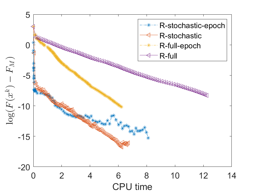
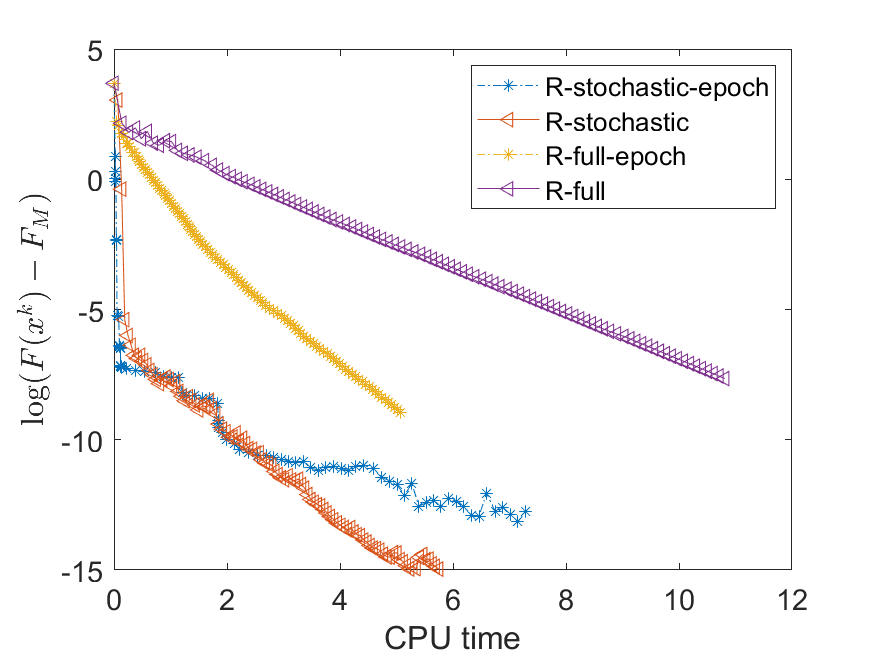
Figure 1: The performance profiles of our four algorithms on SPCA with $m=5000,n=200$ and $\mu=0.4$, left: $r=5$; right: $r=10$.

Table 1: The results of our algorithm compared with other algorithms on the sparse PCA problem with random data. The row labeled “Percentage” indicates the ratio of the algorithm is dominant in CPU time among all compared algorithms. The values of bold mean the optimal performance among all algorithms.

$(n,r,\mu)$	Objective function value				CPU time
	R-stochastic	ManPG	ManPG-A	R-sub	R-stochastic	ManPG	ManPG-A	R-sub
(200,10,0.04)	-1.988e+1	-1.988e+1	-1.988e+1	-1.018e+1	0.21	0.36	0.18	2.65
(200,10,0.06)	-1.823e+1	-1.823e+1	-1.823e+1	-8.224e+0	0.35	0.58	0.28	2.66
(200,10,0.08)	-1.670e+1	-1.669e+1	-1.669e+1	-6.512e+0	0.41	0.48	0.25	2.67
(200,20,0.04)	-3.722e+1	-3.722e+1	-3.722e+1	-2.004e+1	4.69	3.84	2.04	5.88
(200,20,0.06)	-3.417e+1	-3.417e+1	-3.415e+1	-1.579e+1	2.50	5.75	2.76	5.60
(200,20,0.08)	-3.051e+1	-3.051e+1	-3.051e+1	-1.095e+1	1.19	2.83	1.28	6.01
(200,30,0.04)	-5.284e+1	-5.284e+1	-5.285e+1	-2.903e+1	1.37	6.38	3.41	9.62
(200,30,0.06)	-4.806e+1	-4.822e+1	-4.814e+1	-2.291e+1	7.00	12.31	4.56	10.03
(200,30,0.08)	-4.383e+1	-4.383e+1	-4.400e+1	-1.662e+1	0.83	6.27	4.74	10.37
(200,40,0.04)	-6.618e+1	-6.618e+1	-6.613e+1	-3.715e+1	10.04	14.94	4.93	14.92
(200,40,0.06)	-6.071e+1	-6.078e+1	-6.078e+1	-2.969e+1	10.73	14.02	6.53	14.35
(200,40,0.08)	-5.528e+1	-5.527e+1	-5.528e+1	-2.093e+1	3.89	16.18	7.18	14.84
(200,50,0.04)	-7.904e+1	-7.908e+1	-7.905e+1	-4.450e+1	13.75	31.19	10.10	22.85
(200,50,0.06)	-7.193e+1	-7.192e+1	-7.189e+1	-3.480e+1	2.59	27.55	7.27	23.98
(200,50,0.08)	-6.542e+1	-6.543e+1	-6.553e+1	-2.504e+1	16.40	22.24	13.43	23.45
(300,10,0.04)	-2.351e+1	-2.351e+1	-2.351e+1	-1.160e+1	0.12	0.43	0.23	4.25
(300,10,0.06)	-2.152e+1	-2.152e+1	-2.152e+1	-9.712e+0	2.99	0.76	0.36	4.12
(300,10,0.08)	-1.948e+1	-1.951e+1	-1.951e+1	-7.184e+0	3.84	1.05	0.49	4.18
(300,20,0.04)	-4.422e+1	-4.428e+1	-4.428e+1	-2.337e+1	4.66	2.45	1.46	7.17
(300,20,0.06)	-4.038e+1	-4.036e+1	-4.036e+1	-1.803e+1	0.95	3.43	1.75	7.19
(300,20,0.08)	-3.634e+1	-3.634e+1	-3.640e+1	-1.412e+1	1.67	3.87	2.80	7.33
(300,30,0.04)	-6.340e+1	-6.340e+1	-6.336e+1	-3.347e+1	3.77	12.17	3.90	14.65
(300,30,0.06)	-5.702e+1	-5.702e+1	-5.709e+1	-2.685e+1	10.32	10.34	5.87	14.33
(300,30,0.08)	-5.171e+1	-5.171e+1	-5.171e+1	-1.878e+1	1.54	9.67	4.48	14.66
(300,40,0.04)	-8.068e+1	-8.068e+1	-8.074e+1	-4.385e+1	1.19	12.95	10.10	19.33
(300,40,0.06)	-7.266e+1	-7.266e+1	-7.269e+1	-3.235e+1	8.45	18.43	8.51	19.87
(300,40,0.08)	-6.595e+1	-6.594e+1	-6.613e+1	-2.479e+1	3.25	13.16	11.99	19.56
(300,50,0.04)	-9.606e+1	-9.605e+1	-9.608e+1	-5.353e+1	2.41	25.50	16.59	26.65
(300,50,0.06)	-8.703e+1	-8.724e+1	-8.713e+1	-4.047e+1	16.81	52.02	20.25	26.74
(300,50,0.08)	-7.826e+1	-7.826e+1	-7.804e+1	-2.851e+1	5.34	39.97	11.42	31.45
(500,10,0.04)	-3.056e+1	-3.056e+1	-3.056e+1	-1.692e+1	0.62	1.55	0.85	10.42
(500,10,0.06)	-2.757e+1	-2.757e+1	-2.757e+1	-1.362e+1	1.43	1.40	0.69	10.44
(500,10,0.08)	-2.473e+1	-2.476e+1	-2.476e+1	-1.070e+1	8.15	1.16	0.67	10.79
(500,20,0.04)	-5.820e+1	-5.820e+1	-5.817e+1	-3.254e+1	2.44	5.40	2.95	17.92
(500,20,0.06)	-5.196e+1	-5.196e+1	-5.196e+1	-2.543e+1	0.68	2.90	1.68	18.26
(500,20,0.08)	-4.649e+1	-4.649e+1	-4.652e+1	-1.895e+1	2.97	5.74	4.32	19.35
(500,30,0.04)	-8.199e+1	-8.199e+1	-8.189e+1	-4.672e+1	4.53	20.92	6.13	31.88
(500,30,0.06)	-7.443e+1	-7.446e+1	-7.450e+1	-3.727e+1	16.30	9.26	6.35	29.98
(500,30,0.08)	-6.724e+1	-6.723e+1	-6.729e+1	-2.682e+1	2.70	15.76	8.49	30.34
(500,40,0.04)	-1.060e+2	-1.060e+2	-1.060e+2	-5.875e+1	7.79	30.92	20.98	38.18
(500,40,0.06)	-9.557e+1	-9.557e+1	-9.554e+1	-4.867e+1	3.90	45.70	13.98	38.03
(500,40,0.08)	-8.492e+1	-8.492e+1	-8.499e+1	-3.362e+1	3.91	36.98	21.05	37.90
(500,50,0.04)	-1.271e+2	-1.271e+2	-1.272e+2	-7.299e+1	8.67	29.91	20.22	52.52
(500,50,0.06)	-1.140e+2	-1.140e+2	-1.142e+2	-5.714e+1	4.21	39.19	29.72	52.59
(500,50,0.08)	-1.025e+2	-1.025e+2	-1.024e+2	-4.153e+1	12.17	57.37	26.65	53.36
Percentage					64.44%	0	35.56%	0

5.2 Compressed modes in Physics

In physics, the compressed modes (CMs) problem seeks spatially localized solutions of the independent-particle Schrödinger equation:

$$\hat{H}\phi(x)=\lambda\phi(x),~{}~{}x\in\Omega,$$ (5.5)

where $\hat{H}=-\frac{1}{2}\Delta$ and $\Delta$ is a Laplacian operator. Consider the $1$-D free-electron (FE) model with $\hat{H}=-\frac{1}{2}\partial_{x^{2}}$ in our experiments. By proper discretization, the CMs can be reformulated to

$$\min_{X\in\mathbb{R}^{n\times r}}\mathrm{tr}(X^{T}HX)+\mu\|X\|_{1},~{}~{}\mbox{s.t. }~{}~{}X^{T}X=I_{r},$$ (5.6)

where $H$ is the discretized Schrödinger operator, $\mu$ is a regularization parameter. The interesting readers are referred to ozolicnvs2013compressed for more details. In our experiments, we use the polar decomposition as the retraction mapping. The domain $\Omega:=[0,50]$ is discretized with $n$ equally spaced nodes. Since CMs problem (5.6) is not of finite-sum form, we only compare the results of the R-full-epoch algorithm (abbreviated as R-F-epo) with other algorithms. Table LABEL:tab:cms_s1 presents the objective function value and CPU time of the algorithms on CMs problem with different values of $(n,r,\mu)$. Our algorithm outperforms other algorithms in most cases.

Table 2: The results of our algorithm compared with other algorithms on CMs with random data. The row labeled “Percentage” indicates the ratio of the algorithm is dominant in CPU time among all compared algorithms.

$(n,r,\mu)$	Objective function value				CPU time
	R-F-epo	ManPG	ManPG-A	R-sub	R-F-epo	ManPG	ManPG-A	R-sub
(128,5,0.1)	1.355e+0	1.355e+0	1.355e+0	1.360e+0	0.25	0.55	0.48	2.15
(128,5,0.1)	2.356e+0	2.356e+0	2.356e+0	2.361e+0	1.06	0.21	0.14	2.38
(128,5,0.2)	4.097e+0	4.097e+0	4.097e+0	4.118e+0	0.58	0.01	0.01	2.32
(128,5,0.3)	5.661e+0	5.661e+0	5.661e+0	5.705e+0	0.64	0.08	0.05	2.41
(128,10,0.1)	2.937e+0	2.937e+0	2.937e+0	2.940e+0	1.09	1.41	0.95	4.07
(128,10,0.1)	4.815e+0	4.815e+0	4.815e+0	4.824e+0	1.50	1.44	2.20	6.12
(128,10,0.2)	8.206e+0	8.206e+0	8.206e+0	8.250e+0	0.97	3.85	3.04	6.03
(128,10,0.3)	1.133e+1	1.133e+1	1.133e+1	1.142e+1	3.53	1.03	1.13	4.20
(128,15,0.1)	5.374e+0	5.375e+0	5.375e+0	5.376e+0	0.18	2.85	3.13	6.50
(128,15,0.1)	8.012e+0	8.012e+0	8.012e+0	8.028e+0	0.88	6.24	6.47	7.79
(128,15,0.2)	1.282e+1	1.282e+1	1.282e+1	1.287e+1	0.49	3.12	3.11	6.72
(128,15,0.3)	1.726e+1	1.726e+1	1.726e+1	1.739e+1	0.76	1.66	1.67	6.69
(128,20,0.1)	9.184e+0	9.184e+0	9.184e+0	9.184e+0	0.74	17.58	24.86	16.65
(128,20,0.1)	1.253e+1	1.253e+1	1.253e+1	1.254e+1	4.32	11.42	9.74	12.64
(128,20,0.2)	1.861e+1	1.861e+1	1.861e+1	1.869e+1	5.10	4.25	3.75	12.19
(128,20,0.3)	2.429e+1	2.429e+1	2.429e+1	2.447e+1	4.77	11.97	10.86	12.72
(128,30,0.1)	2.270e+1	2.270e+1	2.269e+1	2.270e+1	0.58	78.95	115.97	19.96
(128,30,0.1)	2.737e+1	2.737e+1	2.737e+1	2.738e+1	0.65	59.77	81.07	29.15
(128,30,0.2)	3.575e+1	3.575e+1	3.575e+1	3.584e+1	1.29	6.53	6.82	21.06
(128,30,0.3)	4.375e+1	4.375e+1	4.375e+1	4.395e+1	0.58	3.69	3.33	20.62
(256,5,0.1)	1.788e+0	1.788e+0	1.788e+0	1.790e+0	0.13	0.29	0.13	2.69
(256,5,0.1)	3.113e+0	3.113e+0	3.113e+0	3.124e+0	0.38	1.13	0.88	2.66
(256,5,0.2)	5.416e+0	5.416e+0	5.416e+0	5.461e+0	0.59	0.24	0.23	2.70
(256,5,0.3)	7.489e+0	7.489e+0	7.489e+0	7.592e+0	0.31	0.03	0.02	3.35
(256,10,0.1)	3.747e+0	3.747e+0	3.747e+0	3.752e+0	0.38	5.07	3.15	5.44
(256,10,0.1)	6.273e+0	6.273e+0	6.273e+0	6.291e+0	0.86	2.86	3.53	6.35
(256,10,0.2)	1.084e+1	1.084e+1	1.084e+1	1.095e+1	2.69	22.63	18.98	5.85
(256,10,0.3)	1.498e+1	1.498e+1	1.498e+1	1.519e+1	0.59	1.37	1.68	5.64
(256,15,0.1)	6.522e+0	6.522e+0	6.522e+0	6.528e+0	0.78	7.75	5.32	8.67
(256,15,0.1)	1.010e+1	1.010e+1	1.010e+1	1.013e+1	1.05	4.17	3.62	9.42
(256,15,0.2)	1.659e+1	1.659e+1	1.659e+1	1.672e+1	2.24	9.36	18.29	8.91
(256,15,0.3)	2.259e+1	2.259e+1	2.259e+1	2.294e+1	2.72	14.02	25.48	8.42
(256,20,0.1)	1.068e+1	1.068e+1	1.068e+1	1.069e+1	0.71	24.35	24.07	13.79
(256,20,0.1)	1.522e+1	1.522e+1	1.522e+1	1.526e+1	1.46	12.17	14.15	15.48
(256,20,0.2)	2.350e+1	2.350e+1	2.350e+1	2.368e+1	4.72	22.24	18.79	15.84
(256,20,0.3)	3.121e+1	3.121e+1	3.121e+1	3.160e+1	0.91	14.40	15.64	13.94
(256,30,0.1)	2.509e+1	2.509e+1	2.509e+1	2.510e+1	0.82	59.27	66.48	24.45
(256,30,0.1)	3.149e+1	3.149e+1	3.149e+1	3.152e+1	0.41	35.48	41.17	24.90
(256,30,0.2)	4.308e+1	4.308e+1	4.308e+1	4.330e+1	0.59	18.60	19.30	27.87
(256,30,0.3)	5.391e+1	5.391e+1	5.391e+1	5.447e+1	0.62	31.60	26.37	24.85
Percentage					77.5%	7.5%	17.50%	0

6 Conclusions

In this paper, we present a novel family of Riemannian gradient-based methods, namely Riemannian smoothing gradient and Riemannian smoothing stochastic gradient, designed to identify generalized $\epsilon$-stationarity points for a class of nonconvex and nonsmooth problems on compact Riemannian submanifold embedded in Euclidean space. We introduce the concept of generalized $\epsilon$-stationarity, which extends the notion of $\epsilon$-stationarity. By leveraging the Moreau envelope with a sequence of decreasing smoothing parameters, we transform the problem into a smoothed formulation in Euclidean space. We establish the smoothness of this problem on the Riemannian compact submanifold. We demonstrate that our proposed algorithms exhibit iteration complexities of $\mathcal{O}(\epsilon^{-3})$ and $\mathcal{O}(\epsilon^{-5})$ to achieve a generalized $\epsilon$-stationarity, respectively. Notably, our algorithms outperform other existing methods in numerical experiments conducted on both the SPCA and CMs problems.

Declarations

This research was supported by the Natural Science Foundation of China with grant 12071398, the Natural Science Foundation of Hunan Province with grant 2020JJ4567, and the Key Scientific Research Found of Hunan Education Department with grants 20A097 and 18A351. The authors have no relevant financial or non-financial interests to disclose.

References

- \bibcommenthead
- (1) Jolliffe, I.T., Trendafilov, N.T., Uddin, M.: A modified principal component technique based on the LASSO. Journal of computational and Graphical Statistics 12(3), 531–547 (2003)
- (2) Selvan, S.E., Borckmans, P.B., Chattopadhyay, A., Absil, P.-A.: Spherical mesh adaptive direct search for separating quasi-uncorrelated sources by range-based independent component analysis. Neural computation 25(9), 2486–2522 (2013)
- (3) Selvan, S.E., George, S.T., Balakrishnan, R.: Range-based ICA using a nonsmooth quasi-Newton optimizer for electroencephalographic source localization in focal epilepsy. Neural computation 27(3), 628–671 (2015)
- (4) Deng, K., Hu, J.: Decentralized projected riemannian gradient method for smooth optimization on compact submanifolds. arXiv preprint arXiv:2304.08241 (2023)
- (5) Cambier, L., Absil, P.-A.: Robust low-rank matrix completion by Riemannian optimization. SIAM Journal on Scientific Computing 38(5), 440–460 (2016)
- (6) Hosseini, S., Uschmajew, A.: A Riemannian gradient sampling algorithm for nonsmooth optimization on manifolds. SIAM Journal on Optimization 27(1), 173–189 (2017)
- (7) Absil, P.-A., Hosseini, S.: A collection of nonsmooth Riemannian optimization problems, pp. 1–15 (2019). https://doi.org/10.1007/978-3-030-11370-4_1. Springer
- (8) Luenberger, D.G.: The gradient projection method along geodesics. Management Science 18(11), 620–631 (1972)
- (9) Boumal, N., Absil, P.-A., Cartis, C.: Global rates of convergence for nonconvex optimization on manifolds. IMA Journal of Numerical Analysis 39(1), 1–33 (2019)
- (10) Absil, P.-A., Baker, C.G., Gallivan, K.A.: Trust-region methods on Riemannian manifolds. Foundations of Computational Mathematics 7(3), 303–330 (2007)
- (11) Huang, W., Absil, P.-A., Gallivan, K.A.: A Riemannian BFGS method without differentiated retraction for nonconvex optimization problems. SIAM Journal on Optimization 28(1), 470–495 (2018)
- (12) Hu, J., Milzarek, A., Wen, Z., Yuan, Y.-x.: Adaptive quadratically regularized Newton method for Riemannian optimization. SIAM Journal on Matrix Analysis and Applications 39(3), 1181–1207 (2018)
- (13) Kovnatsky, A., Glashoff, K., Bronstein, M.M.: MADMM: a generic algorithm for non-smooth optimization on manifolds. In: Computer Vision–ECCV 2016: 14th European Conference, Amsterdam, The Netherlands, October 11-14, 2016, Proceedings, Part V 14, pp. 680–696 (2016). Springer
- (14) Deng, K., Peng, Z.: A manifold inexact augmented Lagrangian method for nonsmooth optimization on Riemannian submanifolds in Euclidean space. IMA Journal of Numerical Analysis 43(3), 1653–1684 (2023)
- (15) Bonnabel, S.: Stochastic gradient descent on riemannian manifolds. IEEE Transactions on Automatic Control 58(9), 2217–2229 (2013)
- (16) Sato, H., Kasai, H., Mishra, B.: Riemannian stochastic variance reduced gradient algorithm with retraction and vector transport. SIAM Journal on Optimization 29(2), 1444–1472 (2019)
- (17) Shah, S.M.: Stochastic approximation on Riemannian manifolds. Applied Mathematics & Optimization 83, 1123–1151 (2021)
- (18) Boumal, N.: An Introduction to Optimization on Smooth Manifolds. Cambridge University Press, Cambridge, England (2023). https://doi.org/10.1017/9781009166164
- (19) Sato, H.: Riemannian Optimization and Its Applications. Springer, Cham (2021). https://doi.org/10.1007/978-3-030-62391-3
- (20) Hu, J., Liu, X., Wen, Z.-W., Yuan, Y.-X.: A brief introduction to manifold optimization. Journal of the Operations Research Society of China 8, 199–248 (2020)
- (21) Hosseini, S., Huang, W., Yousefpour, R.: Line search algorithms for locally Lipschitz functions on Riemannian manifolds. SIAM Journal on Optimization 28(1), 596–619 (2018)
- (22) de Carvalho Bento, G., da Cruz Neto, J.X., Oliveira, P.R.: A new approach to the proximal point method: convergence on general Riemannian manifolds. Journal of Optimization Theory and Applications 168(3), 743–755 (2016)
- (23) Ferreira, O., Oliveira, P.: Proximal point algorithm on Riemannian manifolds. Optimization 51(2), 257–270 (2002)
- (24) Böhm, A., Wright, S.J.: Variable smoothing for weakly convex composite functions. Journal of optimization theory and applications 188(3), 628–649 (2021)
- (25) Lin, Q., Chen, X., Peña, J.: A smoothing stochastic gradient method for composite optimization. Optimization Methods and Software 29(6), 1281–1301 (2014)
- (26) Xu, Y., Yan, Y., Lin, Q., Yang, T.: Homotopy smoothing for non-smooth problems with lower complexity than . In: Advances in Neural Information Processing Systems, vol. 29, pp. 1208–1216 (2016)
- (27) Wei, X., Yu, H., Ling, Q., Neely, M.: Solving non-smooth constrained programs with lower complexity than : A primal-dual homotopy smoothing approach. In: Advances in Neural Information Processing Systems, vol. 31, pp. 3995–4005 (2018)
- (28) Boţ, R.I., Böhm, A.: Variable smoothing for convex optimization problems using stochastic gradients. Journal of Scientific Computing 85(2), 33 (2020)
- (29) Metel, M., Takeda, A.: Simple stochastic gradient methods for non-smooth non-convex regularized optimization. In: Proceedings of the 36th International Conference on Machine Learning, vol. 97, pp. 4537–4545 (2019). PMLR
- (30) Chambolle, A., Pock, T.: A first-order primal-dual algorithm for convex problems with applications to imaging. Journal of mathematical imaging and vision 40(1), 120–145 (2011)
- (31) Ouyang, H., Gray, A.: Stochastic smoothing for nonsmooth minimizations: Accelerating sgd by exploiting structure. arXiv preprint arXiv:1205.4481 (2012)
- (32) Tran-Dinh, Q.: Adaptive smoothing algorithms for nonsmooth composite convex minimization. Computational Optimization and Applications 66(3), 425–451 (2017)
- (33) Liu, C., Boumal, N.: Simple algorithms for optimization on Riemannian manifolds with constraints. Applied Mathematics & Optimization 82(3), 949–981 (2020)
- (34) Qu, Q., Li, X., Zhu, Z.: A nonconvex approach for exact and efficient multichannel sparse blind deconvolution. In: Advances in Neural Information Processing Systems, vol. 32, pp. 4015–4026 (2019)
- (35) Zhang, C., Chen, X., Ma, S.: A Riemannian smoothing steepest descent method for non-lipschitz optimization on submanifolds. arXiv preprint arXiv:2104.04199 (2021)
- (36) Beck, A., Rosset, I.: A dynamic smoothing technique for a class of nonsmooth optimization problems on manifolds. SIAM Journal on Optimization 33(3), 1473–1493 (2023). https://doi.org/10.1137/22M1489447
- (37) Li, X., Chen, S., Deng, Z., Qu, Q., Zhu, Z., Man-Cho So, A.: Weakly convex optimization over Stiefel manifold using Riemannian subgradient-type methods. SIAM Journal on Optimization 31(3), 1605–1634 (2021)
- (38) Chen, S., Ma, S., Man-Cho So, A., Zhang, T.: Proximal gradient method for nonsmooth optimization over the Stiefel manifold. SIAM Journal on Optimization 30(1), 210–239 (2020)
- (39) Seguin, A., Kressner, D.: Continuation methods for riemannian optimization. SIAM Journal on Optimization 32(2), 1069–1093 (2022)
- (40) Li, J., Ma, S., Srivastava, T.: A Riemannian ADMM. arXiv preprint arXiv:2211.02163 (2022)
- (41) Absil, P.-A., Mahony, R., Sepulchre, R.: Optimization Algorithms on Matrix Manifolds, p. 224. Princeton University Press, Princeton, NJ (2008)
- (42) Zhang, J., Lin, H., Jegelka, S., Sra, S., Jadbabaie, A.: Complexity of finding stationary points of nonconvex nonsmooth functions. In: Proceedings of the 37th International Conference on Machine Learning, vol. 119, pp. 11173–11182 (2020). PMLR
- (43) Wang, Y., Yin, W., Zeng, J.: Global convergence of ADMM in nonconvex nonsmooth optimization. Journal of Scientific Computing 78(1), 29–63 (2019)
- (44) Themelis, A., Patrinos, P.: Douglas–Rachford splitting and ADMM for nonconvex optimization: Tight convergence results. SIAM Journal on Optimization 30(1), 149–181 (2020)
- (45) Ozoliņš, V., Lai, R., Caflisch, R., Osher, S.: Compressed modes for variational problems in mathematics and physics. Proceedings of the National Academy of Sciences 110(46), 18368–18373 (2013)