The CARMENES search for exoplanets around M dwarfs

It is clearly established that the Sun has an 11-year cycle that is caused by its internal magnetic field. This cycle is also observed in a sample of M dwarfs. In the framework of exoplanet detection or atmospheric characterisation of exoplanets, the activity status of the host star plays a crucial role, and inactive states are preferable for such studies. This means that it is important to know the activity cycles of these stars. We study systematic long-term variability in a sample of 211 M dwarfs observed with CARMENES, the high-resolution optical and near-infrared spectrograph at Calar Alto Observatory. In an automatic search using time series of different activity indicators, we identified 26 stars with linear or quadratic trends or with potentially cyclic behaviour. Additionally, we performed an independent search in archival R${}^{\prime}_{\rm HK}$  data collected from different instruments whose time baselines were usually much longer. These data are available for a subset of 186 of our sample stars. Our search revealed 22 cycle candidates in the data. We found that the percentage of stars showing long-term variations drops dramatically to the latest M dwarfs. Moreover, we found that the pseudo-equivalent width (pEW) of the H$\alpha$ and Ca ii infrared triplet more often triggers automatic detections of long-term variations than the TiO index, differential line width, chromatic index, or radial velocity. This is in line with our comparison of the median relative amplitudes of the different indicators. For stars that trigger our automatic detection, this leads to the highest amplitude variation in R${}^{\prime}_{\rm HK}$   , followed by pEW(H$\alpha$), pEW(Ca ii IRT), and the TiO index.

1 Introduction

Stellar activity is driven by an underlying magnetic dynamo that is predicted to change periodically according to the theory of an $\alpha$-$\Omega$ dynamo (Roberts & Stix, 1972). Dynamo simulations for the fully convective M dwarf Proxima Centauri also directly led to magnetic cycles (Yadav et al., 2016). This periodic behaviour manifests itself as stellar activity cycles. These cycles have also been observed on stars other than the Sun by time series of X-ray and chromospheric activity indicators, or photometry. While the Sun varies in X-rays as a coronal indicator by more than a factor of ten during its cycle (Peres et al., 2000), only a few stars have been found to exhibit long-term cyclic behaviour in X-rays. These cycles all had a much lower amplitude (Robrade et al., 2012; Wargelin et al., 2017; Coffaro et al., 2020).

Chromospheric indicators, on the other hand, have been used widely for a cycle search in solar-type stars. The monitoring program conducted at the Mt. Wilson Observatory (Wilson, 1978) using the line index of the Ca ii H & K lines revealed that stellar activity cycles are a ubiquitous phenomenon (Baliunas et al., 1995). Short and long cycles have been found for several stars (Brandenburg et al., 2017), starting with the Sun, which exhibits the approximately 80-year-long Gleissberg cycle (Gleissberg, 1945) and the 11-year-long Schwabe cycle (Richards et al., 2009), although it also shows a transient periodic behaviour of about one-half to two years (Ballester et al., 2002; Mursula et al., 2003). Multiple cycles have also been found in other stars, such as in $\epsilon$ Eridani, which displays two distinct cycles at about three and twelve years (Brandenburg et al., 2017; Jeffers et al., 2022b). In addition to these decade-long cycles, F-type stars with activity cycles shorter than one year have been revealed (Jeffers et al., 2018; Mittag et al., 2019). Although some authors sort different cycles lengths into an inactive and active branch, the existence of these two branches has been questioned by Boro Saikia et al. (2018) and Brown et al. (2022), for example.

While extensive work about activity cycles has been conducted on FGK stars (see e.g. Lovis et al. (2011)), only a few M dwarfs have been under investigation, mostly using photometric time series. For example, Suárez Mascareño et al. (2016) derived magnetic cycles and rotation periods in 125 late-type stars, 70 of which were M dwarfs. About half of them exhibited long-term photometric variability. Another study that used photometric data to derive rotation periods and cycles was conducted by Díez Alonso et al. (2019). They found 12 stars with long-term cyclic variations with an observation time baseline of more than nine years. Moreover, Küker et al. (2019) found that in a sample of 31 M dwarfs, 19 exhibited a cycle. Using chromospheric indicators, fewer cycles were found for M dwarfs by Robertson et al. (2013) by employing time series of H$\alpha$ indices. They also identified linear and quadratic trends as possible parts of activity cycles, which are too long to be covered by the available data. While they searched 93 K and M dwarfs, only six periods and seven long-term trends were identified by Robertson et al. (2013). Using H$\alpha$ and Ca ii H&K data, Suárez Mascareño et al. (2018) found that in a sample of 71 M dwarfs, 13 exhibited a cycle. Moreover, Gomes da Silva et al. (2012) found a correlation between long-term activity variations measured by a Na i D index and radial velocity (RV) in about one-third of the 27 stars they analysed.

This long-term correlation between an activity indicator and RV may impose problems for exoplanet detections with longer orbital periods, as is already known from short time-activity variations caused by the rotation period of the star, for instance, which may hide or mimic a planetary RV signal (Queloz et al., 2001; Dumusque et al., 2011; Jeffers et al., 2022a). This is caused by the asymmetry that is imprinted on the spectrum by surface heterogeneities. The asymmetry in turn leads to a shift of the line centre depending on the size and location of the active region on the stellar surface. Accordingly, Stock et al. (2020) found a long-term periodic behaviour in their RV measurements, which were mainly conducted with the CARMENES spectrograph. In the framework of an exoplanet search, they found tentative activity cycles of 600 and 2900 d for the two M dwarfs GJ 251 and Lalande 21185, respectively.

This study searches for more activity cycles in M dwarfs using data from the CARMENES spectrograph for different chromospheric line measurements. The paper is structured as follows: In Sect. 2 we present the data, their reduction, and the method for the measurement of our chromospheric indicators. In Sect. 3 we detail our search methods for activity cycles and trends. In Sect. 4 we present and discuss our results. We give a summary and concluding remarks in Sect. 5.

2 Observations and measurements of chromospheric indicators

All spectra used for the present analysis were taken with the CARMENES spectrograph, installed at the 3.5 m Calar Alto telescope (Quirrenbach et al., 2020). CARMENES is a spectrograph covering the wavelength range from 5200 to 9600 Å  in the visual channel (VIS) and from 9600 to 17 100 Å  in the near-infrared channel (NIR). The instrument provides a spectral resolution of $\sim$ 94 600 in VIS and $\sim$ 80 400 in NIR. The CARMENES consortium is conducting a survey of $\sim$350 M dwarfs to find low-mass exoplanets (Alonso-Floriano et al., 2015; Reiners et al., 2018). Since the cadence of the spectra is optimised for the planet search, usually no continuous time series are obtained.

2.1 Data reduction and sample construction

In our analysis, we considered a sample of 362 M dwarfs observed by CARMENES, resulting in more than 19 000 spectra taken before February 2022. From this sample, we excluded known binaries (Baroch et al., 2018; Schweitzer et al., 2019; Baroch et al., 2021). Binaries may hamper our analysis because the line shifts induced by binarity may be large enough to shift parts of the line out of the integration range for line indices or pseudo-equivalent width (pEW). Additionally, we had to constrain the stellar sample further because the CARMENES data are optimised for exoplanetary search, and therefore not all stars are observed with the same frequency or time baseline (i.e. the elapsed time between the first and last observation). We wish to search for long-term systematic variations, therefore we restricted the sample to all stars with a time coverage of more than 200 days with at least 20 observations to allow for a statistically meaningful analysis. Even though it is hard to detect periods with so few observations, linear and quadratic trends may still be detected. In this fashion, we obtained a sub-sample of 211 stars for our analysis. We show the distribution of the observation time baseline for these 211 stars in Fig. 1.

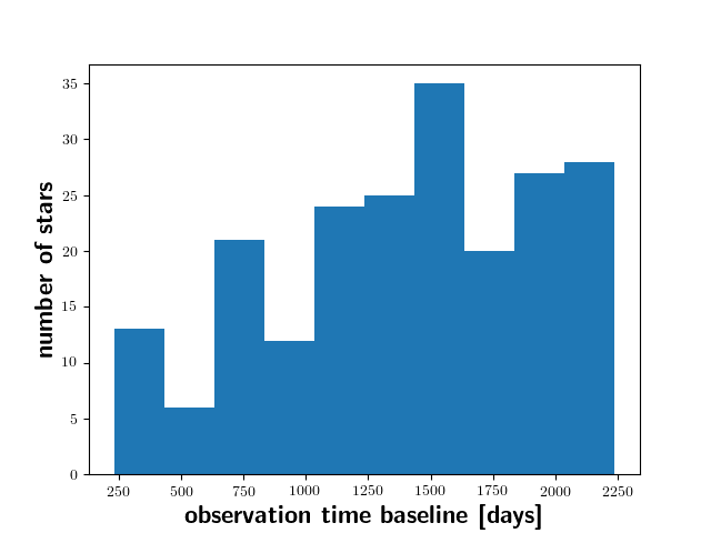
Figure 1: Distribution of the observation time baseline for our sample of 211 stars with more than 19 observations and a minimum observation time baseline of 200 days.

The stellar spectra were reduced using the CARMENES reduction pipeline (Zechmeister et al., 2014; Caballero et al., 2016). Subsequently, we corrected them for barycentric and RV motions and carried out a correction for telluric absorption lines (Nagel et al., 2019) using the molecfit package. No correction for airglow emission lines was attempted because they do not play a role for the activity indicators we used.

2.2 Measurement of activity indicators

To assess the activity state of the stars in each spectrum, we employed pEW measurements because the spectra of M dwarfs do not show an identifiable continuum (because molecular absorption lines are present nearly everywhere). We measured the pEW of the blue Ca ii infrared triplet (IRT) line at 8500.35 Å  (hereafter Ca ii IRT₁) and of the middle Ca ii IRT line at 8544.44 Å  (hereafter Ca ii IRT₂), and the H$\alpha$ line (all wavelengths are given for vacuum conditions). The three Ca ii IRT  lines act very similarly regarding activity (Lafarga et al., 2021), therefore we used only the two bluer lines because they are located on the same order as the spectrograph.

The pEW was calculated using the expression

$$\mathrm{pEW}=\int(1-F_{\rm core}/F_{0})d\lambda,$$ (1)

where $F_{core}$ is the flux density in the line band, $F_{0}$ is the mean flux density in the two reference intervals (representing the pseudo-continuum), and $\lambda$ denotes the wavelength. Thus, time series of pEW measurements were obtained for each star. The integration ranges for the individual lines are given in Table 1.

The uncertainty of individual pEW measurements depends on the S/N of the spectra, which can be particularly problematic for the H$\alpha$ line, where the S/N is typically better for bright, early M dwarfs than for fainter mid-type M dwarf. We did not compute pEWs when the S/N in the pseudo-continuum was lower than 15. Therefore, no pEW(H$\alpha$) measurements could be obtained for some of the latest and faintest M dwarfs, and we omitted these stars from further analysis when fewer than 20 measurements were available. When the S/N was good enough to compute pEWs, we calculated their error by a bootstrap analysis using the flux density errors from the pipeline to re-compute the pEWs 1000 times. This yielded quite low statistical errors; in the case of pEW(H$\alpha$) and pEW(Ca ii IRT), the relative statistical error is about $10^{-7}$–$10^{-5}$ for most of the spectra, while the time series of the chromospheric indicators of inactive stars exhibits a larger scatter of about 10% of the median value of the pEW in H$\alpha$ and of 3% in both pEW(Ca ii IRT). This is apparently caused by intrinsic variations of the activity level of the stars, and we therefore applied this as error to all chromospheric indicator measurements. We also display this scatter as error bars in all the figures showing time series.

In addition to these classical chromospheric indicators, we also considered more recently introduced activity indicators, specifically, a TiO index defined as the ratio of the average flux density in a band red- and blue-wards of the band head, as introduced by Schöfer et al. (2019). The wavelength bands, which slightly differ from Schöfer et al. (2019), are given in Table 1. An error was again estimated by the variation in inactive stars to be 0.3% (which roughly agrees with a bootstrap analysis in this case). Moreover, we used RV, chromatic index (CRX; as a measure of change in RV shift as a function of wavelength), and the differential line width (dLw; as a measure of changes in line width compared to a constructed average). All three indicators and their errors were obtained for the VIS arm of CARMENES from the reduction pipeline serval (Zechmeister et al., 2018). They have been used for example in a search for rotation periods by Lafarga et al. (2021).

Table 1: Parameters (vacuum wavelength) of the pEW and TiO index calculation.

Line	Wave-	Width	Reference	Reference
	length		band 1	band 2
	[Å]	[Å]	[Å]	[Å]
H$\alpha$	6564.60	1.60	6537.4–6547.9	6577.9–6586.4
Ca ii IRT1	8500.35	0.50	8476.3–8486.3	8552.4–8554.4
Ca ii IRT2	8544.44	0.50	8476.3–8486.3	8552.4–8554.4
TiO			7056.2–7059.2	7046.0–7050.0

For a sub-sample of 186 stars with R${}^{\prime}_{\rm HK}$ measurements compiled by Perdelwitz et al. (2021) from seven different instruments (most spectra were obtained with the HARPS, HIRES, and Narval spectrographs), we included these data in our cycle search. Perdelwitz et al. (2021) used the pipeline-reduced spectra from the respective archives and computed the chromospheric line fluxes in the Ca ii H & K lines after rectification and subtraction of the photospheric flux using PHOENIX (Hauschildt et al., 1999) photospheric model spectra from the Husser et al. (2013) database. While some of the obtained R${}^{\prime}_{\rm HK}$ time series temporally overlap with the CARMENES data, most of them do not. Moreover, the observational cadence is usually coarser, while the time baseline is much longer than for the CARMENES data. This longer baseline makes the data more suitable for a cycle search.

2.3 Compilation of cycles from the literature

From the literature, we collected a list of 57 proposed cycles in 41 stars as linear or quadratic trends for our sample stars. Most of these cycles originate from an analysis of photometric data. For example, the studies by Suárez Mascareño et al. (2016), which were dedicated to a cycle search, and of Díez Alonso et al. (2019), where some cycles emerged as by-products of a rotation period search, used only photometric data. We also included cycles found in photometric data by Küker et al. (2019). In contrast, Robertson et al. (2013) used an H$\alpha$ index for an activity cycle search, and Perdelwitz et al. (2021) also performed a period analysis on their R${}^{\prime}_{\rm HK}$ data with three published cycles. We also have some stars in common with the sample of Suárez Mascareño et al. (2018), who used the Ca ii H&K and H$\alpha$ index for their cycle search.

Other activity cycles have been published as part of RV exoplanet searches that also used the CARMENES data, for example by Stock et al. (2020) for Lalande 21185 (including RV data from the SOPHIE instrument) and GJ 251 (including data from the HARPS instrument), for which cycle lengths of 2900 days and 600 days were found. Moreover, Lopez-Santiago et al. (2020) found a probable cycle length of 14 years for the star GJ 3512 by performing a combined fit to the rotation period and activity cycle.

3 Searching for systematic long-term variations

We used several methods to search for systematic long-term variations in the available data to account for the different time scales involved. While we searched for cycles that were potentially longer than a decade, our longest time baseline is only 6.1 a (= years). This implies that we may cover only parts of activity cycles. Therefore, we also searched for linear and quadratic trends, which may arise when the data cover only the gradual decay or increase in activity or include an activity maximum or minimum. We caution, nevertheless, that these systematic long-term variations need not to lead to periodic behaviour. Therefore, we distinguish between periodic behaviour, where we do cover at least one full period, and linear and quadratic trends, which are indicative of systematic, but not necessarily cyclic behaviour.

Moreover, in all our search algorithms, we decided to tie a detection to at least three indicators and used in turn not as strict criteria for the individual indicators, as we would have applied if we had accepted detections for single indicators. We opted for this alternative since correlated (or anti-correlated) behaviour between the indicators is expected in the case of systematic long-term variability since they (optimally) all should react to the changing activity level. We decided in this context to use at least three indicators, because for only two indicators, the two used Ca ii IRT lines may trigger a detection alone. With more than three indicators, this criterion is very strict because it may lead to non-detections when the different indicators have different sensitivities.

Finally, before searching for cycles or parts of it, we applied a 3$\sigma$ clipping to each of the indicator time series using the python routine scipy.sigmaclip. Thus we avoided outliers caused by flaring, bad weather, or instrumental effects, which may confound the search. Moreover, after conducting the automatic variability search, we excluded all time series that had data gaps spanning more than 40% of the temporal baseline, were longer than 550 days, or both, because we noted visually that long data gaps like this were often problematic.

3.1 Searching for linear trends

The linear trend search was conducted as follows: We used each of the pEW of H$\alpha$, Ca ii IRT₁, Ca ii IRT₂, and the I_TiO  indices as well as CRX and dLw to compute a linear regression with respect to time, employing scipy.stats.linregress in python, which outputs also Pearson’s correlation coefficient $r$ and the corresponding $p$-value. This additional output allowed us to identify trends in time. These trends were searched for using the whole data set for each star because we are interested in finding stars for which the whole time series covers the activity increase or decrease phase of an activity cycle. The identified trends are linear by the definition of the Pearson’s correlation coefficient, but a subsequent visual inspection showed that in a few cases, the linear description only holds as a first-order approximation, but a parabolic description appears to be more appropriate. These time series were also found in our quadratic trend search and were marked accordingly. Therefore, we claim a linear trend when the Pearson correlation coefficients are abs$(r)>0.55$ and $p<0.002$ in three or more of the indicators. We determined these thresholds empirically using a test sample of 20 stars that included 3 stars whose linear trends were found by eye. The relatively low threshold of abs$(r)>0.55$ was justified a posteriori because we did not reject any of the automatically found trends by eye (but only found some to be better described by quadratic trends).

An instructive example of the trends we found is shown in Fig. 2 for the M1.0 V star J23245+578 / BD+57 2735. The pEW(H$\alpha$) and pEW(Ca ii IRT₁) both show about the same slope. This is the case for most of the trends we found. In one of the time series, we nevertheless found one convincing example in which the trends of H$\alpha$ and the pEW(Ca ii IRT₁) were of opposite sign. In the M0.0 V star J13450+176 / BD+18 2776, we found a highly significant Pearson correlation coefficient of 0.95 ($p$-value $10^{-15}$) between the the values of pEW(Ca ii IRT₁) and pEW(Ca ii IRT₂), while the correlation of the values of pEW(H$\alpha$) and the two pEW(Ca ii IRT) are $-0.73$ and $-0.69$, respectively ($p$-values $<3.1\cdot 10^{-5}$). We show the corresponding time series in Fig. 3 with the pEW(Ca ii IRT₂) instead of I_TiO as an exception. This behaviour may be explained by the relative inactivity of the star. With an increase in activity level in M dwarfs, we first expect a deepening of the H$\alpha$ line, which is followed by a fill-in, until the line finally enters emission at even higher activity levels (Cram & Mullan, 1979). For the Ca ii IRT lines, only a fill-in is expected instead. This behaviour can lead to an anti-correlation of the two lines for the lowest activity stars, where H$\alpha$ still deepens with increasing activity.

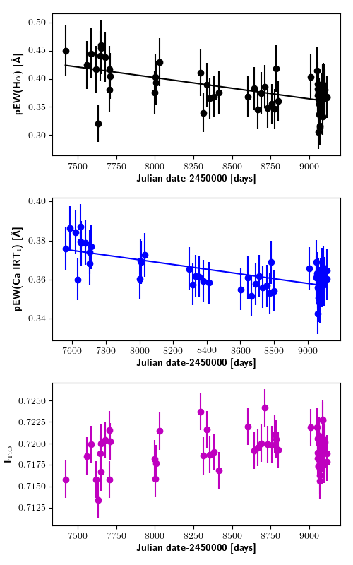
Figure 2: Time series of J23245+578 / BD+57 2735. We show the pEW(H$\alpha$) (top, black dots), pEW(Ca ii IRT₁) (middle, blue dots), and I_TiO  (bottom, magenta dots). Additionally, the best linear fit is indicated as the solid line. The error bars are not statistical, but determined by the activity jitter of inactive stars.

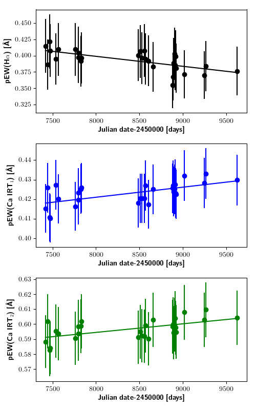
Figure 3: Time series of J13450+176 / BD+18 2776. We show the pEW(H$\alpha$) (top, black dots), pEW(Ca ii IRT₁) (middle, blue dots), and pEW(Ca ii IRT₂) (bottom, green dots). Additionally, the best-fit linear trend is indicated as the solid line.

3.2 Searching for quadratic trends

We used a parabolic fit to identify another type of systematic long-term variability. We applied a collection of ten criteria, nine of which had to be fulfilled to accept a quadratic trend. We used a reduced $\chi^{2}$ like quantity to access the quality of the fit. However, the correspondence is not exact owing to our use of a generic jitter estimate and the absence of the degrees of freedom in the definition: (i) $\chi^{2}=\frac{1}{n_{\mathrm{spec}}}\frac{\sum(pEW_{i}-poly)^{2}}{\sum err_{i}^{2}}<1.05$ for pEW(H$\alpha$) (ii-iii) The same holds for Ca ii IRT₁  and Ca ii IRT₂  with a threshold of 1.0 (iv) The same holds for the TiO index with a threshold of 1.03. To fine-tune these first four criteria, we visually inspected a sub-sample of 20 time series, which included five time series for which a quadratic trend was found by eye. (v)–(viii) All maxima or minima of the parabolic fit had to lie within the observed time baseline. (ix) The maximum difference between the corresponding dates of the maxima or minima of the quadratic fits of the different activity indicators must be lower than 15% of the observation time baseline and shorter than 150 days, with the exception of one indicator. (x) Same as (ix), but without any exception. These last two criteria make use of the expected correlated behaviour of the different indicators and at least (ix) must be triggered for an automatic detection.

As an instructive example of our quadratic trend search, we show the M0.0 V star J14257+236W / BD+24 2733A in Fig. 4. This clearly demonstrates the need of longer time baselines to clarify whether these quadratic trends lead to periodic behaviour or are just systematic episodes embedded in chaotic variations.

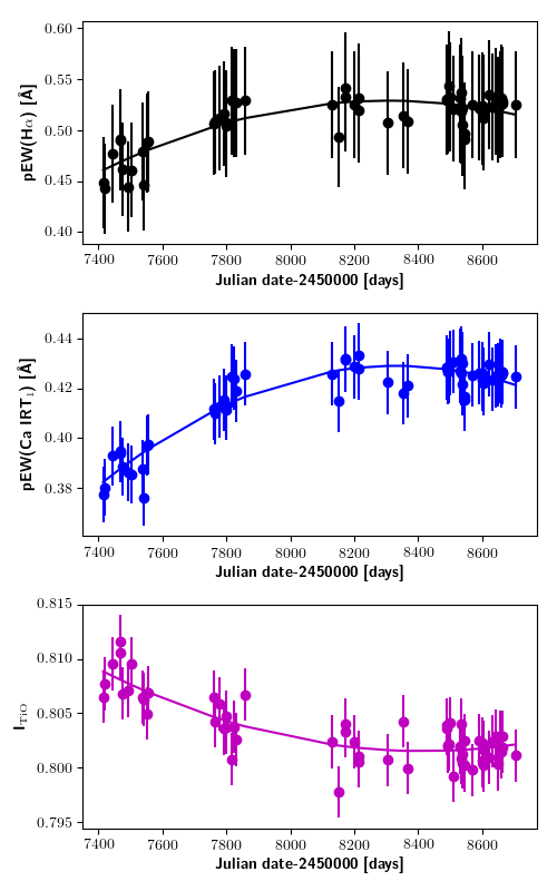
Figure 4: Time series of J14257+236W / BD+24 2733A. We show pEW(H$\alpha$) (top) and pEW(Ca ii IRT₁) (bottom). Additionally, the best-fit quadratic trend is indicated as the solid line.

3.3 Searching for cycles

To search for cyclic behaviour, we applied the generalised Lomb-Scargle (GLS) periodogram (Zechmeister & Kürster, 2009) as implemented in PyAstronomy (Czesla et al., 2019) to each of our chromospheric indicator time series, namely pEW(H$\alpha$), pEW(Ca ii IRT₁), pEW(Ca ii IRT₂), I_TiO, R${}^{\prime}_{\rm HK}$   (whenever available), RV, CRX, and dLw. In our further analysis, we searched for periods longer than one year and shorter than 90% of the time baseline of the individual data set to cover whole cycles. We accepted periods with an FAP lower than 0.1% as significant. When we found significant periods in three or more indicators, we verified whether the difference between the maximum peak periods of at least three indicators (not necessarily the significant ones) was less than 20%, to ensure that the indicators showed (about) the same period. In this case, we accepted the period as an automatic detection. We also included R${}^{\prime}_{\rm HK}$ data in this procedure, but we caution that due to the usually much longer time baseline, we often found longer periods in these data as maximum peak. The search was therefore basically conducted on the CARMENES data alone. Since we allow for a 20% difference of the periods in the individual chromospheric indicators we assign a 20% error to all our measured cycles.

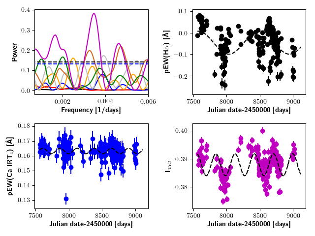
Figure 8: Same as in Fig. 5. GLS and time series for J20260+585 / Wolf 1069. In pEW(H$\alpha$), frequent flaring and the spacing of the observation leads to the period we found, while the same period may be present in the I_TiO data.

In an extended search, we also accepted periods shorter than one year but longer than 150 days (to avoid rotation periods). This led to an automatic detection of nine additional stars, which were all rejected by visual inspection. They are usually caused by the observing pattern or instead are weak quadratic trends. The only example of a star with a 0.7 a period, where the short period may be present in the TiO index alone, is the M5.0 star J20260+585 / Wolf 1069, which we show in the appendix in Fig. 8. Nevertheless, this GLS also shows a small peak in the window function that is caused by the observing scheme at about the period we found. We therefore also rejected this star by visual inspection.

All automatically found cycle candidates were inspected visually. This sometimes revealed that the period we found can also be explained by a quadratic or linear trend, especially when the period we found is near the length of the time baseline of the observations.

An example of an formerly unknown cycle candidate that fulfilled our automatic detection criteria and was not excluded by visual inspection is the M0.1 V star J22330+093/BD+08 4887, for which we show the GLS and time series in Fig. 5. While pEW(H$\alpha$) and pEW(Ca ii IRT) do show about the same period, the TiO index does not show the cycle period, but a shorter period is preferred. Since the broad peak in the GLS reveals that the period is not well constrained and no R${}^{\prime}_{\rm HK}$  data are available, the activity cycle period needs to be confirmed by photometry or other spectroscopic data.

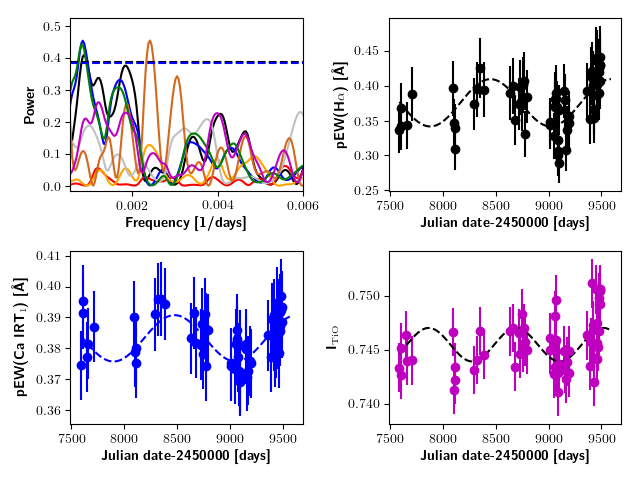
Figure 5: GLS and time series of J22330+093 / BD+08 4887. We show the GLS (left, top) with pEW(H$\alpha$) in black, pEW(Ca ii IRT₁) in blue, pEW(Ca ii IRT₂) in green, the TiO index in magenta, RV in yellow, dLw in grey, CRX in orange, and the window function in red. The dashed blue line indicates FAP=0.01 for the pEW(Ca ii IRT₁) data. Additionally, we show the time series for pEW(H$\alpha$) (right, top), for pEW(Ca ii IRT₁) (left, bottom), and the TiO index (right, bottom). The dashed black lines indicate the best sine fit for each indicator.

4 Results and discussion

With the methods described in the previous section, we found 26 automatic detections of long-term variability in our sample of 211 stars. Seven of these are linear trends, 14 are quadratic trends, and 12 are cycles (some stars exhibit more than one type of variability). From these numbers, we already excluded one linear trend, one quadratic trend, and one cycle, whose time series showed data gaps longer than 550 days and longer than 40% of the observation time baseline. Our results are summarised in Table 2, where we list the Karmn number of the star, a common name, the spectral type, the number of spectra we used, and the time baseline of the CARMENES observations. Furthermore, in the case of automatically found linear trends, we list the highest Pearson correlation coefficient (which does not necessarily correspond to the lowest or even a significant p-value), and in case of a quadratic trend, the number of flags that were triggered. In the case of significant GLS periods, we list the period length, and when available, the period length found in the R${}^{\prime}_{\rm HK}$ data. Additionally, we cite known literature values.

After the automatic detection, we inspected all variable time series by eye to determine the most appropriate detection in cases of multiple detections. For example, in all three cases when we rejected the linear trend, a quadratic trend was also found (twice by automatic detection, once by eye), and the quadratic trend was always preferred by visual evaluation. Six of the seven rejected cycles also showed a quadratic trend (four by automatic detection, two by visual inspection). Two of the stars with automatically detected quadratic trends (J04290+219 / BD+21 652, J05314-036 / HD 36395) also have a longer cycle detected in the R${}^{\prime}_{\rm HK}$  data, and the cycle length we found is about the length of the observation time baseline.

Finally, four linear trends, 11 quadratic trends, and five cycle periods passed the visual inspection. Therefore, 20 of our 26 automatically found long-term variable stars pass the visual inspection, which additionally leads to an appropriate categorisation. Since our adopted errors are relatively large, we refrained from applying an F-test and performed the sorting by eye. The stars that passed visual inspection are marked with an asterisk in Table 2, where we also list some remarks from the visual inspection for many stars.

Table 2: Proposed linear and quadratic trends and cycle periods for the stellar sample.

Karmn	Name	SpTa	No.	Time	Trendb	Para-	Cycle	R${}^{\prime}_{\rm HK}$ d	Visual	Literature
			of	baseline	corr-	bolicc	auto	cycle	inspectione	cycle
			spec.	[a]	coeff		[a]	[a]		[a]	[a]
J09144+526	HD 79211	M0.0	153	2.7	0.693	.	1.9	exist (13.2)	nc, pa (Ca+H$\alpha$)
J12123+544S	HD 238090	M0.0	104	3.3	…	9	1.5	…	nc, pa*
J13450+176	BD+18 2776	M0.0	29	6.0	$-$0.653	.	…	…	*
J14257+236W	BD+24 2733A	M0.0	63	3.5	0.829	10	1.2	…	nc, pa*
J02222+478	BD+47 612	M0.5	55	2.0	…	9	…	existg (14.0)	*	lin trend Rob13
J04290+219	BD+21 652	M0.5	167	2.1	…	10	1.8	3.4 (13.9)	nc, pa*
J06105$-$218	HD 42581 A	M0.5	49	3.9	…	9	2.7	14.3f (16.2)	cy*	8.4$\pm$0.3 SM16	8.3 DA19
J12312+086	BD+09 2636	M0.5	47	3.4	…	9	…	…	*
J13299+102	BD+11 2576	M0.5	354	6.1	…	.	1.5	0.7 (15.7)	nc, pa (Ca)
J05415+534	HD 233153	M1.0	95	4.1	0.705	.	1.4	…	lin*+cy*
J16581+257	BD+25 3173	M1.0	54	1.1	…	9	…	…	*
J18051$-$030	HD 165222	M1.0	51	2.5	…	9	…	7.6 (12.3)
J22330+093	BD+08 4887	M1.0	64	5.2	…	.	3.1	…	*
J23245+578	BD+57 2735	M1.0	61	4.6	$-$0.740	.	…	…	*
J02123+035	BD+02 348	M1.5	65	4.3	…	9	…	15.5f (16.0)	*
J03181+382	HD 275122	M1.5	56	4.9	$-$0.770	10	…	…	pa*
J05314$-$036	HD 36395	M1.5	90	2.2	…	9	1.9	11.6f (16.3)	nc, pa*	10.8/ 3.9 SM16	3.5 K19
J16254+543	GJ 625	M1.5	30	1.3	…	9	…	…	*	3.3$\pm$1.5 SM18
J22057+656	G 264-018 A	M1.5	90	2.6	…	10	…	…	*
J22565+165	HD 216899	M1.5	548	6.1	…	.	5.4	15.5f (16.2)		15.5 Per21
J11110+304W	HD 97101 B	M2.0	51	4.1	…	9	…	10.1 (13.2)	*
J01518+644	G 244-037	M2.5	21	5.2	0.705	.	…	…	*
J19169+051N	V1428 Aql	M2.5	125	1.7	…	10	…	12.6f (14.3)		3.3$\pm$0.4 DA19	9.3$\pm$1.9 SM16
J16167+672N	EW Dra	M3.0	103	4.5	…	9	…	…	*
J07274+052	Luyten’s Star	M3.5	734	6.1	…	.	2.8	2.8f (14.8)	*	6.6$\pm$1.3 SM16	2.8 Per21
J18346+401	LP 229-017	M3.5	77	4.8	…	.	4.0	…	*

AK17: Alekseev & Kozhevnikova (2017); DA19: Díez Alonso et al. (2019); Per21: Perdelwitz et al. (2021); Rob13: Robertson et al. (2013); SM16: Suárez Mascareño et al. (2016); SM18: Suárez Mascareño et al. (2018).
^a Spectral (sub-)type of M
^b Pearson’s $r$
^c Number of flags triggered in the parabolic trend search
^d Given in parentheses is the observation time baseline for the R${}^{\prime}_{\rm HK}$  measurements
^e Abbreviations: nc: no cycle, pa: parabolic trend, lin: linear trend, *:Confirmed by visual inspection.
^f Automatic detection of the period based on R${}^{\prime}_{\rm HK}$  data alone, see Sect. 4.4.
^g exist: R${}^{\prime}_{\rm HK}$   data exist, but the criterion of FAP$<0.001$ in the GLS is not met.

4.1 Comparison to literature

For seven of the stars showing systematic variability, we could find published cycle lengths. Unfortunately, the situation is complicated and we find only few agreements. For J02222+478 / BD+47 612, we find a quadratic trend that agrees with the linear trend found by Robertson et al. (2013). The same is true for J16254+543 / GJ 625, where we find a quadratic trend that agrees with the cycle period found by Suárez Mascareño et al. (2018). For J05314-036 / HD 36395, a long and a short cycle is known. Since the time baseline of the CARMENES data is about 1.5 a shorter than the shorter cycle, the quadratic trend agrees with this short cycle, while the period found in the R${}^{\prime}_{\rm HK}$  data agrees with the long cycle.

For J19169+051N / V 1428 Aql, a short and a long cycle are known from photometry. As the observation time baseline of the CARMENES data is rather short for this star, we find a quadratic trend, while in the R${}^{\prime}_{\rm HK}$  data, we find a period that roughly agees with the longer literature period. For J22565+165 / HD 216899, we find a period of 5.4 a without visual confirmation that is much shorter than the period found in the R${}^{\prime}_{\rm HK}$  data. J06105-218 / HD 42581 A and J07274+052 / Luyten’s star are discussed in Sect. 4.2 because we found a visually convincing cycle period.

4.2 Promising activity cycle candidates

In the following, we discuss the five starst that are the most promising candidates for activity cycles for which more than a full cycle is covered by the CARMENES observations and that passed the visual inspection. The first of these stars is J22330+093 / BD+08 4887. This star was discussed in Sect. 3.3, see Fig. 5.

In the M1.0 dwarf J05415+534 / HD 233153 a rather short period of only 1.4 a was found that we show in the left panel of Fig. 6 in H$\alpha$ and Ca ii IRT₁. The trend that was also detected automatically is overlaid. It may indicate two different cycle periods. However, the TiO index does not show any variation, not even the trend.

For the M3.5 V star J18346+401 / LP 229-017, we show the GLS and time series in the right panel of Fig. 6. Although the period has about the same length as the observation time baseline, we opted for the cycle and not for a quadratic trend by visial inspection in this special case. The period can be seen quite clearly in H$\alpha$ and Ca ii IRT, but not in TiO, where a shorter period is found.

The case for the M0.5 dwarf J06105-218 / HD 42581 A is slightly more complicated. A cycle of about 8.3 a is known from the literature (Suárez Mascareño et al., 2016; Díez Alonso et al., 2019). In the R${}^{\prime}_{\rm HK}$  data, we find a peak at about twice this period, which may be a sub-harmonic because there is also a (non-significant) peak at 7.9 a, which would agree with the literature value. In the CARMENES data, we also find a cycle of 2.7 a length, which is visually confirmed. Either this is a quasi-periodic episode, or this is a second, shorter cycle. We show the data of this star in Fig. 9.

For the M3.5 dwarf J07274+052 / Luyten’s star, we find a period of 2.8 a, in agreement with the findings from the R${}^{\prime}_{\rm HK}$  data, which has been published previously (Perdelwitz et al., 2021). There is a second published period of 6.6$\pm$1.3 a (Suárez Mascareño et al., 2016) that may be about twice the shorter cycle. A second significant peak lies at 6.1 a in the GLS of the R${}^{\prime}_{\rm HK}$  data. The correct period cannot be decided from the available data, which are shown in Fig. 10.

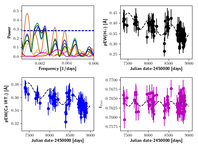
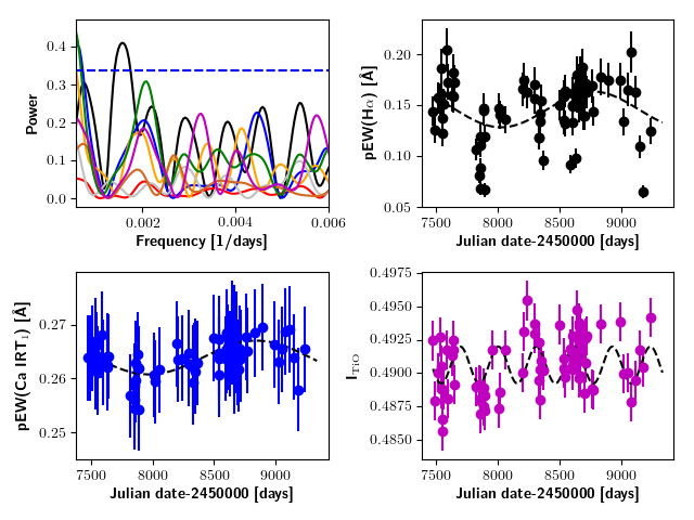
Figure 6: Same as in Fig. 5. GLS and time series of J05415+534 / HD 233153 (left) and J18346+401 / LP 229-017 (right). We note that for J05415+534 / HD 233153, a linear trend was found as well, which we include in the sine fit for pEW(H$\alpha$) and pEW(Ca ii IRT₁). We further note that for J18346+401 / LP 229-017, the highest peak of pEW(H$\alpha$) in the GLS is at about twice the frequency as for the other chromospheric indicators that triggered the cycle detection. We therefore used half the frequency for the sine fit of pEW(H$\alpha$) as well.

4.3 Known cycles without detected long-term variation in the chromospheric indicators

We fail to find systematic long-term activity variations with our automatic search algorithms for 34 stars with proposed cycles from the literature. These non-detections fall into three categories: First, the star was excluded from our data analysis due to binarity (1 star) or fewer than 20 observations (4 stars); or it showed possibly problematic long data gaps (1 stars). Second, visual inspections revealed indications of linear or quadratic trends or even cycles (18 stars) in individual chromospheric indicators. Third, we do not find any systematic long-term variations (10 stars). We list all these stars in Table 3 and also remark on the visual inspection of the CARMENES data.

An example that demonstrates the difficulties well is the star J06371+175 / HD260655. We were able to visually identify a linear trend in the pEW(Ca ii IRT) time series, while we find a quadratic trend in pEW(H$\alpha$) and I_TiO. Since the baseline of the CARMENES observations is 6.1 a, this neither agrees with the 7.3 a cycle from the R${}^{\prime}_{\rm HK}$   data nor with literature values of 2-3 a from Díez Alonso et al. (2019) or 4.9 a from Suárez Mascareño et al. (2016). Since the trend we found in the data indicates a cycle that is longer than 10 years, the star may exhibit multiple cycles. We caution, however, that the two cycle length values from the literature (both photometry) also disagree, and claims of more than two cycles per star would remain highly speculative given the available data. Alternatively, this may indicate quasi-periodic episodes or changes in the cycle length, such as those known from the Sun.

Another instructive example is the star J06548+332 / Wolf 294/GJ 251. Stock et al. (2020) found a significant 600 d cycle in RV data using HIRES data alone, while the signal is not present in their CARMENES RV data. Their inspection of chromospheric indicators reveals a 660 d cycle in the H$\alpha$ indicator and a 300 d cycle length in CRX and Na i D. While we find a significant peak at about 630 d in the TiO index and pEW(Ca ii IRT₂), the GLS of the pEW(H$\alpha$) shows an even higher peak at about 1680 d (including newer data), while the R${}^{\prime}_{\rm HK}$  data favour about twice that period with a 3300 d period, which may indicate that the period in pEW(H$\alpha$) is a harmonic, the longer period of which cannot be found because the observation time baseline is too short. Further investigation is required to determine whether there are indeed a short (600 d=1.6 a) and a long cycle (9 a).

The star J11033+359 / Lalande 21185 is a peculiar case, for which we find a visually convincing period in H$\alpha,$ but not in any other chromospheric indicator. This period was also reported with a similar length by Stock et al. (2020) for their (shorter time baseline) CARMENES data alone. However, they replaced that period for a period that was more than twice longer based on their combined CARMENES and SOPHIE data analysis. This value in turn ais bout half the value we found from the R${}^{\prime}_{\rm HK}$  data.

On the other hand, there are examples such as J07446+035 / YZ CMi, J10196+198 / AD Leo, J17303+055 / BD+05 3409, J20525$-$169 / LP816-060, or J22096$-$046 / BD$-$05 5715, where we find a linear or quadratic trend that agrees well with the cycles proposed in literature by visual inspection in single activity indicators. Moreover, the star J18580+059 /BD+05 3993 was discussed in detail by Suárez Mascareño et al. (2018). Our observation started just after the time baseline discussed by them, but a downward trend was expected to occur afterwards, which is what we observe, but only by visual inspection.

Although the existence of multiple cycles in a single star may explain some of the discrepancies we found, the star may also undergo phases of quasi-systematic episodes and therefore show a different behaviour at different times. Another problem is that different activity indicators reveal different behaviour. Trends or periods are often only found in one activity indicator, while the others show a constant, chaotic, or even contradicting systematic behaviour. While the first two possibilities can be explained by the different sensitivity of the indicators, the latter is not expected. It may indicate time lags between the indicators in the (quasi-)systematic development. Possible examples for different sensitivity are the stars J08161+013 / GJ 2066 and J11033+359 / Lalande 21185, for which we find a quadratic trend or even a cycle in a single activity indicator, while the others are rather constant. An example in which activity indicators show a different behaviour is J06548+332/Wolf 294 (discussed above, linear trend in pEW(Ca ii IRT), quadratic trend in pEW(H$\alpha$)). Since the discrepancy is seen only in the last observing block, this indicates a time lag between the indicators.

Another problem may be imposed by the observation scheme. An example is J08298+297 / DX Cnc, for which the observation pattern shows some tight blocks with larger gaps in between. Together with the rather high activity level of J08298+297 / DX Cnc, this may be the cause for our finding only insignificant peaks in the GLS at about the known cycle period in pEW(H$\alpha$) and pEW(Ca ii IRT).

Table 3: Cycles from the literature where no long term variation was found by the automatic search.

Karmn	Name	SpTa	No. of	Time	R${}^{\prime}_{\rm HK}$	Visual	Literature
			spectra	baseline	cycle	inspection	cycle
				[a]	[a]		[a]	[a]	[a]
J06371+175	HD 260655	M0.0	115	6.1	7.3c (13.7)	lin(Ca), pa(H$\alpha$,TiO);R${}^{\prime}_{\rm HK}$  2nd peak at 14.5 a	2-3 DA19	4.9$\pm$0.4 SM16
J19346+045	BD+04 4157	M0.0	53	3.2	…		3.0$\pm$0.8 DA19
J17303+055	BD+05 3409	M0.0	53	2.5	11.9c (12.3)	pa (H$\alpha$+Ca)	11.9 Per21
J18353+457	BD+45 2743	M0.5	16	1.2	…	too few data	2.3$\pm$0.5 SM18
J18580+059	BD+05 3993	M0.5	32	1.3	exist (10.8)	lin(H$\alpha$+Ca)	5.6$\pm$0.1 SM18
J20451$-$313	AU Mic	M0.5	90	1.3	…		4.8,2.8 K19	40.6 BK20
J22021+014	BD+00 4810	M0.5	75	3.1	exist (14.3)	lin	8.5$\pm$1.1 SM16
J00051+457	GJ 2	M1.0	52	1.9	exist (14.0)		3.2$\pm$0.1 SM18
J00183+440	GX And	M1.0	213	4.1	exist (14.1)	weak pa(H$\alpha$, TiO)	2.8$\pm$0.5 SM18
J07361$-$031	BD-02 2198	M1.0	45	6.0	…	known binary (Ba21)	11.5$\pm$1.9 DA19
J22559+178	StKM 1-2065	M1.0	11	1.4	…	too few data	2-3 DA19	4.4$\pm$0.9 SM18
J10122$-$037	AN Sex	M1.5	74	2.2	2.6 (16.2)		3.2 $\pm$0.4 DA19	13.6$\pm$1.7 SM16
J11033+359	Lalande 21185	M1.5	376	4.9	13.2c (14.9)	3.2a cycle (H$\alpha$)	7.9 SN20
J13457+148	HD 119850	M1.5	249	2.2	exist (17.5)		9.9$\pm$2.8 SM16
J15218+209	OT Ser	M1.5	52	2.8	7.3c (9.3)		6.5$\pm$0.8 DA19
J04429+189	HD 285968	M2.0	23	1.0	7.3c (13.8)	weak lin trend	5.9$\pm$0.7 SM16	5.6 GdS12
J08161+013	GJ 2066	M2.0	70	5.0	7.4 (11.3)	pa(Ca)	4.1$\pm$0.7 DA19
J11000+228	Ross 104	M2.5	55	2.2	0.7 (8.1)	lin (TiO)	5.3$\pm$0.6 SM16
J12350+098	GJ 476	M2.5	9	4.8	…	too few data	2.9 Rob13
J06548+332	Wolf 294	M3.0	342	6.1	9.0 (14.0)	4.5 a cycle (H$\alpha$)	1.6 SN20
J10196+198	AD Leo	M3.0	44	1.9	…	data gap; lin	27 AK17	7.6 Buc14
J15194$-$077	HO Lib	M3.0	52	3.5	4.0c (10.7)	lin (TiO)	4.5 K19/Rob13	6.2$\pm$0.9 SM16	3.85 GdS12
J08409$-$234	LP 844-008	M3.5	28	4.2	exist (13.0)	lin (TiO+Ca), pa (H$\alpha$)	5.2$\pm$0.3 SM16
J13427+332	Ross1015	M3.5	19	4.0	…	too few data	quadr trend Rob13
J16303$-$126	V2306 Oph	M3.5	88	3.5	4.2c (11.2)	pa(H$\alpha$)	3.9$\pm$1.0 DA19	4.4$\pm$0.2 SM16
J22096$-$046	BD-05 5715	M3.5	59	3.4	exist (15.0)	pa (H$\alpha$+TiO)	10.2$\pm$0.9 SM16
J18498$-$238	V1216 Sgr	M3.5	51	1.0	exist (13.3)		4.9 K19	7.1$\pm$0.1/2.1$\pm$0.1 SM16	4.1/1.0 IB21
J11477+008	FI Vir	M4.0	51	3.0	exist (14.2)	pa (TiO)	4.5$\pm$2.0 DA19	4.1$\pm$0.3 SM16
J20525$-$169	LP 816-060	M4.0	35	4.4	…	pa (H$\alpha$+Ca)	10.6$\pm$1.7 SM16
J22532$-$142	IL Aqr	M4.0	67	3.5	exist (14.8)		4.5$\pm$0.7 DA19
J07446+035	YZ CMi	M4.5	48	2.0	…	weak lin trend (H$\alpha$+Ca)	10.6$\pm$1.7 SM16
J08413+594	LP 090-018	M5.5	51	3.9	…		14 LS20
J10564+070	CN Leo	M6.0	66	2.2	…		8.9$\pm$0.2 SM16
J08298+267	DX Cnc	M6.5	29	4.8	…	lin(TiO), 2.5a cycle insignificant (H$\alpha$,Ca)	2.67 BK20

Ba21: Baroch et al. (2021); BK20: Bondar’ & Katsova (2020); Buc14: Buccino et al. (2014); DA19: Díez Alonso et al. (2019); GdS12: Gomes da Silva et al. (2012);
IB21: Ibañez Bustos et al. (2021); K19: Küker et al. (2019); LS20: Lopez-Santiago et al. (2020) Per21: Perdelwitz et al. (2021); Rob13: Robertson et al. (2013);
SM16: Suárez Mascareño et al. (2016); SM18: Suárez Mascareño et al. (2018); SN20: Stock et al. (2020).
^a Spectral (sub-)type of M
^b Given in parentheses is the observation time baseline for the R${}^{\prime}_{\rm HK}$  measurements
^c Automatic detection of the period based on R${}^{\prime}_{\rm HK}$  data alone, see Sect. 4.4.

4.4 Promising cycle candidates from R${}^{\prime}_{\rm HK}$  alone

Since the R${}^{\prime}_{\rm HK}$  data usually show a much longer observation time baseline and R${}^{\prime}_{\rm HK}$  is known to be suitable for activity cycle search in more solar-type stars (Baliunas et al., 1995; Brandenburg et al., 2017), we decided to perform an additional search on the R${}^{\prime}_{\rm HK}$  data alone. This can be achieved even though the data originate from seven different telescopes, because instrument offsets were minimised by extracting the R${}^{\prime}_{\rm HK}$  values using a direct comparison to model spectra (for further discussion, see Perdelwitz et al. (2021)). Since only a single chromospheric indicator was used this time and a cross-check with other indicators is therefore missing, we opted in this search for a much better FAP $<0.0005$ and excluded all stars with fewer than 20 spectra or automatically detected periods shorter than one year. Since the R${}^{\prime}_{\rm HK}$  data often have a much coarser sampling, we also excluded stars with data gaps longer than a quarter of the observation time baseline and longer than 1000 days.

We repeated the GLS analysis and found that 22 cycle candidates fulfilled these criteria. Out of these, 7 correspond to stars that also show a variability detection in the CARMENES data and are therefore listed in Table 2. Another 6 correspond to stars with a proposed cycle from the literature and are therefore listed in Table 3. A cycle period detection based on the R${}^{\prime}_{\rm HK}$  data alone is indicated in both of the tables. The remaining 9 cycle candidates are detections based on R${}^{\prime}_{\rm HK}$  alone, and none of these was rejected by visual inspection. We list them in Table 4 with their spectral type, number of observations, the R${}^{\prime}_{\rm HK}$  observation time baseline, and remarks on the visual inspection of the CARMENES data. We show the GLS and time series of R${}^{\prime}_{\rm HK}$  of the most promising 6 candidates in the appendix in Figs. 11, 12, and 13.

This better performance of the R${}^{\prime}_{\rm HK}$  data in the cycle search is partly caused by the longer time baseline, which allows us to find cycles that are not yet covered by the CARMENES data. We therefore state the CARMENES baselines in Table 4, where appropriate. Nevertheless, in some of these cases, no trends are found, either. While the reason may be that the CARMENES observations incidentally cover the maximum or minimum of the cycle, the different sensitivity of the lines may also play a role. We discuss this in Sect. 4.6 and reveal that the relative amplitude in R${}^{\prime}_{\rm HK}$  data is higher than of the other line pEWs.

Table 4: Proposed cycle periods using R${}^{\prime}_{\rm HK}$  alone for stars without CARMENES data detections or literature values.

Karmn	Name	SpTa	No.	Time	R${}^{\prime}_{\rm HK}$	Visual
			of	baseline	cycle	inspection
			spec.	[a]	[a]
J10251$-$102	BD-09 3070	M1.0	62	9.0	2.3	6.1 a CARMENES baseline, weak trend in Ca, H$\alpha$
J11054+435	BD+44 2051A	M1.0	125	8.1	1.8	data gap, 2.7 a in Ca, H$\alpha$b
J14010$-$026	HD 122303	M1.0	226	11.7	2.6	1.3 a CARMENES baseline, no trend
J20533+621	HD 199305	M1.0	73	14.1	7.8	3.8 a CARMENES baseline, 3.2 a in H$\alpha$b
J23492+024	BR Psc	M1.0	207	14.2	27.3	5.6 a CARMENES baseline, maybe trend in H$\alpha$
J20450+444	BD+44 3567	M1.5	80	6.7	7.2	3.7 a in Ca, H$\alpha$b
J10289+008	BD+01 2447	M2.0	204	12.9	3.3	3.1 a in Ca, H$\alpha$b
J14294+155	Ross 130	M2.0	52	7.7	1.9	too few CARMENES data
J11421+267	Ross 905	M2.5	302	15.2	17.2	2.3 a CARMENES baseline, no trend

^a Spectral (sub-)type of M
^bperiods given correspond to the highest peak in the periodogram, regardless of the assigned FAP.

4.5 Dependence on spectral type

To identify a possible dependence on spectral sub-type, we show in Fig. 7 the number of stars and the number of automatic long-term variability detections (including the nine detections based on R${}^{\prime}_{\rm HK}$  alone). The percentage of systematically variable stars drops toward later spectral types from about 15-30% in early-M dwarf stars to lower than 5% for mid-M dwarfs. We do not find any sign of a systematic long-term variability for any star with spectral type later than M4.0 V. This cannot be caused by observational biases because the mean observation time baseline of the included M4 stars is even longer than for M0 stars. Although the mean number of observations for M4 stars is somewhat lower than for M0 stars, the number of stars with more than 50 usable observations is higher for M4 stars than for M0 stars. Noise should not play a role here either because we excluded spectra with a too low level of the signal-to-noise ratio, and this is usually only an issue for stars with spectral type M5 and later because the exposure time never exceeds 1800 s. Either these latest type, fully convective stars do not have activity cycles, or they may not found due to frequent flaring.

Flaring was also identified as the main reason for variability in fully convective M dwarfs in a study by Medina et al. (2022), who found only for one very young star a correlation of the EW(H$\alpha$) to the rotational phase in a sample of 13 stars. The short timescales of steallar variability in their study, which was observed with high cadence, suggest an origin of the variability in flares. Although we excluded large flares, frequent low-level flaring would lead to a broadening of the distribution of the individual indicators and would thus not be handled by $\sigma$ clipping. This can lead to a veiling of possible activity cycles.

The stars with cycle values proposed in the literature also include stars with spectral type M4 and later. We therefore note that all these stellar cycles have been detected by photometry and not by chromospheric indicators. At least for J07446+035 / YZ CMi and J20525-169 / LP 816-060, visual inspection also revealed weak linear or parabolic trends in these stars, while for J08298+297 / DX Cnc, we find an insignificant period of the cycle length from the literature. This may indicate that in these relatively late-M dwarfs, the sensitivity of the chromospheric indicators to cyclic activity is lower than in early-type M dwarfs. Next to flaring, this may be caused by generally high chromospheric filling factors, for example, which would lead to low amplitudes in the cycle modulation and might therefore hamper the detection of a cycle.

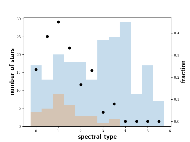
Figure 7: Number of stars per spectral sub-type (blue bars, left y-axis), and number of stars with an automatic variability detection (red bars, left y-axis). We show the fraction of stars with variability per spectral sub-type as black dots corresponding to the right y-axis.

4.6 Sensitivity of the different indicators

We analysed the chromospheric indicator that was most often involved in the trend or cycle detection for the different search methods. For the linear trend search, the Ca ii IRT lines, H$\alpha,$ and dLw most often led to a trend with between 5 and 7 detections each, while the TiO index and CRX led to one detection, and RV to zero detection. For the parabolic search, we find that pEW(H$\alpha$), pEW(Ca ii IRT), and I_TiO  each were triggered for all detected stars. Finally, for the cycle search, again the Ca ii IRT lines were involved most often in a cycle detection (12 detections each), followed by H$\alpha$ with 8 detections, dLw with 6 detections, TiO and CRX with 4 detections, and RV with 3 detections. We conclude that long-term variability is most easily found in the Ca ii IRT lines, followed by H$\alpha$ and dLw, while TiO, RV, and CRX are less well suited.

For a better comparison, we also considered the amplitudes of the different indicators. We computed the amplitude as the relative difference of the median of the ten highest and ten lowest data points in the time series with a detected (linear or quadratic) trend or period (regardless of whether the indicator triggered the detection). For the time series showing a trend, the amplitude is only a lower threshold. This leads to median amplitudes of 14% for pEW(H$\alpha$), of 4% for pEW(Ca ii IRT), and of 0.08% for I_TiO. This underlines the higher sensitivity of H$\alpha$ compared to Ca ii IRT and especially I_TiO. The highest sensitivity is found for R${}^{\prime}_{\rm HK}$ , with a relative median amplitude of 46%. The relatively low amplitudes of pEW(Ca ii IRT) come as a surprise because Ca ii IRT triggered the most automatic detections. This better performance compared to pEW(H$\alpha$) may be caused by a larger influence of flares on the pEW(H$\alpha$), because the line is formed at larger heights in the chromosphere than Ca ii IRT.

4.7 Comparison of cycles to rotation periods

While Böhm-Vitense (2007) found two distinct relations between rotation period and cycle length for active and inactive G and K stars, Küker et al. (2019) found virtually no dependence of the cycle length on rotation period for early-M dwarfs. They found two groups with characteristic cycle times, however, first the fast rotators with rotation periods shorter than one day and cycle lengths of about one year, and second, stars with longer rotation periods and a cycle length between three to five years. Moreover, Suárez Mascareño et al. (2016) did not find a correlation between rotation period and cycle length for the M dwarfs included in their study. Nevertheless, they find a weak correlation for earlier-type stars. Suárez Mascareño et al. (2018) found a weak correlation of rotation period with cycle length for M dwarfs using literature values in addition to their measurements, but also stated that a correlation test showed that there is a 37% probability of the correlation being spurious.

Although we have 25 stars with known rotation periods shorter than one day in our sample, these stars are all of spectral type M3.5 or later, and no long-term variation is found for any of these stars. If the finding of Küker et al. (2019) is correct that such short cycles are found only for fast rotators, our visual evaluation that none of the found periods shorter than one year is also consistent because none of these stars is a fast rotators.

We searched for a correlation of rotation period $P_{\mathrm{rot}}$ and cycle length $P_{\mathrm{cyc}}$ using our cycle detections from CARMENES and R${}^{\prime}_{\rm HK}$  data and all literature values from Table 3. This resulted in 34 stars (13 from our own measurements and 21 from the literature) for which rotation periods are also available. We performed an analysis similar to that of Suárez Mascareño et al. (2018) and computed the slope of $\log(P_{\mathrm{cyc}}/P_{\mathrm{rot}})$ versus $\log(1/P_{\mathrm{rot}})$ , which gives $1.1\pm 0.1$ and therefore does not deviate significantly from 1.0. This implies that there is no correlation between rotation period and cycle length.

5 Conclusions

We searched in a sample of 211 M dwarfs for long-term systematic variability in chromospheric indicators. The observations were taken from the more than 19 000 CARMENES observations, considering only stars with more than 19 observations and an observation time baseline of more than 200 days. We not only considered the pEW of H$\alpha$ and the Ca ii IRT  lines as chromospheric indicators, but also more recently defined activity indicators: the TiO-index, RV, CRX, and dLw. In a sub-sample of 186 stars, we also used already published R${}^{\prime}_{\rm HK}$ data with much longer observation time baselines, originating from different instruments. In these we performed an automatic search for periods and other long-term systematics, namely linear trends and quadratic trends. The automatic search led to 26 detections of this systematic long-term variability. By visual inspection, we rejected 6 of these detections and sorted the remaining stars uniquely into our different variability categories, leaving us with four linear trends, 11 quadratic trends, and five periods. We show all the five stars with proposed periods in the Figs. 5, 6, 9, and 10. Analysing the R${}^{\prime}_{\rm HK}$  data alone and applying a stricter FAP threshold than for the combined data set, we found an additional nine promising cycle candidates, which are shown in Figs. 11, 12, and 13. Furthermore, we found that from the analysed indicators that are available from the CARMENES observations, the pEWs of Ca ii IRT and H$\alpha$ lines are best suited for a study of long-term variability. Comparison of the relative median amplitudes of the systematic variation shows that R${}^{\prime}_{\rm HK}$  has the highest amplitude, followed by pEW(H$\alpha$), pEW(Ca ii IRT), and I_TiO. Therefore, we propose that future activity cycle searches performed in chromospheric indicators should concentrate on R${}^{\prime}_{\rm HK}$ , pEW(H$\alpha$), or pEW(Ca ii IRT). On the other hand, we were unable to confirm many cycles proposed in the literature on the basis of photometric data, especially for later-type stars, which may suggest that photometry is even better suited for an activity cycle search than chromospheric indicators in these stars. Most important for RV exoplanet searches, we found that RV variations are not a sensitive indicator of systematic long-term chromospheric variability in our study.

The detection rate of systematic long-term variability in all our sample stars is about 12% from the CARMENES data alone. This is low in comparison to Suárez Mascareño et al. (2018), for instance, who found cycles in about 18% of their M0–M3 stars using chromospheric indicators as well. When we only consider our M0–M3 stars, we have an even slightly higher detection rate of about 25%, which is to be expected because we additionally searched for linear and quadratic trends. The detection rate of the long-term variability dramatically decreases along the M spectral sequence to later-type stars. For stars M4.0 and later, we do not find any activity cycle. These fully convective stars may either exhibit no cycles caused by the different dynamo underlying their activity phenomena, or the existence of cycles is veiled in the chromospheric indicators by frequent flaring. This latter possibility is underlined by the study of Suárez Mascareño et al. (2016), who found cycles in about 50% of their M dwarfs for fully convective stars as well, using photometry. Again, this suggests that photometry is better suited for cycle searches in M dwarfs.

Although the CARMENES observation span little more than six years at most, we found some short-cycle candidates in agreement with literature values, or promising parts of cycles where sometimes longer (mostly photometrically determined) cycles were already known. We also identified a few cases for which modulation periods reported in the literature could not be confirmed. The most promising linear and quadratic trends stress that the observations need to be continued in the future to accumulate data that cover at least a whole cycle or reveal the current data to be a quasi-systematic episode.

Appendix A Further examples of long-term variability

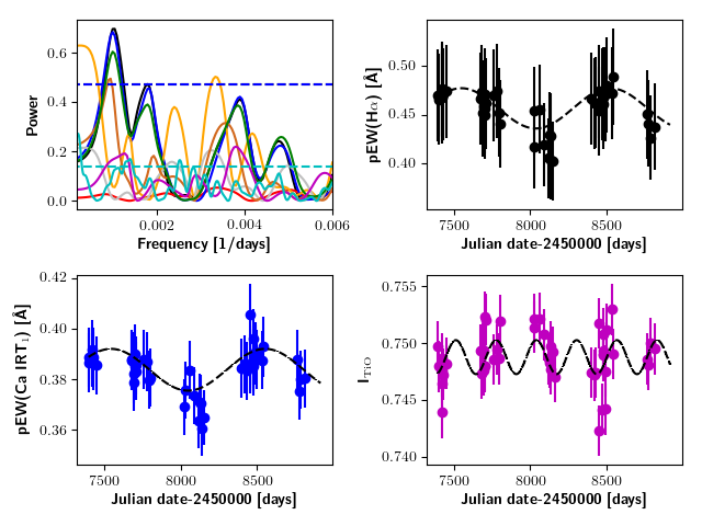
Figure 9: Same as in Fig. 5, but for J06105$-$218 / HD 42581 A.

Figure 10: Same as in Fig. 5, but for J07274+052 / Luyten’s star. We omit the error bars for clarity.

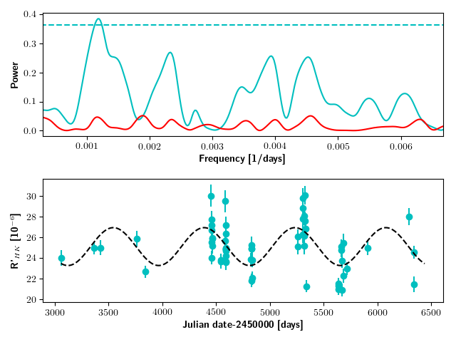
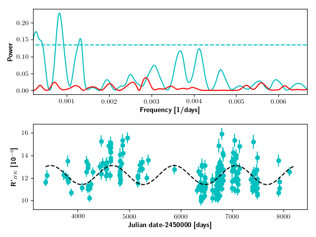
Figure 11: GLS and time series of J10251$-$102 / BD$-$09 3070 (M1.0 V, left) and J10289+008 / BD+01 2447 (M2.0 V, right). In the GLS (top), we show the power of the R${}^{\prime}_{\rm HK}$  data in cyan, the dashed cyan line marks the 0.0005 FAP level, and the red line is the power of the window function. In the time series (bottom), we show the R${}^{\prime}_{\rm HK}$  values as cyan dots and the best-fit sine function as the dashed black line.

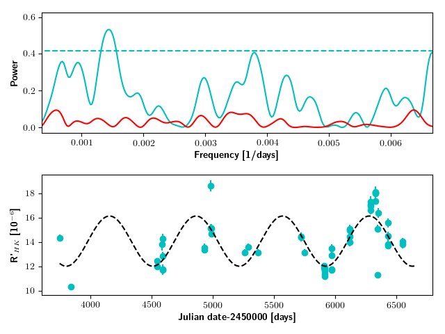
Figure 12: Same as Fig. 11, but for J11421+267 / Ross 905 (M2.5 V, left) and J14294+155 / Ross130 (M2.0 V, right).

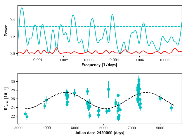
Figure 13: Same as Fig. 11, but for J20450+444 / BD+44 3567 (M1.5 V, left) and J20533+621 / HD 199305 (M1.0 V, right).