Metric Elicitation; Moving from Theory to Practice

Abstract

Metric Elicitation (ME) is a framework for eliciting classification metrics that better align with implicit user preferences based on the task and context. The existing ME strategy so far is based on the assumption that users can most easily provide preference feedback over classifier statistics such as confusion matrices. This work examines ME, by providing a first ever implementation of the ME strategy. Specifically, we create a web-based ME interface and conduct a user study that elicits users’ preferred metrics in a binary classification setting. We discuss the study findings and present guidelines for future research in this direction.

1 Introduction

Given a classification task, which performance metric should the classifier optimize? This question is often faced by practitioners while developing machine learning solutions. For example, consider cancer diagnosis where a doctor applies a cost-sensitive predictive model to classify patients into cancer categories [12]. Although it is clear that the chosen costs directly determine the model decisions, it is not clear how to quantify the expert’s intuition into precise quantitative cost trade-offs, i.e., the performance metric [1, 13].

Hiranandani et al. [3, 4] addressed this issue by formalizing the Metric Elicitation (ME) framework, whose goal is to estimate a performance metric using user feedback over confusion matrices. The motivation is that by employing metrics that reflect a user’s innate trade-offs given the task, context, and population at hand, one can learn models that best capture the user preferences [3]. As humans are often inaccurate in providing absolute quality feedback [10], Hiranandani et al. [3] propose to use pairwise comparison queries, where the user (oracle) is asked to provide a relative preference over two confusion matrices. Figure 1 (reproduced from [3]) depicts the ME framework.

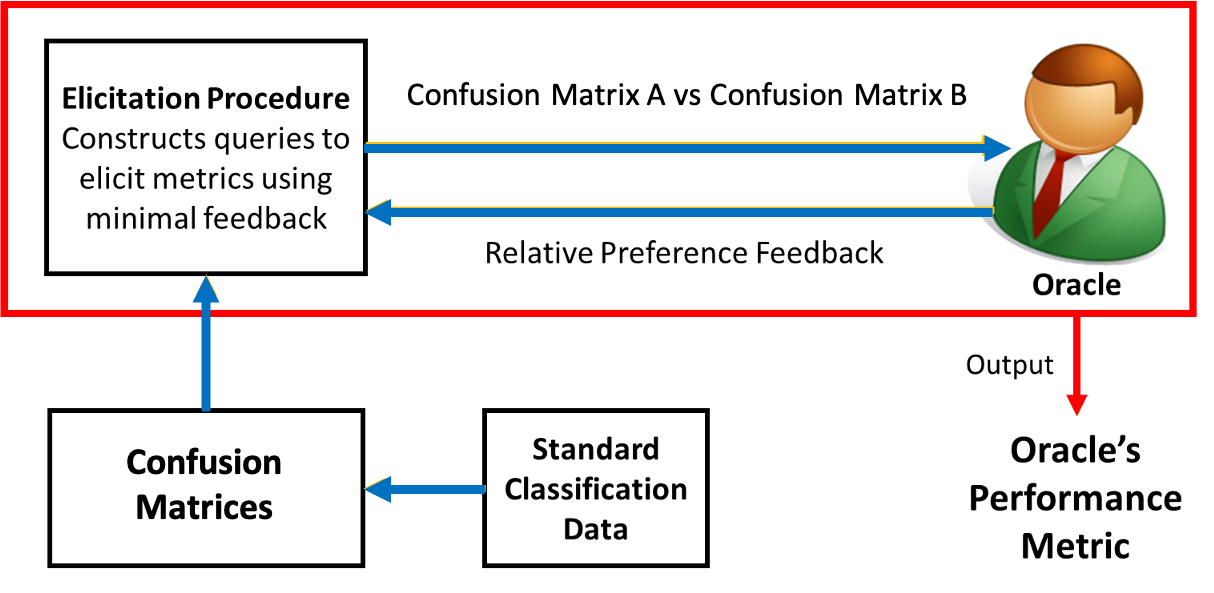
Figure 1: Metric Elicitation framework [3].

Prior literature on ME has proposed elicitation strategies for binary [3], multiclass [4], and multiclass-multigroup [6, 5] classification settings, which assume the presence of an oracle that provides relative preference feedback over confusion matrices. However, to our knowledge, there are no reported implementations testing the ME framework and the assumption that users can effectively report confusion matrix comparisons. In this paper, we bring theory closer to practice by providing a first ever practical implementation of the ME framework and its evaluation. Our contributions are summarized as follows:

• We propose a visualization for pairwise comparison of confusion matrices that adapts the visualization of individual confusion matrices from Shen et al. [11].

• We then integrate the visualization within a web User Interface (UI) that asks for relative preference feedback over confusion matrices. Furthermore, the UI implements Algorithm 1 from Hiranandani et al. [3] and uses real-time responses from the subjects to elicit their performance metrics.

• Using the proposed UI, we perform a user study with ten subjects and elicit their linear performance metrics for a cost-sensitive binary classification setting. We evaluate the quality of the recovered metrics and also conduct post-task, think-aloud-style interviews with the subjects.

• Lastly, we present guidelines for practical implementation of the ME framework for future research.

2 Problem Setup and Background

Let $X\in{\cal X}$ and $Y\in\{0,1\}$ represent the input and output random variables respectively (0 = negative class, 1 = positive class), and let $\pi=\mathbb{P}(Y=1)$ denote the probability of the positive class. We denote a classifier by $h$. A confusion matrix for a classifier $h$ comprises true positives $(TP(h)\mathrel{\mathop{\ordinarycolon}}=\mathbb{P}(Y=1,h=1))$, false positives $(FP(h)\mathrel{\mathop{\ordinarycolon}}=\mathbb{P}(Y=0,h=1))$, false negatives $(FN(h)\mathrel{\mathop{\ordinarycolon}}=\mathbb{P}(Y=1,h=0))$, and true negatives $(TN(h)\mathrel{\mathop{\ordinarycolon}}=\mathbb{P}(Y=0,h=0))$. The components of the confusion matrix can be decomposed as: $FN(h)=\pi-TP(h)$ and $FP(h)=1-\pi-TN(h)$, which reduces the four dimensional space to two dimensional space, and thus we interchangeably refer to the confusion matrix as confusion vector and denote it by $\mathbf{c}(h)=(TP(h),TN(h))$.

In this work, we seek to elicit a linear performance metric, which for some weights $\mathbf{a}$ is defined as: $\phi((TP(h),TN(h)))=a_{0}TN(h)+a_{1}TP(h).$ Since the metrics are scale invariant [9], we assume $\|\mathbf{a}\|_{1}=1$. Hence, the linear metrics can be defined using just one parameter as follows:

$$\phi((TP(h),TN(h)))\coloneqq a_{0}TN(h)+(1-a_{0})TP(h),\quad\text{where}\quad a_{0}\in[0,1].$$ (1)

One example of linear metrics is weighted-accuracy [7]. Specifically, in this work, we want to elicit the weight parameter $a_{0}$ using the pairwise comparisons of the form ${\mathbf{1}}[\mathbf{c}(h_{1})\succ\mathbf{c}(h_{2})]$.

2.1 Warm-up on Linear Performance Metric Elicitation Algorithm

The ME procedure from Hiranandani et al. [3] requires a pre-trained estimate of the conditional class probability, i.e., $\hat{\eta}(x)=\hat{\mathbb{P}}(Y=1|X=x)$ (e.g., logistic regression model estimated using train data). The classifier that optimizes the linear metric in (1) is given by thresholding $\hat{\eta}(x)$ as follows [3]:

$$h_{a_{0}}[x]={\mathbf{1}}[\hat{\eta}(x)\geq a_{0}].$$ (2)

The above classifier predicts $1$ when for the input $x$, $\hat{\eta}(x)\geq a_{0}$ and predicts 0 otherwise. There are two key observations made by Hiranandani et al. [3]. First, since there is a one to one correspondence between a linear performance metric and a threshold, eliciting the oracle’s performance metric is equivalent to finding the threshold that achieves the best performance according to the oracle. Second, under the pairwise comparison setting, the required threshold can be efficiently found via binary search due to Proposition 2 of [3]. This led Hiranandani et al. [3] to create a binary-search type algorithm (Algorithm 1 in [3]) that only uses pairwise comparisons from the oracle to elicit the optimal threshold, and hence, the oracle’s linear performance metric. The algorithm requires the binary search stopping parameter $\epsilon$ and an oracle with linear metric (1). We provide the details of the algorithm in Appendix A for completeness.

3 Methodology

3.1 Choice of Task and Dataset

Our choice of task is cancer diagnosis [12] for which we use the Breast Cancer Wisconsin dataset [2]. The dataset has two classes, where the classes $1$ and $0$ denote malignant and benign cancer, respectively. There are 699 samples in total, wherein each sample has 9 features. The task for any classifier is to take the 9 features of a patient as input and predict whether or not the patient has cancer. We divide this data into two equally sized parts – the train and the test data. Using the train data, we fit a logistic regression model to obtain an estimate of the conditional class probability, i.e., $\hat{\eta}(x)=\hat{\mathbb{P}}(Y=1|X)$. We then create thresholding classifiers of the type: $h_{\tau}(x)={\mathbf{1}}[\hat{\eta}(x)\geq\tau],$ where we vary $\tau$ from $0$ to $1$ in steps of $1e^{-4}$. The confusion vectors for these thresholded classifiers computed on test data form our query set. That is, our queries are of the form ${\mathbf{1}}[c(h_{\tau_{1}})\succ c(h_{\tau_{2}})]$ for two thresholds $\tau_{1}$ and $\tau_{2}$. We use oracle responses on such queries in the binary-search algorithm to find the optimal threshold $\tau^{*}$, according to the oracle.

3.2 Visualization of Pairwise Comparison

Recently, Shen et al. [11] proposed visualizations for confusion matrices to support non-experts in understanding the performance of machine learning models. The authors provide four types of visualizations of confusion matrices. To find the best visualization out of those four, Shen et al. [11] also conducted a user study. We adapt these visualizations for the context of ME and make the following changes for our pairwise comparison setting (see Figure 2 for an illustration):

1. Since multiple visualizations of the same information aid in better understanding [8], we choose to use the top two performing visualizations from [11] together to depict a confusion matrix. One is the flow-chart, which helps in understanding the direction of the confusion entries, and the other is the bar chart, which helps in understanding the quantities involved.

2. A query is depicted by presenting two confusion matrices side- by-side, with a button “I prefer this one” below each of them asking for the user preference.

3. We transform the data statistics to denote out-of-100 samples (percentages) for easy understanding.

4. Additionally, we show the total number of positive and negative samples along with total number of positive and negative predictions in the visualizations.

4 User Interface for Metric Elicitation

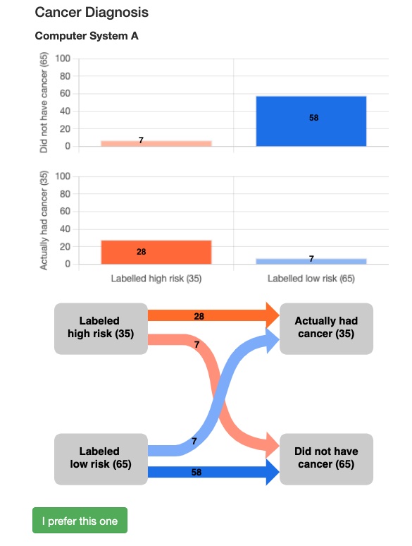
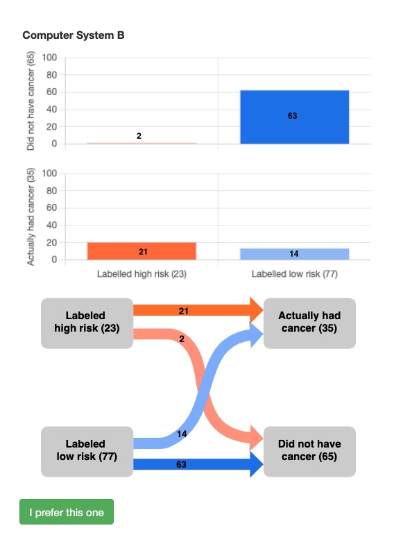
Figure 2: Proposed visualization for the pairwise comparison of confusion matrices. The web UI asks for a few comparison queries of such type to the subjects and uses their real-time responses to elicit their metrics.

Our proposed UI starts with a questionnaire asking about demographic information including expertise in machine learning and healthcare. The UI then broadly has three parts outlined as follows:

Phase-I: Understanding the Visualizations. The UI first describes the task of cancer diagnosis and how classifiers can be inaccurate in their predictions. Then, it shows a few confusion matrices and asks questions related to comprehension, comparison, and simulation (see Table 1 in [11]) in the context of cancer diagnosis. This phase familiarize the subjects with the visualizations.

Phase-II: Eliciting Linear Metrics. This phase ask subjects for pairwise preferences over confusion matrices and implement the binary-search based procedure, i.e., Algorithm 1 in [3]. In this work, we fix the stopping parameter $\epsilon$ to $0.05$. The UI takes in real-time responses of the subjects reflecting on their trade-off between True Positives and True Negatives, generates next set of queries based on the current responses, and converge to a linear performance metric at the back end.

Phase-III: Random Comparisons for Evaluation. For evaluation purposes, the third phase asks for pairwise preferences on a random set of queries right after the binary search algorithm has converged, and we have elicited the metric. The subjects are not made aware of this information and are shown queries in continuation to the previous phase.

5 User Study and Results

We recruited ten subjects for the study whose demographics are shown in Table 2. The study was approved by IRB at University of Illinois. The study was conducted over a video call, where the participants were asked to share the screen after they had filled the questionnaire. After the elicitation task, we asked think-aloud style interview questions, which are shown in Table 2.

5.1 Quantitative Results and Findings

Once the UI elicits the subject’s linear performance metric in Phase-II, it asks for fifteen random queries for evaluation in Phase-III. We measure the fraction of times our elicited metric’s preferences matches with the subject’s preferences over the fifteen queries in Phase-III, i.e.,

$${\cal M}\mathrel{\mathop{\ordinarycolon}}=\frac{\sum_{i=1}^{15}{\mathbf{1}}[\text{subject's preference }==\text{metric's preference for query }i]}{15}\times 100.$$

We show the elicited metric for the ten subjects and the ${\cal M}$ values in Table 4. We see for nine out of ten subjects that more than 85% of the times our elicited metric’s preferences matches with the subject’s preferences on the fifteen evaluation queries. The absolute ${\cal M}$ measure suggest that our approach is effective; however, without comparing to a baseline, it is not yet known how effective it really is. In future, we plan to develop a baseline for comparison on the ME task using the measure ${\cal M}$.

5.2 Qualitative Feedback and Guidelines for the Future

We now summarize feedback observed during the user study and the findings from the interviews. We also formulate guidelines for future research on practical ME, which are shown in Table 4.

Observations during study sessions: We noted that subjects were not comfortable in answering the simulation-based questions in Phase-I of the UI (Section 4). A possible reason could be that the direction of the flow-chart is opposite to the conditioning of probability that is asked in those questions (G1, Table4). While comparing confusion matrices, we also noted that after a few rounds, the subjects tend to look at only the flow-charts for comparison (G2, Table4).

Table 1: Subjects’ demographics: The values in parenthesis show the number of subjects. ML and Healthcare stand for ML and healthcare knowledge, respectively.

Age	Education	ML	HC
25(2)	Grad. Col.(4)	None(5)	None(5)
26(3)	Masters(3)	Begin.(3)	Some(2)
28(5)	Ph.D.(3)	Intermed.(2)	No resp.(3)

Table 2: Post-task interview questions.

Q1	What do you think is worse: (a) Large number of patients that actually have cancer but are labelled as low risk, or (b) Large number of patients that do not have cancer but are labelled as high risk.
Q2	Could you quantify how much worse the chosen option is in comparison to the other? Why or why not? Could you quantify this? i.e, 10x worse for me
Q3	For the questions presented in this task, how did you decide which system you would prefer your doctor to use?
Q4	What was difficult about making these choices?
Q5	What additional information would have helped you to make these choices?
Q6	Do you have any feedback for us on your experience today?

Table 3: Elicited metrics for the subjects along with ${\cal M}$.

S	Metrics	${\cal M}$
S1	0.125 TN + 0.875 TP	87
S2	0.141 TN + 0.859 TP	100
S3	0.125 TN + 0.875 TP	93
S4	0.141 TN + 0.859 TP	100
S5	0.328 TN + 0.672 TP	73
S6	0.031 TN + 0.969 TP	87
S7	0.031 TN + 0.969 TP	100
S8	0.359 TN + 0.641 TP	87
S9	0.125 TN + 0.875 TP	93
S10	0.141 TN + 0.859 TP	87

Table 4: Guidelines for ME.

G1	The direction in the flow-chart can be swapped with total number of labels shown in the left column and total predictions on the right.
G2	Showing only flow-chart for pairwise comparisons is better than showing flow-chart and bar-chart together.
G3	Corresponding to the post-task interview question 2, one needs to devise a UI so to ask for the intuitive guess for the false negative cost. This would also act as a baseline method for evaluation purposes as discussed in Section 5.1.
G4	In addition to confusion entries such as true positives, one should show percentages conditioned on the true classes, i.e., true positive rates.
G5	Extend the description of the associated subjective costs for the incorrect predictions (e.g., financial, emotional, etc.) from the task perspective.

Post-task interview sessions: In response to Q1 (Table 2), every subject clearly figured out the direction of the costs. However, none of the subjects could answer Q2 (Table 2) with full confidence. This further suggests the effectiveness of the ME framework. The subjects agreed that it is easier to compare two confusion matrices using the proposed UI than to directly quantify the costs (G3, Table4). In response to Q5 (Table 2), subjects mentioned that having quantities such as true positive rate in addition to true positives, would be helpful in making comparisons (G4, Table4). Lastly, subjects mentioned that it would have been easier to compare if some subjective description of the associated costs for incorrect predictions were provided in the beginning of the study (G5, Table4).

6 Conclusion

We created a web user-interface to practically elicit user performance metrics in a binary classification setting. Via a user study with ten subjects, we demonstrated an implementation of the metric elicitation procedure from [3] that makes use of the real-time user responses. We also proposed an evaluation scheme to judge the quality of the recovered metric. Lastly, using the study findings, we formulated guidelines for practical implementation of the ME framework.

The following procedure is borrowed from [3] and described here for completeness.

Algorithm 1 Linear Performance Metric Elicitation

1:  Input: Binary-search tolerance $\epsilon>0$, oracle $\Omega(\cdot,\cdot\,;\,\phi^{\text{lin}})$ with metric $\phi^{\text{lin}}$

2:  Set $\tau^{(a)}=0$ and $\tau^{(b)}=1$

3:  while $\mathinner{\!\left\lvert\tau^{(b)}-\tau^{(a)}\right\rvert}>\epsilon$ do

4:     Set $\tau^{(c)}=\frac{3\tau^{(a)}+\tau^{(b)}}{4}$, $\tau^{(d)}=\frac{\tau^{(a)}+\tau^{(b)}}{2}$, and $\tau^{(e)}=\frac{\tau^{(a)}+3\tau^{(b)}}{4}$.

5:     Set $\mkern 1.5mu\overline{\mkern-1.5mu\mathbf{c}}^{(a)},\mkern 1.5mu\overline{\mkern-1.5mu\mathbf{c}}^{(c)},\mkern 1.5mu\overline{\mkern-1.5mu\mathbf{c}}^{(d)},\mkern 1.5mu\overline{\mkern-1.5mu\mathbf{c}}^{(e)},$ and $\mkern 1.5mu\overline{\mkern-1.5mu\mathbf{c}}^{(b)}$ to be the confusion matrices corresponding to the thresholds $\tau^{(a)},\tau^{(c)}$, $\tau^{(d)}$, $\tau^{(e)}$, and $\tau^{(b)}$, respectively.

6:     Query $\Omega(\mkern 1.5mu\overline{\mkern-1.5mu\mathbf{c}}^{(c)},\mkern 1.5mu\overline{\mkern-1.5mu\mathbf{c}}^{(a)}),\quad\Omega(\mkern 1.5mu\overline{\mkern-1.5mu\mathbf{c}}^{(d)},\mkern 1.5mu\overline{\mkern-1.5mu\mathbf{c}}^{(c)})$,     $\Omega(\mkern 1.5mu\overline{\mkern-1.5mu\mathbf{c}}^{(e)},\mkern 1.5mu\overline{\mkern-1.5mu\mathbf{c}}^{(d)}),\quad\Omega(\mkern 1.5mu\overline{\mkern-1.5mu\mathbf{c}}^{(b)},\mkern 1.5mu\overline{\mkern-1.5mu\mathbf{c}}^{(e)})$.

7:     $[\tau^{(a)},\tau^{(b)}]\leftarrow$ ShrinkInterval (based on user responses){see Figure 3}

8:  Set $\tau^{(d)}=\frac{1}{2}(\tau^{(a)}+\tau^{(b)})$

9:  Output: $\tau^{(d)}$

The ShrinkInterval subroutine (illustrated in Figure 3) is binary-search based routine that shrinks the interval $[\tau^{(a)},\tau^{(b)}]$ by half based on the oracle responses to four queries.

Subroutine ShrinkInterval
Input: Oracle responses for $\Omega(\mkern 1.5mu\overline{\mkern-1.5mu\mathbf{c}}^{(c)},\mkern 1.5mu\overline{\mkern-1.5mu\mathbf{c}}^{(a)})$,
$\Omega(\mkern 1.5mu\overline{\mkern-1.5mu\mathbf{c}}^{(d)},\mkern 1.5mu\overline{\mkern-1.5mu\mathbf{c}}^{(c)}),$ $\Omega(\mkern 1.5mu\overline{\mkern-1.5mu\mathbf{c}}^{(e)},\mkern 1.5mu\overline{\mkern-1.5mu\mathbf{c}}^{(d)}),\Omega(\mkern 1.5mu\overline{\mkern-1.5mu\mathbf{c}}^{(b)},\mkern 1.5mu\overline{\mkern-1.5mu\mathbf{c}}^{(e)})$
If   ($\mkern 1.5mu\overline{\mkern-1.5mu\mathbf{c}}^{(a)}\succ\mkern 1.5mu\overline{\mkern-1.5mu\mathbf{c}}^{(c)}$) Set $\tau^{(b)}=\tau^{(d)}$.
elseif   ($\mkern 1.5mu\overline{\mkern-1.5mu\mathbf{c}}^{(a)}\prec\mkern 1.5mu\overline{\mkern-1.5mu\mathbf{c}}^{(c)}\succ\mkern 1.5mu\overline{\mkern-1.5mu\mathbf{c}}^{(d)}$) Set $\tau^{(b)}=\tau^{(d)}$.
elseif   ($\mkern 1.5mu\overline{\mkern-1.5mu\mathbf{c}}^{(c)}\prec\mkern 1.5mu\overline{\mkern-1.5mu\mathbf{c}}^{(d)}\succ\mkern 1.5mu\overline{\mkern-1.5mu\mathbf{c}}^{(e)}$) Set $\tau^{(a)}=\tau^{(c)}$, $\tau^{(b)}=\tau^{(e)}$.
elseif   ($\mkern 1.5mu\overline{\mkern-1.5mu\mathbf{c}}^{(d)}\prec\mkern 1.5mu\overline{\mkern-1.5mu\mathbf{c}}^{(e)}\succ\mkern 1.5mu\overline{\mkern-1.5mu\mathbf{c}}^{(b)}$) Set $\tau^{(a)}=\tau^{(d)}$.
else Set $\tau^{(a)}=\tau^{(d)}$.
Output: $[\tau^{(a)},\tau^{(b)}]$.

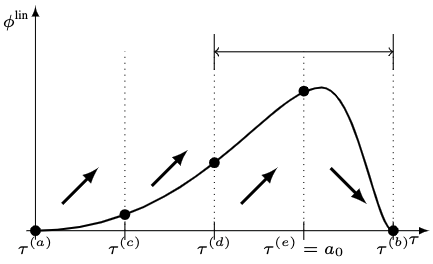
Figure 3: (Left): The ShrinkInterval subroutine used in line 7 of Algorithm 1 (Right): Visual illustration of the subroutine ShrinkInterval; ShrinkInterval shrinks the current search interval to half based on oracle responses to four queries.

References

- [1] Pavel Dmitriev and Xian Wu. Measuring metrics. In CIKM, 2016.
- [2] Ashutosh Kumar Dubey, Umesh Gupta, and Sonal Jain. Analysis of k-means clustering approach on the breast cancer wisconsin dataset. International journal of computer assisted radiology and surgery, 11(11):2033–2047, 2016.
- [3] Gaurush Hiranandani, Shant Boodaghians, Ruta Mehta, and Oluwasanmi Koyejo. Performance metric elicitation from pairwise classifier comparisons. In The 22nd International Conference on Artificial Intelligence and Statistics, pages 371–379, 2019.
- [4] Gaurush Hiranandani, Shant Boodaghians, Ruta Mehta, and Oluwasanmi O Koyejo. Multiclass performance metric elicitation. In Advances in Neural Information Processing Systems, pages 9351–9360, 2019.
- [5] Gaurush Hiranandani, Jatin Mathur, Harikrishna Narasimhan, and Oluwasanmi Koyejo. Quadratic metric elicitation for fairness and beyond. In Uncertainty in Artificial Intelligence, pages 811–821. PMLR, 2022.
- [6] Gaurush Hiranandani, Harikrishna Narasimhan, and Oluwasanmi Koyejo. Fair performance metric elicitation. In NeurIPS, 2020.
- [7] Oluwasanmi O Koyejo, Nagarajan Natarajan, Pradeep K Ravikumar, and Inderjit S Dhillon. Consistent binary classification with generalized performance metrics. In NIPS, pages 2744–2752, 2014.
- [8] Riccardo Mazza. Introduction to information visualization. Springer Science & Business Media, 2009.
- [9] Harikrishna Narasimhan, Rohit Vaish, and Shivani Agarwal. On the statistical consistency of plug-in classifiers for non-decomposable performance measures. In Advances in Neural Information Processing Systems, pages 1493–1501, 2014.
- [10] Buyue Qian, Xiang Wang, Fei Wang, Hongfei Li, Jieping Ye, and Ian Davidson. Active learning from relative queries. In IJCAI, pages 1614–1620, 2013.
- [11] Hong Shen, Haojian Jin, Ángel Alexander Cabrera, Adam Perer, Haiyi Zhu, and Jason I Hong. Designing alternative representations of confusion matrices to support non-expert public understanding of algorithm performance. Proceedings of the ACM on Human-Computer Interaction, 4(CSCW2):1–22, 2020.
- [12] Sitan Yang and Daniel Q Naiman. Multiclass cancer classification based on gene expression comparison. Statistical applications in genetics and molecular biology, 13(4):477–496, 2014.
- [13] Yunfeng Zhang, Rachel Bellamy, and Kush Varshney. Joint optimization of ai fairness and utility: A human-centered approach. In Proceedings of the AAAI/ACM Conference on AI, Ethics, and Society, pages 400–406, 2020.
Appendix for “Metric Elicitation; Moving from Theory to Practice”