Guan, Basciftci, and Van Hentenryck

Iterative Algorithms for ODMTS-DA Problem

Heuristic Algorithms for Integrating Latent Demand
into the Design of
Large-Scale On-Demand Multimodal Transit Systems

Hongzhao Guan H. Milton Stewart School of Industrial and Systems Engineering, Georgia Institute of Technology, hguan7@gatech.edu, Beste Basciftci Department of Business Analytics, Tippie College of Business, University of Iowa, beste-basciftci@uiowa.edu, Pascal Van Hentenryck H. Milton Stewart School of Industrial and Systems Engineering, Georgia Institute of Technology, pascal.vanhentenryck@isye.gatech.edu,

Capturing latent demand has a pivotal role in designing public transit services: omitting these riders can lead to poor quality of service and/or additional costs. This paper explores this topic in the design of On-Demand Multimodal Transit Systems with Rider Adoptions (ODMTS-DA). Prior work proposed a bilevel optimization model between the transit agency and riders with choice of adoption, and an exact algorithm to solve the resulting ODMTS-DA design problem. However, due to the complexity and combinatorial nature of the ODMTS-DA, the exact algorithm exhibits difficulties on large-scale instances. This paper aims at addressing this challenge in order to find high-quality ODMTS-DA designs in reasonable time. It proposes five heuristic algorithms whose designs are driven by fundamental properties of optimal solutions. The performance of the heuristic algorithms are demonstrated on two test cases leveraging real data: a medium-size case study for the Ann Arbor and Ypsilanti region in the state of Michigan and a large-scale case study conducted in the Atlanta metropolitan region in the state of Georgia. To evaluate the results, besides directly comparing computational times and optimality gaps with the exact algorithm, this paper introduces two additional metrics that leverage the characteristics of optimal solutions with respect to customer adoption. Computational results demonstrate that the heuristic algorithms find optimal solutions for medium-size problem in short running times, and discover high-quality solutions to the large-case study that improve upon the best solution found by the exact algorithm in considerably less time. The ODMTS designs obtained by these algorithms provide substantial benefits in terms of convenience, operating cost, and carbon emissions.

transit network optimization, algorithm design, heuristics, latent demand, on-demand services

1 Introduction

On-Demand Multimodal Transit Systems (ODMTS) are transit systems that tightly integrate on-demand shuttles with fixed transit services such as high-frequency buses and urban rail systems. ODMTS are operated around a number of hubs that serve as stops for buses and rail. The on-demand shuttles are primarily employed as the feeders to the hubs and represents an effective solution to the first-and-last-mile problem faced by most of the transit agencies. Several simulation studies have demonstrated that ODMTS can provide considerable cost and convenience benefits in different cities under diverse circumstances (Mahéo, Kilby, and Van Hentenryck 2019, Dalmeijer and Van Hentenryck 2020, Auad et al. 2021). Although the problem settings are varied, these studies aim at the same objective: to redesign transit systems with ODMTS, while solely considering the existing transit users and neglecting potential riders that could adopt the system.

The motivation of this paper stems from a concern of transit agencies: how to ensure that the ODMTS design will capture ridership accurately and, in particular, customer adoption. Indeed, a system designed with only existing ridership might lead to suboptimal ODMTS designs with poor quality of service in areas where adoption increases and/or costs increase as the on-demand shuttles are used too extensively. In the context of ODMTS, two previous studies addressed this concern by modeling the problem with bilevel optimization frameworks (Basciftci and Van Hentenryck 2020, 2022). These frameworks establish a game between the transit agency and the potential new users, e.g., commuters who normally commute with their personally-owned vehicles. In particular, the agency proposes an ODMTS service and optimal routes for each user under the current design; the potential riders then evaluate the convenience of these routes, and decide whether to adopt the ODMTS service. This problem setting in Basciftci and Van Hentenryck (2022) is adopted in this paper and referred to as the ODMTS Design with Adoptions (ODMTS-DA) problem.

To solve the ODMTS Design with Adoptions problem, Basciftci and Van Hentenryck (2022) proposed an exact algorithm whose resulting design can be considered as the equilibrium point of the game between the transit agency and the potential transit users. The effectiveness of this exact algorithm was demonstrated in a case study conducted in Ann Arbor and Ypsilanti area in Michigan, USA. Nevertheless, this exact algorithm becomes computationally challenging on large-scale instances coming from cities such as Atlanta. Furthermore, due to the complexity of the exact algorithm, it is even practically challenging to obtain high-quality, sub-optimal solutions on large-scale problems. This paper thus explores whether heuristics can provide fast approximations to the optimal solutions of large-scale instances.

This paper first identifies the structural properties of the optimal solution of the ODMTS-DA problem, in terms of the adoption behavior. Then, the paper presents an alternative framework to significantly reduce the problem complexity by splitting the original bilevel framework into two components: (i) a regular ODMTS design problem without rider adoption as described in Mahéo, Kilby, and Van Hentenryck (2019) and (ii) an evaluation component that uses the ODMTS choice model to capture the adoption behavior and decides the set of riders and the network to be used in the next iteration. The heuristic algorithms combine these two components by increasing incrementally the sets of riders to be considered in the design and/or by progressively adding more fixed routes in the design.

More precisely, the paper proposes five heuristic algorithms to approximate the optimal solution of the ODMTS-DA problem. The differences among these algorithms mostly occur at the transitions between these two primary steps, e.g, how they reshape the demand data and how they fix certain arcs in the network. The effectiveness of these five heuristics algorithms is evaluated on two case studies and compared with the exact algorithm. In addition to the optimality gap that can be used for evaluating the computational performance of the algorithms, this paper further proposes new metrics that assess the quality of the ODMTS design by measuring the trade-off between the transit agency and the potential new users based on the properties of optimal solutions. The primary contributions of this study can be summarized as follows:

1. The paper presents adoption properties satisfied by optimal solutions of the ODMTS-DA problem. The properties are then used for the design of the heuristic algorithms and the definition of new metrics—False Rejection Rate and False Adoption Rate. The metrics give new insights on the quality of ODMTS designs and provide guidelines for the transit agencies in selecting a desirable design.

2. This paper proposes five iterative algorithms to efficiently approximate optimal solutions of the ODMTS-DA problem and discusses their structural properties. The algorithms are designed to address the problem under varied circumstances, including different demand distributions and backbone lines (e.g., existing rail system) coverage.

3. This paper demonstrates the advantages of using the heuristic algorithms by conducting two comprehensive case studies constructed from real data—(i) the transit system of the Ann Arbor and Ypsilanti region in the state of Michigan and (ii) the much larger transit system of the Atlanta metropolitan region in the state of Georgia. The results show that the heuristic algorithms (almost always) quickly find the optimal solution for the first case study. Moreover, in the Atlanta case study, the heuristic algorithms find better solutions than the exact algorithm in a fraction of the time while satisfying certain adoption properties of the optimal solutions.

The remaining of this paper is organized as follows: Section 2 first presents the related work in ODMTS and its connection with travel mode choices and then discusses the use of heuristic algorithms on different mobility problems. Section 3 introduces the ODMTS-DA problem. The five iterative algorithms are introduced in Section 4. The two case studies are discussed in Sections 5 and 6. The conclusion and future research directions are discussed in Section 7.

2 Related Literature

The design of ODMTS stems from the multi-modal hub location and hub network design problem proposed by Alumur, Kara, and Karasan (2012). Mahéo, Kilby, and Van Hentenryck (2019) first introduced the ODMTS by utilizing the concept of on-demand shuttles and constructing a hub-to-hub network design that is fed by these shuttles. Dalmeijer and Van Hentenryck (2020) further extended the ODMTS by considering varied bus arc frequencies, passenger transfer limit, and backbone transit lines. All of the studies aim at discovering a design that minimizes a weighted combination of the transit system operating cost and passenger convenience. However, none of these studies integrates latent demand within the proposed optimization models. The ODMTS Design with Fixed Demand problem is referred to as the ODMTS-DFD problem in this paper and its presented in later sections.

As articulated by Schöbel (2012), many existing methods for transit network design problems are based on the assumption that the passenger demand is known and fixed. Thus, contrary to the abovementioned studies, other studies have considered design/planning problems together with latent demand—potential customers who might be attracted by the proposed solutions. Klier and Haase (2008) presented an optimization model without a fixed demand by employing a linear demand function of the expected travel time to model its impact on transit demand. In another study, while maximizing the number of expected passengers, the same authors employed a logit model to estimate the mode choice between the best transit route and an alternative travel mode (Klier and Haase 2015). A series of studies presented by Canca et al. comprehensively addressed this problem. Their first study introduced a model that simultaneously determines the network design, line planning, capacity, fleet investment, and passengers mode and route choices (Canca et al. 2016). Later on, two follow-up studies proposed adaptive large neighborhood search metaheuristics to solve variations of this model over large-scale data, respectively (Canca et al. 2017, 2019). Furthermore, another system incorporating line planning and travel behavior is proposed by Hartleb et al. (2021). The authors utilized a mixed-integer linear program for line planning while capturing mode and route choices from a customer’s perspective. The mode choice function is a logit model which decides if a traveler takes public transit.

Among the studies that consider latent ridership, the first systematic study of ODMTS with rider adoption awareness was reported by Basciftci and Van Hentenryck (2020). This study indicates that a bilevel optimization framework needs to be utilized to model the problem to ensure a fair design for the transit system, and the optimization model includes a personalized choice model which associates adoption choices with the time and cost of trips in the ODMTS. In a follow-up study, the choice model was then redesigned such that the rider preferences solely depend on trip convenience under a fixed pricing strategy of the transit agency (Basciftci and Van Hentenryck 2022). Together these two studies provide significant insights into the design of exact algorithms that decompose and solve the problem under different choice model assumptions. Moreover, detailed case studies with realistic data are also conducted to demonstrate the advantages and practicability of the bilevel approaches and the exact algorithms. However, the combinatorial nature of the exact algorithms present a significant challenge for solving large-scale ODMTS-DA problems. In order to overcome this challenge, this paper proposes several heuristics that iteratively solve the problem while considering the ODMTS-DFD problem and the choice model separately.

In general, iterative approaches are widely applied to the field of transportation science, especially for complex large-scale problems. For example, the following studies investigated iterative approaches on problems related to large-scale network design such as designing distribution networks and planning public transit for large urban areas (Gattermann, Schiewe, and Schöbel 2016, Schöbel 2017, Cipriani, Gori, and Petrelli 2012, Liu et al. 2021). Overall, these studies highlight the efficiency of using iterative algorithms when designing large-scale logistic networks and urban transit networks. When expanding the network design problem from city-wise to country-wise, another example of using iterative approaches to solve large-scale public transit problems is the study presented by Liu et al. (2019). Similar to ODMTS, the goal of the problem is to optimize both the operational costs and passenger travel convenience. However, instead of using time to directly measure travel convenience, a conversion from travel time to operational income is utilized. Two case studies using the Chinese high-speed rail data presented by the authors demonstrate that iterative algorithms can efficiently solve large-scale public transit planning problems while providing a more profitable solution. Furthermore, iterative approaches are utilized to solve more general network design problems such as the incomplete hub location problems—selecting hub locations without the restriction of fully-connected networks (Dai et al. 2019) and the fleet assignment problem—assigning a fleet while maximizing expected revenue (Dumas, Aithnard, and Soumis 2009). The latter study inspired Kroon, Maróti, and Nielsen (2015), and they proposed a three-step iterative approach to optimize the rolling stock to the disrupted passenger flows.

Besides designing public transit networks, iterative approaches are also applied to other topics in the field of transportation science when the original problem has a bilevel nature. Yu, Yang, and Yao (2010) first proposed a bilevel optimization model to determine the optimal bus frequencies to minimize the total passengers’ travel time, and an iterative algorithm that consists of a genetic algorithm and a label-marking method is then proposed to solve this model. Tawfik, Gendron, and Limbourg (2021) provided another example of applying iterative algorithms on bilevel problems by continuing on a previous study where a bilevel model formulates service design and pricing for freight networks (Tawfik and Limbourg 2019). Lodi et al. (2016) studied game theoretic frameworks between the transit agency and bus operators for optimizing certain contractual relationships in public transit systems, and employed iterative schemes as part of their solution procedure.

So far, not much attention has been paid to the role of iterative algorithms when integrating public transit planning and passenger mode choices. One of the earliest approaches is presented by Lee and Vuchic (2005). They consider a transit network design problem with variable transit demand under a given fixed total demand that can be split into transit mode or auto mode, and this setting is also adopted by Fan and Machemehl (2006) within a genetic algorithm. The approaches used by these studies share two similarities with the study described in this paper—(i) the transit demand is variable such that riders can choose between transit services and personally-owned vehicles and (ii) at each iteration, the algorithm reshapes the transit demand then redesigns the transit network. On the other hand, this paper proposes a systematic approach for integrating rider preferences into the ODMTS-DFD problem by introducing five iterative algorithms and leveraging the bilevel nature of the original problem. Three of these algorithms are driven by modifying trip sets considered in each iteration, whereas the other two are mainly driven by arc selection in the network. Furthermore, beside efficiently solving this large-scale problem, the iterative algorithms in this study also bring novelties by providing ODMTS designs with guaranteed adoption and rejection properties that are practically useful to transit agencies.

3 ODMTS Design with Adoptions

This section introduces the primary problem of this study—the ODMTS Design with Adoptions (ODTMS-DA) problem. The motivation for this problem stems from the desire to establish an ODMTS that concurrently serves the existing transit users and captures latent demand. This section presents a bilevel optimization framework for capturing the travel mode adoption in the ODMTS design by considering the existing transit riders and potential riders that can adopt the transit system. The leader problem corresponds to the transit agency, which aims at designing the ODMTS, i.e., determining which hub legs are connected to each other under cost, convenience and adoption considerations. Given the transit network design, each follower problem identifies the most cost-efficient and convenient route from an origin to a destination, and proposes these routes to the corresponding riders. Subsequently, the potential riders determine their mode decisions by taking into account the properties of the resulting routes and their own preferences.

The optimization model considers a set of nodes $N$, that represents the stops. A subset of these nodes $H\subseteq N$ corresponds to the hubs that can be stops for high-frequency buses or rail services (without loss of generality, the paper only uses buses in the formalization for conciseness). Each trip $r\in T$ is characterized by an origin stop $or^{r}\in N$, a destination stop $de^{r}\in N$, and a number of riders $p^{r}\in\mathbb{Z}_{+}$. Given stops $i,j\in N$, the time and distance between these stops are given by $t_{ij}$ and $d_{ij}$, respectively. To have a weighted objective considering both convenience and cost aspects of the ODMTS design, a parameter $\theta\in[0,1]$ is defined such that the trip duration associated with convenience are multiplied by $\theta$ and costs are multiplied by $1-\theta$. In particular, the transit agency incurs a weighted investment and operational cost $\beta_{hl}=(1-\theta)b_{dist}\,n\,d_{hl}$ if the leg between hubs $h,l\in H$ is open, where $b_{dist}$ is the cost of using a bus per kilometer and $n$ is the number of buses operating in each open leg within the planning horizon. The investment cost $\beta_{hl}$ can also be modeled by $\beta_{hl}=(1-\theta)b_{time}\,n\,t_{hl}$ where $b_{time}$ stands for the cost of operating a bus per hour. The transit agency has the freedom to determine the more suitable modeling method. For each trip $r\in T$, the transit agency incurs a weighted inconvenience cost $\tau^{r}_{hl}=\theta(t_{hl}+t_{hl}^{wait})$ for the parts of the trips traveled by buses, where $t_{hl}^{wait}$ is the average waiting time of a passenger for the bus between hubs $h$ and $l$. For the legs of the trips traveled by on-demand shuttles, the transit agency incurs a weighted cost and inconvenience cost $\gamma_{ij}^{r}=(1-\theta)\omega\,d_{ij}+\theta t_{ij}$ for each trip $r\in T$, where $\omega$ is the cost of using a shuttle per kilometer. The transit agency charges riders a fixed cost $\phi$ to use the ODMTS, irrespective of their routes. Thus, the fixed value $\varphi=(1-\theta)\phi$ becomes an additional revenue to the transit agency for riders adopting the ODMTS.

The bilevel optimization model uses binary variable $z_{hl}$ whose value is 1 if the leg between the hubs $h,l\in H$ is open. For each trip $r\in T$, the model uses binary variables $x_{hl}^{r}$ and $y_{ij}^{r}$ to determine whether this trip utilizes the leg between the hubs $h,l\in H$, and the shuttle leg between the stops $i,j\in N$, respectively. To integrate the choices of the riders into the planning, the trips in $T^{\prime}\subseteq T$ are associated with riders who have their personal vehicles; these riders can decide whether to adopt the ODMTS, based on the route defined by variables $\mathbf{x^{r}}$ and $\mathbf{y^{r}}$. The choice function ${\cal C}^{r}(\mathbf{x^{r}},\mathbf{y^{r}})$ of trip $r\in T^{\prime}$ depends on the route features, such as the trip duration. These features are used in the function $f^{r}(\mathbf{x^{r}},\mathbf{y^{r}})$ that returns a scalar value that can be compared with a threshold value in the choice function ${\cal C}^{r}(\mathbf{x^{r}},\mathbf{y^{r}})$. In particular, given the fixed pricing strategy, the adoption behavior of the riders can be expressed in terms of the duration of the trips through the function

$$f^{r}(\mathbf{x^{r}},\mathbf{y^{r}})=\sum_{h,l\in H}(t_{hl}+t_{hl}^{wait})x_{hl}^{r}+\sum_{i,j\in N}t_{ij}y_{ij}^{r}.$$ (1)

By comparing the trip duration in ODMTS with the direct trip duration $t^{r}_{cur}$ with personal vehicles through a parameter $\alpha^{r}\geq 1$, the choice function can be expressed as follows:

$${\cal C}^{r}(\mathbf{x^{r}},\mathbf{y^{r}})\equiv\mathbbm{1}(f^{r}(\mathbf{x^{r}},\mathbf{y^{r}})\leq\alpha^{r}\ t^{r}_{cur}).$$ (2)

To utilize the output of this choice model, the model uses a binary decision variable $\delta^{r}$ for each trip $r\in T^{\prime}$ whose value is 1 if the riders of that trip prefers adopting ODMTS. The remaining trips $T\setminus T^{\prime}$ correspond to the set of existing riders, who are assumed to continue choosing the ODMTS. This is justified by the case study in Basciftci and Van Hentenryck (2022) that demonstrated the improvement in convenience of the suggested routes compared to the existing transit system.

Figure 1 presents the bilevel optimization model. The leader problem (Equations (3a)–(3e)) designs the network between the hubs for the ODMTS, whereas the follower problem (Equations (4a)–(4f)) obtains routes for each trip $r\in T$ by considering the legs of the network design and the on-demand shuttles to serve the first and last miles of the trips.

$$\min_{z_{hl},\delta^{r}}\quad \sum_{h,l\in H}\beta_{hl}z_{hl}+\sum_{r\in T\setminus T^{\prime}}p^{r}g^{r}+\sum_{r\in T^{\prime}}p^{r}\delta^{r}(g^{r}-\varphi)$$ (3a)

s.t. $$\sum_{l\in H}z_{hl}=\sum_{l\in H}z_{lh}\quad\forall h\in H$$ (3b)

$$\delta^{r}={\cal C}^{r}(\mathbf{x^{r}},\mathbf{y^{r}})\quad\forall r\in T^{\prime}$$ (3c)

$$z_{hl}\in\{0,1\}\quad\forall h,l\in H$$ (3d)

$$\delta^{r}\in\{0,1\}\quad\forall r\in T^{\prime}$$ (3e)

where $(\mathbf{x^{r}},\mathbf{y^{r}},g^{r})$ are a solution to the optimization problem

$$\operatorname*{lex-min}_{x_{hl}^{r},y_{ij}^{r},g^{r},f^{r}}\quad \langle g^{r},f^{r}\rangle$$ (4a)

s.t. $$g^{r}=\sum_{h,l\in H}\tau_{hl}^{r}x_{hl}^{r}+\sum_{i,j\in N}\gamma_{ij}^{r}y_{ij}^{r}$$ (4b)

$$f^{r}=\sum_{h,l\in H}(t_{hl}+t_{hl}^{wait})x_{hl}^{r}+\sum_{i,j\in N}t_{ij}y_{ij}^{r}$$ (4c)

$$\sum_{\begin{subarray}{c}h\in H\\ \text{if }i\in H\end{subarray}}(x_{ih}^{r}-x_{hi}^{r})+\sum_{i,j\in N}(y_{ij}^{r}-y_{ji}^{r})=\begin{cases}1&,\text{if }i=or^{r}\\ -1&,\text{if }i=de^{r}\\ 0&,\text{otherwise}\end{cases}\quad\forall i\in N$$ (4d)

$$x_{hl}^{r}\leq z_{hl}\quad\forall h,l\in H$$ (4e)

$$x_{hl}^{r}\in\{0,1\}\quad\forall h,l\in H,y_{ij}^{r}\in\{0,1\}\quad\forall i,j\in N.$$ (4f)

Figure 1: The Bilevel Optimization Model for ODMTS Design with Adoption (ODMTS-DA).

The objective of the leader problem (3a) minimizes the sum of (i) the investment cost of opening bus legs and (ii) the weighted cost and inconvenience of the trips of the existing riders, minus (iii) the revenues of the riders with choice that are adopting the ODMTS. Constraint (3b) ensures weak connectivity between the hubs with the same number of incoming and outgoing open legs. A network design is represented by vector $\mathbf{z}\in\{0,1\}^{|H|\times|H|}$ which satisfies this weak connectivity constraint. Constraint (3c) represents the mode choice of the riders in $T^{\prime}$ depending on the ODMTS routes.

For each trip $r$, the objective of the follower problem (4) minimizes the lexicographic objective function $\langle g^{r},f^{r}\rangle$, where $g^{r}$ corresponds to the cost and inconvenience of trip $r$ and $f^{r}$ breaks potential ties between the solutions with the same value of $g^{r}$ by returning the most convenient route for the rider of trip $r$, in line with feature function $f^{r}$ considered in the travel choice model (2). Since sub-objective $g^{r}$ contains both cost and inconvenience of trip $r$, $g^{r}$ includes sub-objective $f^{r}$ multiplied by $\theta$. As presented in Basciftci and Van Hentenryck (2022), for any network design, a lexicographic minimizer of the follower problem (4) exists, and the lexicographic minimum is unique. Thus, once a network design $\mathbf{z}$ is given, the values for the other decision variables, i.e., $x_{hl}^{r}$, $y_{ij}^{r}$, and $\delta^{r}$, can all be deducted. Constraint (4d) guarantees flow conservation for the bus and shuttle legs used in trip $r$ for origin, destination and each of the intermediate points utilized. Constraint (4e) ensures that the route only takes into account the open legs between the hubs. Since the follower problem has a totally unimodular constraint matrix, it can be solved as a linear program with an objective of the form $M\ g^{r}+f^{r}$ for a suitably large value of $M$. Furthermore, to limit the maximum number of transfers in each suggested route, a constraint can be added to the follower problem. As the addition of this constraint violates the totally unimodularity property, the underlying network can be remodelled through a transfer expanded graph that captures the transfer limit by design (Dalmeijer and Van Hentenryck 2020).

It is useful to revisit the intuition behind the goals of the model now that it has been presented. The transit agency first obtains the ODMTS design by considering cost and convenience aspect of the trips considered. Secondly, the follower problems determine the routes to be presented to the riders during operations. The choice function in the leader problem determines, for each rider with a mode choice, whether they would adopt the proposed route or elect to use their own vehicle. If such a rider decides to use transit, the agency receives a fixed revenue for that trip.

To solve this bilevel optimization problem, an exact decomposition algorithm was proposed in Basciftci and Van Hentenryck (2022): it combines Benders decomposition algorithm with a combinatorial cut generation procedure to integrate rider adoption constraints. Despite of addition of valid inequalities and pre-processing techniques, the algorithm encounters computational challenges for large-scale instances: it exhibits large optimality gaps and runtimes, due to the bilevel nature of this problem and the complexity arising from adoption considerations. This motivates the design of effective heuristic algorithms that can generate high-quality solutions within reasonable time limits while leveraging adoption properties of optimal solutions.

4 Iterative Algorithms

This section presents heuristic algorithms to find high-quality solutions of the OMDTS-DA problem in reasonable time. The heuristic algorithm uses, as a backbone, the ODMTS Design problem with Fixed Demand (ODMTS-DFD) which is presented in Figure 2. Compared to the ODMTS-DA, the ODMTS-DFD removes the choice function constraint (3c) and the decision variables of the form $\delta^{r}$ that correspond to the rider choices. As the latent demand is omitted in this problem setting, the additional revenue is discarded in the objective function of the leader problem. Moreover, the terms core trips and latent trips are introduced to represent existing transit trips $T\setminus T^{\prime}$ and trips with choices $T^{\prime}$ in Section 3 respectively; they are used here in order to emphasize their roles in the iterative algorithms. In particular, the heuristic algorithm will use ODMTS-DFD with a set of trips $\hat{T}\subseteq T$ that is always constructed from all core trips and a subset of the latent trips.

$$\min_{z_{hl}}\quad \sum_{h,l\in H}\beta_{hl}z_{hl}+\sum_{r\in\hat{T}}p^{r}g^{r}$$ (5a)

s.t. $$\sum_{l\in H}z_{hl}=\sum_{l\in H}z_{lh}\quad\forall h\in H$$ (5b)

$$z_{hl}\in\{0,1\}\quad\forall h,l\in H$$ (5c)

where $g^{r}$ is a solution to the optimization problem

$$\operatorname*{lex-min}_{x_{hl}^{r},y_{ij}^{r},g^{r},f^{r}}\quad \langle g^{r},f^{r}\rangle$$ (6a)

s.t. $$g^{r}=\sum_{h,l\in H}\tau_{hl}^{r}x_{hl}^{r}+\sum_{i,j\in N}\gamma_{ij}^{r}y_{ij}^{r}$$ (6b)

$$f^{r}=\sum_{h,l\in H}(t_{hl}+t_{hl}^{wait})x_{hl}^{r}+\sum_{i,j\in N}t_{ij}y_{ij}^{r}$$ (6c)

$$\sum_{\begin{subarray}{c}h\in H\\ \text{if }i\in H\end{subarray}}(x_{ih}^{r}-x_{hi}^{r})+\sum_{i,j\in N}(y_{ij}^{r}-y_{ji}^{r})=\begin{cases}1&,\text{if }i=or^{r}\\ -1&,\text{if }i=de^{r}\\ 0&,\text{otherwise}\end{cases}\quad\forall i\in N$$ (6d)

$$x_{hl}^{r}\leq z_{hl}\quad\forall h,l\in H$$ (6e)

$$x_{hl}^{r}\in\{0,1\}\quad\forall h,l\in H,y_{ij}^{r}\in\{0,1\}\quad\forall i,j\in N.$$ (6f)

Figure 2: The Optimization Model for ODMTS Design with Fixed Demand: ODMTS-DFD($\hat{T}$).

Multiple iterative algorithms are proposed in this section which can be divided into two categories: (1) trip-based iterative algorithms that present rules for constructing the trip set $\hat{T}$ at each iteration and (2) arc-based iterative algorithms that focus on obtaining network designs incrementally by fixing a set of arcs at each iteration. Since the iterative algorithms only provide an approximation to the optimal solution of ODMTS-DA and since the optimal solution might be impossible to obtain in reasonable time on large-scale instances, two key properties are introduced in this section in order to assess an ODMTS design. Ideally, one would like to obtain the design that satisfies these two properties. To this end, if the network design $\mathbf{z}$ is the optimal solution of the $\mbox{ODMTS-DFD}(\hat{T})$ problem, then it is denoted in the form $\mathbf{z}=\mbox{ODMTS-DFD}(\hat{T})$.

Property 1 (Correct Rejection)

Let $\mathbf{z}=\mbox{ODMTS-DFD}(\hat{T})$. Every rider $r\in T\setminus\hat{T}$ rejects the ODMTS option in $\mathbf{z}$.

Property 2 (Correct Adoption)

Let $\mathbf{z}=\mbox{ODMTS-DFD}(\hat{T})$. Every rider $r\in\hat{T}$ adopts the ODMTS option in $\mathbf{z}$.

When a design satisfies these two properties, it represents an equilibrium between the transit agency and the riders. The following proposition links the optimal solution $\mathbf{z}^{*}$ of ODMTS-DA and Properties 1 and 2.

Proposition 1

Assume $\mathbf{z}^{*}$ is the optimal solution of the ODMTS-DA problem (Figure 1). There exists an input trip set $\hat{T}^{*}\subseteq T$ such that $\mathbf{z}^{*}=\mbox{ODMTS-DFD}(\hat{T}^{*})$ and $\mathbf{z}^{*}$ satisfies both correct rejection and correct adoption properties (Properties 1 and 2).

Proof.

Proof: Given $\mathbf{z}^{*}$ and $\boldsymbol{\delta}^{*}$ as the optimum solution of the ODMTS-DA problem, $\hat{T}^{*}$ can be defined as $(T\setminus T^{\prime})\cup\{r\in T^{\prime}:(\delta^{r})^{*}=1\}$. ∎

The goal of the heuristic algorithm is to find the set $\hat{T}^{*}$, which is obviously challenging computationally. The algorithms proposed in this paper aim at achieving one of two different goals: (1) efficiently finding an approximation of $\hat{T}^{*}$ that satisfies the correct rejection property or correct adoption property, or (2) rapidly finding an approximation to $\mathbf{z}^{*}$ regardless of these properties. The rest of this section is organized as follows. Section 4.1 presents common concepts and notations for the heuristic algorithms. Section 4.2 and 4.3 describe the trip-based iterative algorithms and arc-based iterative algorithms, respectively. The discussion of the two properties is also presented throughout Section 4.2 and 4.3 as the iterative algorithms are introduced.

4.1 Common Concepts and Notations

This section summarizes multiple common features and notations shared by all proposed iterative algorithms. The integer $k$ is used to denote iterations. The notation $\overline{T}^{k}$ denotes the set of trips considered by the algorithm at iteration $k$, i.e., $\hat{T}=\overline{T}^{k}$ at iteration $k$. All algorithms start their first iteration by solving the problem with the core trip set $T\setminus T^{\prime}$ (the existing riders) to obtain an initial transit network design, unless specified otherwise. The latent trips are then gradually added to $\overline{T}^{k}$ over time, while the trips in the core trip set always remain in $\overline{T}^{k}$ as $k$ increases. Moreover, $\upsilon^{r}$ represents the net cost of serving a rider of trip $r$ under a given ODMTS design which is a critical factor in determining which latent trips should be considered. To this end, ${cost}(\mathbf{x^{r}},\mathbf{y^{r}})$ corresponds to the cost of the trip $r$ under the route defined by the vectors $\mathbf{x^{r}}$ and $\mathbf{y^{r}}$ in the corresponding iteration, and the net cost function of a trip can be defined as ${cost}(\mathbf{x^{r}},\mathbf{y^{r}})-\phi$ considering the fixed price $\phi$ of utilizing the transit system.

The objective function (3a) of ODMTS-DA is utilized to evaluate any ODMTS design $\mathbf{z}$ produced by ODMTS-DFD using the function

$${eval}(\mathbf{z})=\sum_{h,l\in H}\beta_{hl}z_{hl}+\sum_{r\in T\setminus T^{\prime}}p^{r}g^{r}+\sum_{r\in T^{\prime}}p^{r}\delta^{r}(g^{r}-\varphi)$$ (7a)

The input trip set to evaluate $\mathbf{z}$ is always the full trip set $T$. Therefore, the adoption decisions $\delta^{r}$ for every $r\in T^{\prime}$ are evaluated with the choice function under the ODMTS design $\mathbf{z}$ regardless of their existence in the set $\hat{T}$ used in obtaining $\mathbf{z}$.

To evaluate the quality of the ODMTS designs found by the iterative algorithms, two additional metrics, i.e., False Rejection Rate ($\%R_{false}$) and False Adoption Rate ($\%A_{false}$), are introduced to measure the violation of the correct rejection and correct adoption properties (Properties 1 and 2). These two metrics are defined as follows:

$$\%R_{false}=\cfrac{|\{r\in(T\setminus\hat{T})\cap T^{\prime}:r\text{ adopts design }\mathbf{z}\}|}{|T^{\prime}|}\times\%100$$

$$\%A_{false}=\cfrac{|\{r\in\hat{T}\cap T^{\prime}:r\text{ rejects design }\mathbf{z}\}|}{|T^{\prime}|}\times\%100$$

Here, the set $(T\setminus\hat{T})\cap T^{\prime}$ represents the set of latent trips that are not considered during the design, and the set $\hat{T}\cap T^{\prime}$ represents the latent trips considered. Core trips are excluded because they are always included in $\hat{T}$.

Remark 1

It is possible that the solution of the ODMTS-DFD with a trip set $\hat{T}\neq\hat{T}^{*}$ is a design $\mathbf{z}\neq\mathbf{z^{*}}$ that satisfies both correct rejection property and correct adoption property. Thus, satisfying both properties under an input trip set $\hat{T}$ does not necessarily imply that $\mathbf{z}$ is the optimal solution of ODMTS-DA.

Remark 2

It is possible that the optimal solution of the ODMTS-DFD with a trip set $\hat{T}\neq\hat{T}^{*}$ is the optimal design $\mathbf{z}^{*}$ of the ODMTS-DA. In other words, $\mathbf{z}^{*}$ may be discovered by a trip set $\hat{T}\neq\hat{T}^{*}$ with $\%R_{false}\neq 0$ or $\%A_{false}\neq 0$ under $\hat{T}$.

4.2 Trip-based Iterative Algorithms

This section introduces the first category of iterative algorithms—the trip-based algorithms. In general, each iteration of this type of algorithm can be summarized by three fundamental steps which are illustrated in Figure 3. The first step solves the ODMTS-DFD problem with $\hat{T}=\overline{T}^{k}$. The second step evaluates the design with Equation (7a). The third step computes the new $\overline{T}^{k+1}$ for the next iteration. All trip-based iterative algorithms have identical first and second steps. Only the third steps are different.

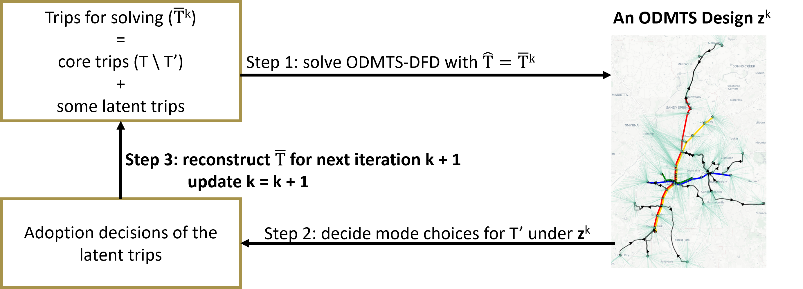
Figure 3: A flowchart that describes an iteration of the trip-based algorithms. The differences among those algorithms appear at step 3.

Three trip-based iterative algorithms are proposed. The first two are presented in Section 4.2.1 and 4.2.2. Another one combining the previous two algorithms is explained in Section 4.2.3, which enables to explore more intermediate ODMTS designs, despite of its much longer expected running time. Section 4.2.4 presents some properties of the trip-based algorithms.

4.2.1 Greedy Adoption Algorithm (LABEL:rho_GRAD)

The first trip-based iterative algorithm starts with the core trips and greedily adds adopting trips at each iteration. Algorithm LABEL:rho_GRAD maintains a set $C$ of trips and transfers latent trips from $T^{\prime}$ to $C$ at each iteration. Specifically, at a given iteration $k$, the solution $\mathbf{z}^{k}$ identifies a set of adopting trips ${T^{\prime}}_{adp}^{k}\in T^{\prime}$. It transfers $\rho$ trips from ${T^{\prime}}_{adp}^{k}$ to $C$, choosing those of least cost. This set of $\rho$ trips is denoted by ${T^{\prime}}^{k}_{\rho}$. The algorithm terminates when there are no latent trips to be absorbed by set $C$ at the end of an iteration, i.e., $|{T^{\prime}}^{k}_{\rho}|=0$. Algorithm LABEL:rho_GRAD satisfies the following property.

Proposition 2

The last ODMTS design $\mathbf{z}^{k}$ found by Algorithm LABEL:rho_GRAD with trip set $\hat{T}=\overline{T}^{k}$ satisfies the correct rejection property (Property 1).

Proof.

Proof: The last design $\mathbf{z}^{k}$ is found by solving ODMTS-DFD with $\hat{T}=(T\setminus T^{\prime})\cup C$. On completion, $|{T^{\prime}}^{k}_{\rho}|=0$ and no latent trip in $T^{\prime}\setminus C$ adopts design $\mathbf{z}^{k}$. The result follows. ∎

Algorithm 1 $\rho$-GRADrho˙GRAD

1:  Set $k=0$, $\overline{T}^{0}=T\setminus T^{\prime}$, $C=\emptyset$, unless other input values are specified.

2:  Require: step-size parameter $\rho$

3:  while True do

4:     Set $\mathbf{z}^{k}=\mbox{ODMTS-DFD}(\overline{T}^{k})$.

5:     Set $T_{check}=T^{\prime}\setminus C$.

6:     for all $r\in T_{check}$ do

7:        Set $(\mathbf{x^{r}},\mathbf{y^{r}})$ = route of $r$ under $\mathbf{z}^{k}$.

8:        Set $\delta^{r}={\cal C}^{r}(f^{r}(\mathbf{x^{r}},\mathbf{y^{r}}))$.

9:        if $\delta^{r}=1$ then

10:           Set $\upsilon^{r}$ = ${cost}(\mathbf{x^{r}},\mathbf{y^{r}})-\phi$.

11:        end if

12:     end for

13:     Set ${T^{\prime}}_{adp}^{k}=\{r\in T_{check}\mid\delta^{r}=1\}$.

14:     Set ${T^{\prime}}^{k}_{\rho}=$ the set of $\rho$ trips from ${T^{\prime}}_{adp}^{k}$with the lowest $\upsilon^{r}$.

15:     if ${T^{\prime}}_{adp}^{k}=\emptyset$ then

16:        break.

17:     else

18:        Set $C=C\cup{T^{\prime}}^{k}_{\rho}$.

19:        Set $\overline{T}^{k+1}=(T\setminus T^{\prime})\cup C$.

20:        Set $k=k+1$.

21:     end if

22:  end while

23:  return  $\mathbf{z}^{k}$

4.2.2 Greedy Rejection Algorithm (LABEL:alg:m_GRRE)

Algorithm LABEL:alg:m_GRRE greedily excludes trips from $T^{\prime}$ and introduces a growing set $R$ of rejecting trips. In addition, a variable $m$ is used to indicate how many adopting trips from $T^{\prime}\setminus R$ are included in the set $\overline{T}^{k}$ and $m$ is increased by $\eta$ at each iteration. Using $T^{\prime}\setminus R$ directly would lead to many rejections, so the algorithm proceeds carefully when choosing $\overline{T}^{k}$ early on. Algorithm LABEL:alg:m_GRRE terminates when it meets the following two conditions at an iteration $k\geq 2$:

1. the design is stable, i.e., $\mathbf{z}^{k}=\mathbf{z}^{k-1}$;

2. $m-\eta\geq|{T^{\prime}}_{adp}^{k}|$.

Note that condition 1 alone is not adequate. Indeed, in early stages, the algorithm tends to find the same design because $m$ is still relatively small. The designs found by Algorithm LABEL:alg:m_GRRE may not satisfy either of correct rejection property or correct adoption property. Instead, this algorithm is particularly designed to provide a rapid approximation.

Remark 3

Because of possible oscillations in ODMTS designs between iterations, the LABEL:alg:m_GRRE algorithm reports the design with the minimal objective instead of the last design. These oscillations occur as the set $\overline{T}^{k}$ does not monotonically increase. Note that if the last design $\textbf{z}^{k}$ is reported, then the algorithm satisfies the correct adoption property (Property 2) given that $\textbf{z}^{k}=\textbf{z}^{k-1}$.

Algorithm 2 $\eta$-GRREalg:m˙GRRE

1:  Set $k=0$, $m=0$, $R=\emptyset$, $\overline{T}^{0}=T\setminus T^{\prime}$, and $o^{*}=\infty$, unless other input values are specified.

2:  Require: step-size parameter $\eta$

3:  while True do

4:     $\mathbf{z}^{k}=\mbox{ODMTS-DFD}(\overline{T}^{k})$.

5:     if $eval(\mathbf{z}^{k})<o^{*}$ then

6:        Set $o^{*}=eval(z^{k})$.

7:        Set $\mathbf{z}_{min}=\mathbf{z}^{k}$.

8:     end if

9:     Set $T_{check}=T^{\prime}\setminus R$.

10:     for all $r\in T_{check}$ do

11:        Set $(\mathbf{x^{r}},\mathbf{y^{r}})$ = route of $r$ under $\mathbf{z}^{k}$.

12:        Set $\delta^{r}={\cal C}^{r}(f^{r}(\mathbf{x^{r}},\mathbf{y^{r}}))$.

13:        if $\delta^{r}=1$ then

14:           Set $\upsilon^{r}$ = ${cost}(\mathbf{x^{r}},\mathbf{y^{r}})-\phi$.

15:        else

16:           Set $R=R\cup\{r\}$.

17:        end if

18:     end for

19:     Set ${T^{\prime}}_{adp}^{k}=\{r\in T_{check}\mid\delta^{r}=1\}$.

20:     Set $m=m+\eta$.

21:     Set ${T^{\prime}}^{k}_{m}=$ the set of $m$ trips from ${T^{\prime}}_{adp}^{k}$with the lowest $\upsilon^{r}$.

22:     if the termination criteria is met then

23:        break.

24:     else

25:        Set $\overline{T}^{k+1}=(T\setminus T^{\prime})\cup{T^{\prime}}_{m}^{k}$;

26:        Set $k=k+1$.

27:     end if

28:  end while

29:  return  $\mathbf{z}_{min}$

4.2.3 Greedy Adoption Algorithm with Greedy Rejection Subproblem (LABEL:rho_GAGR)

Algorithm LABEL:rho_GAGR is the same as Algorithm LABEL:rho_GRAD, except that it uses Algorithm LABEL:alg:m_GRRE instead of solving ODMTS-DFD to obtain a network design. This design decision makes it possible for Algorithm LABEL:rho_GAGR to explore many more designs than Algorithm LABEL:rho_GRAD. Algorithm LABEL:rho_GAGR shares the same terminating criteria with Algorithm LABEL:rho_GRAD.

Algorithm 3 $\rho$-GAGRrho˙GAGR

1:  Set $k=0$, $C=\emptyset$, $\overline{T}^{0}=(T\setminus T^{\prime})\cup C$, and $o^{*}=\infty$.

2:  Require: step-size parameters $\rho$ and $\eta$

3:  while True do

4:     Set $\mathbf{z}^{k}={\color[rgb]{0,0,1}\textit{\nameref{alg:m_GRRE}}}$ (Algorithm LABEL:alg:m_GRRE starts from $\overline{T}^{k}$ instead of $T\setminus T^{\prime}$)

5:     if $eval(\mathbf{z}^{k})<o^{*}$ then

6:        Set $o^{*}=eval(\mathbf{z}^{k})$.

7:        Set $\mathbf{z}_{min}=\mathbf{z}^{k}$.

8:     end if

9:     Carry out steps 5—21 of LABEL:rho_GRAD

10:  end while

11:  return  $\mathbf{z}_{min}$

4.2.4 Additional Properties

This section analyzes the change in the cost and convenience of the trips, as different sets of trips are considered during ODMTS design. To this end, $g^{r}(\mathbf{z})$ is defined as the optimum cost and convenience of the trip $r$ under the network design $\mathbf{z}$.

Proposition 3

Let $\mathbf{z}^{1}=\mbox{ODMTS-DFD}(T^{1})$ and $\mathbf{z}^{2}=\mbox{ODMTS-DFD}(T^{2})$ with $T^{1}\subseteq T^{2}$. Then $\sum\limits_{r\in T^{2}\setminus T^{1}}p^{r}(g^{r}(\mathbf{z}^{2})-g^{r}(\mathbf{z}^{1}))\leq 0$.

Proof.

Proof: Note that the optimum objective function value of the network design $\mathbf{z}^{2}$ under the set of trips $T^{2}$ can be written as $\sum\limits_{h,l\in H}\beta_{hl}\mathbf{z}^{2}_{hl}+\sum\limits_{r\in T^{2}}p^{r}g^{r}(\mathbf{z}^{2})$. Since $\mathbf{z}^{1}$ is a feasible network design for this problem, the following relationship holds:

$$\sum_{h,l\in H}\beta_{hl}\mathbf{z}^{2}_{hl}+\sum_{r\in T^{2}}p^{r}g^{r}(\mathbf{z}^{2})\leq\sum_{h,l\in H}\beta_{hl}\mathbf{z}^{1}_{hl}+ \sum_{r\in T^{2}}p^{r}g^{r}(\mathbf{z}^{1})$$

$$\sum_{h,l\in H}\beta_{hl}\mathbf{z}^{2}_{hl}+\sum_{r\in T^{1}}p^{r}g^{r}(\mathbf{z}^{2})+\sum_{r\in T^{2}\setminus T^{1}}p^{r}g^{r}(\mathbf{z}^{2})\leq\sum_{h,l\in H}\beta_{hl}\mathbf{z}^{1}_{hl}+ \sum_{r\in T^{1}}p^{r}g^{r}(\mathbf{z}^{1})+\sum_{r\in T^{2}\setminus T^{1}}p^{r}g^{r}(\mathbf{z}^{1})$$

$$\sum_{h,l\in H}\beta_{hl}(\mathbf{z}^{2}_{hl}-\mathbf{z}^{1}_{hl})+\sum_{r\in T^{1}}p^{r}(g^{r}(\mathbf{z}^{2})-g^{r}(\mathbf{z}^{1}))+ \sum_{r\in T^{2}\setminus T^{1}}p^{r}(g^{r}(\mathbf{z}^{2})-g^{r}(\mathbf{z}^{1}))\leq 0$$

Following an analogous relationship by comparing the network designs under the set of trips $T^{1}$ results in

$$\sum_{h,l\in H}\beta_{hl}\mathbf{z}^{2}_{hl}+\sum_{r\in T^{1}}p^{r}g^{r}(\mathbf{z}^{2}) \geq\sum_{h,l\in H}\beta_{hl}\mathbf{z}^{1}_{hl}+\sum_{r\in T^{1}}p^{r}g^{r}(\mathbf{z}^{1})$$

$$\sum_{h,l\in H}\beta_{hl}(\mathbf{z}^{2}_{hl}-\mathbf{z}^{1}_{hl})+\sum_{r\in T^{1}}p^{r}(g^{r}(\mathbf{z}^{2})-g^{r}(\mathbf{z}^{1})) \geq 0$$

Combining the above derivations, it follows that $\sum\limits_{r\in T^{2}\setminus T^{1}}p^{r}(g^{r}(\mathbf{z}^{2})-g^{r}(\mathbf{z}^{1}))\leq 0$. ∎

Corollary 1

If the set $T^{2}\setminus T^{1}$ is a singleton $\{r\}$, then $g^{r}(\mathbf{z}^{2})\leq g^{r}(\mathbf{z}^{1})$.

These results have interesting consequences for Algorithms LABEL:rho_GRAD and LABEL:rho_GAGR. With a step size of 1, the added trip will not have a cost and convenience in the last design worse than those in the prior iteration. With larger step size, at least one of the added trips will satisfy this property. However, this property is not guaranteed for all the added trips in that iteration. Note that, as opposed to Algorithms LABEL:rho_GRAD and LABEL:rho_GAGR, this property does not necessarily hold for Algorithm LABEL:alg:m_GRRE as $\overline{T}^{k}\subseteq\overline{T}^{k+1}$ is not ensured in any iteration $k$.

4.3 Arc-based Iterative Algorithms

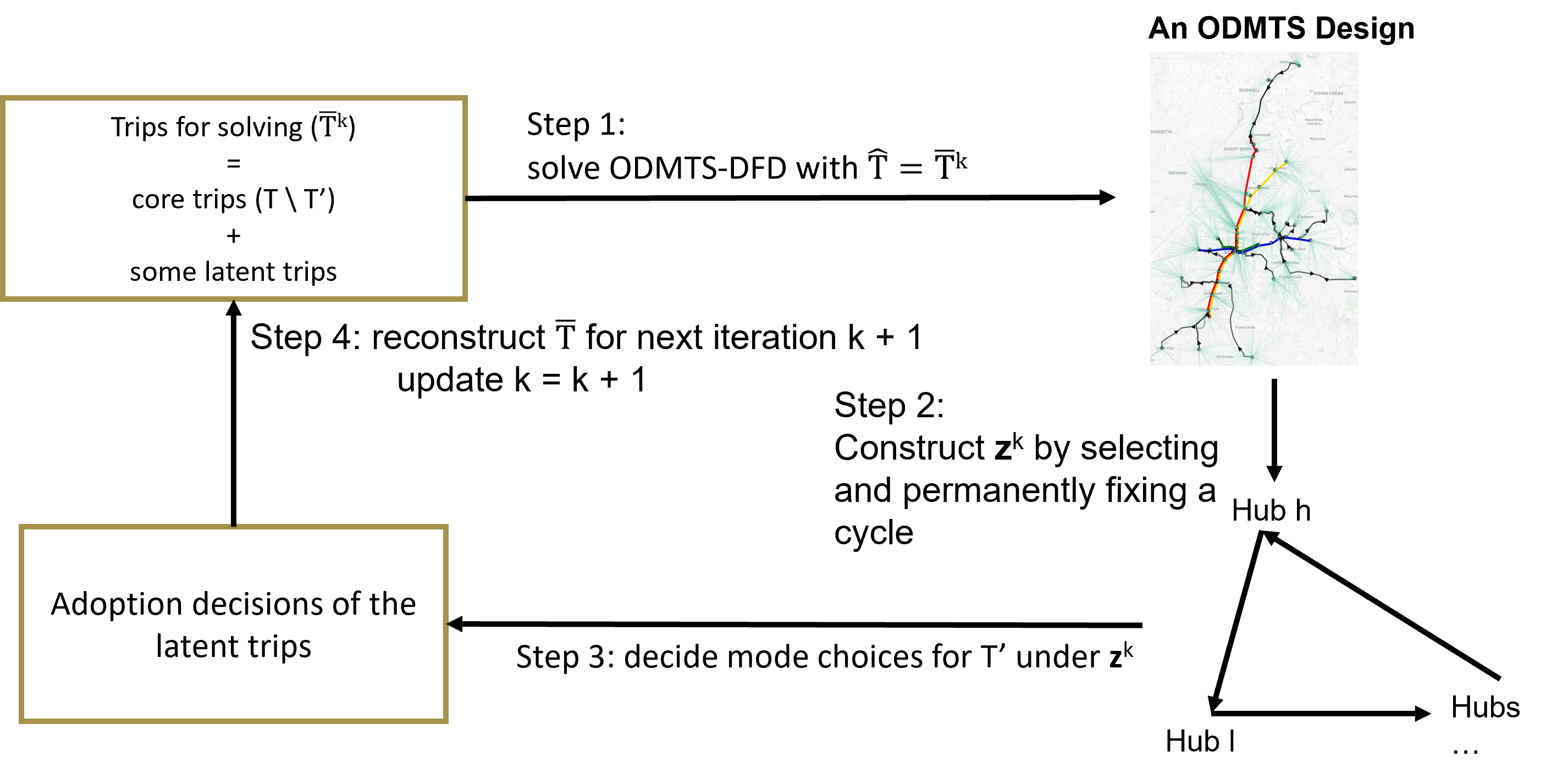
Figure 4: A Flowchart Describing an Iteration of Arc-Based Algorithms.

This section introduces the second type of iterative algorithms: arc based iterative algorithms. Figure 4 summarizes their key steps. At the beginning of each iteration, these algorithms solve the ODMTS-DFD problem and obtain a network design. They then select a cycle from the open arcs in $\mathbf{z}$, which is permanently added to the network design for subsequent iterations. Note that a cycle itself is also a network design since it is a vector from set $\{0,1\}^{|H|\times|H|}$ satisfying the weak connectivity constraint (3b). The input trip set considered for the ODMTS-DFD problem is then expanded, considering the adoption decisions of the riders. These steps are iterated until no improving cycle can be added to the design.

Contrary to the trip-based algorithms, arc-based algorithms start with a fixed ODMTS design (which is empty initially), denoted as $\mathbf{z}_{fixed}$, and adds a cycle in each iteration. Moreover, since they select the best cycle with respect to the overall objective until no improvement is found, arc-based algorithms produce a sequence of network designs whose evaluation are monotonically decreasing. As a result, they find primal solutions quickly, which is not guaranteed in trip-based algorithms. In summary, arc-based algorithms satisfy the following properties:

1. The design objective (computed by function ${eval}(\mathbf{z})$) monotonically decreases.

2. The ODMTS design $\mathbf{z}_{fixed}$ monotonically increases.

This paper proposes two arc-based algorithms. Section 4.3.1 presents the Arc-based Greedy Algorithm arc-S1, the main arc-based iterative algorithm. Section 4.3.2 presents the algorithm arc-S2 that extends arc-S1 to overcome a challenge faced by arc-S1. Both algorithms are parametrized by one or more functions that expand the set of riders at each iteration. Section 4.3.3 introduces several expansion rules to construct these Expand functions used by the algorithms.

4.3.1 Arc-based Greedy Algorithm (arc-S1)

Algorithm arc-S1 describes the arc-based greedy algorithm. It maintains an upper bound $B^{k}$ that represents the best design found up to iteration $k$. arc-S1 also uses a generalization of the ODMTS-DFD, where the second parameter represents the set of arcs that must be fixed to 1 in the ODMTS-DFD solution (line 4).

During each iteration, after solving such a generalized ODMTS-DFD, the resulting design $\textbf{z}_{temp}^{k}$ is decomposed into two parts: $\textbf{z}_{fixed}$ and $\textbf{z}_{unfixed}^{k}$ (line 5). The partial design $\textbf{z}_{fixed}$ denotes all the arcs which were constrained to be opened in the ODMTS-DFD, while $\textbf{z}^{k}_{unfixed}$ is the remaining assignment in $\textbf{z}_{temp}^{k}$. Given that $\textbf{z}_{temp}^{k}$, $\textbf{z}_{unfixed}^{k}$, and $\textbf{z}_{fixed}$ all satisfy constraint (5b), the algorithm of Johnson (1975) can be used to find the set $Y^{k}$ of directed cycles (line 6). Each iteration attempts to add a new cycle $\textbf{y}^{k}\in Y^{k}$ to the fixed design $\textbf{z}_{fixed}$. Algorithm arc-S1 does this greedily, adding the cycle $\textbf{y}^{k}$ which provides the greatest decrease in $B^{k}$ (lines 10–18). Therefore, the series $B^{0},\ldots,B^{k}$ decreases monotonically over time, while the design $\textbf{z}_{fixed}$ expands over time (line 19). Note that the computational time of each iteration decreases since the number of variables decreases. Algorithm arc-S1 also expands the trips to consider in the ODMTS-DFD (lines 21–22).

Algorithm 4 arc-S1

1:  Set $k=0$, $\mathbf{z}_{fixed}=\vec{0}$, $\overline{T}^{0}=T\setminus T^{\prime}$, $B^{0}=\infty$.

2:  Require: Expand function for increasing the set of riders considered.

3:  while True do

4:     Set $\mathbf{z}_{temp}^{k}$ = ODMTS-DFD($\overline{T}^{k}$,$\{(h,l)\mid{{z}_{fixed}}_{hl}=1\ \wedge\ h,l\in H\}$).

5:     Set $\mathbf{z}^{k}_{unfixed}=\mathbf{z}_{temp}^{k}-\mathbf{z}_{fixed}$.

6:     Set $Y^{k}$ to the set of all cycles in $\mathbf{z}^{k}_{unfixed}$.

7:     if $Y^{k}=\emptyset$ then

8:        break.

9:     end if

10:     for all $\mathbf{y}\in Y^{k}$ do

11:        Set $obj_{\mathbf{y}}={eval}(\mathbf{z}_{fixed}+\mathbf{y})$

12:     end for

13:     Set ${obj}^{k}=\min\limits_{\mathbf{y}\in Y^{k}}\{obj_{\mathbf{y}}\}$ and $\mathbf{y}^{k}=\argmin\limits_{\mathbf{y}\in Y^{k}}\{obj_{\mathbf{y}}\}$.

14:     if ${obj}^{k}<B^{k}$ then

15:        Set $B^{k+1}={obj}^{k}$.

16:     else

17:        break.

18:     end if

19:     Set $\mathbf{z}_{fixed}$ = $\mathbf{z}_{fixed}+\mathbf{y}^{k}$.

20:     Set $\mathbf{z}^{k}$ = $\mathbf{z}_{fixed}$

21:     Set ${T^{\prime}}_{next}^{k}$ = Expand($T^{\prime},\mathbf{z}^{k}$).

22:     Set $\overline{T}^{k+1}=\overline{T}^{k}\cup{T^{\prime}}_{next}^{k}$.

23:     Set $k=k+1$.

24:  end while

25:  return  $\textbf{z}^{k}$

The algorithm terminates when the design objective bound is not decreasing, i.e., $B^{k}=B^{k+1}$. This can happen for two reasons:

1. $Y^{k}$ is empty, i.e., there are no new bus cycles.

2. No cycle in $Y^{k}$ provides a better objective value.

4.3.2 Arc-based Extended Greedy Algorithm (arc-S2)

The Expand function used in Algorithm arc-S1 significantly affects its performance. Assume, for instance, that the size of core trip set $T\setminus T^{\prime}$ is substantially smaller than the size of latent trip set $T^{\prime}$, which is almost always the case in practice. If the set of trips in $\overline{T}^{k}$ is too large, the proposed design becomes convoluted, many cycles are generated, and few trips adopt the ODMTS since it contains many bus lines, which degrade the convenience of the riders. On the other hand, if the set $\overline{T}^{k}$ is too small, the algorithm may terminate prematurely with a poor solution.

Algorithm 5 arc-S2

1:  Set $k=0$, $\mathbf{z}_{fixed}=\vec{0}$, $\overline{T}^{0}=T\setminus T^{\prime}$, $B^{0}=\infty$, $p=1$

2:  Require: Expand_i functions for increasing the set of riders considered ($i=1,2$)

3:  while $p\leq 2$ do

4:     while True do

5:        Set $\mathbf{z}_{temp}^{k}$ = ODMTS-DFD($\overline{T}^{k}$,$\{(h,l)\mid{{z}_{fixed}}_{hl}=1\ \wedge\ h,l\in H\}$).

6:        Set $\mathbf{z}^{k}_{unfixed}=\mathbf{z}_{temp}^{k}-\mathbf{z}_{fixed}$.

7:        Set $Y^{k}$ to the set of all cycles in $\mathbf{z}^{k}_{unfixed}$.

8:        if $Y^{k}=\emptyset$ then

9:           break.

10:        end if

11:        for all $\mathbf{y}\in Y^{k}$ do

12:           Set $obj_{\mathbf{y}}={eval}(\mathbf{z}_{fixed}+\mathbf{y})$

13:        end for

14:        Set ${obj}^{k}=\min\limits_{\mathbf{y}\in Y^{k}}\{obj_{\mathbf{y}}\}$ and $\mathbf{y}^{k}=\argmin\limits_{\mathbf{y}\in Y^{k}}\{obj_{\mathbf{y}}\}$.

15:        if ${obj}^{k}<B^{k}$ then

16:           Set $B^{k+1}={obj}^{k}$.

17:        else

18:           break.

19:        end if

20:        Set $\mathbf{z}_{fixed}$ = $\mathbf{z}_{fixed}+\mathbf{y}^{k}$.

21:        Set $\mathbf{z}^{k}$ = $\mathbf{z}_{fixed}$

22:        Set ${T^{\prime}}_{next}^{k}$ = Expand_p($T^{\prime},\mathbf{z}^{k}$).

23:        Set $\overline{T}^{k+1}=\overline{T}^{k}\cup{T^{\prime}}_{next}^{k}$.

24:        Set $k=k+1$.

25:     end while

26:     Set $p=p+1$

27:  end while

28:  return  $\textbf{z}^{k}$

To overcome this difficulty, arc-S2 implements a two-stage extension of arc-S1 by using two Expand functions. Initially, arc-S2 expands the set of trips slowly until convergence using function Expand₁. Then arc-S2 enters a second phase where the trip set increases faster. Both phases implement arc-S1, except that the second stage starts with the fixed design and the set of trips produced by phase 1.

4.3.3 Trip Expansion

The arc-based algorithms have been tested with a number of expansion rules to construct the Expand functions. The first three are intuitive: the expansion at the step $k$ includes

1. all latent trips that adopt $\textbf{z}^{k}$ ;

2. all latent trips that adopt $\textbf{z}^{k}$ and are profitable for the transit agency ;

3. all latent trips that adopt $\textbf{z}^{k}$ and are not served by direct shuttle .

When using expansion rule (a), Algorithm arc-S1 satisfies the following property.

Proposition 4

The ODMTS design returned of Algorithm arc-S1 with expansion rule (a) satisfies the correct rejection property (Property 1).

Proof.

Proof: When Algorithm arc-S1 terminates at iteration $k$, the design $\mathbf{z}_{fixed}$ does not change. That means that the ODMTS-DFD was executed with $\hat{T}^{k}=\overline{T}^{k-1}\cup{T^{\prime}}_{next}^{k-1}$. Moreover, ${T^{\prime}}_{next}^{k-1}$ is the set of all latent trips that adopt $\mathbf{z}_{fixed}$. Hence, all latent trips that are not in $\hat{T}^{k}$ reject design $\mathbf{z}^{k}$ and Property 1 holds. ∎

This result extends to Algorithm arc-S2.

Corollary 2

The ODMTS design returned by algorithm arc-S2 with expansion rule (a) in the second stage satisfies the correct rejection property (Property 1).

The rest of this section presents an additional rule that exploits properties of trip durations and choice functions. It relies on the following proposition by Basciftci and Van Hentenryck (2022).

Proposition 5

Consider an ODMTS design $\mathbf{z}^{1}$, and any ODMTS design $\mathbf{z}^{2}\geq\mathbf{z}^{1}$. Let the ODMTS travel time for trip $r$ under $\mathbf{z}^{1}$ and $\mathbf{z}^{2}$ be denoted as $t^{1}$ and $t^{2}$. Then $t^{2}$ is bounded by an upper bound $UB^{r}$ defined as follows:

$$UB^{r}=\begin{cases}t^{1}+\frac{(1-\theta)}{\theta}g\left(d_{or^{r}m}+d_{nde^{r}}-\min\limits_{h,l\in H}\left\{d_{or^{r}h}+d_{lde^{r}}\right\}\right),\\ \text{if trip $r$ is assigned to a multimodal route under design $\mathbf{z}^{1}$ such that}\\ \text{$m$ and $n$ are the first and last hub in the route, respectively}\\ \\ \max\left\{t^{1},t^{1}+\frac{(1-\theta)}{\theta}g\left(d_{or^{r}de^{r}}-\min\limits_{h,l\in H}\left\{d_{or^{r}h}+d_{lde^{r}}\right\}\right)\right\},\\ \text{if trip $r$ is assigned to a direct shuttle route under design $\mathbf{z}^{1}$}\\ \end{cases}$$

This result has an important consequence: if trip $r$ adopts the transit system under $\mathbf{z}^{1}$ and $UB^{r}\leq\alpha^{r}t^{r}_{cur}$, then trip $r$ also adopts the ODMTS under any design $\mathbf{z}^{2}$ with $\mathbf{z}^{2}\geq\mathbf{z}^{1}$. Since the ODMTS designs of the arc-based algorithms monotonically increase over time, every adopting trip $r$ satisfying $UB^{r}\leq\alpha^{r}t_{cur}^{r}$ at some iteration $k$ is guaranteed to adopt the ODMTS design in any subsequent iteration $l>k$. These results suggest an interesting expansion rule:

1. include every latent trip $r$ that adopts $\textbf{z}^{k}$ and satisfies $UB^{r}\leq\alpha^{r}t_{cur}^{r}$.

Algorithm arc-S1 with expansion rule (d) satisfies the following property.

Proposition 6

The ODMTS design found by Algorithm arc-S1 with expansion rule (d) satisfies the correct adoption property (Property 2).

Proof.

Proof: Consider the series of designs $\mathbf{z}^{0},\mathbf{z}^{1}...,\mathbf{z}^{k}$ found by Algorithm arc-S1 using expansion rule (d); we have $\mathbf{z}^{0}\leq\mathbf{z}^{1}\leq...\leq\mathbf{z}^{k}$ by construction. Moreover, $\mathbf{z}^{0}$ satisfies the correct adoption property since there are no latent trips included in $\hat{T}=\overline{T}^{0}$. For an arbitrary design $\mathbf{z}^{i}$ where $0<i\leq k$, it follows that all latent trips included in $\hat{T}=\overline{T}^{i}=(T\setminus T^{\prime})\cup\bigg{(}\bigcup\limits_{j=0,...,i-1}T^{\prime j}_{next}\bigg{)}$ adopt $\mathbf{z}^{i}$ by definition of expansion rule (d) and because trips in $T^{\prime j}_{next}$ for any $j=0,1,...,i-1$ adopt $\mathbf{z}^{i}$, which is greater than any $\mathbf{z}^{j}$. Thus, all of these designs satisfy the correct adoption property. ∎

Additionally, when applying Algorithm arc-S2 in practice, it is worth noticing that the first rule should not be rule (a) since trips satisfying rule (b), (c), and (d) also satisfy rule (a).

5 Computational Study with a Regular-sized Dataset

This section presents a case study using a realistic dataset from AAATA (https://www.theride.org Last Visited Date: July 27th, 2022), the transit agency serving Ypsilanti and the broader of Ann Arbor region of Michigan, USA. Since the exact algorithm introduced by Basciftci and Van Hentenryck (2022) can successfully find the optimal design in a reasonable amount of time on this regular-sized dataset, this case study aims at demonstrating the workability of the iterative algorithms proposed in Section 4 by comparing computational results obtained from the iterative algorithms and the exact algorithm. Section 5.1 introduces the experimental setting, and Section 5.2 shows the results found by the iterative algorithms under four different configurations.

5.1 Experimental Setting

Figure 5: The 1267 bus stops used in this case study. The enlarged 10 stops are the designated hubs. The low-income, middle-income, and high-income stops are represented by red circles, grey squares, and blue triangles respectively.

This case study is based on the AAATA transit system that operates over 1,267 stops. In order to design an ODMTS, 10 stops are designated as ODMTS hubs, and the other stops are only accessible to on-demand shuttles. There are 1,503 trips for a total of 5,792 riders, and each trip is represented by an origin stop and a destination stop. The time horizon for this case study is between 6pm and 10pm. Therefore, this dataset primarily consists of commuting trips from work locations to home.

The mode preference of a rider depends on her income level, i.e, a rider with higher income level has lower tolerance on the amount of ODMTS travel time. The whole 1,503 trips were first divided into three different categories: low-income, middle-income, and high-income. The classification of income level is solely decided by a trip’s destination because it is approximately a rider’s home location. Figure 5 visualizes the locations of the stops and their corresponding income levels. If a trip is assigned to a certain income-level class, all riders belong to this trip are then assumed to have the same income-level. Following this procedure, there are 476 low-income, 819 middle-income, and 208 high-income trips with 1,754, 3,316, and 722 riders respectively. Once the classification is carried out, an $\alpha$ value associated to Equation (2) is assigned to each class. It must be noted that all trips in the low-income class are treated as members of the core trips set $T\setminus T^{\prime}$; hence, no $\alpha$ value is required for them. For the middle-income and the high-income classes, 2.0 and 1.5 are employed as the $\alpha$ values, respectively.

In order to evaluate the performances of all five iterative algorithms with different configurations, two values for each of the two parameters—rider multiplier and core trips percentage are selected, resulting in overall four experiments as described in Table 1. More specifically, the rider multiplier parameter multiplies the number of riders for each trip. The core trips percentage parameter is utilized to divide the dataset into core trips and latent trips by varied partitions.

The on-demand shuttle price is fixed at $1 per kilometer and each shuttle is assumed to only serve one passenger. Shuttles between bus hubs are not allowed in this case study. For buses, the operating fee is $3.87 per kilometer. Four buses per hour is the unique bus frequency considered here; hence, each opened bus leg has an average waiting time ($t_{hl}^{wait}$ in (4c) and (6c)) of 7.5 minutes. For passengers, there is no limit on the number of transfers. A constant ticket price that is consistent with the existing AAATA system is applied. Thus, a full ODMTS service charges $2.5 for each individual regardless of the travel length. Inconvenience is measured in seconds, and the inconvenience and cost parameter $\theta$ is fixed at 0.001.

The iterative algorithms and the exact algorithm are programmed with Python 3.7. The exact algorithm is set to terminate if it reaches a 0.1% optimality gap; otherwise, it reports the upper bound as the “optimal” solution after a 6 hour time limit. The computational experiments are carried out using Gurobi 9.5 as the solver without multi-threading techniques applied to the sub-problems in ODMTS-DFD (Figure 1). For the trip-based iterative algorithms, the $\rho$ value for Algorithm LABEL:rho_GRAD and Algorithm LABEL:rho_GAGR, and the $\eta$ value for Algorithms LABEL:alg:m_GRRE and LABEL:rho_GAGR are both set to 10. For arc-based iterative algorithms, two experimental runs are designed to test Algorithm arc-S1 with trip expansion rules (a) and (d). Algorithm arc-S2 employs rules (c) and (a) and rules (d) and (a) for the two stages. When solving the ODMTS-DFD problem at each iteration, all iterative algorithms employ a stand-alone ODMTS solving tool developed by Dalmeijer and Van Hentenryck (2020) that leverages Benders decomposition algorithm. This tool is based on the solver CPLEX 12.9 and allows multi-threading when solving sub-problems in ODMTS-DFD. However, in this case study, multi-threading techniques are disabled in order to fairly compare the algorithmic performances.

	ridership	low income core trips			medium income core trips			high income core trips
		% trips	# trips	# riders	% trips	# trips	# riders	% trips	# trips	# riders
Exp.1	regular	100%	476	1754	75%	614	2842	50%	104	434
Exp.2	regular	100%	476	1754	50%	409	2262	25%	52	258
Exp.3	doubled	100%	476	3508	75%	614	5684	50%	104	868
Exp.4	doubled	100%	476	3508	50%	409	4524	25%	52	516

Table 1: The experimental setups for the four experiments. For doubled ridership, the number of riders for each O-D pair is multiplied by 2. The core trips percentages for each income level are [100%, 75%, 50%] and [100%, 50%, 25%] for low, medium, and high income trips, respectively.

5.2 Evaluation of the ODMTS Designs

This section evaluates ODMTS designs found by the exact algorithm and the iterative algorithms. To compute False Rejection Rate ($\%R_{false}$) and False Adoption Rate ($\%A_{false}$) under the optimal design $\mathbf{z}^{*}$ of the exact algorithm, the trip set $\hat{T}^{*}$ is constructed with $(T\setminus T^{\prime})\cup\{r\in T^{\prime}:(\delta^{r})^{*}=1\}$ as discussed in Proposition 1. For iterative algorithms, remember that Algorithms LABEL:alg:m_GRRE and LABEL:rho_GAGR report the design with the minimal objective. That is, an intermediate design found by these algorithms might be reported in this section. Furthermore, note that, although only a subset of trips is used to obtain the design in all algorithms, the design evaluation is computed with all core trips and latent trips.

6 Large-Scale Case Study

This section presents another real case study conducted with travel data representing a regular workday in Atlanta, Georgia, to evaluate the performance of the iterative algorithms on large-scale instances. This case study focuses on the 6am–10am morning peak of a regular weekday, and the ODMTS operates over 2,426 stops with 66 designated hubs. Among the 66 hubs, 38 of them are adopted from MARTA rail stations. There are 15,478 core trips, 36,283 latent trips with 55,871 existing riders, and 54,902 riders with choices. Appendix 8 introduces the data and its generation process in detail. After the experimental setting is explained in Section 6.1, Section 6.2 presents the computational results and demonstrates the advantages of the iterative algorithms for the ODMTS Design with Adoptions problem.

6.1 Experimental Setting

The MARTA rail system, which is the rail system of the Atlanta Metropolitan area, is completely preserved in this experiment and the passenger travel time between any two rail stations are derived from GTFS data. Therefore, the decision variables ${z}_{hl}\>\forall h,l\in\{\text{rail hubs}\}$ are fixed at 1 when solving the ODMTS-DA (Figure 1) and the ODMTS-DFD (Figure 2). The unique bus frequency considered in this experiment is six buses per hour; hence, the average waiting time ($t_{hl}^{wait}$ in (4c) and (6c)) for an ODMTS bus is five minutes. Shuttles are allowed to move between hubs in this case study. Additionally, bus arcs are not allowed to overlap rail arcs and, for each hub, a bus arc can only be placed between the hub itself and its closest ten hubs in terms of travel time to simplify the problem setting. For the adoption equation (2), $\alpha=1.5$ is applied to all latent trips.

A $2.5 ticket is charged for each ODMTS rider and this constant price is identical to the current service provided by MARTA. The operating price for on-demand shuttle and buses are fixed at $0.62 per km ($1 per mile) and $72.15 per hour, respectively. The inconvenience and cost parameter $\theta$ is fixed at $7.25/(60+7.25)$. This case study employs minute as the unit of time in computation. These parameter values are directly adopted from an Atlanta-based ODMTS study presented in Auad et al. (2021).

For the exact algorithm, the running time is limited at 24 hours. Due to the complexity of the master problem in the ODMTS-DA problem (Figure 1), for each iteration of the exact algorithm, the master problem terminates when reaching to 1% MIP gap or an 8 hours time limit. For the trip-based iterative algorithms, the iterative step sizes $\rho$ and $\eta$ are tested with three values—1000, 2000, and 3000. The step size that leads to the best design objective is reported together with the best discovered ODMTS design. In particular, Algorithm LABEL:rho_GRAD and Algorithm LABEL:alg:m_GRRE only demand the $\rho$ value and the $\eta$ value respectively, and $\eta$ is set to equal to $\rho$ for Algorithm LABEL:rho_GAGR. The combined trip-based iterative algorithm, i.e., Algorithm LABEL:rho_GAGR, is also terminated after 24 hours of running time. For the arc-based iterative algorithms, expansion rule (a) and (d) are separately utilized by Algorithm arc-S1. The two-stage Algorithm arc-S2 employs two groups of rules—(i) rules (c) and (a) and (ii) rules (d) and (a). Furthermore, at the starting point, $\mathbf{z}_{fixed}$ represents the MARTA rail system. Lastly, the same set of computational tools and solvers are used as in Section 5.1.

6.2 Computational Results

This section evaluates the computational results of the large-scale case study from various viewpoints. First, Section LABEL:subsubsect:atl_obj_eval compares the design objectives found by the exact algorithm and the iterative algorithms. It also discusses the False Rejection Rates and False Adoption Rates of the algorithms. Section LABEL:subsubsect:atl_design_adoption_results then presents the ODMTS designs and the adoption status. Section LABEL:subsubsect:atl_other_results analyzes the ODMTS designs using multiple performance measures including travel time, travel distance, and operating cost.

7 Conclusion

This study aimed at capturing the latent demand for the transit agency such that the transit services can concurrently provide high-quality services to existing riders and extend the services to current under-served areas. Prior work proposed a bilevel optimization formulation (Figure 1), referred to as the ODMTS Design with Adoption problem (ODMTS-DA) in this paper, which was solved by an exact algorithm. However, due to the complexity of the proposed problem, applying the exact algorithm on large-scale instances remains computationally challenging.

This paper attempted to address this limitation and proposed five heuristic algorithms to efficiently approximate the optimal solution of the ODMTS-DA problem. The fundamental idea of these iterative algorithms is to separate the previous bilevel framework into two individual but simpler components, i.e., a regular ODMTS problem with no adoption awareness (the ODMTS-DFD problem in Figure 2) and an evaluation procedure based on a mode choice function (e.g., Equation (2)). These heuristic algorithms can be further categorized into two general classes based on their algorithmic designs: (1) trip-based algorithms and (2) arc-based algorithms. In general, at each iteration, the trip-based algorithms reconstruct the trip sets for the regular ODMTS problem and the arc-based algorithms attempt to fix a certain amount of bus arcs. The advantages and limitations of each algorithm are discussed in this paper, and several theoretical properties are derived from the optimal solutions in order to provide more guidelines for the iterative algorithms under varied circumstances. In particular, two key properties, i.e., correct rejection (Property 1) and correct adoption (Property 2), are introduced. The false rejection rate and the false adoption rate are used as metrics to evaluate the ODMTS designs, providing additional insights on the performance of the heuristic algorithms when an an optimal solution becomes unavailable for large-scale instances.

This paper also present two comprehensive case studies to validate the heuristic algorithms. The first case study is carried out with a normal-sized transit dataset collected by the transit agency in the Ann Arbor and Ypsilanti area in the state of Michigan. The results demonstrate that the heuristic algorithms can discover the optimal ODMTS design. The second case study is based on multi-sourced data and includes a very large numbers of stops and trips. The main goal of this case study is to show the advantages of the heuristic algorithms on large-scale instances. Compared to the exact algorithm, the heuristic algorithms achieve better objective values in considerably less amount of time. Moreover, the obtained ODMTS designs are superior in terms of travelled distance by cars, operating cost, and travel convenience for the transit agencies. Future research directions include the design and evaluation of complex choice models and the integration of demographic data.

8 Data Generation for Large-Scale Case Study

This section first introduces the procedures to construct the core demand and latent demand used in the large-scale case study. It then describes the process of allocating a set of ODMTS stops with high granularity.

8.1 Core Demand

This core demand of this case study is based on two realistic datasets provided by the transit agency Metropolitan Atlanta Rapid Transit Authority (MARTA). One dataset includes the transit pass transaction records collected by the Automated Fare Collection (AFC) system, and the other dataset is constructed using Automated Passenger Counter (APC) system in the MARTA buses. These two dataset are combined to generate a set of trips that represent a regular weekday in March 2018. For practical reasons, all MARTA stops within a $1500\text{\,}\mathrm{f}\mathrm{e}\mathrm{e}\mathrm{t}$ ($457.2\text{\,}\mathrm{m}$) radius are first clustered into 1,585 cluster stops. The core trip set $T\setminus T^{\prime}$ is then constructed after narrowing the time window to the morning peak and applying trip chaining techniques, and they are identical to the data employed by Auad et al. (2021) for the baseline scenarios.

8.2 Latent Demand

This section introduces the source of the latent demand for this case study. The ABM-ARC dataset is simulated by the Atlanta Regional Commission (ARC) based on the ARC Regional Household Travel Survey conducted in 2011 following a rigorous traditional four-step activity-based model (ABM) (http://abmfiles.atlantaregional.com/ Last Visited Date: November 24th, 2021). In this dataset, there are more than 4.5 million simulated agents who are characterized by demographic data corresponding to themselves and their households. It also contains more than 13 million individual tours that are completed in the Atlanta metropolitan area in a typical weekday. All tours are described by detailed travel information including origin-destination (O-D) locations, travel period, travel distance, travel mode, and purposes. In particular, the data with horizon year 2020 is used for this case study to align with the 2018 core demand.

The latent demand for this case study consists of all individual tours that satisfy the following five conditions: (i) drive alone tours, (ii) commuting tours, (iii) the tours start between 6am and 10am, (iv) tour agents whose households are located inside the East Atlanta region—a large and generally undeserved residential area, and (v) tour agents whose work locations located inside or around the I-285 interstate highway loop or inside the city of Sandy Springs—both are MARTA’s primary service regions. The first two conditions regulate tour mode and tour purposes such that commuters who drive alone form the potential market of an ODMTS service. Particularly, the second condition regulates tour purpose because a commuter’s household and work location are not regularly changed; hence, these tours are more representative of a regular weekday. The third condition further refines the dataset by narrowing down the time window to the morning peak. The last two conditions control the origin and destination locations. It is worth pointing out that this study keeps the tour destination rather than the first trip-leg destination in order to generalize the home-to-work demand for people reside in East Atlanta. Once the valid tours are isolated from the ABM-ARC dataset, their tour origins and tour destinations are then extracted to form the latent demand for this case study.

All the geographical information in the ABM-ARC dataset are at Traffic Analysis Zone (TAZ) level; however, instead of directly utilizing the TAZ centroids to represent the exact locations, origins and destinations are further sampled to lower geographical levels to construct a more representative dataset. In particular, a TAZ can be decomposed into multiple Census Blocks that belong to or intersect with it. A Census Block consists of one or several adjacent neighbourhoods and records the number of residents. Since all selected trips originate from the commuters’ home locations, each origin is sampled from its corresponding TAZ to a Census Block by the population distribution of the census blocks. Similarly, the destinations are sampled from TAZ level to Points of Interest (POI) level. Points of interest are specific locations such as restaurants, schools, and factories. POIs are associated with a TAZ and their area size is also recorded; thus, in this study, each destination is sampled from its corresponding TAZ to a POI by the area distribution of the POIs.

8.3 ODMTS Stops, O-D Pairs, and Hubs

(a) ODMTS stops

(b) ODMTS Hubs

(c) MARTA Rail Lines

Figure 6: The 2,426 ODMTS stops are shown in (a). The blue circles, red triangles, and yellow triangles denote the locations of the MARTA cluster stops, stops adopted from Census Block centers, and stops adopted from Points of Interest centers, respectively. The 66 ODMTS hubs and the MARTA rail system are visualized in (b) and (c) respectively. All 38 MARTA rail stations are reserved as ODMTS hubs.

(a) O-Ds in Core Trip Set $T\setminus T^{\prime}$

(b) O-Ds in Latent Trip Set $T^{\prime}$

Figure 7: The heat-maps in (a) visualize the origin stops and destination stops of the core trip set $T\setminus T^{\prime}$. All origins and destinations are MARTA cluster stops. The heat-maps in (b) visualize the origin stops and destination stops of the Latent Trip set $T^{\prime}$. All origins are from the East Atlanta area, and all destinations are either inside or around the I-285 interstate or inside the city of Sandy Springs. The origins and destinations are first sampled to lower geographical level, then mapped to its nearest ODMTS stops.

The 2,426 ODMTS stops are allocated on the basis of three sources: (i) the 1,585 MARTA cluster stops, (ii) the centers of Census Blocks in East Atlanta, (iii) the centers of POIs inside or around the I-285 interstate highway loop or inside the city of Sandy Springs. Specifically, all 1,585 MARTA cluster stops are first reserved as the ODMTS stops. To improve the granularity of stops such that the maximum straight-line distance between a stop and its nearest stop is $457.2\text{\,}\mathrm{m}$ ($1500\text{\,}\mathrm{f}\mathrm{e}\mathrm{e}\mathrm{t}$), 247 Census Block centers and 594 POI centers are then appointed as the ODMTS stops. The ODMTS stops are illustrated in Figure 6(a). The car travel time and car travel distance are queried from database constructed in accordance with OpenStreetMap (https://planet.osm.org/ Last Visited Date: July 24th, 2022). It should be pointed out that traffic congestion is not taken into account due to the limited access to OpenStreetMap. However, shuttle legs are usually short and local; thus, shuttle operations are less affected by congestion.

Following the allocation of ODMTS stops, for each trip in the latent demand, its origin and destination are mapped to their nearest ODMTS stops with regards to straight-line distance. At this stage, the Latent Trip set $T^{\prime}$ is constructed. It should be recalled that the trips in the core trip set $T\setminus T^{\prime}$ originate from and arrive at MARTA cluster stops, which are already ODMTS stops. The origin stops and destination stops of the core trip set $T\setminus T^{\prime}$ and Latent Trip set $T^{\prime}$ are illustrated as heat-maps in Figure 7(a) and Figure 7(b), respectively.

As shown in Figure 6(b), 66 ODMTS stops are designated as ODMTS hubs. Among these hubs, 38 of them are MARTA rail stations and the rail system is illustrated in 6(c). The other 28 stops are appointed as hubs following these four rules: (1) the stops are on major roads, (2) there are a considerable amount of riders who depart from or arrive at this stop, (3) the straight-line distance between two hubs are at least $1\text{\,}\mathrm{k}\mathrm{m}$, and (4) a particular emphasis on the East Atlanta region should be shown.

References

- Alumur, Kara, and Karasan (2012) Alumur SA, Kara BY, Karasan OE, 2012 Multimodal hub location and hub network design. Omega 40(6):927–939.
- Auad et al. (2021) Auad R, Dalmeijer K, Riley C, Santanam T, Trasatti A, Van Hentenryck P, Zhang H, 2021 Resiliency of on-demand multimodal transit systems during a pandemic. Transportation Research Part C: Emerging Technologies 133.
- Basciftci and Van Hentenryck (2020) Basciftci B, Van Hentenryck P, 2020 Bilevel optimization for on-demand multimodal transit systems. Hebrard E, Musliu N, eds., Integration of Constraint Programming, Artificial Intelligence, and Operations Research, 52–68 (Springer International Publishing).
- Basciftci and Van Hentenryck (2022) Basciftci B, Van Hentenryck P, 2022 Capturing travel mode adoption in designing on-demand multimodal transit systems. Transportation Science URL https://pubsonline.informs.org/doi/full/10.1287/trsc.2022.1184.
- Canca et al. (2016) Canca D, De-Los-Santos A, Laporte G, Mesa JA, 2016 A general rapid network design, line planning and fleet investment integrated model. Annals of Operations Research 246(1):127–144.
- Canca et al. (2017) Canca D, De-Los-Santos A, Laporte G, Mesa JA, 2017 An adaptive neighborhood search metaheuristic for the integrated railway rapid transit network design and line planning problem. Computers & Operations Research 78:1–14.
- Canca et al. (2019) Canca D, De-Los-Santos A, Laporte G, Mesa JA, 2019 Integrated railway rapid transit network design and line planning problem with maximum profit. Transportation Research Part E: Logistics and Transportation Review 127:1–30.
- Cipriani, Gori, and Petrelli (2012) Cipriani E, Gori S, Petrelli M, 2012 Transit network design: A procedure and an application to a large urban area. Transportation Research Part C: Emerging Technologies 20(1):3–14.
- Dai et al. (2019) Dai W, Zhang J, Sun X, Wandelt S, 2019 Hubbi: Iterative network design for incomplete hub location problems. Computers & Operations Research 104:394–414.
- Dalmeijer and Van Hentenryck (2020) Dalmeijer K, Van Hentenryck P, 2020 Transfer-expanded graphs for on-demand multimodal transit systems. International Conference on Integration of Constraint Programming, Artificial Intelligence, and Operations Research, 167–175 (Springer).
- Dumas, Aithnard, and Soumis (2009) Dumas J, Aithnard F, Soumis F, 2009 Improving the objective function of the fleet assignment problem. Transportation Research Part B: Methodological 43(4):466–475.
- Fan and Machemehl (2006) Fan W, Machemehl RB, 2006 Optimal transit route network design problem with variable transit demand: genetic algorithm approach. Journal of transportation engineering 132(1):40–51.
- Gattermann, Schiewe, and Schöbel (2016) Gattermann P, Schiewe A, Schöbel A, 2016 An iterative approach for integrated planning in public transportation. 9th Triennial Symposium on Transportation Analysis.
- Hartleb et al. (2021) Hartleb J, Schmidt M, Huisman D, Friedrich M, 2021 Modeling and solving line planning with integrated mode choice URL http://dx.doi.org/10.2139/ssrn.3849985.
- Johnson (1975) Johnson DB, 1975 Finding all the elementary circuits of a directed graph. SIAM Journal on Computing 4(1):77–84.
- Klier and Haase (2008) Klier MJ, Haase K, 2008 Line optimization in public transport systems. Operations Research Proceedings 2007, 473–478 (Springer).
- Klier and Haase (2015) Klier MJ, Haase K, 2015 Urban public transit network optimization with flexible demand. Or Spectrum 37(1):195–215.
- Kroon, Maróti, and Nielsen (2015) Kroon L, Maróti G, Nielsen L, 2015 Rescheduling of railway rolling stock with dynamic passenger flows. Transportation Science 49(2):165–184.
- Lee and Vuchic (2005) Lee YJ, Vuchic VR, 2005 Transit network design with variable demand. Journal of Transportation Engineering 131(1):1–10.
- Liu et al. (2019) Liu D, Vansteenwegen P, Lu G, Peng Q, 2019 An iterative approach for profit-oriented railway line planning. Linköping University Electronic Press 806–825.
- Liu et al. (2021) Liu J, Chen W, Yang J, Xiong H, Chen C, 2021 Iterative prediction-and-optimization for e-logistics distribution network design. INFORMS Journal on Computing .
- Lodi et al. (2016) Lodi A, Malaguti E, Stier-Moses NE, Bonino T, 2016 Design and control of public-service contracts and an application to public transportation systems. Management Science 62(4):1165–1187.
- Mahéo, Kilby, and Van Hentenryck (2019) Mahéo A, Kilby P, Van Hentenryck P, 2019 Benders decomposition for the design of a hub and shuttle public transit system. Transportation Science 53(1):77–88.
- Schöbel (2012) Schöbel A, 2012 Line planning in public transportation: models and methods. OR spectrum 34(3):491–510.
- Schöbel (2017) Schöbel A, 2017 An eigenmodel for iterative line planning, timetabling and vehicle scheduling in public transportation. Transportation Research Part C: Emerging Technologies 74:348–365.
- Sutlive and Tomlinson (2019) Sutlive C, Tomlinson CS, 2019 2019 annual report and audit: Planning for the forward motion of metro atlanta. https://atltransit.ga.gov/wp-content/uploads/2019/12/ATL_ARA-Final-11-25-19.pdf.
- Tawfik, Gendron, and Limbourg (2021) Tawfik C, Gendron B, Limbourg S, 2021 An iterative two-stage heuristic algorithm for a bilevel service network design and pricing model. European Journal of Operational Research .
- Tawfik and Limbourg (2019) Tawfik C, Limbourg S, 2019 A bilevel model for network design and pricing based on a level-of-service assessment. Transportation Science 53(6):1609–1626.
- Yu, Yang, and Yao (2010) Yu B, Yang Z, Yao J, 2010 Genetic algorithm for bus frequency optimization. Journal of Transportation Engineering 136(6):576–583.