Effective good divisibility of rational homogeneous varieties

Abstract.

We compute the effective good divisibility of a rational homogeneous variety, extending an earlier result for complex Grassmannians by Naldi and Occhetta. Non-existence of nonconstant morphisms to rational homogeneous varieties of classical Lie type are obtained as applications.

1. Introduction

The notion of effective good divisibility $\mbox{e.d.}(X)$ of a complex projective manifold $X$ was introduced by Muñoz, Occhetta and Solá Conde [16], refining the notion of good divisibility introduced by Pan [19]. It is the upper bound of the total degree $i+j$ of two nonzero effective classes $x_{i}\in H^{2i}(X)$ and $x_{j}\in H^{2j}(X)$ with $x_{i}\cup x_{j}\neq 0$. It has nice applications on the nonexistence of nonconstant morphisms. As shown by Naldi and Occhetta [18], the effective good divisibility of a complex Grassmannian $Gr(m,n+1)$ is equal to $n+1$. It is then quite natural to ask for this quantity for a general rational homogeneous variety $G/P$, the quotient of a complex simple and simply-connected Lie group $G$ by its parabolic subgroup $P$.

The question on $\mbox{e.d.}(G/P)$ is actually closely related with a problem of characterizing the degree of quantum variables in quantum product, in earlier and extensive studies of quantum cohomology. The quantum cohomology ring $QH^{*}(G/P)=(H^{*}(G/P)\otimes\mathbb{Z}[\mathbf{q}],\star)$ is a deformation of the classical cohomology $H^{*}(G/P)$, by incorporating genus zero, three-pointed Gromov-Witten invariants. It has a canonical basis of Schubert classes $[X_{u}]$, and the evaluation $[X_{u}]\star[X_{v}]|_{\mathbf{q}=\mathbf{0}}$ coincides with $[X_{u}]\cup[X_{v}]$. As shown in [12], the quantum product $[X_{u}]\star[X_{v}]$ never vanishes, leading to the characterization of the degree of $\mathbf{q}$ and particularly the minimal degree $\mathbf{d}_{\rm min}$ in such individual product asked two decades ago. The characterization was provided for complex Grassmannians therein, for (co)minuscule Grassmannians in [8, 6] and for Grassmannians of types B and C in [23]. There has also been extended study in the context of quantum $K$-theory [4, 3]. With this terminology, $\mbox{e.d.}(G/P)$ is equivalent to the upper bound of the total degree of all Schubert classes $[X_{u}]$ and $[X_{v}]$ that satisfy $\mathbf{d}_{\rm min}=0$ in $[X_{u}]\star[X_{v}]$. As we will see, the viewpoint from quantum cohomology is particularly useful in the study of $\mbox{e.d.}(G/P)$ in the case of minuscule Grassmannians of classical Lie type.

Let $\mathcal{D}$ denote the Dynkin diagram of $G$ with the set $\Delta$ of nodes, for which we take the same numbering as on page 58 of [15]. Parabolic subgroups $P$ of $G$ that contain a fixed Borel subgroup $B$ are in one-to-one correspondence with the subsets $\Delta_{P}$ of $\Delta$. Let $P_{m}$ be the maximal parabolic subgroup that corresponds to the subset $\Delta\setminus\{\alpha_{m}\}$. By $\mathcal{D}(m)$ we mean the Grassmannian $G/P_{m}$ with $G$ being of type $\mathcal{D}$. Then $\mbox{A}_{n}(m)$ is the complex Grassmannian $Gr(m,n+1)$, and $\mathcal{D}_{m}$ can be realized as isotropic Grassmannians for other classical types. As a first main result, we obtain the following, where the known cases $\mbox{A}_{n}(m)$ and $G_{2}(m)$ are included for completeness.

Theorem 1.1.

The effective good divisibility $\mbox{e.d.}(\mathcal{D}(m))$ is given in Table 1.

Table 1. Effective good divisibility e.d. of $\mathcal{D}(m)$

$\mathcal{D}$				$\mbox{D}_{n+1}(m)$		$\mbox{F}_{4}$
$m$	$\mbox{A}_{n}(m)$	$\mbox{B}_{n}(m)$	$\mbox{C}_{n}(m)$	$1,n,n+1$	$2\leq m<n$	$1,4$	$2,3$	$\mbox{G}_{2}(m)$
e.d.	$n$	$2n-1$	$2n-1$	$2n-1$	$2n$	$12$	$14$	$5$

$\mathcal{D}$	$\mbox{E}_{6}$			$\mbox{E}_{7}$					$\mbox{E}_{8}$
$m$	$1,6$	$2,3,5$	4	1	2,6	3	4,5	7	1	$2,3,5$	4	6	7	8
e.d.	12	14	15	22	23	24	25	19	46	50	51	48	45	40

The above theorem will be proved for classical types in section 3.4 and for exceptional types in section 4. As from Table 1, the effective good divisibility of Grassmannians $G/P_{m}$ may equal each other for distinct $m$. For instance, $\mbox{e.d.}(\mbox{E}_{7}(2))=\mbox{e.d.}(\mbox{E}_{7}(6))=23$; $\mbox{e.d.}(\mathcal{D}(m))$ is independent of $m$, whenever $\mathcal{D}$ is of type A, B, C or $\mbox{G}_{2}$.

The nonvanishing of $[X_{u}]\cup[X_{v}]$ in $H^{*}(G/P)$ is equivalent to the nonempty intersection of Schubert variety $X_{u}$ and another Schubert variety $X^{v^{\sharp}}$ opposite to $X_{v}$. This is further equivalent to the property $u\leq v^{\sharp}$ with respect to the Bruhat order. Then we can reduce it to the Bruhat order among Grassmannian permutations. Such reduction is well known for type Lie A (see for instance [10, exercise 8 on page 175]). The reduction for general Lie type should have also been known to the experts, while we treat it as a special case of [4, Theorem 5], for not being aware of a precise reference elsewhere. As a consequence, we obtain the following.

Theorem 1.2.

The effective good divisibility of $G/P$ of any type $\mathcal{D}$ is given by

$$\mbox{e.d.}(G/P)=\min\{\mbox{e.d.}(\mathcal{D}(m))\mid m\in\Delta\setminus\Delta_{P}\}.$$

In particular for any complete flag manifold $G/B$, the next table of $\mbox{e.d.}(G/B)$ follows immediately from the above theorem and Table 1. Therein we provide the Coxeter number ${\rm h}(\mathcal{D})$, and can see that $\mbox{e.d.}(G/B)={\rm h}(\mathcal{D})-1$ if and only if $G$ is of either classical Lie type or type G.

Table 2. Effective good divisibility of $G/B$ of type $\mathcal{D}$

$\mathcal{D}$	$\mbox{A}_{n}$	$\mbox{B}_{n}$	$\mbox{C}_{n}$	$\mbox{D}_{n+1}$	$\mbox{E}_{6}$	$\mbox{E}_{7}$	$\mbox{E}_{8}$	$\mbox{F}_{4}$	$\mbox{G}_{2}$
$\mbox{e.d.}(G/B)$	$n$	$2n-1$	$2n-1$	$2n-1$	$12$	$19$	$40$	$12$	$5$
${\rm h}(\mathcal{D})$	$n+1$	$2n$	$2n$	$2n$	$12$	$18$	$30$	$12$	$6$

Remark 1.3.

In [17], Muñoz, Occhetta and Solá Conde have also obtained $\mbox{e.d}(G/P)$ when $G$ is of classical type. They started with a complete flag manifold $G/B$. They made use of a beautiful induction on the rank of $G$ and computer computations for some rational homogeneous varieties with low rank automorphism groups, with key ingredients including Stumbo’s description [24] of certain elements in the Weyl group. Then $\mbox{e.d.}(G/P)$ was obtained, due to a minor gap between $\mbox{e.d.}(G/B)$ and an obvious upper bound of $\mbox{e.d.}(\mathcal{D}(m))$. They also checked $\mbox{e.d.}(G/B)$ for types $\mbox{G}_{2}$, $\mbox{F}_{4}$ and $\mbox{E}_{6}$, while the cases for types $\mbox{E}_{7}$ and $\mbox{E}_{8}$ were computationally out of reach.

We are taking a completely different approach by starting with Grassmannians $G/P_{m}$ of classical type, which parameterize isotropic vector subspaces of $\mathbb{C}^{N}$. For such Grassmannians, the Schubert varieties $X^{u}$ are not only labeled by elements $u$ in a subset of the Weyl group of $G$, but also equivalently by other combinatorial objects, including $k$-strict partitions and index sets [5] (called also Schubert symbols in [22]). The Bruhat order among index sets becomes much easier to study, with the price of complicated dimension counting. We achieve Theorem 1.1 by carefully analyzing the cardinality of relevant combinatorial sets for classical type, and by directly comparing the Bruhat order among Grassmannian permutations for exceptional type with the help of computer computations. Then we carry out all $\mbox{e.d.}(G/P)$ in Theorem 1.2 using a reduction of Bruhat orders as mentioned above.

In any category, it is important to study the morphisms between objects. One question of interest is to find sufficient conditions for a morphism to be constant. The answer is well-known for morphisms $\mathbb{P}^{r}\to\mathbb{P}^{n}=Gr(1,n+1)$ of (smooth) projective varieites, which must be constant whenever $r>n$. The same statement with $\mathbb{P}^{n}$ replaced by general complex Grassmannian $Gr(m,n+1)$ was obtained by Tango [26, Corollary 3.2], by studying the pullback of Chern classes of tautological vector bundles. With the same idea, Naldi and Occhetta [18] extended the result to morphism $M\to Gr(m,n+1)$ from smooth complex projective variety $M$, with the concept of effective good divisibility $\mbox{e.d.}(M)$.

Theorem 1.4.

Let $G/P$ be of classical Lie type, and $M$ be a connected complex projective manifold. If $\mbox{e.d.}(M)>\mbox{e.d.}(G/P)$, then any morphism $M\to G/P$ is constant.

In [17], Muñoz, Occhetta and Solá Conde provided a slightly more general application by assuming $M$ to be a complex projective variety (together with a straightforward extension of $\mbox{e.d.}(M)$ in terms of nonvaninshing of products in the Chow ring of $M$). On the one hand, we reduce Theorem 1.4 to the case when $G/P$ is a Grassmannian as in Proposition 5.2. Our proof is mainly a straightforward generalization of that for $M\to Gr(m,n+1)$ in [26, 16, 18]. It can be directly extended to the same setting for $M$ in [17] (see Remark 5.3), and the two approaches are different. On the other hand, it seems difficult to find nice vector bundles over an even-dimensional quadric with expected properties. The proof for the exception is due to [17, Corollary 5.3]. As a corollary of Theorems 1.1, 1.2 and 1.4, the application [17, Corollary 1.4] can be extended to $G$ of arbitrary type as follows. Therein the hypothesis parabolic $Q$ in type $\mbox{E}_{7}$ (resp. $\mbox{E}_{8}$) is equivalent to $\varnothing\neq\Delta\setminus\Delta_{Q}\neq\{\alpha_{7}\}$ (resp. $\varnothing\neq\Delta\setminus\Delta_{Q}\not\subseteq\{\alpha_{7},\alpha_{8}\}$). We expect the additional assumption in types $\mbox{E}_{7}$ and $\mbox{E}_{8}$ to be removable with a better understanding of the relevant rational homogeneous varieties.

Corollary 1.5.

Let $P,\bar{P},Q$ be proper parabolic subgroups of $G$ with $Q$ containing $\bar{P}$. Then there does not exist any non-constant morphism $G/P\to Q/\bar{P}$, provided $Q\neq P_{7}$ if $G$ is of type $\mbox{E}_{7}$, or $Q\not\supseteq P_{7}\cap P_{8}$ if $G$ is of type $\mbox{E}_{8}$.

The Dynkin diagram of $\Delta_{Q}$ consists of $r$ connected components of type $\mathcal{D}^{(1)},\cdots,\mathcal{D}^{(r)}$ respectively. Then $Q/\bar{P}$ is isomorphic to a product $X_{1}\times\cdots\times X_{r}$ with $X_{i}$ being a rational homogeneous variety (possibly a point) of type $\mathcal{D}^{(i)}$. The hypothesis in the above corollary is equivalent to that all $\mathcal{D}^{(i)}$’s are of classical type.

The paper is organized as follows. In section 2, we review basic facts on rational homogeneous varieties and prove Theorem 1.2. In section 3, we prove Theorem 1.1 for Grassmannians of classical type. In section 4, we provide the computational results for Grassmannians of exceptional type. Finally in section 5, we prove Theorem 1.4 as an application.

Acknowledgements

The authors thank Pierre-Emmanuel Chaput, Haibao Duan, Jianxun Hu, Xiaowen Hu, Hua-Zhong Ke, Naichung Conan Leung, Leonardo Constantin Mihalcea, Lei Song and Heng Xie for helpful discussions. The authors are extremely grateful to the anomynous referee for the very careful reading and the quite valuable comments. C. Li is supported by NSFC Grants 12271529 and 11831017.

2. Reduction of effective good divisibility of $G/P$

The notion of effective good divisibility was introduced in [16], refining the notion of good divisibility [19]. In this section, we reduce the effective good divisibility of a rational homogeneous variety to that of Grassmannians. Namely we prove Theorem 1.2 first, which is completely independent of Theorem 1.1.

2.1. Rational homogeneous varieties

We review some well-known facts on rational homogeneous varieties, and refer to [14, 7] for more details.

Let $G$ be a connected simple complex Lie group, $B$ a Borel subgroup of $G$ and $B^{-}$ the Borel subgroup opposite to $B$. Then $T=B\cap B^{-}$ is a maximal torus. Let $R$ denote the root system of $G$ determined by $(G,T)$, with a base $\Delta$ of simple roots and the subset $R^{+}\supset\Delta$ of positive roots. Then parabolic subgroups $P$ of $G$ that contain $B$ are in one-to-one correspondence with the subsets $\Delta_{P}\subset\Delta$. The quotient $G/P$ is a rational homogenous variety, called also a flag variety. We take the same numbering of the simple roots $\alpha_{i}$ as in the Dynkin diagram $\mathcal{D}$ on [15, page 58]. In particular, $G/P_{m}$ is called a Grassmannian, when the parabolic subgroup $P_{m}$ corresponds to the subset $\Delta_{P_{m}}=\Delta\setminus\{\alpha_{m}\}$.

The Weyl group $W=N_{G}(T)/T$ of $G$ is generated by simple reflections $\{s_{\alpha}\mid\alpha\in\Delta\}$, where $N_{G}(T)$ is the normalizer of $T$ in $G$. Let $W_{P}$ be the Weyl subgroup generated by the simple reflections $\{s_{\alpha}\mid\alpha\in\Delta_{P}\}$. There is a unique element of minimal length in each coset in $W/W_{P}$ with respect to the standard length function $\ell:W\to\mathbb{Z}_{\geq 0}$. Such minimal length representatives form a subset $W^{P}\subset W$ bijective to $W/W_{P}$. Then any element $w\in W$ has a unique factorization $w=w_{1}w_{2}$ with $w_{1}\in W^{P}$ and $w_{2}\in W_{P}$, implying $\ell(w)=\ell(w_{1})+\ell(w_{2})$. Let $w_{0}$ (resp. $w_{P}$) denote the (unique) longest element in $W$ (resp. $W_{P}$).

There are Bruhat decompositions of the flag variety $G/P$ into affine spaces: $G/P=\bigsqcup_{w\in W^{P}}BwP/P=\bigsqcup_{u\in W^{P}}B^{-}uP/P$. The Zariski closures $X^{w}=\overline{BwP/P}$ (resp. $X_{u}=\overline{B^{-}uP/P}$) are (opposite) Schubert varieties of dimension $\ell(w)$ (resp. codimension $\ell(u)$). It follows that

$$H^{*}(G/P)=H^{*}(G/P,\mathbb{Z})=\bigoplus_{u\in W^{P}}\mathbb{Z}[X_{u}]$$

has a $\mathbb{Z}$-basis of Schubert cohomology classes $[X_{u}]\in H^{2\ell(u)}(G/P,\mathbb{Z})$ (the Poincaré dual of the homology class of $X_{u}$). There is a partial order $\leq$ on $W^{P}$, called the Bruhat order, with $u\leq w$ defined by any one of the following equivalent properties

1. $X^{u}\subseteq X^{w}$;

2. $X_{u}\supseteq X_{w}$;

3. a reduced decomposition of $u$ can be obtained from some substring of some reduced decomposition of $w$.

The (transversal) intersection $X^{w}\cap X_{u}$ is an irreducible and reduced closed subvariety of dimension $\ell(w)-\ell(u)$ if $u\leq w$, or an empty set otherwise. It follows that

(2.1) $$[X^{w}]\cup[X_{u}]=[X^{w}\cap X_{u}],\qquad\int_{X}[X^{w}]\cup[X_{u}]=\delta_{w,u}.$$

For any $v\in W^{P}$, (opposite) Schubert varieties are related by $X_{v}=w_{0}X^{w}$ with $w=w_{0}vw_{P}\in W^{P}$. This implies the following well-known fact.

Proposition 2.1.

For any $u,v\in W^{P}$, $[X_{u}]\cup[X_{v}]\neq 0$ if and only if $u\leq w_{0}vw_{P}$.

Quantum cohomology

Here we provide a brief description of the small quantum cohomology ring $QH^{*}(G/P)$ for self-containedness, and refer to [11, 12] for more details.

For any variety $Y$, we denote by $[Y]_{h}$ the homology class of $Y$. Let $\overline{\mathcal{M}}_{0,3}(G/P,\mathbf{d})$ denote the Kontsevich moduli space of all $3$-pointed stable maps $(f:C\to G/P,p_{1},p_{2},p_{3})$ of arithmetic genus zero and degree $f_{*}([C]_{h})=\mathbf{d}\in H_{2}(G/P,\mathbb{Z})$, which is a projective variety of dimension

$$\dim\overline{\mathcal{M}}_{0,3}(G/P,\mathbf{d})=\dim G/P+\langle c_{1}(G/P),\mathbf{d}\rangle.$$

This space is equipped with evaluation maps $\mbox{ev}_{i}:\overline{\mathcal{M}}_{0,3}(G/P,\mathbf{d})\to G/P$ that send a stable map to the image $f(p_{i})$ of the $i$-th marked point. For $\Delta\setminus\Delta_{P}=\{\alpha_{j_{1}},\cdots,\alpha_{j_{r}}\}$, we simply denote $q_{i}=q_{\alpha_{j_{i}}}$. The quantum product in the quantum cohomology ring $QH^{*}(G/P)=(H^{*}(G/P)\otimes\mathbb{Z}[q_{1},\cdots,q_{r}],\star)$ is defined by

$$[X_{u}]\star[X_{v}]=\sum_{\mathbf{d}\in H_{2}(G/P,\mathbb{Z})}\sum_{w\in W^{P}}N_{u,v}^{w,\mathbf{d}}[X_{w}]\mathbf{q}^{\mathbf{d}}$$

where $\mathbf{q}^{\mathbf{d}}=\prod_{i=1}^{r}q_{i}^{d_{i}}$ for $\mathbf{d}=\sum_{i=1}^{r}d_{i}[X^{s_{\alpha_{j_{i}}}}]_{h}\in H_{2}(G/P,\mathbb{Z})$, and

$$N_{u,v}^{w,\mathbf{d}}=\int_{\overline{\mathcal{M}}_{0,3}(X,\mathbf{d})}\mbox{ev}_{1}^{*}[X_{u}]\cup\mbox{ev}_{2}^{*}[X_{v}]\cup\mbox{ev}_{3}^{*}[X^{w}]$$

is a genus zero, 3-pointed Gromov-Witten invariant, counting the number of holomorphic maps in $\{\phi:\mathbb{P}^{1}\to G/P\mid\phi_{*}([\mathbb{P}^{1}]_{h})=\mathbf{d};\phi(0)\in X_{u},\phi(1)\in g_{1}X_{v},\phi(\infty)\in g_{2}X^{w}\}$ for generic $g_{1},g_{2}\in G$. In particular, $N_{u,v}^{w,\mathbf{d}}=0$ unless $\mathbf{d}$ is effective, namely $d_{i}\geq 0$ for all $i$. If $\mathbf{d}=\mathbf{0}$, then $\phi$ is a constant map, implying

(2.2) $$[X_{u}]\star[X_{v}]|_{\mathbf{q}=\mathbf{0}}=\sum_{w\in W^{P}}N_{u,v}^{w,\mathbf{0}}[X_{w}]=[X_{u}]\cup[X_{v}].$$

Moreover, the above sum is indeed finite, due to the positivity of $c_{1}(G/P)$.

Let $\langle\cdot,\cdot\rangle$ denote the natural pairing between cohomology classes and homology classes. The following proposition will be sufficient for our later use.

Proposition 2.2.

The quantum cohomology $QH^{*}(G/P)$ is a $\mathbb{Z}$-graded algebra with respect to the gradings $\deg[X_{u}]=\ell(u)$ and $\deg q_{\alpha}=\langle c_{1}(G/P),[X^{s_{\alpha}}]_{h}\rangle$, where $u\in W^{P}$ and $\alpha\in\Delta\setminus\Delta_{P}$. Furthermore for any $v\in W^{P}$, $[X_{u}]\star[X_{v}]\neq 0$.

The nonvanishing of the quantum product of Schubert classes is due to Fulton and Woodward [12, Theorem 9.1]. The $\mathbb{Z}$-graded algebra structure of $QH^{*}(G/P)$ follows directly from the definition of quantum cohomology.

2.2. Proof Theorem 1.2

Let us start with the notion of effective good divisibility introduced in [16].

Definition 2.3.

A complex projective manifold $M$ is said to have effective good divisibility up to degree $s$, denoted as $\mbox{e.d.}(M)=s$, if $s$ is the maximum integer such that $x_{i}\cup x_{j}\neq 0$ for any effective classes $x_{i}\in H^{2i}(M)\setminus\{0\}$, $x_{j}\in H^{2j}(M)\setminus\{0\}$ and any $i,j$ satisfying $i+j\leq s$.

Recall $\Delta\setminus\Delta_{P}=\{\alpha_{j_{1}},\cdots,\alpha_{j_{r}}\}$. Denote by $\pi_{i}:G/P\to G/P_{j_{i}}$ the natural projection. For any $u\in W^{P}$, we denote by $u_{i}$ the minimal length representative of the coset $uW_{P_{j_{i}}}$ in $W^{P}/W_{P_{j_{i}}}$. Denote by $Z^{u_{i}}$ (resp. $Z_{u_{i}}$) the (opposite) Schubert varieties in $G/P_{j_{i}}$ of dimension (resp. codimension) $\ell(u_{i})$. Denote by $d_{\alpha_{j_{i}}}(u,w)$ the smallest degree of a $T$-stable curve in $G/P_{j_{i}}$ connecting the Schubert varieties $Z_{u_{i}}$ and $Z^{w_{i}}$. The next proposition is Theorem 5 of [4].

Proposition 2.4.

Let $u,w\in W^{P}$. There exists a stable curve of degree $\mathbf{d}=\sum_{i=1}^{r}d_{i}[X^{s_{j_{i}}}]_{h}$ connecting $X_{u}$ and $X^{w}$ if and only if $d_{i}\geq d_{\alpha_{i}}(u,w)$ for all $1\leq i\leq r$.

A $T$-stable curves of degree $\mathbf{0}$ is a $T$-fixed point of the natural action of $T$. There exists a stable curve of degree $\mathbf{0}$ connecting $X_{u}$ and $X^{w}$ if and only if $X_{u}\cap X^{w}\neq\varnothing$, and hence it is equivalent to $u\leq w$. Similarly,

$$0\geq d_{\alpha_{j_{i}}}(u,v)\geq 0\Longleftrightarrow d_{\alpha_{j_{i}}}(u,v)=0\Longleftrightarrow Z_{u_{i}}\cap Z^{w_{i}}\neq\varnothing\Longleftrightarrow u_{i}\leq w_{i}.$$

In other words, applying Proposition 2.4 to the special case $\mathbf{d}=\mathbf{0}$, we obtain

Proposition 2.5.

For any $u,w\in W^{P}$, $u\leq w$ if and only if $u_{i}\leq w_{i}$ for all $i$.

The above proposition is the key ingredient in our proof of Theorem 1.2, which reduces the Bruhat order on $W^{P}$ to that on $W^{P_{j_{i}}}$. This property has been well known for a long time for $G=SL(n+1,\mathbb{C})$ (see for instance exercise 8 on page 175 of [10]). We explain it for general $G$ from [4, Theorem 5], for not being aware of a precise reference elsewhere.

Proof of Theorem 1.2.

The natural projection $\pi_{i}$ induces an injective homomorphism $\pi_{i}^{*}:H^{*}(G/P_{j_{i}})\to H^{*}(G/P)$, which sends a Schubert class $[Z_{w}]$ to the Schubert class $[X_{w}]$ of the same subscript. It follows that $\mbox{e.d.}(G/P)\leq\mbox{e.d.}(G/P_{j_{i}})$ for all $i$. Hence, $\mbox{e.d.}(G/P)\leq\min\{\mbox{e.d.}(G/P_{j_{i}})\mid 1\leq i\leq r\}$.

Say $\mbox{e.d.}(G/P_{j_{m}})$ is the minimum among $\mbox{e.d.}(G/P_{j_{i}})$’s, $1\leq i\leq r$. Take any $u,v\in W^{P}$ with $\ell(u)+\ell(v)\leq\mbox{e.d.}(G/P_{j_{m}})$. Then $w:=w_{0}vw_{P}\in W^{P}$ and we have the factorizations $u=u_{i}\bar{u}_{i}$, $w=w_{i}\bar{w}_{i}$, where $u_{i},w_{i}\in W^{P_{j_{i}}}$ and $\bar{u}_{i},\bar{w}_{i}\in W_{P_{j_{i}}}$. For any $\alpha\in\Delta_{P}$, we have $u(\alpha)\in R^{+}$ due to $u\in W^{P}$. Since $\Delta_{P}\subseteq\Delta_{P_{j_{m}}}$, $\bar{u}_{i}(\alpha)$ belongs to the root subsystem $R_{P_{j_{m}}}$. Then it follows from $u_{i}\in W^{P_{j_{m}}}$ and $u_{i}(\bar{u}_{i}(\alpha))=u(\alpha)\in R^{+}$ that $\bar{u}_{i}(\alpha)$ is again a positive root. Therefore $\bar{u}_{i}\in W_{P_{j_{i}}}\cap W^{P}$. Similarly, we have $\bar{w}_{i}\in W_{P_{j_{i}}}\cap W^{P}$. Moreover, $\ell(u_{i})\leq\ell(u)$, $[X_{v}]=[X^{w}]\in H^{*}(G/P)$, $[Z^{w_{i}}]=[Z_{w_{0}w_{i}w_{P_{j_{i}}}}]\in H^{*}(G/P_{j_{i}})\mbox{ and}$

$$\ell(w_{0}w_{i}w_{P_{j_{i}}}) =\ell(w_{0})-\ell(w_{i})-\ell(w_{P_{j_{i}}})$$

$$=\ell(w_{0})-\ell(w)+\ell(\bar{w}_{i})-\ell(w_{P_{j_{i}}})$$

$$=\ell(w_{0})-(\ell(w_{0})-\ell(v)-\ell(w_{P}))+\ell(\bar{w}_{i})-\ell(w_{P_{j_{i}}})$$

$$=\ell(v)+\ell(\bar{w}_{i}w_{P})-\ell(w_{P_{j_{i}}})$$

$$\leq\ell(v).$$

Therefore $\ell(u_{i})+\ell(w_{0}w_{i}w_{P_{j_{i}}})\leq\ell(u)+\ell(v)\leq\mbox{e.d.}(G/P_{j_{m}})\leq\mbox{e.d.}(G/P_{j_{i}})$, implying $[Z_{u_{i}}]\cup[Z^{w_{i}}]=[Z_{u_{i}}]\cup[Z_{w_{0}w_{i}w_{P_{j_{i}}}}]\neq 0$. Thus $u_{i}\leq w_{i}$ for all $i$. By Proposition 2.5, we have $u\leq w$. Hence, $[X_{u}]\cup[X_{v}]=[X_{u}]\cup[X^{w}]\neq 0$. It follows that $\mbox{e.d.}(G/P)\geq\mbox{e.d.}(G/P_{j_{m}})=\min\{\mbox{e.d.}(G/P_{j_{i}})\mid 1\leq i\leq r\}$.

Hence, $\mbox{e.d.}(G/P)=\min\{\mbox{e.d.}(G/P_{j_{i}})\mid 1\leq i\leq r\}$. ∎

3. Effective good divisibility of Grassmannians of classical type

In this section, we study $\mbox{e.d.}(G/P_{m})$ for $G$ of classical type. The key technical propositions are Proposition 3.5 and Proposition 3.9, dealing with the case of Lie types $\mbox{B}_{n}$ and $\mbox{D}_{n+1}$ respectively. .

3.1. Isotropic Grassmannians

We refer to [5, 22] for more details on the facts reviewed here. A Grassmannian $G/P_{m}$ of type $\mbox{A}_{n}$, i.e. when $G=SL(n+1,\mathbb{C})$, is known as a complex Grassmannian $Gr(m,n+1)=\{\Sigma\leqslant\mathbb{C}^{n+1}\mid\dim\Sigma=m\}$. This interpretation can be generalized to other classical types.

Let $V$ be an $N$-dimensional complex vector space equipped with a non-degenerate skew-symmetric or symmetric bilinear form $\omega(\cdot,\cdot)$, and denote

$$X=IG_{\omega}(m,N):=\{\Sigma\leqslant V:\dim_{\mathbb{C}}\Sigma=m,\,\,\omega(\mathbf{v},\mathbf{w})=0\hphantom{.}\forall\mathbf{v},\mathbf{w}\in\Sigma\}.$$

$X$ is smooth projective variety if $m\leq{N\over 2}$, or an empty set otherwise. We usually use a different notation of $X$ in each specified type.

1. $\omega$ is symmetric and $N=2n+1$. Then $X=OG(m,2n+1)$ is called an odd orthogonal Grassmannian. Set $k:=n-m$.

2. $\omega$ is skew-symmetric, implying $N=2n$. Then $X=SG(m,2n)$ is called a symplectic Grassmannian. Set $k:=n-m$.

3. $\omega$ is symmetric and $N=2n+2$. Then $X=OG(m,2n+2)$ is called an even orthogonal Grassmannian. Set $k:=n+1-m$.

When $G$ is of types $\mbox{B}_{n}$, $\mbox{C}_{n}$ or $\mbox{D}_{n+1}$, $G/P_{m}$ can be realized as an isotropic Grassmannian $IG_{\omega}(m,N)$ as above, with an additional requirement $m<n$ when $G$ is of type $\mbox{D}_{n+1}$. The isotropic Grassmannian $OG(n+1,2n+2)$ consists of two connected components, which are isomorphic to $G/P_{n}$ and $G/P_{n+1}$ of type $\mbox{D}_{n+1}$ respectively. Moreover, they are all isomorphic to $OG(n,2n+1)$. Therefore we will further assume $m<n$ in case d) above.

A partition is a weakly decreasing sequence of non-negative integers $\lambda=(\lambda_{1}\geq\cdots\geq\lambda_{m}\geq 0)$. The weight of $\lambda$ is the sum $|\lambda|=\sum_{i}\lambda_{i}$. For $G=SL(n+1,\mathbb{C})$, the Weyl group $W$ is the group $S_{n+1}$ of permutations of $(n+1)$ objects. The subset $W^{P_{m}}$ is bijective to the set $\mathcal{P}_{m,n+1}$ of partitions inside an $m\times(n+1-m)$ rectangle, by $w\mapsto(w(m)-m,\cdots,w(1)-1)$. The length $\ell(u)$ equals the weight of the corresponding partition, and the Bruhat order on $W^{P_{m}}$ coincides with the standard partial order on $\mathcal{P}_{m,n+1}$ as real vectors. In [5], Buch, Kresch and Tamvakis introduced the following notion of $k$-strict partitions for $G/P_{m}$ of other classical types, making the codimension of Schubert varieties apparent.

Definition 3.1.

A partition $\lambda$ is called $k$-strict if no part greater than $k$ is repeated, namely $\lambda_{j}>k\Rightarrow\lambda_{j}>\lambda_{j+1}$.

Notice that the cases b), c) and d) can be distinguished by the triple $(N,n,k)$. There is a bijection $u\mapsto\lambda(u)$ between $W^{P_{m}}$ and $\mathcal{P}_{N}(k,n)$, the set of $k$-strict partitions contained in an $m\times(n+k)$ rectangle in cases $\mbox{B}_{n},\mbox{C}_{n}$ (for $\mbox{D}_{n}$ one should use a slight modification of $k$-strict partitions in order to describe Schubert varieties; we will recall this modification in section 3.3). Schubert varieties $X_{u}=X_{\lambda(u)}$ have apparent codimension $|\lambda(u)|$, yet the Bruhat order $u\leq w$ becomes complicated in terms of $k$-strict partitions in general.

It is a central problem to find a manifestly positive formula of all Schubert structure constants $N_{u,v}^{w,0}$ for $H^{*}(G/P)$. This remains unknown even for $G/P_{m}$ in cases b), c), d) with $2\leq m<n$. The case $m=n$ has been much better understood (we refer to [27] and references therein). There is an exact sequence of vector bundles over $X$,

(3.1) $$0\longrightarrow\mathcal{S}\longrightarrow\mathcal{V}_{X}\longrightarrow\mathcal{Q}\longrightarrow 0$$

with $\mathcal{S}$ the tautological subbundle of the trivial bundle $\mathcal{V}_{X}=X\times V$, whose fiber at a point $\Sigma\in X$ is just the vector space $\Sigma$. The multiplication of $c_{i}(\mathcal{S}^{\vee})$ (resp. $c_{j}(\mathcal{Q})$) by general Schubert classes are known as Pieri rules and are provided in [20, 21] (resp. [5]). The Chern classes of $\mathcal{Q}$ and the dual vector bundle $\mathcal{S}^{\vee}$ are Schubert classes labeled by special $k$-strict partitions (up to a scalar of $2$). In particular, $\mathcal{S}^{\vee}$ is of rank $m$, $\mathcal{Q}$ is of rank $N-m$, and for $X=OG(m,N)$ (with $m<n$) we have

$$c_{m}(\mathcal{S}^{\vee})=[X_{(1,\cdots,1)}],\qquad c_{n+k}(\mathcal{Q})=2[X_{(n+k,0,\cdots,0)}],\qquad c_{n+k+1}(\mathcal{Q})=0,$$

for more detailed explanation of which we refer to [5, 25]. It follows that

(3.2) $$0=c_{n+k}(\mathcal{Q})\cup c_{m}(\mathcal{S}^{\vee})=2[X_{(n+k,0,\cdots,0)}]\cup[X_{(1,\cdots,1)}]\in H^{2(n+k+m)}(X).$$

We remark that when $X$ is a complex or symplectic Grassmannian, the scalar $2$ does not occur, and we have $c_{m}(\mathcal{S}^{\vee})\cup c_{n+1-m}(\mathcal{Q})=0$ for $Gr(m,n+1)$.

The Borel subgroup $B$ of $G$ stabilize an isotropic complete flag $F_{\bullet}$, which specifies a basis $\{\mathbf{e}_{1},\cdots,\mathbf{e}_{N}\}$ of $V$ that satisfies $(\mathbf{e}_{i},\mathbf{e}_{j})=\delta_{i+j,N+1}$ for all $i\leq j$; moreover, $F_{j}=\langle\mathbf{e}_{1},\ldots,\mathbf{e}_{j}\rangle$, the span of the first $j$ basis vectors. Schubert varieties can also be parameterized by index sets $\mathscr{P}$ (called also Schubert symbol in [22]), which are subsequences $\mathscr{P}=\{p_{1}<p_{2}<\cdots<p_{m}\}$ in $[N]$ that satisfy $p_{i}+p_{j}\neq N+1$ for all $i\neq j$. There is a bijection between $\mathcal{P}_{N}(k,n)$ and the set $\mathfrak{S}(X)$ of index sets. The set $\mathfrak{S}(X)$ is equipped with a standard partial order, say $\mathscr{P}\leq\hat{\mathscr{P}}$ if and only if $p_{i}\leq\hat{p}_{i}$ for all $1\leq i\leq m$. The parameterizations by index sets provide geometric descriptions of Schubert varieties and make the Bruhar order apparent in terms of the standard order $\leq$, while it pays the price at dimension counting of Schubert varieties. In next two subsections, we will restrict to $X=OG(m,N)$, with $1\leq m<n$ in case b) and $2\leq m<n$ in case d), and will describe the correspondence $\lambda\mapsto\mathscr{P}(\lambda)$ precisely. We will deal with the remaining cases in section 3.4. We will interchange the parameterizations $u$, $\lambda=\lambda(u)$ and $\mathscr{P}=\mathscr{P}(\lambda)$.

3.2. Odd orthogonal Grassmannians

Recall $k=n-m$ for $X=OG(m,2n+1)$. The bijection $\Phi$ is given by

$$\Phi: \mathcal{P}_{2n+1}(k,n)\longrightarrow\mathfrak{S}(X)=\{\mathscr{P}\subset[1,2n+1]\mid p_{i}+p_{j}\neq 2n+2,\,\,\forall i\neq j;\,\,\,n+1\not\in\mathscr{P}\}$$

$$\qquad\lambda\mapsto\mathscr{P}(\lambda)=(p_{1}(\lambda),\cdots,p_{m}(\lambda))\qquad\quad\mbox{with}$$

(3.3) $$p_{j}(\lambda)=n+k+1-\lambda_{j}+\#\{i<j:\lambda_{i}+\lambda_{j}\leq 2k+j-i\}+\begin{cases}1,&\mbox{if }\lambda_{j}\leq k,\\ 0,&\mbox{if }\lambda_{j}>k.\end{cases}.$$

The Schubert variety $X_{\lambda}=X_{\mathscr{P}(\lambda)}$ (relative to the isotropic flag $F_{\bullet}$) is given by

$$X_{\lambda}=X_{\lambda}(F_{\bullet})=\{\Sigma\in X\mid\dim(\Sigma\cap F_{p_{j}(\lambda)})\geq j,\,\,\forall 1\leq j\leq m\}=:X_{\mathscr{P}(\lambda)},$$

where the rank condition $\dim(\Sigma\cap F_{p_{j}(\lambda)})\geq j$ becomes trivial whenever $\lambda_{j}=0$. The next property follows immediately from the above description of Schubert varieties.

Proposition 3.2.

For any $\mathscr{P},\mathscr{Q}\in\mathfrak{S}(X)$, $X_{\mathscr{P}}\subseteq X_{\mathscr{Q}}$ if and only if $\mathscr{P}\leq\mathscr{Q}$.

In particular we define $\mathscr{P}\preceq\mathscr{Q}$ if and only if $X_{\mathscr{P}}\subseteq X_{\mathscr{Q}}$ as in [22]. Then

(3.4) $$\mu\preceq\lambda\Longleftrightarrow\mathscr{P}(\lambda)\preceq{\mathscr{P}}(\mu)=:\mathscr{Q}\Longleftrightarrow{\mathscr{P}}\leq{\mathscr{Q}}.$$

The dual $\lambda^{\vee}$ of $\lambda=\lambda(u)$ is the $k$-strict partition in $\mathcal{P}_{2n+1}(k,n)$ that corresponds to $w_{0}uw_{P_{m}}$. By (2.1) and $[X^{u}]=[X_{w_{0}uw_{P_{m}}}]$, $\lambda^{\vee}$ is the unique element satisfying

$$\int_{X}[X_{\mu}]\cup[X_{\lambda^{\vee}}]=\delta_{\mu,\lambda},\forall\,\,\mu\in\mathcal{P}_{2n+1}(k,n)$$

The dual index set $\mathscr{P}^{\vee}={\mathscr{P}}(\lambda)^{\vee}:={\mathscr{P}}(\lambda^{\vee})$ has a simple description by

(3.5) $$p_{j}^{\vee}=2n+2-p_{m+1-j},\qquad\forall 1\leq j\leq m.$$

We introduce the following definition for both $OG(m,2n+1)$ and $OG(m,2n+2)$.

Definition 3.3.

Let $\lambda=(\lambda_{1},\lambda_{2},\cdots,\lambda_{m})$ be a $k$-strict partition, and $1\leq i\textless j\leq m$. We call the subscript pair $(i,j)$ small if $\lambda_{i}+\lambda_{j}<2k+1+j-i$, or big otherwise. We call the $k$-partition $\lambda$ small if all subscript pairs of $\lambda$ are small, or big otherwise. We always denote $\lambda_{0}:=n+k+1$ for convention, so that $(0,j)$ is treated as a big subscript pair regardless of whether $\lambda$ is small.

Lemma 3.4.

Let $\lambda=(\lambda_{1},\cdots,\lambda_{m})$ be a $k$-strict partition, and $\mathscr{P}=\mathscr{P}(\lambda)=\{p_{1}\textless p_{2}\textless\cdots\textless p_{m}\}$. Suppose $1\leq i<j\leq m$.

1. If $(i,j)$ is big, so is $(i-1,j)$. Moreover, if $i<j-1$, then $(i,j-1)$ is big.

2. If $\lambda$ is big, then there exists an integer $1<a\leq m$, such that for any $1\textless i\leq a$, $(1,i)$ is big, and that for any $a\textless j\leq m$, $(1,j)$ is not big.

3. For any $1\leq j\leq m$, there exists a unique integer $0\leq a<j$, such that for any $0\leq i\leq a$, $(i,j)$ is big, and that for any $a+1\leq t\textless j$, $(t,j)$ is not big.

Proof.

Statement i) follows immediately from Definition 3.3.

If $\lambda$ is big, then there exists a big pair $(p,q)$ where $p<q$. By using the first half of i) repeatedly, we conclude that $(1,q)$ is big. Set $a=max\{b|(1,b)\text{ is big}\}$. Then $(1,j)$ is small for any $a\textless j\leq m$. By the second half of i), $(1,i)$ is big for all $1<i\leq a$. Hence, statement ii) holds.

The argument for statement iii) is similar to that for statement ii). ∎

Due to formula (3.3), we define a map $f:\mathcal{P}_{N}(k)\times[m]\to[0,m-1]$ by letting $f(\lambda,j)$ count the number of big subscript pairs of the form $(i,j)$. Namely,

(3.6) $$f(\lambda,j):=j-1-\#\{i<j:\lambda_{i}+\lambda_{j}\leq N-2m-1+j-i\}.$$

Notice $N-2m-1=2k$ for $N=2n+1$. In particular, we have $f(\lambda,j)\leq j-1$ for any $j$, and $f(\lambda,j)=0$ if $m=1$. Moreover, the value $f(\lambda,j)$ coincides with the unique number $a$ in Lemma 3.4 iii). We will prove a result similar to Proposition 3.5 also for $OG(m,2n+2)$.

Proposition 3.5.

Let $\lambda,\mu$ be $k$-strict partitions. If $\left|\lambda\right|+\left|\mu\right|<2n,$ then for all $j$, the inequality $f(\lambda,m+1-j)+f(\mu,j)\leq n+k-\lambda_{m+1-j}-\mu_{j}$ holds.

Proof.

If $m=1$, then $f$ is a constant map with image $0$, and hence the expected inequality becomes trivial by noting $k=n-1$. Now we consider $m\geq 2$, and give the proof by contradiction.

Assume $f(\lambda,m+1-j)+f(\mu,j)>n+k-\lambda_{m+1-j}-\mu_{j}$ for some $j$. Then it directly follows from the definition of the map $f$ that

$$\lambda_{m+1-j}+\mu_{j}>n+k-f(\lambda,m+1-j)-f(\mu,j)\geq n+k-(m-j)-(j-1)=2k+1.$$

Moreover, either $\lambda_{m+1-j}$ or $\mu_{j}$ must be less than $k+1$ (otherwise, we would deduce a contradiction from the inequalities $\left|\lambda\right|+\left|\mu\right|\geq\sum^{m+1-j}_{i=1}\lambda_{i}+\sum^{j}_{i=1}\mu_{i}\geq 2k+2+\sum^{m-j}_{i=1}(k+2)+\sum^{j-1}_{i=1}(k+2)=2n+(m-1)k\geq 2n$). Without loss of generality, we assume $\lambda_{m+1-j}\leq k$, which implies $\mu_{j}\geq k+2$ and hence $\mu_{j-1}\textgreater\mu_{j}$ by the definition of $k$-strict partitions. Here we use the above convention $\mu_{0}=n+k+1$ when $j=1$. Thus $\mu_{j-1}+\mu_{j}\geq 2k+5\textgreater 2k+1+j-(j-1)$. That is, $(j-1,j)$ is a big subscript pair. Hence, all subscript pairs $(i,j)$ are big by Lemma 3.4 iii), implying $f(\mu,j)=j-1$. Consequently, we denote $a:=f(\lambda,m+1-j)$ and have $\lambda_{m+1-j}+\mu_{j}>n+k-a-j+1.$ Without loss of generality, we assume

(3.7) $$\lambda_{m+1-j}+\mu_{j}=n+k-a-j+2.$$

(Otherwise, $\lambda_{m+1-j}+\mu_{j}>n+k-a-(j-1)+1$. Let $\widetilde{\mu}=(\mu_{1}-1,\cdots,\mu_{j}-1,$ $\mu_{j+1},\cdots,\mu_{m})$. It still follows from $\widetilde{\mu}_{j}=\mu_{j}-1\geq k+1$ that $f(\widetilde{\mu},j)=j-1=f(\mu,j)$, and hence $a+f(\widetilde{\mu},j)>n+k-\lambda_{m+1-j}-\widetilde{\mu}_{j}$. Hence, we can replace $\mu$ by $\widetilde{\mu}$.)

Notice that $a$ is the unique number in Lemma 3.4 iii) with respect to $m+1-j$. Thus for any $i\leq a$, $(i,m+1-j)$ is a big subscript pair, namely

(3.8) $$\lambda_{i}+\lambda_{m+1-j}\geq 2k+1+m+1-j-i=N-m+1-j-i.$$

Hence,

$$\left|\lambda\right|+\left|\mu\right|$$

$$\geq \sum^{a}_{i=1}\lambda_{i}+\sum^{m+1-j}_{i=a+1}\lambda_{i}+\sum^{j}_{i=1}\mu_{i}$$

$$\geq \sum^{a}_{i=1}(2k+2+m-j-i-\lambda_{m+1-j})+(m-j-a+1)\lambda_{m+1-j}+j\mu_{j}+\dfrac{j(j-1)}{2}$$

$$= (k+2+n-j)a-\dfrac{a(a+1)}{2}+(n-k-j-2a+1)(n+k-a-j+2-\mu_{j})$$

$$\qquad+j\mu_{j}+j(j-1)/2$$

$$= (2a+2j-m-1)\mu_{j}+L_{0}(j,a)$$

$$= I(j,a,\mu_{j})$$

where the functions $L:\mathbb{R}^{2}\to\mathbb{R}$ and $I:\mathbb{R}^{3}\to\mathbb{R}$ are defined by

$$L_{0}(x,y) :={3\over 2}y^{2}+(2x-2n-{7\over 2})y+{3\over 2}y^{2}-(2n+{7\over 2})x+n^{2}+3n-k^{2}-k+2,$$

$$I(x,y,z) :=(2x+2y-m-1)z+L_{0}(x,y).$$

We want to show $I(j,a,\mu_{j})\geq 2n$ for all $j\in[m]$. We notice $k+2\leq\mu_{j}\leq n+k-j+1$, and $I(x,y,z)$ is linear in $z$.

1. Assume $2a+2j-m-1\geq 0$. Then we have

   $$I(j,a,\mu_{j})\geq I(j,a,k+2)={3\over 2}a^{2}-(2n-2k-2j-{1\over 2})a+L_{1}(j)$$

   with $L_{1}(j)$ depending only on $j$. As a quadratic function in $y$, $I(j,y,k+2)$ takes minimum value at $y={1\over 3}(2n-2k-2j-{1\over 2})$. While $a$ is an integer, $I(j,a,k+2)$ takes minimum value at the integer most close to ${1\over 3}(2n-2k-2j-{1\over 2})$, or equivalently most close to ${1\over 3}(2n-2k-2j)$. Therefore,

   $$I(j,a,\mu_{j})\geq I(j,{1\over 3}(2n-2k-2j),k+2)={5\over 6}j^{2}-{1\over 6}(4n-4k-1)j+L_{2}(n,k)$$

   with $L_{2}(n,k)$ independent of $j$. Since $j$ is an integer, $I(j,{1\over 3}(2n-2k-2j),k+2)$ takes minimum value at the integer most close to ${1\over 5}(2n-2k-1)$, which is most close to ${1\over 5}(2n-2k)$ as well. Noting $k=n-m$ and by direct calculations, we have

   $$I(j,a,\mu_{j})\geq I({1\over 5}(2n-2k),{1\over 3}(2n-2k-2j),k+2)=2n+n(m-1)-{4\over 5}m^{2}+{2\over 5}m.$$

   Hence, $I(j,a,\mu_{j})\geq 2n$, following from

   (3.9) $$n(m-1)-{4\over 5}m^{2}+{2\over 5}m\geq 0\qquad\mbox{due to }n>m\geq 2.$$

2. Assume $2a+2j-m-1\geq 0$. Then we have

   $$I(j,a,\mu_{j})\geq I(j,a,n+k-j+1)={3\over 2}a^{2}+(2k-{3\over 2})a+L_{3}(j).$$

   Since $a=f(\lambda,m+1-j)\in[0,m-j]$ and $2k-\dfrac{3}{2}\textgreater 0$ for $m<n$, we have

   (3.10) $$I(j,a,\mu_{j})\geq I(j,0,n+k-j+1) =-\dfrac{j^{2}}{2}+(n+k-\dfrac{1}{2})j+(n-k+1)$$

   (3.11) $$\geq I(1,0,n+k-1+1)=2n.$$

   Here the second inequality holds by noting the function $I(j,0,n+k-j+1)$ in $j$ is increasing on $[1,m]$.

In either cases, we deduce the contradiction $2n>\left|\lambda\right|+\left|\mu\right|\geq 2n$. ∎

Remark 3.6.

The above arguments are also valid for the case $m=n\geq 3$, except that the reason “$2k-{3\over 2}>0$ for $m<n$” for obtaining (3.10) should be replaced by “$0$ and $1$ are the integers most and equally close to ${1\over 2}-{2\over 3}\cdot 0$”. For the case $m=n=2$, the inequality (3.9) does not hold, while an individual verification can be made easily.

Corollary 3.7.

Let $\lambda,\mu$ be $k$-strict partitions. If $\left|\lambda\right|+\left|\mu\right|<2n,$ then ${\mathscr{P}}^{\vee}(\lambda)\preceq{\mathscr{P}}(\mu)$ and $[X_{\lambda}]\cup[X_{\mu}]\neq 0$.

Proof.

Write ${\mathscr{P}}=\mathscr{P}^{\vee}(\lambda)=\{p_{1}^{\vee}<\cdots<p_{m}^{\vee}\}$ and ${\mathscr{Q}}={\mathscr{P}}(\mu)=\{q_{1}<\cdots<q_{n}\}$. By the combination of the formulas (3.3), (3.5) and (3.6), ${\mathscr{P}}^{\vee}\leq{\mathscr{Q}}$ holds if and only if for all $j\in[m]$, the following inequality holds.

$$f(\lambda,m+1-j)+f(\mu,j)\leq n+k-\lambda_{m+1-j}-\mu_{j}-1+\begin{cases}1,&\mbox{if }\lambda_{m+1-j}\leq k\\ 0,&\mbox{if }\lambda_{m+1-j}>k\end{cases}+\begin{cases}1,&\mbox{if }\lambda_{\mu_{j}}\leq k\\ 0,&\mbox{if }\lambda_{\mu_{j}}>k\end{cases}.$$

Since $\left|\lambda\right|+\left|\mu\right|<2n$, either $\lambda_{m+1-j}\leq k$ or $\mu_{j}\leq k$ must hold (as from the second paragraph of the proof of Proposition 3.5). It follows that

$$0\leq-1+\begin{cases}1,&\mbox{if }\lambda_{m+1-j}\leq k\\ 0,&\mbox{if }\lambda_{m+1-j}>k\end{cases}+\begin{cases}1,&\mbox{if }\lambda_{\mu_{j}}\leq k\\ 0,&\mbox{if }\lambda_{\mu_{j}}>k\end{cases}.$$

Therefore we have ${\mathscr{P}}^{\vee}(\lambda)\preceq{\mathscr{P}}(\mu)$ by Proposition 3.5 and the equivalences in (3.4), and consequently $[X_{\lambda}]\cup[X_{\mu}]\neq 0$ holds by Proposition 2.1. ∎

3.3. Even orthogonal Grassmannians

Recall $k=n+1-m$ for $OG(m,2n+2)$, and we restrict to $2\leq m<n$. Schubert varieties of $X=OG(m,2n+2)$ are indexed by elements in the set

$$\mathcal{P}_{2n+2}(k,n) :=\{(\lambda,0)\Big{|}{\lambda\mbox{ is a }k\mbox{-strict partition inside an }m\times(n+k)\mbox{ rectangle};\atop\lambda_{j}\neq k\mbox{ for all }j}\}$$

$$\quad\,\,\bigcup\{(\lambda,t)\Big{|}{\lambda\mbox{ is a }k\mbox{-strict partition inside an }m\times(n+k)\mbox{ rectangle};\atop\lambda_{j}=k\mbox{ for some }j;\quad t\in\{1,2\}}\}.$$

This becomes quite a bit more involved then odd orthogonal Grassmannians, due to the disconnectedness of $OG(n+1,2n+2)$. There exists an alternate isotropic flag $\widetilde{F}_{\bullet}$ with the properties (1) $\widetilde{F}_{2n+2-i}^{\bot}=\widetilde{F}_{i}=F_{i}$ for all $i\in[n]$, and (2) the connected component of $\widetilde{F}_{n+1}^{\bot}=\widetilde{F}_{n+1}$ in $OG(n+1,2n+2)$ is distinct from that of $F_{n+1}$. Both isotropic flags are needed in defining Schubert varieties with subscripts $(\lambda,1)$ or $(\lambda,2)$ by rank conditions. By [5, Proposition 4.7], there is a bijection $\Psi$ given by

$$\Psi: \mathcal{P}_{2n+2}(k,n)\longrightarrow\mathfrak{S}(X)=\{\mathscr{P}\subset[1,2n+2]\mid p_{i}+p_{j}\neq 2n+3,\,\,\forall i\neq j\}$$

$$\qquad(\lambda,t)\mapsto\mathscr{P}(\lambda,t)=(p_{1}(\lambda,t),\cdots,p_{m}(\lambda,t))\qquad\quad\mbox{with}$$

(3.12) $$p_{j}=p_{j}(\lambda,t)=n+k-\lambda_{j}+\#\{i<j|\lambda_{i}+\lambda_{j}\leq N-2m-1+j-i\}+g(\lambda,t,j)$$

where the function $g:\mathcal{P}_{2n+2}(k,n)\times[m]\to\{1,2\}$ is defined by

(3.13) $$g(\lambda,t,j):=\begin{cases}1,&\mbox{if }\lambda_{j}>k,\text{or }\lambda_{j}=k<\lambda_{j-1}\mbox{ and }n+j+t\text{ is even,}\\ 2,&\mbox{otherwise.}\end{cases}$$

The bijection $\Psi$ satisfies the following properties:

(3.14) $$\mbox{(i) }\lambda_{j}\leq k\Longleftrightarrow p_{j}>n;\quad\mbox{(ii) }\lambda_{j}=k<\lambda_{j-1}\Longleftrightarrow p_{j}\in\{n+1,n+2\}$$

The Schubert variety $X_{\mathscr{P}}=X_{\mathscr{P}(\lambda,t)}(F_{\bullet})=X_{(\lambda,t)}(F_{\bullet})$ is of codimension $|\lambda|$, independent of the type $t$ of $\lambda$. We can simply denote $X_{\lambda}=X_{(\lambda,0)}$ without confusion. If $n+2\notin{\mathscr{P}}$, then $X_{\mathscr{P}}=\{\Sigma\in X\mid\dim(\Sigma\cap F_{p_{j}})\geq j,\,\,\forall 1\leq j\leq m\}$, while if $n+2\in{\mathscr{P}}$, then we have

$$X_{\mathscr{P}}=\{\Sigma\in X\mid\dim(\Sigma\cap F_{p_{j}})\geq j,\mbox{if }p_{j}\neq n+2;\dim(\Sigma\cap\widetilde{F}_{n+1})\geq j,\mbox{if }p_{j}=n+2\}.$$

For ${\mathscr{P}}={\mathscr{P}}(\lambda,t)$, we define $\mathfrak{t}({\mathscr{P}})=t$. As shown in [5, section 4.3], we have

Proposition 3.8.

For any $\mathscr{P},\hat{\mathscr{P}}\in\mathfrak{S}(X)$, $X_{\mathscr{P}}\subseteq X_{\hat{\mathscr{P}}}$ if and only if both of the following hold.

1. ${\mathscr{P}}\leq\hat{{\mathscr{P}}}$;

2. if $\hat{p}_{i}=n+2\text{ for some }i$, then $p_{i}\neq n+1$.

With respect to the identification $\mathcal{P}_{2n+2}(k,n)\to W^{P_{m}}$, $(\lambda,t)\mapsto u=u(\lambda,t)$, the dual $(\lambda,i)^{\vee}$ is the element in $\mathcal{P}_{2n+2}(k,n)$ that corresponds to $w_{0}uw_{P_{m}}$. The dual index set $\mathscr{P}^{\vee}={\mathscr{P}}(\lambda,i)^{\vee}:={\mathscr{P}}((\lambda,i)^{\vee})$ is given by (see [22, Lemma 3.3])

(3.15) $$p_{j}^{\vee}=\begin{cases}2n+3-p_{m+1-j},&\mbox{if }n\mbox{ is odd or }p_{m+1-j}\not\in\{n+1,n+2\},\\ p_{m+1-j},&\mbox{if }n\mbox{ is even and }p_{m+1-j}\in\{n+1,n+2\}.\end{cases}$$

For any $(\lambda,t)\in\mathcal{P}_{2n+2}(k,n)$ and $j\in[m]$, we associate a number $f(\lambda,j)$ as defined in (3.6), which is independent of the type $t$ of $\lambda$. Notice $N-2m+1=2k+1$ for $N=2n+2$.

Proposition 3.9.

Let $(\lambda,t_{1})$ and $(\mu,t_{2})$ be in $\mathcal{P}_{2n+2}(k,n)$, and satisfy $|\lambda|+|\mu|<2n+1$.

1. For any $j\in[m]$, $g(\lambda,t_{1},m+1-j)+g(\mu,t_{2},j)\geq 3$.

2. For any $j\in[m]$, we have $f(\lambda,m+1-j)+f(\mu,j)\leq n+k-\lambda_{m+1-j}-\mu_{j}$.

Proof.

We give the proof by contradiction.

(1) Assume $g(\lambda,t_{1},m+1-j)+g(\mu,t_{2},j)<3$ for some $j$, then it follows from the definition in (3.13) that $\lambda_{m+1-j}\geq k$ and $\mu_{j}\geq k$ both hold. Then we have

$$\begin{split}|\lambda|+|\mu|\geq\sum_{i=1}^{m+1-j}\lambda_{i}+\sum_{i=1}^{j}\mu_{j}&\geq\sum_{i=0}^{m-j}(k+i)+\sum_{i=0}^{j-1}(k+i)\\ &=(m+1)k+(j-{m+1\over 2})^{2}+\frac{m^{2}-1}{4}\\ &\geq(m+1)k+\frac{m^{2}-1}{4}\\ &=2n+1+n(m-1)-{3\over 4}m^{2}-{1\over 4}.\end{split}$$

The last equality holds by noting $k=n+1-m$. Since $2\leq m<n$,

(3.16) $$n(m-1)-{3\over 4}m^{2}-{1\over 4}\geq(m+1)(m-1)-{3\over 4}m^{2}-{1\over 4}={1\over 4}(m^{2}-5)\geq-{1\over 4}.$$

This implies a contradiction $2n+1>|\lambda|+|\mu|\geq 2n+1-{1\over 4}$, since $|\lambda|+|\mu|$ is an integer.

(2) Assume $f(\lambda,m+1-j)+f(\mu,j)>n+k-\lambda_{m+1-j}-\mu_{j}$ for some $j\in[m]$. Then

$$\lambda_{m+1-j}+\mu_{j}>n+k-(m-j)-(j-1)=2k$$

First notice that either $\lambda_{m+1-j}<k$ or $\mu_{j}<k$ must hold. Otherwise, they are both larger than or equal to $k$, and either of them must be larger than $k$, say $\mu_{j}$; then we would deduce the following contradiction.

$$2n+1>|\lambda|+|\mu|\geq\sum_{i=1}^{m+1-j}\lambda_{i}+\sum_{i=1}^{j}\mu_{j} \geq(m+1-j)k+j(k+1)$$

$$=(m+1)(n+1-m)+j$$

$$=2n+j-m^{2}+n(m-1)+1$$

$$\geq 2n+1-m^{2}+(m+1)(m-1)+1=2n+1.$$

Without loss of generality, we assume $\lambda_{m+1-j}<k$, which implies $\mu_{j}\geq k+2$ and consequently $f(\mu,j)=j-1$. Hence, we have $\lambda_{m+1-j}+\mu_{j}>n+k-a-j+1$, with $a$ as in Lemma 3.4, iii). Without loss of generality, we can assume

(3.17) $$\lambda_{m+1-j}+\mu_{j}=n+k+2-j-a$$

(Otherwise, we can replace $\mu$ by $\widetilde{\mu}:=(\mu_{1}-1,\mu_{2}-1,\cdots,\mu_{j}-1,\mu_{j+1},\cdots,\mu_{m})$ by the same arguments as for (3.7) in the proof of Proposition 3.5.) Thus for any $i\leq a$, $(i,m+1-j)$ is a big subscript pair, namely $\lambda_{i}+\lambda_{m+1-j}\geq 2k+m+1-j-i$. Hence we have

$$|\lambda|+|\mu| \geq\sum_{i=1}^{a}\lambda_{i}+\sum_{i=a+1}^{m+1-j}\lambda_{i}+\sum_{i=1}^{j}\mu_{j}$$

$$\geq\sum_{i=1}^{a}(2k+m+1-j-i-\lambda_{m+1-j})+(m+1-j-a)\lambda_{m+1-j}+j\mu_{j}+\frac{j(j-1)}{2}$$

$$=(k+n+2-j)a-\frac{a(a+1)}{2}+(n-k+2-j-2a)(n+k+2-j-a-\mu_{j})$$

$$\qquad+j\mu_{j}+\frac{j(j-1)}{2}$$

$$=J(j,a,\mu_{j})$$

where $J(x,y,z)=I(x,y,z)-x-y-z+n+k+3$ with $I(x,y,z)$ defined in the proof of Proposition 3.5. By using the same analysis as therein, we conclude the following:

1. If $2a+2j-n+k-2\geq 0$, then

   $$J(j,a,\mu_{j})\geq J({1\over 5}(2n-2k),{1\over 3}(2n-2k-2j),k+2)=2n+1+n(m-1)-{1\over 5}(4m^{2}-6m+7).$$

   Since $2\leq m<n$ for $N=2n+2$, we have

   $$n(m-1)-{1\over 5}(4m^{2}-6m+7)\geq(m+1)(m-1)-{1\over 5}(4m^{2}-6m+7)={1\over 5}(m^{2}+6m-12)>0.$$

2. If $2a+2j-n+k-2<0$, then $J(j,a,\mu_{j})\geq J(1,0,n+k-j+1)=2n+1$.

In either cases, we deduce the contradiction $2n+1>\left|\lambda\right|+\left|\mu\right|\geq 2n+1$. ∎

Corollary 3.10.

Let $(\lambda,t_{1})$ and $(\mu,t_{2})$ be in $\mathcal{P}_{2n+2}(k,n)$, and satisfy $|\lambda|+|\mu|<2n+1$. Then ${\mathscr{P}}^{\vee}(\lambda,t_{1})\preceq{\mathscr{P}}(\mu,t_{2})$ and $X_{(\lambda,t_{1})}\cup X_{(\mu,t_{2})}\neq 0$.

Proof.

We simply denote ${\mathscr{P}}^{\vee}:={\mathscr{P}}^{\vee}(\lambda,t_{1})$ and $\hat{{\mathscr{P}}}:={\mathscr{P}}(\mu,t_{2})$. By Proposition 3.9 (1) and the definition of $g$ in (3.13), $\lambda_{m+1-j}=k<\lambda_{m-j}$ and $\mu_{j}=k<\mu_{j-1}$ cannot both hold. Then by property (ii) in (3.14), we have $p_{i}^{\vee}\neq n+1$ whenever $\hat{p}_{i}=n+2$.

Set $\bar{p}^{\vee}_{j}=2n+3-p_{m+1-j}$ for all $j\in[m]$. Then $\bar{p}_{j}^{\vee}=p_{j}^{\vee}$ except when $n$ is even and $p_{m+1-j}\in\{n+1,n+2\}$. In the exception, $\bar{p}_{j}^{\vee}\in\{n+1,n+2\}$, $\lambda_{m+1-j}=k<\lambda_{m-j}$ and consequently $\hat{p}_{j}\not\in\{n+1,n+2\}$ by property (ii) in (3.14). Thus ${\mathscr{P}}^{\vee}\leq\hat{{\mathscr{P}}}$ if and only if for all $j\in[m]$, $\bar{p}_{j}^{\vee}\leq\hat{p}_{j}$ holds, which is equivalent to the following inequality:

$$f(\lambda,m+1-j)+f(\mu,j)\leq n+k-\lambda_{m+1-j}-\mu_{j}-3+g(\lambda,t_{1},m+1-j)+g(\mu,t_{2},j).$$

Since $|\lambda|+|\mu|<2n+1$, the above inequality does hold by Proposition 3.9. Hence, ${\mathscr{P}}^{\vee}(\lambda,t_{1})\preceq{\mathscr{P}}(\mu,t_{2})$ holds by Proposition 3.8. Consequently, $X_{(\lambda,t_{1})}\cup X_{(\mu,t_{2})}\neq 0$ by Proposition 2.1. ∎

3.4. Proof of Theorem 1.1 for classical types

(i) Case $\mbox{B}_{n}(m)$ with $m<n$. Then $k=n-m$. By Corollary 3.7, $[X_{\lambda}]\cup[X_{\mu}]\neq 0$ if $|\lambda|+|\mu|<2n$. Thus $\mbox{e.d.}(G/P_{m})\geq 2n-1$. By (3.2), $[X_{(1,\cdots,1)}]\cup[X_{(n+k,0,\cdots,0)}]=0$. Thus $\mbox{e.d.}(G/P_{m})<m+n+k=2n$. Hence, $\mbox{e.d.}(G/P_{m})=2n-1$.

(ii) Case $\mbox{D}_{n+1}(m)$ with $2\leq m<n$. Then $k=n+1-m$. By Corollary 3.10, we have $\mbox{e.d.}(G/P_{m})\geq 2n$. By (3.2), $[X_{(1,\cdots,1)}]\cup[X_{(n+k,0,\cdots,0)}]=0$. Thus $\mbox{e.d.}(G/P_{m})<m+n+k=2n+1$. Hence, $\mbox{e.d.}(G/P_{m})=2n$.

(iii) Cases $\mbox{A}_{n}(m)$, $\mbox{B}_{n}(n)\cong\mbox{D}_{n+1}(n)\cong\mbox{D}_{n+1}(n+1)$ and $\mbox{D}_{n+1}(1)$. These together with cases $\mbox{C}_{n}(1)$, $\mbox{E}_{6}(1)\cong\mbox{E}_{6}(6)$ and $\mbox{E}_{7}(7)$ are a special class of Grassmannians, called minuscule Grassmannians. There are nice properties of minuscule Grassmannians. For instance, we have $c_{1}(G/P_{m})=\mbox{h}(\mathcal{D})[X_{s_{m}}]$ (see e.g. [8, section 2.1]). Thus the quantum variable $\bar{q}_{m}$ in $QH^{*}(G/P_{m})=H^{*}(G/P_{m})[\bar{q}_{m}]$ has degree

$$\deg\bar{q}_{m}=\langle c_{1}(G/P_{m}),[X^{s_{m}}]_{h}\rangle=\mbox{h}(\mathcal{D}),$$

the Coxeter number of the Dynkin diagram of $G$. Therefore for any $u,v\in W^{P_{m}}$ with $\ell(u)+\ell(v)<\mbox{h}(\mathcal{D})$, by the nonvanishing property (Proposition 2.2), we have

$$[X_{u}]\cup[X_{v}]=[X_{u}]\star[X_{v}]\neq 0.$$

The equality follows immediately from the $\mathbb{Z}$-graded algebra structure of $QH^{*}(G/P_{m})$. Hence $\mbox{e.d.}(\mathcal{D}(m))\geq\mbox{h}(\mathcal{D})-1$.

1. Considering (3.1) for type $\mbox{A}_{n}$, we have $0=c_{m}(\mathcal{S}^{\vee})\cup c_{n+1-m}(\mathcal{Q})=[X_{(1,\cdots,1)}]\cup[X_{(n+1-m,0,\cdots,0)}]$. Hence $\mbox{e.d.}(\mbox{A}_{n}(m))<m+n+1-m=n+1=\mbox{h}(\mbox{A}_{n})$.

2. For $\mbox{B}_{n}(n)$, by (3.2) we have $[X_{(1,\cdots,1)}]\cup[X_{(n+k,0,\cdots,0)}]=0$, hence $\mbox{e.d.}(\mbox{B}_{n}(n))<m+n+k=2n=\mbox{h}(\mbox{B}_{n})$.

3. $\mbox{D}_{n+1}(1)$ is a quadric hypersurface $Q$ in $\mathbb{P}^{2n+1}$ of (complex) dimension $2n=\mbox{h}(\mbox{D}_{n+1})$. Since $\dim H^{2n}(Q)>1$ , for any $u\in W^{P_{1}}$ with $\ell(u)=n$, there exists $v\in W^{P_{1}}$ (possibly $v=u$) with $\ell(v)=n=\dim Q-n=\ell(w_{0}uw_{P_{1}})$, such that $v\not\leq w_{0}uw_{P_{1}}$. It follows that $[X_{u}]\cup[X_{v}]=0$ by Proposition 2.1. (In fact $H^{2n}(Q)=\mathbb{Z}[X_{s_{n}\cdots s_{1}}]+\mathbb{Z}[X_{s_{n+1}s_{n-1}s_{n-2}\cdots s_{1}}]$, and the cup of such distinct Schubert classes vanishes.) Hence, $\mbox{e.d.}(\mbox{D}_{n+1}(1))<2n=\mbox{h}(\mbox{D}_{n+1})$.

4. $\mbox{C}_{n}(1)=\mathbb{P}^{2n-1}=\mbox{A}_{2n-1}(1)$. Thus $\mbox{e.d.}(\mbox{C}_{n}(1))=2n-1<\mbox{h}(\mbox{C}_{n})$.

In all cases, we have $\mbox{e.d.}(\mathcal{D}(m))<\mbox{h}(\mathcal{D})$. Hence, $\mbox{e.d.}(\mathcal{D}(m))=\mbox{h}(\mathcal{D})-1$.

As it will be proved in the next section, we have $\mbox{e.d.}(\mbox{E}_{6}(6))=12=\mbox{h}(\mbox{E}_{6})$ and $\mbox{e.d.}(\mbox{E}_{7}(7))=19=\mbox{h}(\mbox{E}_{7})+1$.

(iv) Case $\mbox{C}_{n}(m)$. The Weyl group of types $\mbox{B}_{n}$ and $\mbox{C}_{n}$ are identical. The Schubert structure constants for complete flag variety of type types $\mbox{B}_{n}$ and $\mbox{C}_{n}$ are the same up to a power of $2$. Write $[X_{\lambda}]\cup[X_{\mu}]=\sum_{\nu}e_{\lambda,\mu}^{\nu}[X_{\nu}]$ for $H^{*}(SG(m,2n))$ and $[X_{\lambda}]\cup[X_{\mu}]=\sum_{\nu}f_{\lambda,\mu}^{\nu}[X_{\nu}]$ for $H^{*}(OG(m,2n+1))$. As a special case [5, section 2.2] of [1, section 3.1], we have

$$f_{\lambda,\mu}^{\nu}=2^{\ell_{k}(\nu)-\ell_{k}(\lambda)-\ell_{k}(\mu)}e_{\lambda,\mu}^{\nu}$$

where $\ell_{k}(\lambda)$ denotes the number of parts $\lambda_{k}$ which are strictly greater than $k$. In particular, we have $\mbox{e.d.}(\mbox{C}_{n}(m))=\mbox{e.d.}(\mbox{B}_{n}(m))=2n-1=\mbox{h}(\mbox{C}_{n})-1$. $\hfill\square$

4. Proof of Theorem 1.1 for exceptional Lie types

In this section, we verify Theorem 1.1 for types E and F with the help of computer computations. There are three rational homogeneous varieties of type $\mbox{G}_{2}$ in total, which are all of very small dimension (equal to $5$ or $6$). A full table of all the (quantum) products has been obtained (see for instance [9, Table 4]), from which we can read off $\mbox{e.d.}(\mbox{G}_{2}(1))=\mbox{e.d.}(\mbox{G}_{2}(2))=5$ immediately.

By Proposition 2.1, it suffices to find incomparable pair $(u,w)$ (i.e. $u,v\in W^{P_{m}}$ with $u\neq w$) such that $\ell(u)+\ell(w_{0}ww_{P_{m}})=\ell(u)+\dim G/P_{m}-\ell(w)$ as small as possible. The minimum is equal to $\mbox{e.d.}(G/P_{m})+1$. We interchange $G/P_{m}$ with the notation $\mathcal{D}(m)$ freely, where $\mathcal{D}$ is the Lie type of $G$. Effective good divisibility of $\mbox{E}_{6}(1)$ and $\mbox{E}_{7}(7)$ (i.e. of Cayley plane and Freudenthal variety) have been implicitly contained in [8]. Indeed, we can read off $\mbox{e.d.}(\mathcal{D}(m))$ from the relevant Hasse diagrams therein. The Hasse diagram of $W^{P_{m}}$ is a graphical rendering of the Bruhat order. A marking point in the Hasse diagram represents an element in $W^{P_{m}}$. For a graph drawn horizontally (resp. vertically), a marking is on the $j$-th column (resp. $j$-th row) if and only if the corresponding element in $W^{P_{m}}$ is of length $j$. We also call such marking of length $j$. A directed path in the horizontal (resp. vertical) Hasse diagram is a path in which each edge goes from right to left (resp. from down to up). For any $u,w\in W^{P_{m}}$, $u\leq w$ if and only if there is a directed path connecting the markings $u,v$.

For cases $\mbox{E}_{6}(1)$ and $\mbox{E}_{7}(7)$, we include a part of the Hasse diagram from [8] below, which are sufficient for our purpose. Therein $\sigma_{j}$ is a Schubert class in $H^{2j}(\mathcal{D}(m))$.

Indeed, in the Hasse diagram of $\mbox{E}_{7}(7)$, it is obvious that there does not exist any directed path connecting the markings $u=\sigma_{10}$ and $w=\sigma_{17}$ (since the two paths $\sigma_{10}\!\!-\!\!\!-\!\sigma_{11}\!\!-\!\!\!-\!\hat{\sigma}_{12}\!\!-\!\!\!-\!\sigma_{13}$ and $\sigma_{14}\!\!-\!\!\!-\!\sigma_{15}\!\!-\!\!\!-\!\sigma_{16}\!\!-\!\!\!-\!\sigma_{17}$ cannot be connected). It follows that $u\not\leq w$ with $\ell(u)=10$ and $\ell(w)=17$. Thus for $v:=w_{0}ww_{P_{m}}\in W^{P_{m}}$, we have $\ell(v)=\dim\mbox{E}_{7}(7)-\ell(w)=27-17=10$ and $[X_{u}]\cup[X_{v}]=0$. Hence, $\mbox{e.d.}(\mbox{E}_{7}(7))<\ell(u)+\ell(v)=20$. Furthermore for any $\widetilde{u},\widetilde{v}\in W^{P_{m}}$ with $\ell(\widetilde{u})+\ell(\widetilde{v})=19$, we conclude $[X_{\widetilde{u}}]\cup[X_{\widetilde{v}}]\neq 0$, i.e. $\widetilde{u}\leq w_{0}\widetilde{v}w_{P_{m}}=:\widetilde{w}$, or equivalently for any marking $\widetilde{u}$ of length $j$ and any marking $\widetilde{w}$ of length $8+j$ ($=\dim\mbox{E}_{7}(7)-(19-\ell(\widetilde{u})))$ for any $1\leq j\leq 9$. This does hold for the fact that any marking of length $13$ or $9$ can be connected to the marking $\sigma_{12}$ of length $12$ by some directed path. For $j=0,\ldots,4$, the statement is obvious. It follows that for $5\leq j\leq 9$, any marking of length $j$ can be connected to another marking of length $8+j$ by a directed path (that passes the markings in squares: a marking of length 9, the marking $\sigma_{12}$ and a marking of length $13$). For $\mbox{E}_{6}(1)$, we consider the incomparable pair $(\sigma_{5},\sigma_{8})$, which implies $\mbox{e.d.}(\mbox{E}_{6}(1))<\ell(\sigma_{5})+(\dim\mbox{E}_{6}(1)-\ell(\sigma_{8}))=5+(16-8)=13$. It is obvious that for $0\leq j\leq 6$, any marking of length $j$ and any marking of length $4+j(=16-(12-j))$ can be connected by some directed path. In conclusion, we have

$$\mbox{e.d.}(\mbox{E}_{6}(1))=12,\qquad\mbox{e.d.}(\mbox{E}_{7}(7))=19.$$

It is also easy to obtain $\mbox{e.d.}(\mathcal{D}(m))$ by investigating a part of the Hasse diagram for the cases of $\mbox{F}_{4}(1),\mbox{F}_{4}(2),\mbox{E}_{6}(2)$ and $\mbox{E}_{7}(1)$. We provide them in Figure 1 (starting with the divisor class $\sigma_{1}$) for the convenience of the interested readers, where we have marked four incomparable pairs $(\sigma_{5},\sigma_{7}),(\sigma_{4},\sigma_{9}),(\sigma_{4},\sigma_{10}),(\sigma_{6},\sigma_{10})$.

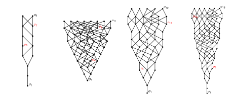
Figure 1. Part of Hasse diagram of $\mathcal{D}(m)$

$F_{4}(1)$                   $F_{4}(2)$                   $E_{6}(2)$                  $E_{7}(1)$

In all cases, we can specify an incomparable pair $(u,w)$ in Table 3, which results in the coincidence of $L:=\ell(u)+\ell(v)$ with $\mbox{e.d.}(G/P_{m})+1$ (where $v=w_{0}ww_{P_{m}}$) after checking $\widetilde{u}\leq\widetilde{w}$ for any $\ell(\widetilde{u})=i$ and $\ell(\widetilde{w})=i+L-1-\dim\mathcal{D}(m)$, for all $1\leq i\leq{L-1\over 2}$ (see [13] for the codes by Mathematica 10.0). It follows that $\mbox{e.d.}(G/P_{m})=\ell(u)+\ell(v)-1$. Comparing the quantity e.d. in Table 1 with the quantity $L$ in Table 3, we conclude the following immediately.

Proposition 4.1.

The good effective divisibility $\mbox{e.d.}(\mathcal{D}(m))$ for $\mathcal{D}$ of exceptional type is precisely given in Table 1.

As we can see from Table 3, all the pairs $(u,w)$ satisfy the property that $u^{-1}$ is again a Grassmannian permutation with respect to another $\mathcal{D}(m^{\prime})$, namely $u^{-1}\in W^{P_{m^{\prime}}}$. Thus if $u$ were less than $w$, then any substring of $w$ that gives $u$ must start with the same digit as for $u$. This observation, together with the Lifting property [2, Proposition 2.2.7]of the Bruhat order, enables us to verify the incomparable pairs even without using computers.

Example 4.2.

For $\mbox{E}_{7}(3)$, we have $u^{-1}\in W^{P_{7}}$, $w=w^{\prime}w^{\prime\prime}$ with $w^{\prime}=s_{624534132456}$ belonging to $W_{P_{7}}$. Hence,

$$u\leq w\Longleftrightarrow u\leq w^{\prime\prime}\Longleftrightarrow s_{7}u\leq s_{7}w^{\prime\prime}.$$

Here the first equivalence follows from the two properties: (1) any reduced expression of $u$ has to start with $s_{7}$, by noting $u^{-1}\in W^{P_{7}}$ and using the third Corollary in [15, section 10.2]; (2) $w^{\prime}$ does not contain $s_{7}$. The second equivalence follows from the Lifting property of the Bruhat order. Now $\bar{u}:=s_{7}u=s_{65432413}$ satisfies similar property to $u$, i.e. $\bar{u}^{-1}\in W^{P_{6}}$. Continuously using the equivalence of the above form, we conclude

$$u\leq w\Longleftrightarrow s_{432413}=s_{5}s_{6}s_{7}u\leq s_{532413}\Longleftrightarrow s_{432413}\leq s_{413}=s_{4}s_{1}s_{3},$$

while the last inequality obviously fails to hold. (The last equality is our notation convention.)

Table 3. An incomparable pair $(u,w)$ for $\mathcal{D}(m)$

$\mathcal{D}$	$m$	$u$	$v$	$w=w_{0}vw_{P_{m}}$	$L$
	1	$s_{12321}$	$s_{12342321}$	$s_{2342321}$	13
	2	$s_{1232}$	$s_{12342312312}$	$s_{323432312}$	15
$\mbox{F}_{4}$	3	$s_{4323}$	$s_{43213243243}$	$s_{232123243}$	15
	4	$s_{43234}$	$s_{43213234}$	$s_{3213234}$	13
	1	$s_{65431}$	$s_{13452431}$	$s_{13452431}$	13
	2	$s_{1342}$	$s_{65432451342}$	$s_{3456245342}$	15
$\mbox{E}_{6}$	3	$s_{1345243}$	$s_{65432413}$	$s_{43245643245432413}$	15
	4	$s_{654324}$	$s_{1345624534}$	$s_{5341324564132451324}$	16
	1	$s_{765431}$	$s_{76543245613452431}$	$s_{6543245613452431}$	23
	2	$s_{765432451342}$	$s_{765432451342}$	$s_{564534132456734132456432451342}$	24
	3	$s_{765432413}$	$s_{7654324561345243}$	$s_{6245341324567541324561324532413}$	25
$\mbox{E}_{7}$	4	$s_{76543245134}$	$s_{765432456134524}$	$s_{45624534132456745341324563413245341324}$	26
	5	$s_{76543245}$	$s_{765432456713456245}$	$s_{45624534132456745341324563413245}$	26
	6	$s_{765432456}$	$s_{765432456713456}$	$s_{345624534132456724534132456}$	24
	7	$s_{7654324567}$	$s_{7654324567}$	$s_{13456245341324567}$	20

$\mathcal{D}$	$m$	$u$	$v$	$L$
	1	$s_{876543245613452431}$	$s_{87654324567813456724563452431}$	47
	2	$s_{8765432456713456245342}$	$s_{87654324567813456724563451342}$	51
	3	$s_{87654324567134562453413}$	$s_{8765432456781345672456345243}$	51
	4	$s_{8765432456713456245341324}$	$s_{876543245678134567245634524}$	52
$\mbox{E}_{8}$	5	$s_{8765432456781345672456345}$	$s_{87654324567134562453413245}$	51
	6	$s_{8765432456781345672456}$	$s_{876543245671345624534132456}$	49
	7	$s_{876543245678134567}$	$s_{8765432456713456245341324567}$	46
	8	$s_{876543245678}$	$s_{87654324567134562453413245678}$	41
		$w=w_{0}vw_{P_{m}}$
	$1$	$s_{2456734562453413245678245341324567543245613452431}$
	2	$s_{543245671345624534132456783456245341324567245341324565432451342}$
	3	$s_{2453413245678543245671345624534132456783456245341324567654324561345243}$
	4	$s_{6543245671345624534132456713456245341324565432451342876543245678134567245634524}$
$\mbox{E}_{8}$	5	$s_{765432456713456245341324567564534132456341324543241387654324567134562453413245}$
	6	$s_{7654324567134562453413245678654324567134562453413245671345624534132456}$
	7	$s_{7654324567134562453413245678765432456713456245341324567}$
	8	$s_{7654324567134562453413245678}$

5. Morphisms to rational homogeneous varieties

In this section, we provide applications of good effective divisibility on the non-existence of non-constant morphisms from complex projective manifolds to rational homogeneous varieties. We will prove the main application Theorem 1.4 right after Proposition 5.2, which cares about morphisms to Grassmannians.

Recall $Q_{2n}=SO(2n+2,\mathbb{C})/P_{1}$ is a smooth quadric hypersurface in $\mathbb{P}^{2n+1}$. The proof of the following proposition is from [17, Corollary 5.3].

Proposition 5.1.

Let $M$ be a connected complex projective manifold. If $\mbox{e.d.}(M)\geq 2n$, then any morphism $\varphi:M\to Q_{2n}$ is a constant map.

Proof.

For $G/P_{1}=Q_{2n}$, we let $u=s_{n}\cdots s_{2}s_{1}$ and $w=s_{n+1}s_{n-1}\cdots s_{2}s_{1}$. Then we have $u,w\in W^{P_{1}}$, $X_{u}\cap X^{w}=\varnothing$, $w_{0}uw_{P_{1}}=w$ and $[X_{u}]=[X^{w}]$. Hence,

$$[\varphi^{-1}(X_{u})]\cup[\varphi^{-1}(X^{w})]=\varphi^{*}([X_{u}])\cup\varphi^{*}([X^{w}])=\varphi^{*}([X_{u}]\cup[X^{w}])=0.$$

Since $\mbox{e.d.}(M)\geq 2n=2\ell(u)$, we have $[\varphi^{-1}(X_{u})]=0\in H^{2n}(M)$, so that $\varphi$ is not surjective. Composing with a linear projection from a linear subspace $\Lambda$ of $\mathbb{P}^{2n+1}$ disjoint from $\varphi(M)$ of maximal dimension, we obtain a surjective morphism $\hat{\varphi}:M\to\mathbb{P}^{\dim\varphi(M)}$. Since $\mbox{e.d.}(M)\geq 2n>\mbox{e.d.}(\mathbb{P}^{\dim\varphi(M)})=\dim\varphi(M)$, it follows that $\dim\varphi(M)=0$. Hence, $\varphi$ is a constant. ∎

The next proposition strengthens [16, Proposition 4.7], generalizing [26, Corollary 3.2] and [18, Proposition 2.4], while the proofs are essentially the same as theirs. Recall our notation convention $G/P_{m}=\mathcal{D}(m)$ for $G$ of type $\mathcal{D}$.

Proposition 5.2.

Let $M$ be a connected complex projective manifold, and $\mathcal{D}(m)$ be a Grassmannian of classical type. If $\mbox{e.d.}(M)>\mbox{e.d.}(\mathcal{D}(m))$, then any morphism $\varphi:M\to\mathcal{D}(m)$ is constant.

Proof.

If $\mathcal{D}(m)=D_{n+1}(1)$, then we are done by Proposition 5.1.

If $\mathcal{D}$ is of type $D_{n+1}$ and $m\in\{n,n+1\}$, then we consider $B_{n}(n)$ instead, due to the isomorphisms $D_{n+1}(n)\cong D_{n+1}(n+1)\cong B_{n}(n)$.

For the remaining cases, we always consider the tautological vector bundles $\mathcal{S}^{\vee}$ and $\mathcal{Q}$ over $\mathcal{D}(m)$. They have effective nonzero Chern classes (see e.g. [25, 5]):

$$c(\mathcal{S}^{\vee}) =\sum_{i=0}^{m}c_{i}(\mathcal{S}^{\vee})=\sum_{i=1}^{m}[X_{s_{m-i+1}\cdots s_{m-1}s_{m}}],$$

$$c(\mathcal{Q}) =\sum_{i=0}^{N-m}c_{i}(\mathcal{Q})=\sum_{i=1}^{N-m}a_{i}[X_{v(i)}].$$

Here $v(i)$ denotes the element in $W^{P_{m}}$ that corresponds to the ($k$-strict) partition $(i,0,\cdots,0)$; $N=\mbox{e.d.}(\mathcal{D}(m))+1$ by (3.2) and Theorem 1.1, and $a_{i}\in\{1,2\}$ is up to the type of $G$ and whether $i>n-m$. Then we can write $c(\varphi^{*}(\mathcal{S}^{\vee}))=1+\eta_{1}+\cdots+\eta_{m}$ and $c(\varphi^{*}(\mathcal{Q}))=1+\xi_{1}+\cdots+\xi_{N-m}$ with $\eta_{i},\xi_{i}\in H^{2i}(M)$ being effective classes. Since $1=c(\mathcal{S})\cup c(\mathcal{Q})$, we have $c_{m}(\mathcal{S}^{\vee})\cup c_{N-m}(\mathcal{Q})=0$, implying $\eta_{m}\cup\xi_{N-m}=0$. Since $N=\mbox{e.d.}(\mathcal{D}(m))+1\leq\mbox{e.d.}(M)$, by definition we have $\eta_{m}=0$ or $\xi_{N-m}=0$. By induction we conclude that either $\eta_{1}=0$ or $\xi_{1}=0$ must hold. Notice $\eta_{1}=c_{1}(\varphi^{*}\det\mathcal{S}^{\vee})$ and $\xi_{1}=c_{1}(\varphi^{*}\det\mathcal{Q})$. We consider $\mathcal{L}=\det\mathcal{S}^{\vee}$ if $\eta_{1}=0$, or $\mathcal{L}=\det\mathcal{Q}$ otherwise. In either cases, $\mathcal{L}$ is an ample line bundle over $\mathcal{D}(m)$ with $c_{1}(\varphi^{*}\mathcal{L})=0$. Assume that $\varphi$ is not a constant morphism. Then $\varphi(x)\neq\varphi(y)$ for some points $x,y\in M$. Take an irreducible curve $C$ in $M$ passing through $x$ and $y$. Then $\varphi(C)$ is of dimension one, and $\varphi_{*}([C])$ is a nonzero effective curve class in $H_{2}(\mathcal{D}(m),\mathbb{Z})$. By projection formula, we have

$$0=\varphi_{*}(c_{1}(\varphi^{*}\mathcal{L})\cap[C])=c_{1}(\mathcal{L})\cap\varphi_{*}[C]>0.$$

This implies a contradiction. Hence, $\varphi$ is a constant morphism. ∎

Proof of Theorem 1.4.

By Theorem 1.2, we have $\mbox{e.d.}(G/P)=\mbox{e.d.}(G/P_{m})$ for some $\alpha_{m}\in\Delta\setminus\Delta_{P}$. Recall that $\pi_{m}:G/P\to G/P_{m}=\mathcal{D}(m)$ denotes the natural projection. Then $\pi_{m}\circ\varphi:M\to\mathcal{D}(m)$ is a morphism with $\mbox{e.d.}(M)>\mbox{e.d.}(\mathcal{D}(m))$. Therefore $\pi_{m}\circ\varphi$ is a constant morphism by Proposition 5.2. That is, $\varphi(M)$ is inside a fiber of $\pi_{m}$.

The Dynkin diagram of $\Delta_{P_{m}}=\Delta\setminus\{\alpha_{m}\}$ consists of $r$ connected components of type $\mathcal{D}^{(1)},\cdots,\mathcal{D}^{(r)}$ respectively. Observe that the fiber $P_{m}/P$ is isomorphic to a product $X_{1}\times\cdots\times X_{r}$ with $X_{i}=G^{(i)}/P^{(i)}$ being a rational homogeneous variety (possibly a point) of type $\mathcal{D}^{(i)}$. As long as $X_{r}$ is not a point, we consider the composition $\hat{\pi}$ of the natural projections $X_{1}\times\cdots\times X_{r}\to X_{r}\to G^{(r)}/\hat{P}=:{\mathcal{D}^{(r)}}(\hat{m})$, where the $\hat{P}$ is a maximal parabolic subgroup of $G^{(r)}$ containing $P^{(r)}$. Clearly, either of the following cases must hold: (1) $\mathcal{D}^{(r)}$ has the same Lie type as $\mathcal{D}$, and is of rank $|\mathcal{D}^{(r)}|<|\Delta|$; (2) $\mathcal{D}^{(r)}$ is of type $A$, $\mbox{h}(\mathcal{D}^{(r)})<\mbox{h}(\mathcal{D})-1$. Consequently, we always have $\mbox{e.d.}(G/P)>\mbox{e.d.}(\mathcal{D}^{(r)}(\hat{m}))$. Hence, $\hat{\pi}\circ\varphi(M)$ is again a constant morphism by Proposition 5.2. That is, $\varphi(M)$ is inside the fiber $\hat{\pi}$.

By considering iterated fibrations of $G/P$ and using induction, we conclude that $\varphi$ is a constant morphism. ∎

Remark 5.3.

The notion $\mbox{e.d.}(M)$ can be naturally extended in the setting of Chow rings $A^{*}(M)$ as in [17]. The above propositions can also be directly generalized to morphisms from (possibly singular) projective varieties $M$. The proof of Proposition 5.2 will also work, by adding one sentence “ By Kleiman’s transversality theorem, there exist $g,g^{\prime}\in G$, such that $\varphi^{-1}(gX_{s_{m-i+1}\cdots s_{m-1}s_{m}})$’s and $\varphi^{-1}(g^{\prime}X_{v(i)})$’s are all generically reduced and of the same codimension as the corresponding Schubert varieties; this ensures that $\varphi^{*}([X_{s_{m-i+1}\cdots s_{m-1}s_{m}}])=[\varphi^{-1}(gX_{s_{m-i+1}\cdots s_{m-1}s_{m}})]$ and $\varphi^{*}([X_{v(i)}])=[\varphi^{-1}(gX_{v(i)})]$ are all effective classes in $A^{i}(M)$”.

As a consequence of Theorem 1.4, we obtain Corollary 1.5 and the follow proposition, by directly comparing $\mbox{e.d.}(G/P_{m})$’s using Theorem 1.1.

Corollary 5.4.

Let $G,\widetilde{G}$ be of the same classical type with $\mbox{rank}(G)<\mbox{rank}(\widetilde{G})$. For any parabolic subgroups $P\subset G$ and $\widetilde{P}\subset\widetilde{G}$, there does not exist any non-constant morphism $\widetilde{G}/\widetilde{P}\to G/P$.

References

- [1] N. Bergeron, F. Sottile, A Pieri-type formula for isotropic flag manifolds, Trans. Amer. Math. Soc. 354 (2002), 4815–4829.
- [2] A. Björner, F. Brenti, Combinatorics of Coxeter groups, Graduate Texts in Mathematics, 231. Springer, New York, 2005.
- [3] A.S. Buch, P.-E. Chaput, L.C. Mihalcea and N. Perrin, Positivity of minuscule quantum -theory, preprint available at arXiv: math.AG/2205.08630.
- [4] A.S. Buch, S. Chung, C. Li and L.C. Mihalcea, Euler characteristics in the quantum -theory of flag varieties, Selecta Math. (N.S.) 26 (2020), no. 2, Paper No. 29, 11 pp.
- [5] A.S. Buch, A. Kresch and H. Tamvakis, Quantum Pieri rules for isotropic Grassmannians, Invent. Math. 178, no. 2 (2009): 345–405.
- [6] A.S. Buch and L.C. Mihalcea, Curve neighborhoods of Schubert varieties, J. Differential Geom. 99 (2015), no. 2, 255–283.
- [7] M. Brion, Lectures on the geometry of flag varieties, Topics in cohomological studies of algebraic varieties, 33–85, Trends Math., Birkhäuser, Basel, 2005.
- [8] P.-E. Chaput, L. Manivel and N. Perrin, Quantum cohomology of minuscule homogeneous spaces, Transform. Groups 13 (2008), no. 1, 47–89.
- [9] R.E. Elliott, M.E. Lewers and L.C. Mihalcea, Quantum Schubert polynomials for the flag manifold, Involve 9 (2016), no. 3, 437–451.
- [10] W. Fulton, Young tableaux. With applications to representation theory and geometry, London Mathematical Society Student Texts, 35. Cambridge University Press, Cambridge, 1997.
- [11] W. Fulton, R. Pandharipande, Notes on stable maps and quantum cohomology, Proc. Sympos. Pure Math. 62, Part 2, Amer. Math. Soc., Providence, RI, 1997.
- [12] W. Fulton, C. Woodward, On the quantum product of Schubert classes, J. Algebraic Geom. 13 (2004), no. 4, 641–661.
- [13] H. Hu, C. Li and Z. Liu, Codes for Grassmannians of exceptional type by Mathematica 10.0, https://math.sysu.edu.cn/gagp/czli.
- [14] J.E. Humphreys, Linear algebraic groups, Graduate Texts in Mathematics 21, Springer-Verlag, New York-Berlin, 1975.
- [15] J.E. Humphreys, Introduction to Lie algebras and representation theory, Graduate Texts in Mathematics 9, Springer-Verlag, New York-Berlin, 1980.
- [16] R. Muñoz, G. Occhetta and L.E. Solá Conde, Splitting conjectures for uniform flag bundles, Eur. J. Math. 6 (2020), no. 2, 430–452.
- [17] R. Muñoz, G. Occhetta and L.E. Solá Conde, Maximal disjoint Schubert cycles in rational homogeneous varieties, preprint at arXiv: math.AG/2211.08216.
- [18] A. Naldi, G. Occhetta, Morphisms between Grassmannians, preprint at arXiv: math.AG/2202.11411.
- [19] X. Pan, Triviality and split of vector bundles on rationally connected varieties, Math. Res. Lett. 22 (2015), no. 2, 529–547.
- [20] P. Pragacz, J. Ratajski, A Pieri-type theorem for Lagrangian and odd orthogonal Grassmannians, J. Reine Angew. Math. 476 (1996), 143–189.
- [21] P. Pragacz, J. Ratajski, A Pieri-type formula for even orthogonal Grassmannians, Fund. Math. 178 (2003), no. 1, 49–96.
- [22] V. Ravikumar, Triple intersection formulas for isotropic Grassmannians, Algebra Number Theory 9 (2015), no. 3, 681–723.
- [23] R.M. Shifler, C. Withrow, Minimum quantum degrees for isotropic Grassmannians in types and , Ann. Comb. 26 (2022), no. 2, 453–480.
- [24] F. Stumbo, Minimal length coset representatives for quotients of parabolic subgroups in Coxeter groups, Boll. Unione Mat. Ital. Sez. B Artic. Ric. Mat. (8) 3 (2000), no. 3, 699–715.
- [25] H. Tamvakis, Quantum cohomology of isotropic Grassmannians, Geometric methods in algebra and number theory, 311–338, Progr. Math., 235, Birkhäuser Boston, Boston, MA, 2005.
- [26] H. Tango, On -dimensional projective spaces contained in the Grassmann variety , J. Math. Kyoto Univ. 14 (1974), 415–460.
- [27] H. Thomas, A. Yong, A combinatorial rule for (co)minuscule Schubert calculus, Adv. Math. 222(2009), no. 2, 596–620