SSDNeRF: Semantic Soft Decomposition of Neural Radiance Fields

Abstract

Neural Radiance Fields (NeRFs) encode the radiance in a scene parameterized by the scene’s plenoptic function. This is achieved by using an MLP together with a mapping to a higher-dimensional space, and has been proven to capture scenes with a great level of detail. Naturally, the same parameterization can be used to encode additional properties of the scene, beyond just its radiance. A particularly interesting property in this regard is the semantic decomposition of the scene. We introduce a novel technique for semantic soft decomposition of neural radiance fields (named SSDNeRF) which jointly encodes semantic signals in combination with radiance signals of a scene. Our approach provides a soft decomposition of the scene into semantic parts, enabling us to correctly encode multiple semantic classes blending along the same direction—an impossible feat for existing methods. Not only does this lead to a detailed, 3D semantic representation of the scene, but we also show that the regularizing effects of the MLP used for encoding help to improve the semantic representation. We show state-of-the-art segmentation and reconstruction results on a dataset of common objects and demonstrate how the proposed approach can be applied for high quality temporally consistent video editing and re-compositing on a dataset of casually captured selfie videos.

1 Introduction

Semantic analysis of scenes has been a subject of study since the early days of computer vision [40]. Traditionally, the problem has been posed as 2D image segmentation or matting in 2D image space. These methods have been shown to facilitate numerous image editing applications such as compositing foreground objects onto novel backgrounds. However, with the increasing popularity of 3D neural scene representations and image based rendering, lifting semantics to the 3D world becomes increasingly important and opens a wide range of novel image/video editing applications yet to be invented.

Early approaches dedicated to 3D semantic segmentation mainly focused on “traditional” 3D geometry representations like meshes, point clouds or voxel grids. For image editing applications, such approaches would be insufficient, since the color of object boundaries in 2D images are often a combination of foreground and background colors. In the 2D image domain, this is addressed using alpha matting where an alpha value per pixel defines how the foreground and background colors are mixed within a given pixel. This idea can be extended into 3D soft semantic segmentation, where multiple classes can be present for a single pixel: we need to take into account that a camera ray passes through several semantic classes in 3D space. Some classes are visible in the final image, but some are blocked by geometry closer to the camera and others are partially visible. All these interactions need to be taken into account correctly, leading to a final rendered result with smooth segmentation.

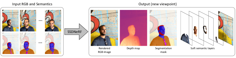
Figure 1: Given a set of RGB images and their segmentation masks computed by a neural network such as Mask-RCNN, SSDNeRF automatically renders an image and its depth map from a novel viewpoint, along with its soft segmentation and soft semantic decomposition. SSDNeRF decomposes a volumetric representation of the scene, thereby lifting semantic segmentation from 2D to 3D.

This is similar in spirit to material density and radiance blending in neural radiance fields, which has been shown to be well handled by a multi-layer perceptron (MLP). We extend the formulation of classical neural radiance fields to incorporate such a soft blending and model densities and colors for each class separately — allowing for an accurate model of complex scenes with several semantic layers.

In this paper, we introduce a semantic soft decomposition of neural radiance fields, SSDNeRF. As illustrated in Figure 1, given a set of images and the results of a 2D semantic segmentation network, we learn a semantic soft decomposition of the 3D scene. This semantic 3D lifting allows the rendering of each semantic layer from a novel view. With our proposed method, we are able to not only trivially decompose scenes semantically, addressing classical computer vision problems such as foreground segmentation, but also edit and re-composite scenes using their 3D content. Since the reasoning happens in 3D space, we can render our edited content consistently into 2D images resolving ambiguities that frame-by-frame 2D methods would be susceptible to. To demonstrate these capabilities, we show various results and applications from casually captured videos and provide comparison with existing state-of-the-art methods. Our typical capture scenario is a video selfie (see Figure 1), and to handle involuntary motions of the captured person, we base our SSDNeRF implementation on deformable neural radiance fields frameworks [26].

Our contributions are: \small{1}⃝ a novel approach to decompose neural radiance fields into a set of soft semantic layers; \small{2}⃝ a set of losses improving the geometric quality of the reconstructed layers; \small{3}⃝ a system to manipulate free viewpoint videos in a temporal consistent manner while respecting fine details and preserving view-dependent effects.

2 Related Work

Semantic scene analysis as well as view synthesis are both well-established fields. Our approach builds upon ideas from semantic segmentation and (compositional) neural radiance fields that we review in the following sections.

2.1 Neural Radiance Fields

Whereas the original neural radiance field [22] implementation focuses on static scenes, we aim to reconstruct scenes captured in a casual setting with a single smartphone camera and where the subject might not be entirely static. Non-rigid NeRF [43] allows for scenes with limited user motion, but makes few assumptions about the motion field and introduces a ‘rigidity’ score for the material. Nerfies [26] has been specifically designed to capture selfie videos into deformable NeRF and uses a restricted deformation model to support and account for minimal, involuntary user motion. This opens up additional editing capabilities (see [26]), hence we base our deformation model on this work. Many other deformable NeRF approaches have been developed based on requirements we do not aim to request from users such as multi-view data [29] or specific sensors [2]. Another line of work uses explicit face models [7, 10] or body models [25, 27, 28] for better regularization, and thus are applicable only for these specific scenarios. Our approach can be used for full body capture as well as general dynamic scenes and we do not rely on object specific priors. A large number of NeRF extensions have been recently published, see [5] for a review. For example, Mip-NeRF 360 [3] and NeRF++ [49] extend NeRF to render un-bounded scenes, or scenes with a large difference in distance between the closest and farthest scene elements. While it is trivial to integrate these techniques in our formulation, we did not find them essential to produce high quality results in our current setting. Some recent works aim to speed up training and inference time [39, 23, 32], and we base our method on [23], demonstrating fast convergence to reconstruct per-scene radiance fields.

Multiple compositional NeRF approaches have been recently proposed to improve the scalability and efficiency of the rendering process [30, 47, 20, 46]. Closer to our work, a set of compositional approaches [24, 38, 48, 6, 9] enable 3D scene decomposition and manipulation. However, none of these approaches are able to provide accurate soft semantic layers critical for high quality video editing.

2.2 Semantic Segmentation

Natural images can be described as the composition of multiple objects where each pixel belongs to one or more classes. Image matting approaches [18, 19] try to revert this process by decomposing an image into soft layers and disentangling the blending of background and foreground resulting in a pixel color. These approaches are heavily used in image editing software and enable the automation of complex editing tasks such as background replacement.

With the recent advances in deep learning, semantic segmentation techniques have improved significantly allowing to jointly segment a large number of semantic classes [4, 13]. One drawback of these approaches is the generation of hard edges that cannot be easily used for image editing purpose. To overcome this issue, the semantic soft segmentation approach [1] uses a DeepLab feature extractor [4] to condition a spectral matting optimization allowing to decompose an image into soft semantic layers. The other related approach [34] decomposes images into simple layers defined by their color and a vector transparency mask. While these technique produce detailed layers, they are designed for single 2D images and thus are not temporally stable, leading to flickering artifacts when applied to videos. In contrast, our approach uses a Mask-RCNN instance segmentation model [13] as supervision but consolidates the per-image labels using the NeRF framework allowing us to generate soft labels that are spatiotemporally consistent.

Semantic segmentation has also been considered in 3D by semantically segmenting meshes [45], point-clouds [11] or voxels [36]. By jointly optimizing for 3D geometry and semantic segmentation, the interdependence between these tasks can be utilized [12]. Describing data terms as potentials over viewing rays [33] can further enhance the accuracy of the obtained 3D reconstructions. End-to-end learning for semantic 3D reconstruction has also been considered [44, 14]. These methods focus on 3D geometry reconstruction and its semantic segmentation without taking into account novel view synthesis and image based rendering. In contrast, our approach incorporates 3D reconstruction, novel view synthesis and semantic segmentation all within the same network.

Semantic-NeRF [50] is the closest approach to our work. They treat the semantic logits as additional radiance channels (identical to color). In contrast, our proposed approach explicitly models multiple classes of objects in the scene by re-deriving the volume rendering formulation for multiple classes, thereby automatically disentangling the representations of different classes. This enables more effective regularization of the opacity, and allows the rendering and manipulation of individual classes of objects.

3 Method

We propose a novel approach allowing the creation of neural radiance fields composed of soft semantic layers. Instead of generating a single density and radiance field for the scene, our approach produces a density and radiance fields per semantic layer to represent soft transitions between semantic classes (Section 3.1). We also introduce a set of regularizations taking advantage of this decomposition to generate high quality semantic layers (Section 3.2).

3.1 Layer Decomposition

RGB	Hair	Skin	T-shirt	Glasses

Figure 2: Comparison of SNeRF [50] (top) and our SSDNeRF (bottom): rendered RGB image (leftmost column) and decomposed semantic layers (other columns). Contrary to our approach which is well regularized using sparsity priors, SNeRF predicts non-zero logits for all classes at all points including free space, leading to noisy layers.

A neural radiance field (NeRF) [22] is a continuous representation $F:(\mathbf{x},\mathbf{d})\rightarrow(\mathbf{c},\sigma)$, which maps a point $\mathbf{x}\in\mathbb{R}^{3}$ on a viewing ray with direction $\mathbf{d}\in\mathbb{R}^{3}$ to an RGB color $\mathbf{c}\in\mathbb{R}^{3}$ and a density $\sigma\in$. The function $F$ is parametrized by an MLP (multi-layer perceptron) and can be queried at arbitrary points allowing to render a volume by accumulating the color values along camera rays by using the density for alpha compositing.

To decompose a NeRF into a set of $M$ semantic layers, our approach extends this formulation and generates a color and a density value per semantic layer, i.e., $F:(\mathbf{x},\mathbf{d})\rightarrow(\mathbf{c}^{1},\sigma^{1},\ldots,\mathbf{c}^{M},\sigma^{M})$. To disambiguate indices, we denote the index for the different layer $i$ in superscript, the index for the ray sample index $j,k$ in subscript notation—there are no powers required in the following formulas. First, let’s recall the compositing equation to accumulate $N$ samples along a ray $\mathbf{r}$ in the original NeRF formulation [22]:

$$C(\mathbf{r}) =\sum_{j=1}^{N}T_{j}\left(1-\exp\left(-\sigma_{j}\delta_{j}\right)\right)\mathbf{c}_{j},$$ (1)

$$\text{where}\quad T_{j}=\exp\left(-\sum_{k=1}^{j-1}\sigma_{k}\delta_{k}\right),$$

$\sigma_{j}$ and $\mathbf{c}_{j}$ are respectively the densities and colors of the $j^{\text{th}}$ sample point along ray $\mathbf{r}$, and $\delta_{k}$ is the distance between the $(k-1)^{\text{th}}$ and $k^{\text{th}}$ ray samples. In our work, this formulation remains unchanged, however, we aim to create a $\sigma$-weighted average across the different layers: hence, at the same point in space the resulting accumulated $\sigma$ value should be the sum of the material density of all the layers and the resulting color should be weighted by the respective layer densities. The density $\sigma$ is exactly the aforementioned sum, and the color $\mathbf{c}$ is accumulated and weighted by each channel’s density and normalized by the sum of overall densities, leading to

$$\sigma=\sum_{i=1}^{M}\sigma^{i}\quad\text{and}\quad\mathbf{c}=\frac{1}{\sigma}\sum_{i=1}^{M}\sigma^{i}\mathbf{c}^{i}.$$ (2)

In addition to rendering all layers, it is possible to render the $i^{\text{th}}$ semantic layer only by using the density $\sigma^{i}$ and color $\mathbf{c}^{i}$ exclusively; the $i^{\text{th}}$ semantic mask can be rendered by using the density $\sigma$ and the color $\frac{\sigma^{i}}{\sigma}$ as

$$S^{i}(\mathbf{r})=\sum_{j=1}^{N}T_{j}\left(1-\exp\left(-\sigma_{j}\delta_{j}\right)\right)\frac{\sigma^{i}_{j}}{\sigma_{j}},$$ (3)

where $\sigma^{i}_{j}$ is the density for semantic layer $i$ at sample point $j$ along ray $\mathbf{r}$. We only provide this abbreviated intuitive argument here for the sake of space and provide the full derivation in the supplementary material. Equation 1, 2, and 3 can be rigorously derived from the volume rendering equation [16] by using multiple material types.

3.2 Losses

NeRF is a notoriously under-constrained representation that needs careful regularization to produce semantically correct results. Our layer decomposition allows each layer to be regularized independently. During training we minimize a set of losses, each playing a critical role in the optimization process. The full loss function is expressed as

$$\mathcal{L}=\mathcal{L}_{\text{color}}+\lambda_{\text{sem}}\mathcal{L}_{\text{sem}}+\lambda_{\text{sparse}}\mathcal{L}_{\text{sparse}}+\lambda_{\text{group}}\mathcal{L}_{\text{group}},$$ (4)

where the $\lambda$ are hyper-parameters weighting the respective losses. The following sections describe the loss terms.

3.2.1 Color Loss.

We use a color loss similar to NeRF [22] to minimize the difference between the rendered and ground truth images. The loss is formulated as

$$\mathcal{L}_{\text{color}}=\sum_{\mathbf{r}\in\mathcal{R}}\|C(\mathbf{r})-\hat{C}(\mathbf{r})\|^{2},$$ (5)

where $\mathcal{R}$ is the set of rays in each batch, and $C(\mathbf{r})$ and $\hat{C}(\mathbf{r})$ are respectively the estimated and ground truth RGB color for the ray $\mathbf{r}$.

3.2.2 Semantic Loss.

In a similar spirit, we introduce a semantic loss term to minimize the difference between the rendered and ground truth semantic masks, given by $|S^{i}(\mathbf{r})-\hat{S}^{i}(\mathbf{r})|^{\gamma}$, where $S^{i}(\mathbf{r})$ and $\hat{S}^{i}(\mathbf{r})$ are the $i^{\text{th}}$ channels of the estimated and ground truth semantic segmentation masks, respectively, along the ray $\mathbf{r}$. In practice, the semantic masks used for supervision are generated from a Mask-RCNN model [13] and are prone to containing outliers, hence we use a robust loss with $\gamma\leq 1$. Additionally, to account for class imbalances, we weigh each class separately using its instantaneous recall (i.e., within each training batch) [42] leading to

$$\mathcal{L}_{\text{sem}} =\sum_{\mathbf{r}\in\mathcal{R}}\sum_{i=1}^{M}(1-R^{i})|S^{i}(\mathbf{r})-\hat{S}^{i}(\mathbf{r})|^{\gamma},\quad\gamma=1,$$ (6)

where $R^{i}=\frac{TP^{i}}{P^{i}}$ is the recall of class $i$, i.e., the ratio of true positives $TP$ to all positives $P$ of that class.

3.2.3 Sparsity Loss.

Without further regularization, the reconstructed models are prone to semi-transparent material close to training camera positions and in mid-air (as will be shown in the ablation study in the experiments section). These are over-fitting artifacts that frequently originate from incorrectly modeled viewpoint-dependent effects. To reduce the occurrence of such partial opacities, we introduce a sparsity loss that favors solutions where opacity is trending towards 0 or 1. This sparsity loss is defined as

$$\mathcal{L}_{\text{sparse}}=\sum_{\mathbf{r}\in\mathcal{R}}\sum_{i=1}^{M}\sum_{j=1}^{N}\bigg{(} |1-\exp(-\sigma^{i}_{j}\delta_{j})|^{\gamma}+$$

$$|\exp(-\sigma^{i}_{j}\delta_{j})|^{\gamma}\bigg{)},\quad\gamma<1.$$ (7)

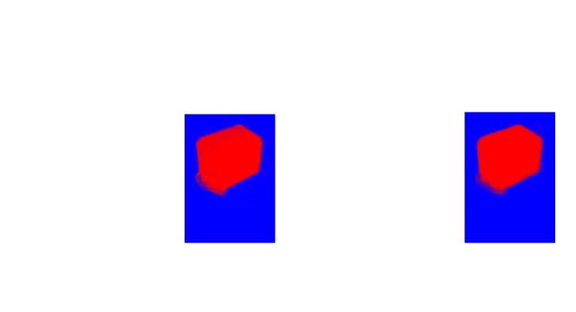
Figure 3: Qualitative comparison between SNeRF and our SSDNeRF on the CO3D dataset showing reconstruction of the foreground layer and the predicted semantic probabilities. Top row shows ground-truth images and input masks. SSDNeRF achieves a much cleaner decomposition into layers.

3.2.4 Group Sparsity Loss.

Whereas the 2D semantic segmentation masks are noisy, we do know that most of the time very few semantic classes should be present at any point in space. We formulate this desired property in an additional regularization term minimizing the co-occurrence of opacity between semantic layers. We use a group sparsity loss for this purpose, favoring solutions where only one opacity value is trending toward $1$ and the others toward $0$ for each sample, defined as

$$\mathcal{L}_{\text{group}}=\sum_{\mathbf{r}\in\mathcal{R}}\sum_{i=1}^{M}\sum_{j=1}^{N}|1-\exp(-\sigma^{i}_{j}\delta_{j})|^{\gamma},\quad\gamma<1.$$ (8)

4 Experiments

This section describes our experiments and presents the results of our method. We begin with the implementation details, establish comparisons with existing methods, and finally, show novel applications enabled by our method.

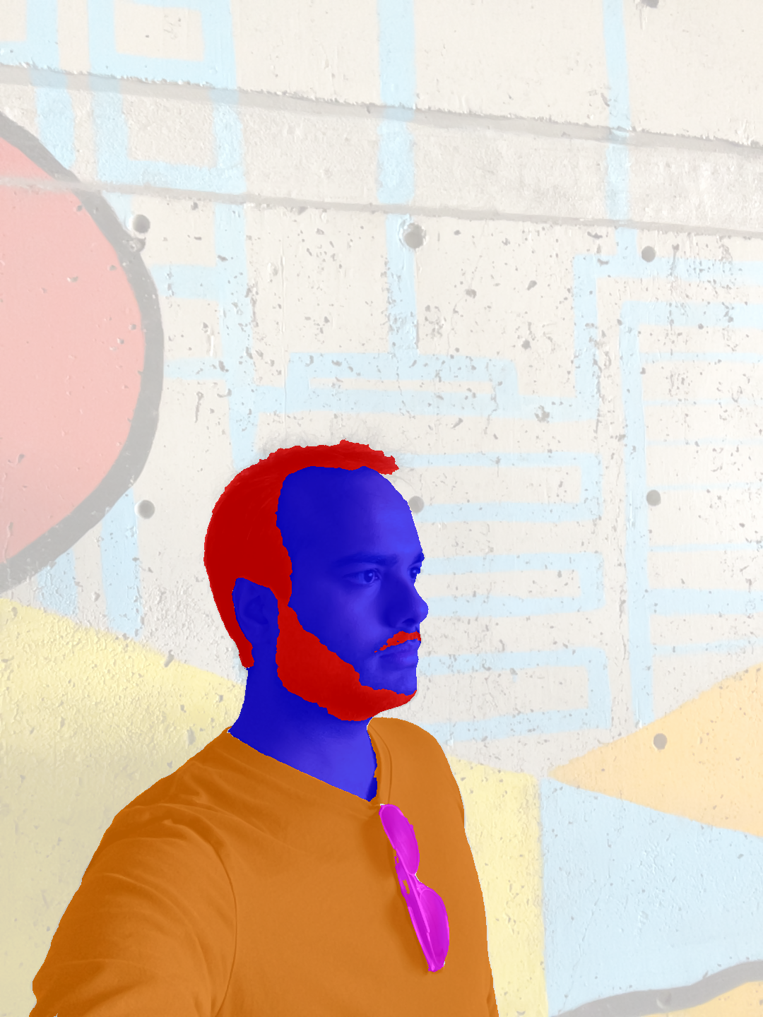
RGB	Semantics	close-up	RGB	Semantics	close-up
SNeRF [50]			SSDNeRF (ours)

Figure 4: Comparison of the proposed SSDNeRF with SNeRF [50], showing reconstructed RGB, semantics, and a close-up view of the semantics. SNeRF treats the semantic logits as additional radiance-like channels, and is trained with a cross-entropy loss with hard (one-hot) labels. In contrast, SSDNeRF formulates different semantic layers as separate opacities and colors, and can correctly handle soft labels, allowing for a decomposition of the scene into layers (Figure 2).

4.1 Implementation Details

We based our implementation on the deformable NeRF framework presented in [26]. Our decomposition framework is fully compatible with the most recent NeRF extensions and can be trivially integrated into [41], a re-implementation of [23]. The network architecture is given in the supplementary material. Given the input images, our approach runs in a fully automatic manner.

4.2 Datasets

We show results on two datasets. The first is a set of face-capture videos using the front camera of an iPhone 12 at a range of resolutions from $1440\times 1080$ to $3840\times 2160$. We filter blurry frames using the variance of the image Laplacian and use COLMAP [35] to estimate the intrinsic and extrinsic camera parameters. To generate the supervision for the semantic layers, we use a Mask-RCNN instance segmentation model [13] trained on a total of 39 classes. For our experiments, we use a subset of 5 classes: skin, hair, T-shirt, hoodie, and glasses. Pixels not containing any instance of the selected classes are labeled background, giving us a total of 6 classes. Not all classes are present in every capture. Due to the casual setting of the face captures, the subjects do move a little during the capture process, requiring a deformation model.

We also show results on a variety of single-scene sequences from the CO3D [31] dataset. Each scene contains a single object with a background, with 100 training and validation images and semantic labels (2 classes: foreground and background). The CO3D dataset contains static scenes, and we do not use a deformation model.

Scene	SSDNeRF		SNeRF
	PSNR	mIoU	PSNR	mIoU
Apple	30.7	0.99	30.2	0.98
Ball	29.0	0.95	29.9	0.95
Bench	28.5	0.98	28.7	0.95
Book	28.2	0.96	27.5	0.94
Orange	26.0	0.98	25.7	0.97
Hydrant	22.0	0.96	21.8	0.93
Teddybear	29.8	0.99	29.8	0.97
Toaster	18.32	0.91	18.24	0.90

Table 1: CO3D dataset: Image PSNR and segmentation mean IoU

4.2.1 Training

We train the different models on an NVidia RTX 3080 GPU for 50k iterations of the Adam optimizer [17] with a learning rate of $10^{-2}$, $\beta_{1}=0.9$, and $\beta_{2}=0.99$. During training, we use 2048 random rays from an image in each batch. We use $\gamma=1$ for the semantic loss, and $\gamma=0.8$ for sparsity and group sparsity. The weights for the losses are $\lambda_{\text{color}}=1$, $\lambda_{\text{sem}}=10^{-1}$, $\lambda_{\text{sparse}}=10^{-3}$, and $\lambda_{\text{group}}=10^{-3}$.

4.3 Evaluation

To evaluate our SSDNeRF approach, we compare it with several existing state-of-the-art methods for view synthesis and (soft) segmentation. We use the exact same input, training and testing data for all the methods. We also provide a qualitative ablation study of the different losses used for training our models.

4.3.1 SSDNeRF vs. SNeRF

The proposed SSDNeRF offers two key advantages over SNeRF [50].

First, SSDNeRF formulates semantics using multiple densities, while SNeRF models semantic logits as additional radiance-like channels, composited in the same way as the color. This enables SSDNeRF to achieve a clean decomposition of the radiance field into layers. SNeRF is not built for this use-case – we formulate a way to extract layers from it by modifying the compositing equation to remove some of the radiance contribution of 3D points based on the predicted semantic logits at those points. Figures 2 and 3 compare the decomposition of images into semantic layers of our method with SNeRF on face captures and the CO3D dataset, resp. Because the semantic logits are unbounded, SNeRF allows low density regions to disproportionately impact the semantics. This results in good images and masks as long as all the layers are rendered together, since high-value logits dominate. However, when the contributions of some classes are removed, artifacts start becoming visible – we refer to the supplementary material for further details.

Second, SSDNeRF uses a robust loss function for supervision of the semantics, enabling it to produce soft labels, which are necessary to handle classes like hair. SNeRF, on the other hand, uses a cross-entropy loss, resulting in hard labels. Figures 4 and 3 compare the semantics from our method against SNeRF [50] on the face captures and on the CO3D, resp. Table 1 evaluates the PSNR of the reconstruction and mean IoU of the predicted segmentation masks on several scans from the CO3D [31] dataset showing competitive performance.

The hashed-grid formulation of [23] used in SSDNeRF trains faster and achieves better results than NeRF [22], upon which the original SNeRF implementation is based. We therefore re-implement SNeRF with this formulation for fair comparison.

(a) Input

(b) [19]

(c) [1]

(d) Ours

Figure 5: Comparison with existing methods: (a) input, (b) results by Spectral Matting [19], (c) by Semantic Soft Segmentation [1], (d) our results. The soft segments are visualized by assigning a solid color to each segment and mixing them using alphas. Since  [1, 19] are 2D color-based, semantic classes aren’t always well-preserved, resulting in inaccurate layers in contrast to our 3D approach.

4.3.2 SSDNeRF vs. Spectral Matting Techniques

We also compare our approach to existing soft segmentation methods. Figure 5 shows a comparison with Spectral Matting [19] and Semantic Soft Segmentation [1]. While these approaches are able to generate soft segmentation masks that respect image details, they are prone to mix different semantic classes together as they are 2D-based and use color consistency to propagate labels. Moreover, these approaches are not temporally stable and cannot be directly applied for video editing tasks (see supplementary video).

4.3.3 SSDNeRF vs Mask-RCNN [13].

In Figure 6, we compare our results with the semantic masks generated by Mask-RCNN. By consolidating the Mask-RCNN labels using multiple views, our approach generates outlier-free results as well as soft boundaries.

4.3.4 Qualitative ablation study

We show the effect of the proposed regularizers in Figure 7. The baseline (with only the color and semantic losses) produces an appropriate RGB and semantic reconstruction, but the individual semantic layers contain “floater” artifacts. These floaters are occluded by other visible parts of the scene when rendering the entire scene, but become visible when rendering individual layers. The proposed regularizers significantly reduce these artifacts, and the final SSDNeRF result (with both regularizers, last row) produces better results than the baseline and those obtained using each regularizer separately.

Figure 6: Visualization of (a) input views, (b) our reconstructions, (c) semantic segmentations from Mask-RCNN (used as input), (d) predicted semantics by our approach. Our approach aggregates the semantic segmentation results from multiple views. This allows to handle segmentation outliers: see the incorrect segmentations shown by the green arrows in column (c) and how they are robustly recovered in our results in column (d). This allows to produce soft segmentation masks that are temporally stable (see supp. video).

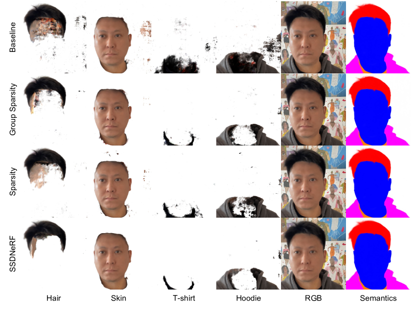
Figure 7: Ablation of the proposed regularizers: adding the regularization terms improves the reconstruction quality of each of the individual layers (see hair, skin, T-shirt, and hoodie columns), without adversely affecting the reconstructed image and semantics (see RGB and semantic columns).

Original colors	Temporally consistent edit

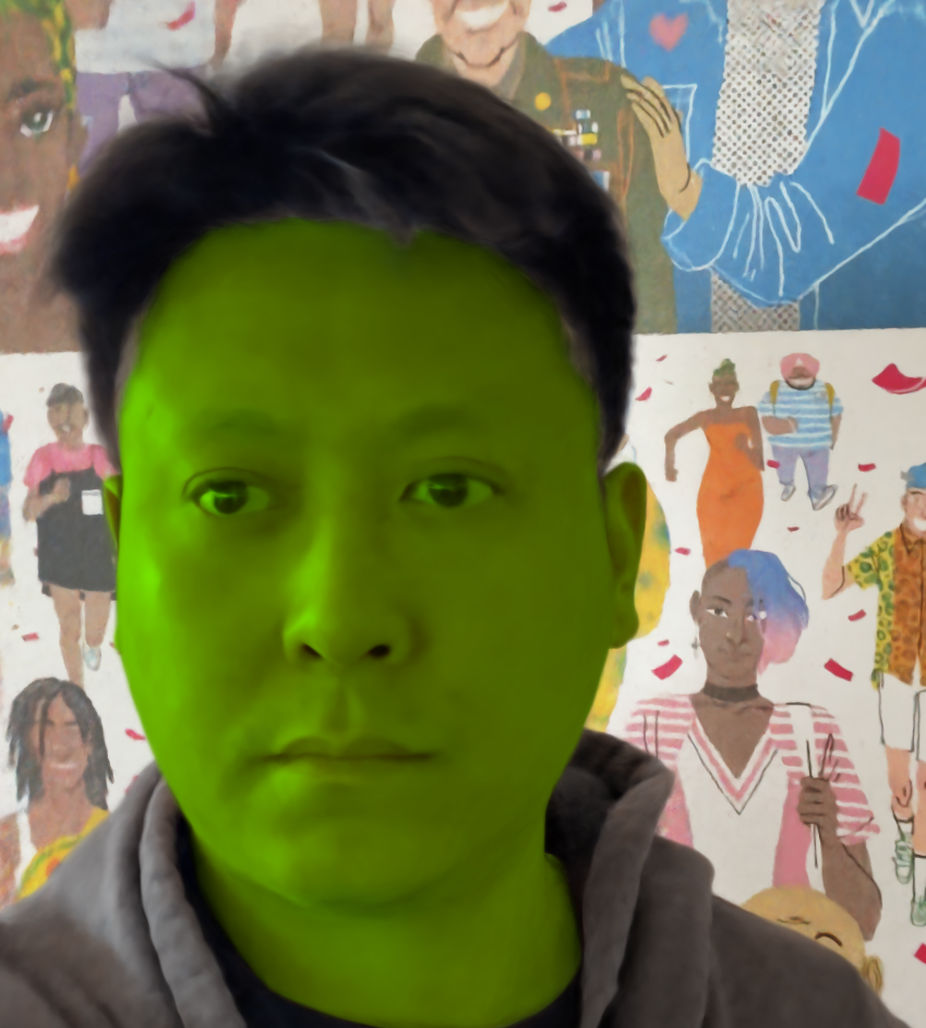
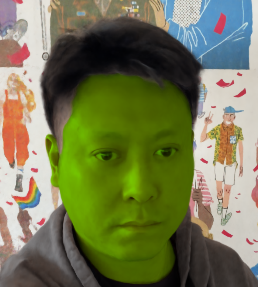
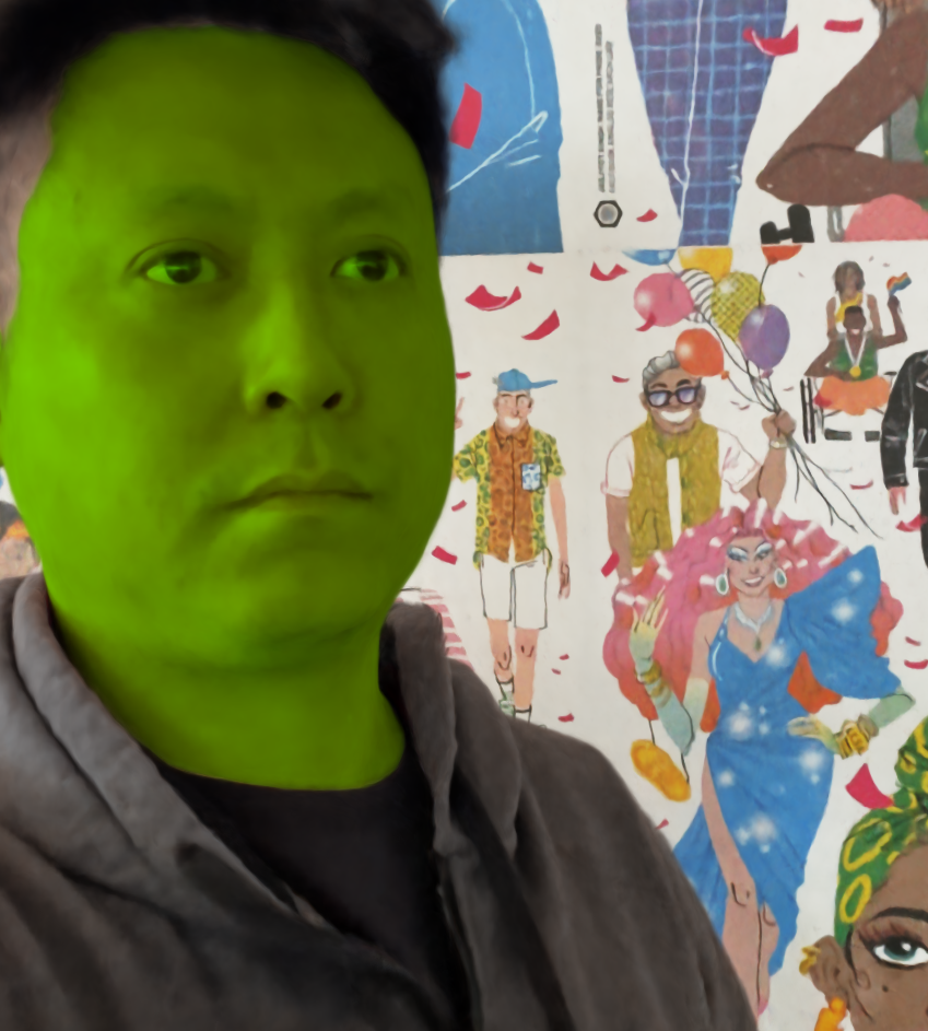
Figure 8: Examples of temporally consistent video editing. Using the semantics allows us to trivially re-color all pixels of a particular class in a temporally and spatially consistent manner without affecting others.

4.4 Video Editing Results

In this section, we show that our approach enables several video editing applications and produces photorealistic results that are temporally and spatially stable. We demonstrate three types of edits: \small{1}⃝ appearance manipulation; \small{2}⃝ geometry manipulation; and \small{3}⃝ camera manipulation.

4.4.1 Appearance Editing.

Our extracted soft semantic layers allow us to trivially re-color all pixels of a particular class without affecting others. Figure 8 shows examples of temporally consistent video edits where we transform the color of different classes.

Figure 9: Geometry editing: the semantic layers produced by our method can be independently modified geometrically without affecting other layers. We translate (top row) and rotate (bottom row) the geometry belonging to the hair, skin, shirt, and glasses layers while keeping the background fixed. The rightmost column shows extreme edits. Translating by a large distance can remove the object from the view frustum entirely (f). Extreme edits have limitations, for example, rotating by too large angles brings the back of the head into the view, but since it was not visible in the training views, the head looks incomplete (g).

4.4.2 Geometry Editing.

One benefit of the compositional nature of our approach is the ability to manipulate objects in 3D. In Figure 9 we demonstrate that objects can be geometrically manipulated (here with a rigid 3D transformation), or even completely removed from the scene. We achieve this by sampling the radiance field a second time at the transformed coordinates, using the original samples of the background class, and the transformed samples for the foreground classes (hair, skin, shirt, and glasses), before compositing along the ray. Visually speaking, this provides novel images where the 3D pose of the person is modified, while the background is kept unchanged. Artifacts show up when the parts of the scene that are not seen in the training views (such as the back of the head in the rightmost column) become visible.

4.4.3 Camera Editing.

Editing extrinsic and intrinsic camera parameters can be easily achieved with NeRF approaches. This allows to generate interesting cinematographic effects such as the dolly zoom effect (see Figure 10). This effect is best demonstrated using video; in the supplementary video, we show that our approach can generate photorealistic novel views and reconstruct the training views with high PSNR.

Figure 10: Dolly zoom effect: the camera simultaneously moves towards the object and reduces its focal length to keep the object size fixed, causing the background to appear to move

5 Limitations and Future Work

Our approach relies on semantic masks generated by Mask-RCNN [13]. While our approach is fairly robust to outliers, as demonstrated in Figure 6, the results might degrade for challenging scenes where Mask-RCNN consistently predicts wrong classes. One avenue of future work would be to reduce the dependency of our approach on Mask-RCNN and train it in an unsupervised manner, similar to [34]. While we have focused our work on encoding semantic segmentation masks, other interesting semantic information could be consolidated in the same way, such as keypoint heatmaps [15], UV maps [8], or NOX maps [37], creating videos with a rich set of temporally and spatially consistent labels.

6 Conclusion

We present a new approach for representing 3D scenes with multiple encoded classes, estimating density and radiance fields for each semantic layer. We leverage a supervised training scheme with initial 2D segmentation masks from a Mask-RCNN model to train such a Semantic Soft Decomposition of Neural Radiance Fields (SSDNeRF). More importantly, we introduce the sparsity and group sparsity losses to avoid a semi-transparent material and reduce the cross-talk between layers, respectively. Experimental results demonstrate the effectiveness and superiority of the proposed SSDNeRF, compared to previous segmentation and NeRF methods. Furthermore, our approach enables 3D scene editing or re-composition, such as changing the background, object re-colorization, and geometric manipulation, in a temporally consistent manner and from novel viewpoints. Finally, we believe that the ability of our approach to generate photorealistic camera, appearance and geometric manipulations will open the door to the capture and generation of a large dataset of dynamic scenes, containing RGB images, depth maps as well as a rich set of semantic labels.

Appendix A Network Architecture

Our implementation is based on [41], a re-implementation of [23]. We extend the NeRF architecture by having $M$ color and density outputs, where $M$ is the number of segmentation layers. Additionally, we extend it with a deformation field similar to by [26], which uses a screw axis representation of rigid transformations. Similar to [26], we use a regularizer on the Laplacian of the deformation field. Figure 11 shows our network architecture, and Figure 12. When $M=1$ (using a single class upon removing the semantic loss and the proposed regularizers), our network architecture reduces to [41].

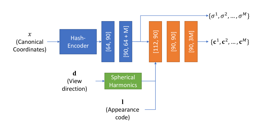
Figure 11: SSDNeRF architecture: at each point $\mathbf{x}$ in the canonical frame with view direction $\mathbf{d}$ and appearance code $\mathbf{l}$, our method predicts colors $\mathbf{c}^{i}$ and opacities $\sigma^{i}$ for each semantic class.

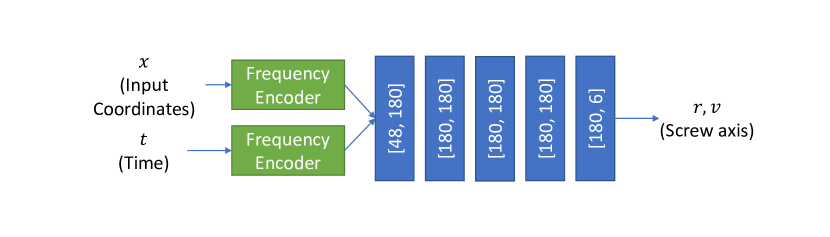
Figure 12: SSDNeRF deformation field: at each point $\mathbf{x}$ at time $t$, our deformation field outputs screw axis parameters $r,v$.

Appendix B Derivation of Compositing Equations

B.1 NeRF [22] Image Reconstruction.

The compositing formula proposed in the original NeRF publication [22] can be derived from the volume rendering integral [21]. We parameterize a ray as $\mathbf{r}(t)=\mathbf{o}+t\mathbf{d}$, where $\mathbf{o}$ is the ray origin and $\mathbf{d}$ the ray direction. The expected color $C(\mathbf{r})$ with near and far bounds $t_{n}$ and $t_{f}$ is

$$C(\mathbf{r}) =\int_{t_{n}}^{t_{f}}T(t)\sigma(t)\mathbf{c}(t)dt,$$

$$\text{where}\quad T(t)=\exp\left(-\int_{t_{n}}^{t}\sigma(s)ds\right).$$ (9)

We discretize the ray in $N$ segments and assume the color and density to be constant along the segment leading to

$$C (\mathbf{r})=\sum_{j=1}^{N}\int_{t_{j}}^{t_{j+1}}T(t)\sigma_{j}\mathbf{c}_{j}dt$$ (10)

$$=\sum_{j=1}^{N}T(t_{j})\left(\int_{t_{j}}^{t_{j+1}}\exp\left(-\int_{t_{j}}^{t}\sigma_{j}ds\right)dt\right)\sigma_{j}\mathbf{c}_{j}$$ (11)

$$=\sum_{j=1}^{N}T(t_{j})\left(\int_{t_{j}}^{t_{j+1}}\exp\left(-\sigma_{j}(t-t_{j})\right)dt\right)\sigma_{j}\mathbf{c}_{j}$$ (12)

$$=\sum_{j=1}^{N}T_{j}\left(1-\exp\left(-\sigma_{j}\delta_{j}\right)\right)\mathbf{c}_{j}$$ (13)

where $\delta_{j}=t_{j+1}-t_{j}$ is the length of the $j^{\text{th}}$ segment and $T_{j}=T(t_{j})=\exp\left(-\sum_{k=1}^{j-1}\sigma_{k}\delta_{k}\right)$.

B.2 SSDNeRF Image Reconstruction.

To decompose a NeRF into a set of $M$ semantic layers, our approach extends this formulation and generates a color and a density value per layer $F:(\mathbf{x},\mathbf{d})\rightarrow(\mathbf{c}^{1},\sigma^{1},\ldots,\mathbf{c}^{M},\sigma^{M})$. The compositing equation for $M$ layers then becomes

$$C(\mathbf{r}) =\int_{t_{n}}^{t_{f}}T(t)\sum_{i=1}^{M}\sigma^{i}(t)\mathbf{c}^{i}(t)dt,$$

$$\text{where}\quad T(t)=\exp\left(-\int_{t_{n}}^{t}\sum_{i=1}^{M}\sigma^{i}(s)ds\right).$$ (14)

Similarly, we discretize the ray into $N$ segments and assume the color and density to be constant along the segment, leading to

$$C(\mathbf{r})=\sum_{j=1}^{N}\int_{t_{j}}^{t_{j+1}}T(t)\sum_{i=1}^{M}\sigma^{i}_{j}\mathbf{c}^{i}_{j}dt$$ (15)

$$= \sum_{j=1}^{N}T(t_{j})\left(\int_{t_{j}}^{t_{j+1}}\exp\left(-\int_{t_{j}}^{t}\sum_{i=1}^{M}\sigma^{i}_{j}ds\right)dt\right)\sum_{i=1}^{M}\sigma^{i}_{j}\mathbf{c}^{i}_{j}$$ (16)

$$= \sum_{j=1}^{N}T(t_{j})\left(\int_{t_{j}}^{t_{j+1}}\exp\left(-\sum_{i=1}^{M}\sigma^{i}_{j}(t-t_{j})\right)dt\right)\sum_{i=1}^{M}\sigma^{i}_{j}\mathbf{c}^{i}_{j}$$ (17)

$$= \sum_{j=1}^{N}T_{j}\left(1-\exp\left(-\sum_{i=1}^{M}\sigma^{i}_{j}\delta_{j}\right)\right)\frac{\sum_{i=1}^{M}\sigma^{i}_{j}\mathbf{c}^{i}_{j}}{\sum_{i=1}^{M}\sigma^{i}_{j}},$$ (18)

where $T_{j}=T(t_{j})=\exp\left(-\sum_{k=1}^{j-1}\sum_{i=1}^{M}\sigma^{i}_{k}\delta_{k}\right)$.

B.3 SSDNeRF Layer Reconstruction.

Generating the $i^{\text{th}}$ layer can be easily achieved by keeping the density of the $i^{\text{th}}$ layer the same and setting the density of other layers to $0$ leading to

$$C^{i}(\mathbf{r}) =\sum_{j=1}^{N}T^{i}_{j}\left(1-\exp\left(-\sigma^{i}_{j}\delta_{j}\right)\right)\mathbf{c}^{i}_{j},$$ (19)

where $T^{i}_{j}=\exp\left(-\sum_{k=1}^{j-1}\sigma^{i}_{k}\delta_{k}\right)$. In a similar spirit, generating the $i^{\text{th}}$ segmentation mask can be achieved by setting the color to $1$ for the $i^{\text{th}}$ layer and the color of the other layers to $0$ leading to

$$S^{i}(\mathbf{r}) =\sum_{j=1}^{N}T_{j}\left(1-\exp\left(-\sum_{i=1}^{M}\sigma^{i}_{j}\delta_{j}\right)\right)\frac{\sigma^{i}_{j}}{\sum_{i=1}^{M}\sigma^{i}_{j}}.$$ (20)

B.4 SNeRF Layer Reconstruction.

The original implementation of SNeRF [50] does not generate disentangled segmentation layers. To compare our approach to SNeRF we modify its compositing equation to remove the radiance contribution of some 3D points based on the predicted semantic class probabilities at those points. More formally, we reweight the density by the class probability leading to

$$C^{i}(\mathbf{r}) =\int_{t_{n}}^{t_{f}}T^{i}(t)p^{i}(t)\sigma(t)\mathbf{c}(t)dt,$$

$$\text{where}\quad T^{i}(t)=\exp\left(-\int_{t_{n}}^{t}p^{i}(s)\sigma(s)ds\right),$$ (21)

where $p^{i}(t)$ is the probability of the $i^{\text{th}}$ class at location $t$. We discretize the ray into $N$ segments and assume the color, density, and probability to be constant along the segment, leading to

$$C^{i}(\mathbf{r})=\sum_{j=1}^{N}\int_{t_{j}}^{t_{j+1}}T^{i}(t)p^{i}_{j}\sigma_{j}\mathbf{c}_{j}dt$$ (22)

$$= \sum_{j=1}^{N}T^{i}(t_{j})\left(\int_{t_{j}}^{t_{j+1}}\exp\left(-\int_{t_{j}}^{t}p^{i}_{j}\sigma_{j}ds\right)dt\right)p^{i}_{j}\sigma_{j}\mathbf{c}_{j}$$ (23)

$$= \sum_{j=1}^{N}T^{i}(t_{j})\left(\int_{t_{j}}^{t_{j+1}}\exp\left(-p^{i}_{j}\sigma_{j}(t-t_{j})\right)dt\right)p^{i}_{j}\sigma_{j}\mathbf{c}_{j}$$ (24)

$$= \sum_{j=1}^{N}T^{i}_{j}\left(1-\exp\left(-p^{i}_{j}\sigma_{j}\delta_{j}\right)\right)\mathbf{c}_{j},$$ (25)

where $T^{i}_{j}=T^{i}(t_{j})=\exp\left(-\sum_{k=1}^{j-1}p^{i}_{k}\sigma_{k}\delta_{k}\right)$.

References

- [1] Yağız Aksoy, Tae-Hyun Oh, Sylvain Paris, Marc Pollefeys, and Wojciech Matusik. Semantic soft segmentation. TOG, 2018.
- [2] Benjamin Attal, Eliot Laidlaw, Aaron Gokaslan, Changil Kim, Christian Richardt, James Tompkin, and Matthew O’Toole. Törf: Time-of-flight radiance fields for dynamic scene view synthesis. NeurIPS, 2021.
- [3] Jonathan T. Barron, Ben Mildenhall, Dor Verbin, Pratul P. Srinivasan, and Peter Hedman. Mip-NeRF 360: Unbounded anti-aliased neural radiance fields. arXiv, 2021.
- [4] Liang-Chieh Chen, George Papandreou, Iasonas Kokkinos, Kevin Murphy, and Alan L. Yuille. DeepLab: Semantic image segmentation with deep convolutional nets, atrous convolution, and fully connected CRFs. TPAMI, 2017.
- [5] Frank Dellaert and Lin Yen-Chen. Neural volume rendering: Nerf and beyond. arXiv, 2020.
- [6] Cathrin Elich, Martin R Oswald, Marc Pollefeys, and Joerg Stueckler. Weakly supervised learning of multi-object 3d scene decompositions using deep shape priors. CoRR, 2020.
- [7] Guy Gafni, Justus Thies, Michael Zollhöfer, and Matthias Nießner. Dynamic neural radiance fields for monocular 4D facial avatar reconstruction. In CVPR, 2021.
- [8] Rıza Alp Güler, Natalia Neverova, and Iasonas Kokkinos. Densepose: Dense human pose estimation in the wild. In CVPR, 2018.
- [9] Michelle Guo, Alireza Fathi, Jiajun Wu, and Thomas Funkhouser. Object-centric neural scene rendering. arXiv, 2020.
- [10] Yudong Guo, Keyu Chen, Sen Liang, Yongjin Liu, Hujun Bao, and Juyong Zhang. AD-NeRF: Audio driven neural radiance fields for talking head synthesis. In ICCV, 2021.
- [11] Timo Hackel, Jan D Wegner, and Konrad Schindler. Fast semantic segmentation of 3D point clouds with strongly varying density. ISPRS annals of the photogrammetry, remote sensing and spatial information sciences, 2016.
- [12] Christian Häne, Christopher Zach, Andrea Cohen, and Marc Pollefeys. Dense semantic 3D reconstruction. TPAMI, 2016.
- [13] Kaiming He, Georgia Gkioxari, Piotr Dollár, and Ross Girshick. Mask R-CNN. In ICCV, 2017.
- [14] Ji Hou, Angela Dai, and Matthias Nießner. 3D-SIS: 3D semantic instance segmentation of RGB-D scans. In CVPR, 2019.
- [15] Hossam Isack, Christian Haene, Cem Keskin, Sofien Bouaziz, Yuri Boykov, Shahram Izadi, and Sameh Khamis. Repose: Learning deep kinematic priors for fast human pose estimation. arXiv, 2020.
- [16] James T. Kajiya and Brian P Von Herzen. Ray tracing volume densities. In SIGGRAPH, 1984.
- [17] Diederik P. Kingma and Jimmy Ba. Adam: A method for stochastic optimization. In Yoshua Bengio and Yann LeCun, editors, ICLR, 2015.
- [18] Anat Levin, Dani Lischinski, and Yair Weiss. A closed-form solution to natural image matting. TPAMI, 2008.
- [19] Anat Levin, Alex Rav-Acha, and Dani Lischinski. Spectral matting. TPAMI, 2008.
- [20] Stephen Lombardi, Tomas Simon, Gabriel Schwartz, Michael Zollhoefer, Yaser Sheikh, and Jason Saragih. Mixture of volumetric primitives for efficient neural rendering. TOG, 2021.
- [21] N. Max. Optical models for direct volume rendering. TVCG, 1995.
- [22] Ben Mildenhall, Pratul P. Srinivasan, Matthew Tancik, Jonathan T. Barron, Ravi Ramamoorthi, and Ren Ng. NeRF: Representing scenes as neural radiance fields for view synthesis. In ECCV, 2020.
- [23] Thomas Müller, Alex Evans, Christoph Schied, and Alexander Keller. Instant neural graphics primitives with a multiresolution hash encoding. ACM Trans. Graph., 41(4):102:1–102:15, July 2022.
- [24] Michael Niemeyer and Andreas Geiger. Giraffe: Representing scenes as compositional generative neural feature fields. In CVPR, 2021.
- [25] Atsuhiro Noguchi, Xiao Sun, Stephen Lin, and Tatsuya Harada. Neural articulated radiance field. In ICCV, 2021.
- [26] Keunhong Park, Utkarsh Sinha, Jonathan T. Barron, Sofien Bouaziz, Dan B Goldman, Steven M. Seitz, and Ricardo Martin-Brualla. Nerfies: Deformable neural radiance fields. ICCV, 2021.
- [27] Sida Peng, Junting Dong, Qianqian Wang, Shangzhan Zhang, Qing Shuai, Xiaowei Zhou, and Hujun Bao. Animatable neural radiance fields for modeling dynamic human bodies. In ICCV, 2021.
- [28] Sida Peng, Yuanqing Zhang, Yinghao Xu, Qianqian Wang, Qing Shuai, Hujun Bao, and Xiaowei Zhou. Neural body: Implicit neural representations with structured latent codes for novel view synthesis of dynamic humans. In CVPR, 2021.
- [29] Albert Pumarola, Enric Corona, Gerard Pons-Moll, and Francesc Moreno-Noguer. D-NeRF: Neural radiance fields for dynamic scenes. arXiv, 2020.
- [30] Daniel Rebain, Wei Jiang, Soroosh Yazdani, Ke Li, Kwang Moo Yi, and Andrea Tagliasacchi. DeRF: Decomposed radiance fields. In CVPR, 2020.
- [31] Jeremy Reizenstein, Roman Shapovalov, Philipp Henzler, Luca Sbordone, Patrick Labatut, and David Novotny. Common objects in 3d: Large-scale learning and evaluation of real-life 3d category reconstruction. In International Conference on Computer Vision, 2021.
- [32] Sara Fridovich-Keil and Alex Yu, Matthew Tancik, Qinhong Chen, Benjamin Recht, and Angjoo Kanazawa. Plenoxels: Radiance fields without neural networks. In CVPR, 2022.
- [33] Nikolay Savinov, Christian Hane, Lubor Ladicky, and Marc Pollefeys. Semantic 3D reconstruction with continuous regularization and ray potentials using a visibility consistency constraint. In CVPR, 2016.
- [34] Othman Sbai, Camille Couprie, and Mathieu Aubry. Unsupervised image decomposition in vector layers. In ICIP, 2020.
- [35] Johannes Lutz Schönberger and Jan-Michael Frahm. Structure-from-motion revisited. In Conference on Computer Vision and Pattern Recognition (CVPR), 2016.
- [36] Sunando Sengupta, Eric Greveson, Ali Shahrokni, and Philip HS Torr. Urban 3D semantic modelling using stereo vision. In ICRA, 2013.
- [37] Srinath Sridhar, Davis Rempe, Julien Valentin, Bouaziz Sofien, and Leonidas J Guibas. Multiview aggregation for learning category-specific shape reconstruction. NeurIPS, 2019.
- [38] Karl Stelzner, Kristian Kersting, and Adam R Kosiorek. Decomposing 3D scenes into objects via unsupervised volume segmentation. arXiv, 2021.
- [39] Cheng Sun, Min Sun, and Hwann-Tzong Chen. Direct voxel grid optimization: Super-fast convergence for radiance fields reconstruction. arXiv, 2021.
- [40] Richard Szeliski. Computer Vision - Algorithms and Applications, Second Edition. Springer, 2022.
- [41] Jiaxiang Tang. Torch-ngp: a pytorch implementation of instant-ngp, 2022. https://github.com/ashawkey/torch-ngp.
- [42] Junjiao Tian, Niluthpol Chowdhury Mithun, Zachary Seymour, Han-Pang Chiu, and Zsolt Kira. Striking the Right Balance: Recall Loss for Semantic Segmentation. In 2022 International Conference on Robotics and Automation (ICRA), pages 5063–5069, 2022.
- [43] Edgar Tretschk, Ayush Tewari, Vladislav Golyanik, Michael Zollhöfer, Christoph Lassner, and Christian Theobalt. Non-rigid neural radiance fields: Reconstruction and novel view synthesis of a dynamic scene from monocular video. In ICCV, 2021.
- [44] Shubham Tulsiani, Tinghui Zhou, Alexei A Efros, and Jitendra Malik. Multi-view supervision for single-view reconstruction via differentiable ray consistency. In CVPR, 2017.
- [45] Julien Valentin, Vibhav Vineet, Ming-Ming Cheng, David Kim, Jamie Shotton, Pushmeet Kohli, Matthias Nießner, Antonio Criminisi, Shahram Izadi, and Philip Torr. SemanticPaint: Interactive 3D labeling and learning at your fingertips. TOG, 2015.
- [46] Ziyan Wang, Timur Bagautdinov, Stephen Lombardi, Tomas Simon, Jason Saragih, Jessica Hodgins, and Michael Zollhofer. Learning compositional radiance fields of dynamic human heads. In CVPR, 2021.
- [47] Yuanbo Xiangli, Linning Xu, Xingang Pan, Nanxuan Zhao, Anyi Rao, Christian Theobalt, Bo Dai, and Dahua Lin. CityNeRF: Building NeRF at city scale. arXiv, 2021.
- [48] Hong-Xing Yu, Leonidas J Guibas, and Jiajun Wu. Unsupervised discovery of object radiance fields. In ICLR, 2022.
- [49] Kai Zhang, Gernot Riegler, Noah Snavely, and Vladlen Koltun. NeRF++: Analyzing and improving neural radiance fields. arXiv, 2020.
- [50] Shuaifeng Zhi, Tristan Laidlow, Stefan Leutenegger, and Andrew Davison. In-place scene labelling and understanding with implicit scene representation. In ICCV, 2021.