Screening with Persuasion

Abstract

We consider a general nonlinear pricing environment with private information. The seller can control both the signal that the buyers receive about their value and the selling mechanism. We characterize the optimal menu and information structure that jointly maximize the seller’s profits. The optimal screening mechanism has finitely many items even with a continuum of values. We identify sufficient conditions under which the optimal mechanism has a single item.  Thus the seller decreases the variety of items below the efficient level as a by-product of reducing the information rents of the buyer.

Jel Classification: D44, D47, D83, D84.

Keywords: Nonlinear Pricing, Screening, Bayesian Persuasion, Finite Menu, Second-Degree Price Discrimination, Recommender System

1 Introduction

1.1 Motivation

In a world with a large variety of products and hence feasible matches between buyers and products, information can fundamentally affect the match between buyers and products. A notable feature of the digital economy is that sellers, or platforms and intermediaries that sellers use to place their products, commonly have information about the value of the match between any specific product and any specific buyer. In particular, by choosing how much information to disclose to the buyer about the value of the match between product and buyer, a seller can affect both the variety and the prices of the products offered.

We analyze the interaction between information and choice in a classic nonlinear pricing environment. The seller can offer a variety of products that are differentiated by their quality and thereby screen the buyers for their willingness-to-pay. The seller can also control how much information to disclose to the buyers about their willingness-to-pay for the qualities, and thus the seller screens while engaging in Bayesian persuasion.

We characterize the information structure and menu of choices that maximize the expected profit of the seller.  The buyers have a continuum of possible values–their willingness-to-pay for quality. In the absence of any information design, the optimal menu typically offers a continuum of qualities to the buyers who then select given their private information (e.g., as in muro78 and mari84).  By contrast, in the current setting, the seller controls the selling mechanism and the information structure. Importantly, the seller remains constrained in that he cannot observe either values or signal realizations of the buyers.  The selling mechanism could be any (possibly stochastic) menu.  Our main analysis considers the case where the distribution of ex post qualities to be sold by the seller is exogenously given (as in the recent work of lomu22). The seller can create bundles of different qualities to sell to the buyers.  We then extend our results to the case where the seller produces goods with different qualities with a convex cost function, as in the classic analysis of muro78 and mari84.

Our main result (Theorem 1) is a characterization of the optimal information and mechanism design. The seller provides information via monotone pooling, i.e., every value is pooled with a positive mass of nearby values and the pool takes the form of an interval.  There is also monotone pooling of qualities, where each pool of buyers is allocated to a specific pool of qualities. Using the convexity of the information rent, we show that the buyers are pooled into finitely many intervals and are offered a menu with finitely many items. This contrasts with the optimal menu in the absence of information design that contains a continuum of items.

The argument is as follows.  Once one fixes the distribution of expected values induced by an information structure and a distribution of expected qualities, the revenue is pinned down by standard Myersonian arguments.  The problem then reduces to maximizing a linear functional subject to two majorization constraints.  As a first step, we establish that information is optimally given by a monotone partition, where elements of the partition are either intervals (with pooling) or singletons (with full disclosure of the value). This first step follows from fixing the pooled distribution of qualities and observing the problem with one majorization constraint is linear in the distribution of expected values so a maximum is attained at an extreme point of the set of feasible distributions (klms21).  The second step uses an orthogonal variational argument.  Suppose that an interval of values were completely revealed and screened by the seller.  We ask what happens to profit if we pool the allocation of a small interval of values. By construction, distortions in the allocation from the profit-maximizing allocation will only cause second-order distortions to the total virtual surplus. But if we additionally pool a small interval of values into a single expected value, then this causes a first-order decrease in the information rents. Hence, screening an open set of values is never optimal because pooling the values, and consequently the allocation, causes a first-order reduction in the information rents and only second-order distortions on profit.

Theorem 1 establishes that the optimal menu with persuasion is discrete and thus “small” relative to the (continuum) menu in the absence of persuasion. But how small will the optimal menu be?

A second set of results establishes sufficient conditions under which the partitions of values and qualities will be very coarse and thus the number of items in the menu will be small. If the support of the distribution of qualities is bounded, then the optimal menu will be finite (Theorem 2). If the distribution of qualities is convex (i.e., the density is weakly increasing), then a single-item menu is optimal (Theorem 3). More generally, the number of items in the menu is no more than the ratio of the upper bound to the lower bound of the support of the exogenous quality distribution (Proposition 2).  By contrast, with complete disclosure of information there would typically be a continuum of items in the optimal menu.

Our main result goes through unchanged in the classic setting of muro78 where the distribution of qualities for sale is endogenous and the seller has a convex cost of producing quality. The intuition is that the above argument shows that pooling will increase revenue, and with a convex production cost, pooling will additionally reduce cost and so pooling will increase profit. The number of items in the optimal menu will now be sensitive to the convexity of the cost function. We report results for the case where the cost function has a constant elasticity. We show that a single-item menu will always be optimal for a sufficiently high level of cost elasticity, that is any given information structure generates less profit than pooling all values (i.e., providing no information) when the cost elasticity is high enough. Conversely, any given information structure will generate less profit than complete disclosure if the cost elasticity is low enough, i.e. approaching unit elasticity which corresponds to linear costs (Proposition 3).

Our setting reflects three notable features of the digital economy. We already mentioned the fact that the sellers are well-informed about buyers’ values and specifically their match value with the products of the seller. Our analysis considers the extreme case where the buyers only knows the prior and the seller has access to all feasible signals. A second notable feature is that the buyers have the ability to find which items are available at what prices, due to search engines and price comparison sites. Thus, personalized prices (or more generally third-degree price discrimination) are not available, but menu pricing (or more generally second-degree price discrimination) can occur. Finally, particular items, that is quality-price pairs, are recommended to different buyers via recommendation and ranking services. In Section 7, we show that the optimal mechanism can be implemented as an indirect mechanism in the form of a recommender system.

1.2 Related Literature

We analyze a model of nonlinear pricing and consider first the case where the distribution of qualities is exogenous as in the recent work of lomu22.  Subsequently, we establish that our main result continues to hold in the setting of muro78 where the distribution of qualities is endogenous and an increasing function of quality. lomu22 consider a seller who offers fixed quantities of products of different qualities. They show that bundling different qualities, or randomizing the quality assignment via lotteries, can increase the revenue in the presence of irregular type distributions. Pooling is optimal in our setting for all regular and irregular distributions.

In our analysis, the seller can control the information of the buyers and the selling mechanism in which the pooling of qualities is feasible. It therefore combines Bayesian persuasion (kage11) or information design more generally with mechanism design tools. We thus offer a solution to an integrated mechanism and information design problem in a classic economic environment. Perhaps surprisingly given the proximity of the tools as highlighted in the recent work by klms21, we are not aware of other work on optimal pricing combining mechanism and information design.  The closest work is that of bepe07, who consider a seller with many unit-demand buyers. We postpone a detailed discussion to Section 3.2 after we obtain a canonical statement of our problem.

We analyze a second-degree price discrimination problem.  As the seller pools buyers with adjacent values, the seller creates segments within a single aggregate market.  In doing so, the seller makes any item intended for one segment less attractive to the other segments in the same market.   By contrast, bebm15 and hasi22 allow many markets and thus full third-degree price discrimination while offering quality-differentiated products. rosz17 consider the buyer-optimal information structure for a single-item demand and a single aggregate market. Thus, the demand structure and the objective differ from the present work, but they share the focus on creating segments within a single aggregate market.

rayo13 considers a model of social status provision that shares some features with our model. The utility function of an agent before any transfer is a product of their type (or an increasing function of their type) and a social status which is equal to their expected type given some information structure. rayo13 then asks what is the optimal information structure to provide to the agent by a revenue-maximizing monopolist. Thus, the allocation in rayo13 is an information structure rather than a quality allocation. Importantly, the information structure only affects the allocation but not the expectation of the agents regarding their own type.

2 Model

A seller supplies goods of varying quality $q\in\mathbb{R}_{+}$ to a continuum of buyers with mass $1$. The seller has a mass 1 of goods with qualities $q\in[\underline{q},\bar{q}]$ distributed according to

$$Q\in\Delta\left([\underline{q},\bar{q}]\right),$$ (1)

where $0\leq\underline{q}<\bar{q}<\infty$. Thus, the seller can offer a fixed and exogenously given distribution $Q$ of qualities. In Section 6 we extend the analysis to a setting with endogenously chosen quantities as in muro78 and mari84. We introduce the additional notation at that point.

Each buyer has unit demand and a willingness-to-pay, or value ${v}\in\mathbb{R}_{+}$ for quality $q$. The utility net of the payment $p\in\mathbb{R}_{+}$ is:

$$u({v},q,p)\triangleq{v}q-p.$$ (2)

The buyers’ values ${v}\in[\underline{v},\bar{v}]$ are distributed according to

$$F\in\Delta\left([\underline{v},\bar{v}]\right),$$ (3)

where $0\leq\underline{v}<\bar{v}<\infty$, with strictly positive density (i.e., $f(v)>0$ for all $v$). Initially, the buyers and the seller only know the common prior distribution of values.

The seller’s choice has two components: $\left(i\right)$ the seller chooses the information that buyers have about their own value, and $\left(ii\right)$ the seller chooses a direct mechanism (or menu) that specifies the (expected) quality and payments for any reported (expected) value. We now describe these elements in turn.

First, the seller chooses a signal (or information structure):

$$S:\mathbb{R}_{+}\rightarrow\Delta\mathbb{R}_{+},$$ (4)

where $s({v})$ denotes a signal realization observed by a buyer when the value is ${v}$. A buyer’s expected value conditional on the signal realization $s$ is denoted by:

$$w\triangleq\mathbb{E}[{v}\mid s].$$ (5)

Since the utility is linear in $v$, $w$ is a sufficient statistic for determining the buyers’ preferences when they observe signal $s$. The information that the buyers receive about their expected value $w\in\mathbb{R}_{+}$ is represented by a distribution of expected values $G$:

$$G\in\Delta\left([\underline{v},\overline{v}]\right),$$

and $\textit{supp}G$ denotes the support of the distribution $G$.

Second, the seller chooses a menu of qualities and payments. The seller has the ability to shape the distribution of qualities sold by pooling goods of different quality. If the buyers are offered a distribution of qualities, or bundle $B$ with

$$B\in\Delta\left([\underline{q},\overline{q}]\right),$$

then the expected quality offered is:

$$q\triangleq\int_{\underline{q}}^{\bar{q}}tdB(t).$$

If $\int dB(t)dt<1$, then the probability of receiving an object is less than 1. This is of course equivalent to receiving a zero quality good with probability $1-\int dB(t)$. The expected utility of a bundle $B$ net of the payment $p\in\mathbb{R}_{+}$ is:

$$u({w},B,p)={w}\int_{\underline{q}}^{\bar{q}}tdB(t)-p.$$ (6)

A menu (or direct mechanism) with bundles $B\left(\left.\cdot\right|w\right)$ at prices $p\left(w\right)$ for every value $w$ is given by:

$$M\triangleq\left\{(B\left(\left.\cdot\right|w\right),p(w))\right\}_{w\in\mathrm{supp}G},$$ (7)

where a specific bundle $B\left(\left.\cdot\right|w\right)$ generates an expected quality $q\left(w\right)$:

$$q\left(w\right)\triangleq\int_{\underline{q}}^{\bar{q}}tdB\left(\left.t\right|w\right).$$

The menu has to satisfy incentive compatibility and participation constraints:

$$wq(w)-p(w) \geq wq(w^{\prime})-p\left(w^{\prime}\right),\ \ \forall w,w^{\prime}\in\mathrm{supp}G;$$ (8)

$$wq(w)-p(w) \geq 0,\ \ \forall w\in\mathrm{supp}G;$$ (9)

as well as feasibility. Namely, the volume of qualities offered must be weakly less than the volume of qualities the seller has available:

$$\int_{\underline{v}}^{\bar{v}}\int_{q}^{q^{\prime}}dB\left(\left.t\right|w\right)dG(w)\leq\int_{q}^{q^{\prime}}dQ(t),\ \ \forall q,q^{\prime}\in[\underline{q},\bar{q}]$$ (10)

Hence, the total amount of goods of quality in any interval $[q,q^{\prime}]$ offered to the buyers must be weakly less than the goods of the same quality in the seller’s endowment.

We refer to a mechanism as a pair $\left(S,M\right)$ of information structure $S$ and menu $M$. The seller’s problem is to maximize expected profit subject to the above incentive compatibility, participation and feasibility constraints (8)-(10):

$$\Pi\triangleq\max_{\begin{subarray}{c}S:\mathbb{R}_{+}\rightarrow\Delta(\mathbb{R}_{+})\\ \left\{B\left(\left.\cdot\right|w\right),p(w)\right\}\end{subarray}}\mathbb{E}[p(w)].$$ (11)

Since there is no cost, the profit is equal to revenue.

A first significant step in the analysis is to show that the above seller’s problem can be stated entirely in terms of a choice of a pair of distributions over expected values and expected qualities, respectively, subject to the appropriate majorization constraints. The menu, namely allocation $B\left(\left.\cdot\right|w\right)$ and transfer $p(w)$, can be represented entirely in terms of these distributions.

3 A Reformulation with Majorization Constraints

We start with a re-statement of the seller’s problem exploiting standard properties of incentive compatible and feasible mechanisms. This will lead us to state the revenue maximization (11) as an optimization problem subject to two majorization constraints that is bilinear in the distributions of expected values and expected qualities. This reformulation uses familiar insights from myer81 regarding optimal mechanism and klms21 on majorization representations of information structures to obtain a maximization problem subject to majorization constraints. Since we are jointly optimizing in the space of values and qualities (allocations), we obtain two majorization constraints, one for each dimension of the design problem. By contrast earlier work in information design largely focused on optimization problems in a single dimension and thus a single majorization constraint. The presence of two majorization constraints will have significant implications for the nature of the optimal solution. We will discuss those differences at the end of this section.

3.1 Two Majorization Constraints 

The seller’s choice has two components: $\left(i\right)$ the seller chooses the information that buyers have about their own value, and $\left(ii\right)$ the seller chooses a mechanism that specifies the (expected) quality and payments for any reported (expected) value.

Following standard techniques, the incentive compatibility requires that the allocation $q(w)$ is increasing and the payments $p\left(w\right)$ are determined by the allocation rule using the Envelope condition:

$$\mathbb{E}[p(w)]=\int_{\underline{v}}^{\bar{v}}\bigg{(}wq(w)-\int_{\underline{v}}^{w}q(s)ds\bigg{)}dG(w),$$ (12)

where $G$ is the distribution of expected valuations and the second term inside the integral is the buyers’ information rent. Note that $G$ may have gaps but it is without loss of generality to assume that $q$ is defined on the whole domain $[\underline{v},\bar{v}]$ and hence we can pin down payments uniquely with the allocation rule. The seller’s objective is to maximize (12) subject to the constraint that $G$ can be induced by some information structure and the quality assignments are feasible (of course, whether $q(w)$ is feasible depends on $G$).

The buyers’ information structure is summarized by the distribution of expected valuations $G$.  By blac51, Theorem 5, there exists an information structure that induces a distribution $G$ of expected values if and only if $G$ is a mean-preserving contraction of $F$, i.e.,

$$\int_{v}^{\overline{v}}F({t})dt\leq\int_{v}^{\overline{v}}G({t})dt\text{, }\forall{v}\in[\underline{v},\bar{v}],$$

with equality for $v=\underline{v}$.  If $G~{}$is a mean-preserving contraction of $F$ (or $G$ majorizes $F$), we write $G\succ F$. Following shsh07 (Chapter 3), we have that $G\succ F$ if and only if $F^{-1}\succ G^{-1}$.

We describe the set of feasible allocations $q(w)$ given the exogenous distribution of qualities $Q$ (see (1)). Whether a given allocation rule $q(w)$ is feasible depends on the distribution of expected values $G$. However, we can eliminate this implicit dependence by describing the allocation rule in terms of quantiles.

Here it is useful to work with the inverses of the distributions. Similar to the distribution $G$ of expected values, we refer by $R$ to a distribution of expected qualities. Thus $G^{-1}\left(t\right)$ is the value of quantile $t$ under $G$, and $R^{-1}\left(t\right)$ is the expected quality of quantile $t$ under $R$. Specifically, we denote by $R$ the distribution  of expected qualities that is generated by an allocation $q(w)$ and the quantile distribution of expected values $G^{-1}:[0,1]\rightarrow[\underline{v},\bar{v}]$ as follows:

$$R^{-1}(t)\triangleq q(G^{-1}(t)).$$

That is, $R$ is the distribution of expected qualities of the goods offered to the buyers (as opposed to the given distribution of qualities $Q$) and the quantile allocation rule is $R^{-1}$. Note that the support of qualities is $[\underline{q},\bar{q}]$ but the support of expected qualities is $[0,\bar{q}]$ because it incorporates the possibility that no good is allocated. Following klms21 (see Proposition 4), the allocation rule $q(w)$ is feasible if and only if the distribution of qualities $R^{-1}$ satisfies

$$\int_{x}^{1}R^{-1}({t})dt\leq\int_{x}^{1}Q^{-1}({t})dt\text{, }\forall{x}\in[0,1],$$

where we do not require that the inequality becomes an equality at $x=0$. In this case, we say $Q^{-1}$ weakly majorizes $R^{-1}$ and we write $R^{-1}\prec_{w}Q^{-1}$ (the weak majorization order is equivalent to the increasing convex order; the relation is discussed in detail in Section 6). The seller has the ability to pool goods of different quality, which corresponds to choosing distributions $R$ that are a mean preserving contraction of the distribution $Q$.  However, the seller has the ability to not sell some products, which means that the qualities of these products is set to $0$. This is equivalent to allowing downward shifts in the distribution of qualities in the sense of first-order stochastic dominance. And, in fact, for any $R^{-1}\prec_{w}Q^{-1}$, there exists distribution of qualities $\hat{R}$ such that $\hat{R}$ is a mean-preserving contraction of $Q$ and $\hat{R}$ first-order stochastically dominates $R$ (see shsh07 Theorem 4.A.6.). Hence, we can see this part of the seller’s problem as first pooling and then reducing qualities.

Using the change of variables $t=G(w)$, and integrating by parts twice, we write (12) as follows:

$$\mathbb{E}[p(w)]= \int_{0}^{1}\bigg{(}G^{-1}(t)R^{-1}(t)-\int_{0}^{t}R^{-1}(s)dG^{-1}(s)\bigg{)}dt$$

$$= \int_{0}^{1}\bigg{(}G^{-1}(t)-\frac{dG^{-1}(t)}{dt}(1-t)\bigg{)}R^{-1}(t)dt$$

$$= \int_{0}^{1}G^{-1}(t)(1-t)dR^{-1}(t)+R^{-1}(0)G^{-1}(0).$$

The last expression for revenue is a direct counterpart of (4) in lomu22; the only difference is that the sum therein is over the exogenously given finite number of qualities so they obtain a sum over quality increments instead of an integral over $dR^{-1}(t)$. The seller’s problem is then given by:

$$\max_{\begin{subarray}{l}{G^{-1}\prec F^{-1}}\\ R^{-1}\prec_{w}Q^{-1}\end{subarray}}\int_{0}^{1}G^{-1}(t)(1-t)dR^{-1}(t)+R^{-1}(0)G^{-1}(0),$$ (13)

and $R^{-1}$ is measurable with respect to $G$. The additional measurability condition is to guarantee that we can implement the allocation rule using a direct mechanism $q(w)=R^{-1}(G(w))$. We thus obtain an optimization problem subject to two majorization constraints that is bilinear in $R$ and $G$. We denote by $(G^{\ast},R^{\ast})$ a solution to this problem.

3.2 One vs. Two Majorization Constraints

We can now relate our result more precisely to the existing literature.  It is useful to focus on the re-formulation of the seller’s problem as a linear function that is maximized subject to two majorization constraints, as in (13). While there is a rich literature studying related problems, typically the concern is with the optimization over one of the two distributions. For example, if we take (13) and impose the constraint that the seller cannot pool the values of the buyers (i.e. $F=G$), then we recover the recent work of lomu22 who characterize the optimal selling policy for a distribution of qualities to a continuum of buyers.

Both lomu22 and the present work consider a classic second degree price discrimination environment without competition among the buyers. But the analysis naturally extends to competing buyers, or in other words bidders in auctions. We can then interpret $q$ as the probability of receiving the object in the auction and have a model of quantity discrimination. With this interpretation, if we impose next to the condition of $F=G$ the constraint that the distribution of quantities is given by $Q(q)=q^{\frac{1}{N-1}}$, then we characterize the optimal symmetric auction of an indivisible good when there are $N$ symmetric bidders, as in myer81. If instead we impose that $R=Q=q^{\frac{1}{N-1}}$ and optimize only over $G$, we recover the setting of Bergemann et al. (2022) . They study the problem of finding the revenue-maximizing information structure $G\$in a symmetric second-price auction. As the allocation is efficient conditional on the information in a second price auction, the allocation of quantities must be $R=q^{\frac{1}{N-1}}$. If we relax the assumption that $Q=q^{\frac{1}{N-1}}$ (but maintain the assumption that $R=Q$), we recover the problem of finding the pooling of qualities that maximizes buyers’ surplus in a two-sided matching market (see Proposition 4 in klms21). All the above optimization problems (with one majorization constraint) can be solved using versions of ironing techniques first developed by myer81 and later generalized by klms21, with separating and pooling regions in the optimum solutions.  In contrast, we are maximizing over both $G$ and $R$ and pooling always arises as a global property of the optimal mechanism by a distinct argument.

The closest work to our paper is bepe07. They study the problem of characterizing the optimal auction of an indivisible good when there are $N$ bidders and the seller can control the bidders’ information. The main result in bepe07 establishes that even in a symmetric environment, the optimal asymmetric auction is better than the optimal symmetric auction.  This result does not have a direct counterpart in our model of second degree price discrimination (without competition among buyers). bepe07 develop ad hoc arguments for the asymmetry of the optimal auction that are based on the convexity of the information rents. By contrast, we derive the optimality of a monotone pooling distribution using majorization constraints and extreme points as in klms21. In particular, the majorization argument for pooling allows us to extend the results to the case where the qualities are endogenously determined by the seller as in Section 6. The arguments that lead to the monotone pooling result are related to those used by wils89. While exogenously limiting the number of items $N$, he shows that in a surplus-maximizing mechanism this restriction only causes surplus losses of order $1/N^{2}$. We complement this argument with the fact that the gains that come from reducing informational rents always have a larger order of magnitude. We thus conclude that there is always some amount of pooling in the profit-maximizing mechanism.

4 Structure of the Optimal Mechanism

We now provide a characterization of the optimal mechanism.  The mechanism specifies a distribution of expected values $G$ as the choice of information and a distribution of (expected) qualities $R$ as the choice of available qualities. We introduce some language for critical properties of the value and quality distributions.

A distribution of values $G\$is said to be monotone partitional if $\left[0,1\right]$ is partitioned into countable intervals $\left[x_{i},x_{i+1}\right)_{i\in I}$ and each interval either has full disclosure, i.e., all buyers with values corresponding to quantiles in that interval know their value; or pooling, i.e., buyers know only that their value corresponds to a quantile in the interval $\left[x_{i},x_{i+1}\right)$, and so their expected value is

$$w_{i}\triangleq\mathbb{E}[v\mid F(v)\in\left[x_{i},x_{i+1}\right)]\text{.}$$

The expectation can be written explicitly in terms of the quantile function as follows:

$$w_{i}=\frac{\int_{x_{i}}^{x_{i+1}}F^{-1}\left(t\right)dt}{x_{i+1}-x_{i}}.$$

Thus writing $J$ for the labels of intervals with full disclosure, we have

$$G^{-1}\left(t\right)\triangleq\begin{cases}F^{-1}\left(t\right),&\text{ if }t\in\left[x_{i},x_{i+1}\right)\text{ for some }i\in J;\\ w_{i},&\text{ if }t\in\left[x_{i},x_{i+1}\right)\text{ for some }i\notin J.\end{cases}$$ (14)

The distribution of expected values $G$ is said to be monotone pooling if all intervals are pooling. In Figure 1 and 2 we illustrate a monotone partitional and a monotone pooling distribution $G$ of the same underlying distribution $F$ (represented by the dashed curve).

We can similarly define monotone partitional and monotone pooling distributions $R$ of qualities. However, the quality distribution $R$ needs to be only weakly majorized by $Q$. We say $R$ is a weak monotone partitional distribution if there exists a monotone partitional distribution $\hat{R}$ and an indicator function $\mathbb{I}_{t\geq\widehat{x}}$ such that:

$$R^{-1}(t)=\hat{R}^{-1}(t)\cdot\mathbb{I}_{t\geq\hat{x}}(t),$$

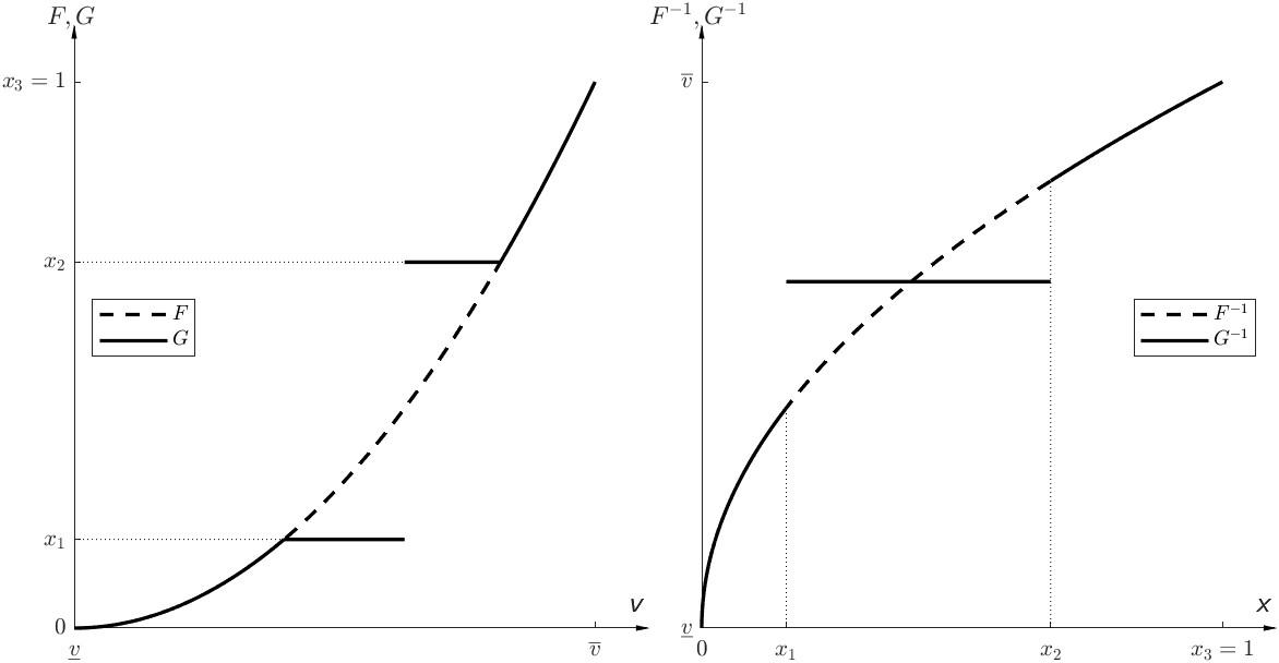
Figure 1: A monotone partitional distribution $G$ which majorizes $F\left(v\right)=v^{2}$. The distribution $G$ has intervals of complete disclosure and of pooled disclosure. The distributions $F,G$ are displayed on the left, the quantile distributions $F^{-1},G^{-1}$ displayed on the right.

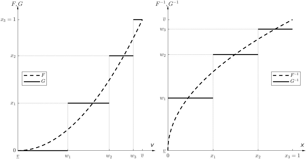
Figure 2: A monotone pooling distribution $G$ which majorizes $F\left(v\right)=v^{2}$ and has only intervals of pooled disclosure. The specific distribution $G$ is the optimal distribution for the quality distribution $Q\left(q\right)=q^{1/4}$.

where $\mathbb{I}_{t\geq\widehat{x}}(t)$ is the indicator function:

$$\mathbb{I}_{t\geq\widehat{x}}(t)\triangleq\begin{cases}1&\text{if }t\geq\widehat{x};\\ 0&\text{if }t<\widehat{x}.\end{cases}$$ (15)

In other words, a weak monotone partitional distribution is generated by first taking all qualities corresponding to quantiles below $\widehat{x}$ and reducing these qualities to zero, and then generating a monotone partitional distribution (where some low qualities have been reduced to 0). A weak monotone pooling distribution is defined in the analogous sense, where all intervals are pooling.

To simplify the exposition, henceforth we omit the qualifier “weak”. Thus, when we say a distribution of qualities $R$ is a monotone partitional (or monotone pooling) distribution $R$, it is always in the weak sense.

We say that $G$ and $R$ have common support if the induced partitions of quantiles that generate the monotone partition distributions are the same. Our first main result establishes that the optimal distributions $G$ and $R$ are monotone pooling distributions.

Theorem 1 (Structure of the Optimal Mechanism)

In every optimal mechanism, $G^{\ast}$ and $R^{\ast}$ are monotone pooling distributions and they have common quantile support.

Here we have to add a qualifying remark. To the extent that some values may not receive a positive quality in the optimal mechanism, there may be some multiplicity in the information structure as represented by $G^{\ast}$. For example, values which do not receive the good (they obtain quality zero) may or may not be pooled. But it is without loss of generality for the optimal mechanism to always pool all values that receive zero quality. Hence, we consider mechanisms $(G,R,\left(q,t\right))$ such that, if $q(w)=q(w^{\prime})=0$ for any pair $w,w^{\prime}\in\mathrm{supp}(G)$, then $w=w^{\prime}$. In other words, all values that are not served with a positive quality are pooled in the same interval of the partition. Of course, this will not change the nature of the optimal mechanism beyond disciplining the information provided to values who do not receive a positive quality.

This first result establishes that every optimal mechanism has monotone pooling information structure. In consequence, the optimal menu will contain only a countable number of items. This contrasts with the continuum of items which would be optimal in the absence of a choice regarding the information structure.

We will prove Theorem 1 in two steps. The first step shows that there exists an optimal mechanism in which the optimal value and quality distributions are monotone partitional. This step shows that given a menu of qualities and prices, the seller’s maximization problem is linear in the quantile function of the expected values. Hence, we can use recent results in klms21 to characterize the optimal information structure in terms of the extreme points of the set of quantile functions that are a mean-preserving spread of the quantile function of values. We then proceed to show that in every optimal mechanism the distributions are partitional. This follows from the fact that the menu and the information structure are jointly optimized. If the information structure were not monotone partitional, then it would be possible to write it as a linear combination of partitional information structures, and each of these would have to be optimal. However, a given vector $q^{\ast}$ cannot be optimal for more than one monotone partitional information structure.

The second step shows that there is no interval of complete information disclosure, and thus the distributions are always monotone pooling. This is the crucial step where we compute the trade-off between information rents and efficiency. We show that for small enough intervals, pooling information and allocations jointly always increases the seller’s profit.

4.1 Monotone Partitional Distribution

The choice of information structure $G$ must be optimal if we hold fixed a distribution $R^{\ast}$ of qualities.  So we consider the problem of choosing $G$ to maximize

$$\Pi=\underset{\{G^{-1}:G^{-1}\prec F^{-1}\}}{\max}\int_{0}^{1}G^{-1}(t)(1-t)dR^{\ast-1}(t).$$ (16)

The optimization problem (16) is an upper semi-continuous linear functional of $G^{-1}$. Upper semi-continuity can be verified by noting that every $G^{-1}\prec F^{-1}$ is upper semi-continuous. Hence, if $\hat{G}^{-1}\rightarrow G^{-1}$ (taking the limit using the $L^{1}$ norm), we have that $\lim\sup\hat{G}^{-1}(t)\leq G^{-1}(t)$ for all $t\in[0,1]$. Hence, $\lim\sup\int_{0}^{1}\hat{G}^{-1}(t)(1-t)dR^{\ast}{}^{-1}(t)\leq\int_{0}^{1}G^{-1}(t)(1-t)dR^{\ast}{}^{-1}(t)$.

Proposition 1 in klms21 shows that the set $\{G^{-1}:G^{-1}\prec F^{-1}\}$ is a convex and compact set, and their Theorem 1 shows that the extreme points of this set are given by (14). Following Bauer’s maximum principle, the maximization problem attains its maximum at an extreme point of $\{G^{-1}:G^{-1}\prec F^{-1}\}$.

The objective function is also linear in $R$, so the same analysis applies. The only difference is that the set of extreme points of the set $\{R^{-1}:R^{-1}\prec_{w}Q^{-1}\}$ is the set of weak partitional structures (see Corollary 2 in klms21). We thus obtain the following result.

Lemma 1 (Sufficiency of Monotone Partitional Distributions)

There exists an optimal mechanism $(G^{\ast},R^{\ast})$ such that $G^{\ast}$ and $R^{\ast}$ are monotone partitional distributions.

We now prove that an optimal mechanism must have a monotone pooling structure. For this, we first prove that, if both distributions have partitional structure, then they must be on a common support (in the quantile space).

Lemma 2 ($G^{\ast}$ and $R^{\ast}$ Have Common Quantile Support)

If $\left(G^{\ast},R^{\ast}\right)$ form an optimal mechanism with monotone partitional distributions, then $G^{\ast}$ and $R^{\ast}$ must have common support.

Proof. We assume that $\left(G,R\right)$ form an optimal mechanism with monotone partitional distributions. We show that $G^{-1}$ is increasing if and only if $R^{-1}$ is, and so they must have a common support.

We first note that, whenever $G^{-1}$ is constant, $R^{-1}$ must also be constant. This follows from the measurability condition $q(w)=R^{-1}(G(w))$. In other words, if there is an atom at some $w$ (so that $G^{-1}$ is constant), all quantiles in the atom must receive the same allocation as these quantiles correspond to the same expected valuation.

Suppose that $R$ is a monotone partition distribution and consider interval $[{x}_{k},{x})$ with $k\not\in J$ (if such interval does not exist, then $R=Q$). We thus have that $R^{-1}(t)$ is constant in $[{x}_{k},{x})$, and $R^{-1}({x}_{k})<R^{-1}({x}_{k+1})$. We show that $G^{-1}(t)$ must also be constant in $[{x}_{k},{x})$.

Suppose $G^{-1}$ is not constant in $[{x}_{k},{x}_{k+1})$, and consider

$$\hat{G}^{-1}(x)\triangleq\begin{cases}G^{-1}(x)&\text{for all }x\not\in[{x}_{k},{x}_{k+1});\\ \frac{\int_{{x}_{k}}^{{x}_{k+1}}G^{-1}(t)dt}{{x}_{k+1}-{x}_{k}}&\text{for all }x\in[{x}_{k},{x}_{k+1}).\end{cases}$$

We obviously have that $G\prec\hat{G}$, so $\hat{G}$ is feasible. Denote the profits generated by mechanisms $(G,R)$ and $(\hat{G},R)$ by $\Pi$ and $\hat{\Pi}$, respectively, and observe that:

$$\Pi-\hat{\Pi}=\bigg{(}(R^{-1}({x}_{k})-R^{-1}({x}_{k}^{-}))(1-{x}_{k})G^{-1}({x}_{k})\bigg{)}-\bigg{(}(R^{-1}({x}_{k})-{R}^{-1}({x}_{k}^{-}))(1-{x}_{k})\hat{G}^{-1}({x}_{k})\bigg{)}.$$

Here $R^{-1}({x}_{k}^{-})$ denotes the left limit of $R^{-1}$ at ${x}_{k}$. Since $G$ is not constant in $[{x}_{k},{x}_{k+1})$ we have that $G^{-1}({x}_{k})<\hat{G}^{-1}({x}_{k})$. We thus conclude that $\Pi-\hat{\Pi}\leq 0$, and the inequality is strict if $R^{-1}({x}_{k})>0$.   

Suppose that there exists an optimal mechanism $(G^{\ast},R^{\ast})$ such that either $G^{\ast}$ or $R^{\ast}$ does not have partitional structure. Then there exists a collection of partitional information structures $\left\{G\right\}$ and a measure $\lambda$ over these partitional structure distributions such that:

$$G^{\ast-1}=\int_{\{G^{-1}:G^{-1}\prec F^{-1}\}}G^{-1}d\lambda(G^{-1}).$$

The same characterization applies for the set of distributions $\{R^{-1}:R^{-1}\prec_{w}Q^{-1}\}$.

Since the functional (13) is linear in $G^{-1}$ and $R^{-1}$, each of these partitional distributions must be optimal. Hence, there must exist two optimal mechanisms $(G_{1}^{\ast},R^{\ast})$ and $(G_{2}^{\ast},R^{\ast})$, with $R^{\ast}$ having partitional structure and $G_{1}^{\ast},G_{2}^{\ast}$ having partitional structure and $G_{1}^{\ast}(w)\neq G_{2}^{\ast}(w)$ for some $w$. However, they cannot both be increasing at a quantile $t$ if and only if $R^{\ast}$ is increasing.

Lemma 3 (Necessity of Monotone Partitional Distribution)

Every optimal mechanism $\left(G^{\ast},R^{\ast}\right)$ has monotone partitional distributions with common support.

The results so far leave open the possibility that there are intervals of complete disclosure.

4.2 Monotone Pooling Distribution

We next show that indeed every interval is a pooling interval in an optimal mechanism. We first provide an intuition and then provide the proof.

Consider a mechanism in which there is full disclosure and full separation in some interval $[v_{1},v_{2}]$ (i.e., $G^{-1}(t)=F^{-1}(t)$ and $R^{-1}(t)=Q^{-1}(t)$ for all $t\in[F(v_{1}),F(v_{2})]$). Suppose the seller pools the allocation of all values in an interval $[v_{1},v_{2}]$, so that all values get the average quality on this interval. How much lower would the profit be? We begin the argument with the virtual values given by:

$$\phi(v)\triangleq v-\frac{1-F(v)}{f(v)}.$$ (17)

The profit generated is the expectation of the product of the virtual values and the qualities:

$$\Pi\triangleq\int_{\underline{v}}^{\bar{v}}q^{\ast}(v)\phi(v)f(v)dv.$$

We denote the (conditional) mean and variance of virtual values and qualities in the interval $[v_{1},v_{2}]$ by:

$${\mu}_{\phi}\triangleq \frac{\int_{v_{1}}^{v_{2}}\phi(v)f(v)dv}{\int_{v_{1}}^{v_{2}}f(v)dv}; \quad{\mu}_{q}\triangleq \frac{\int_{v_{1}}^{v_{2}}q^{\ast}(v)f(v)dv}{\int_{v_{1}}^{v_{2}}f(v)dv};$$ (18)

$$\quad{\sigma}_{\phi}^{2}\triangleq \frac{\int_{v_{1}}^{v_{2}}(\phi(v)-{\mu}_{\phi})^{2}f(v)dv}{\int_{v_{1}}^{v_{2}}f(v)dv}; \quad{\sigma}_{q}^{2}\triangleq \frac{\int_{v_{1}}^{v_{2}}(q^{\ast}(v)-{\mu}_{q})^{2}f(v)dv}{\int_{v_{1}}^{v_{2}}f(v)dv}.$$ (19)

As we only compute conditional mean and variance in the interval $[v_{1},v_{2}]$, we can safely omit an index referring to the interval $\left[v_{1},v_{2}\right]$ in the expression of $\mu$ and $\sigma$. The first step of the proof shows that the revenue losses due to pooling the qualities in the interval $[v_{1},v_{2}]$ are bounded by:

$${\sigma}_{\phi}{\sigma}_{q}(F(v_{2})-F(v_{1})).$$

Hence, pooling the qualities generates third-order profit losses when the interval is small (since each of the terms multiplied are small when the interval is small).

If in addition to pooling the qualities we pool the values in this interval, we can reduce the buyers’ information rent. When only the qualities are pooled–but not the values–then the quality increase that the values which are assigned the pooled quality get relative to values just below the pool is the quality difference $\mu$${}_{q}-q^{\ast}(v_{1})$ priced at $v_{1}$. After pooling the values, the price of the quality increase is computed using the expected value conditional on being in this interval:

$${\mu}_{v}\triangleq\mathbb{E}[v\mid v\in[v_{1},v_{2}]].$$

Hence, pooling the values increases the payments for every value higher than $v_{2}$ by an amount:

$$(\mathbb{E}[v\mid v\in[v_{1},v_{2}]]-v_{1})({\mu}_{q}-{q}^{\ast}(v_{1}))(1-F(v_{1})).$$

Here the first two terms being multiplied are small when the interval is small. However, payments are marginally increased for all values higher than $v_{2}$, which is a non-negligible mass of values (i.e., $(1-F(v_{1}))$ is not small). In other words, pooling values increases the price of the quality improvement $($$\mu$${}_{q}-{q}^{\ast}(v_{1}))$ for all values higher than $v_{2}$. Hence, pooling values generates a second-order benefit which always dominates the third-order distortions.

Lemma 4 (Monotone Pooling Distributions)

The optimal mechanism $\left(G^{\ast},R^{\ast}\right)$ has monotone pooling distributions.

Proof. Following Lemma 1, the optimal information structure consists of intervals of pooling and intervals of full disclosure. We consider an optimal mechanism and an interval $(v_{1},v_{2})$ such that the optimal information structure is full disclosure in this interval (i.e., such that $G^{\ast}(v)=F(v)$). We establish a contradiction by proving that there is an improvement. It is useful to write the interval $(v_{1},v_{2})$ in terms of its mid-point and width:

$$\hat{v}\triangleq\frac{v_{1}+v_{2}}{2};\quad\Delta\triangleq\frac{v_{2}-v_{1}}{2}.$$

So, we have that $(v_{1},v_{2})=(\hat{v}-\Delta,\hat{v}+\Delta)$ and we will eventually take the limit $\Delta\rightarrow 0$.

Following Lemma 2, the qualities $q^{\ast}(v)$ must be strictly increasing in this interval. We consider qualities:

$$\tilde{q}({v})=\begin{cases}{\mu}_{q},&\text{ if ${v}\in({v}_{1},{v}_{2});$}\\ q^{\ast}({v}),&\text{ if ${v}\not\in({v}_{1},{v}_{2}).$}\end{cases}$$

The difference between the optimal policy and the variation is given by:

$$\Pi^{\ast}-\tilde{\Pi}=\int_{{v}_{1}}^{{v}_{2}}\phi(v)q^{\ast}({v})f(v)d{v}-(F(v_{2})-F(v_{1})){\mu}_{\phi}{\mu}_{q}.$$ (20)

Note that we only need to consider the qualities in the interval $[v_{1},v_{2}]$ to compute the difference. We can write this expression more conveniently as follows:

$$\Pi^{\ast}-\tilde{\Pi}=\int_{{v}_{1}}^{{v}_{2}}(\phi(v)-{\mu}_{\phi})(q^{\ast}({v})-{\mu}_{q})f(v)d{v}.$$

Using the Cauchy-Schwarz inequality, we can bound the first integral (and thus the whole expression) as follows:

$$\Pi^{\ast}-\tilde{\Pi}\leq{\sigma}_{q}{\sigma}_{\phi}(F(v_{2})-F(v_{1})).$$ (21)

Finally, using the Bhatia-Davis inequality, we can bound the variances as follows:

$${\sigma}_{q}\leq\sqrt{({\mu}_{q}-q^{\ast}(v_{1}))(q^{\ast}(v_{2})-{\mu}_{q})},$$

and similarly for $\phi$. So we have that:

$$\Pi^{\ast}-\tilde{\Pi}\leq\sqrt{({\mu}_{q}-q^{\ast}(v_{1}))(q^{\ast}(v_{2})-{\mu}_{q})}\sqrt{({\mu}_{\phi}-\phi_{1})(\phi_{2}-{\mu}_{\phi})}(F(v_{2})-F(v_{1})).$$ (22)

We can then conclude that:

$$\lim_{\Delta\rightarrow 0}\frac{\Pi^{\ast}-\tilde{\Pi}}{\Delta^{3}}\leq\frac{dq^{\ast}(\hat{v})}{dv}\frac{d\phi(\hat{v})}{dv}f(\hat{v}).$$ (23)

We thus have that the efficiency losses are of order $\Delta^{3}$.

We now consider the following allocation policy:

$$\hat{q}({v})=\begin{cases}q_{1}^{-},&\text{ if ${v}\in({v}_{1},${$\mu$}${}_{v});$}\\ {\mu}_{q},&\text{ if ${v}\in[${$\mu$}${}_{v},{v}_{2});$}\\ q^{\ast}({v}),&\text{ if ${v}\not\in({v}_{1},v_{2});$}\end{cases}$$ (24)

where

$$q_{1}^{-}\triangleq\lim_{v\uparrow v_{1}}q^{\ast}(v),$$

so the limit is taken from below. We additionally change the information structure so that all values in $({v}_{1},{v}_{2})$ are pooled. That is, the information structure is:

$$\hat{G}({v})=\begin{cases}F({v}_{1}),&\text{ if ${v}\in({v}_{1},${$\mu$}${}_{v});$}\\ F({v}_{2}),&\text{ if ${v}\in[${$\mu$}${}_{v},{v}_{2});$}\\ G(v),&\text{ if ${v}\not\in[v_{1},{v}_{2}).$}\end{cases}$$ (25)

Observe that the total surplus generated by $(\hat{G},\hat{q})$ and by $(G,\tilde{q})$ is the same. Then, the difference in the generated profit is equal to the difference in the expected buyers’ surplus:

$$\hat{\Pi}-\tilde{\Pi}=({\mu}_{q}-q_{1}^{-})({\mu}_{v}-{v}_{1})(1-F(v_{1})).$$ (26)

Since, $q_{1}^{-}\leq q^{\ast}(v_{1})$, we have that:

$$\hat{\Pi}-\tilde{\Pi}\geq({\mu}_{q}-q^{\ast}({v}_{1}))({\mu}_{v}-{v}_{1})(1-F(v_{1})).$$

We conclude that:

$$\lim_{\Delta\rightarrow 0}\frac{\hat{\Pi}-\tilde{\Pi}}{\Delta^{2}}\geq\frac{dq^{\ast}(\hat{v})}{dv}(1-F(v_{1})).$$ (27)

Here we used that $($$\mu$${}_{v}-{v}_{1})/\Delta{\rightarrow}1$, as $\Delta\rightarrow 0.$ The efficiency losses are of order $\Delta^{2}$. We conclude that for $\Delta$ small enough, the new policy generates a profit improvement.   

With Lemma 4 we have therefore completed the proof of Theorem 1. The optimal distributions of values and qualities, $G^{\ast}$ and $R^{\ast}$ are monotone pooling distribution. Furthermore, the corresponding distributions $G^{\ast-1}$ and $R^{\ast-1}$ have common support. Thus, the distributions $G^{\ast}$ and $R^{\ast}$ have the same value in their range as illustrated in Figure 3. More directly, when we plot the quantile distributions $G^{\ast-1}$ and $R^{\ast-1}$ as in Figure 4 then we find that the distributions share the same quantile at which the quantile functions jump upwards. Of course, they can jump to different levels in terms of values and qualities but the jumps occur at the same quantiles which reflects that values and qualities are assorted in monotone manner.

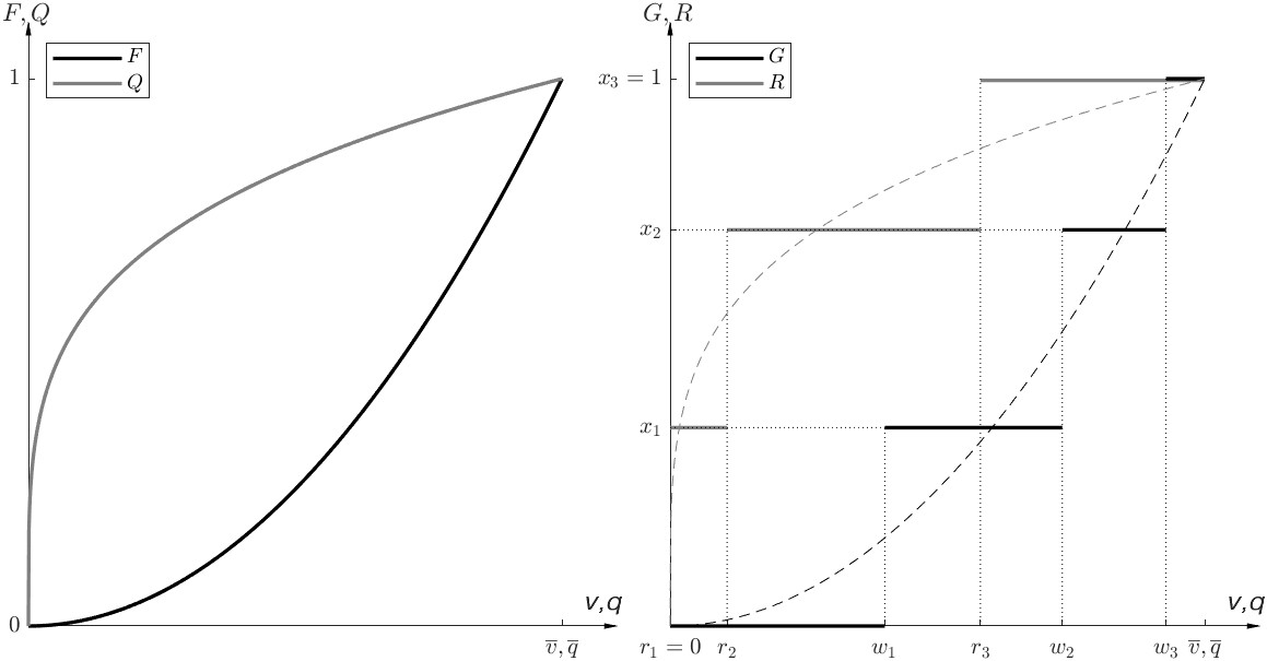
Figure 3: The given distributions of values $F\left(v\right)=v^{2}$ and $Q\left(q\right)=q^{1/4}$ are depicted on the left. The associated optimal distributions $G$ and $R$, which are monotone pooling distributions are depicted on the right.

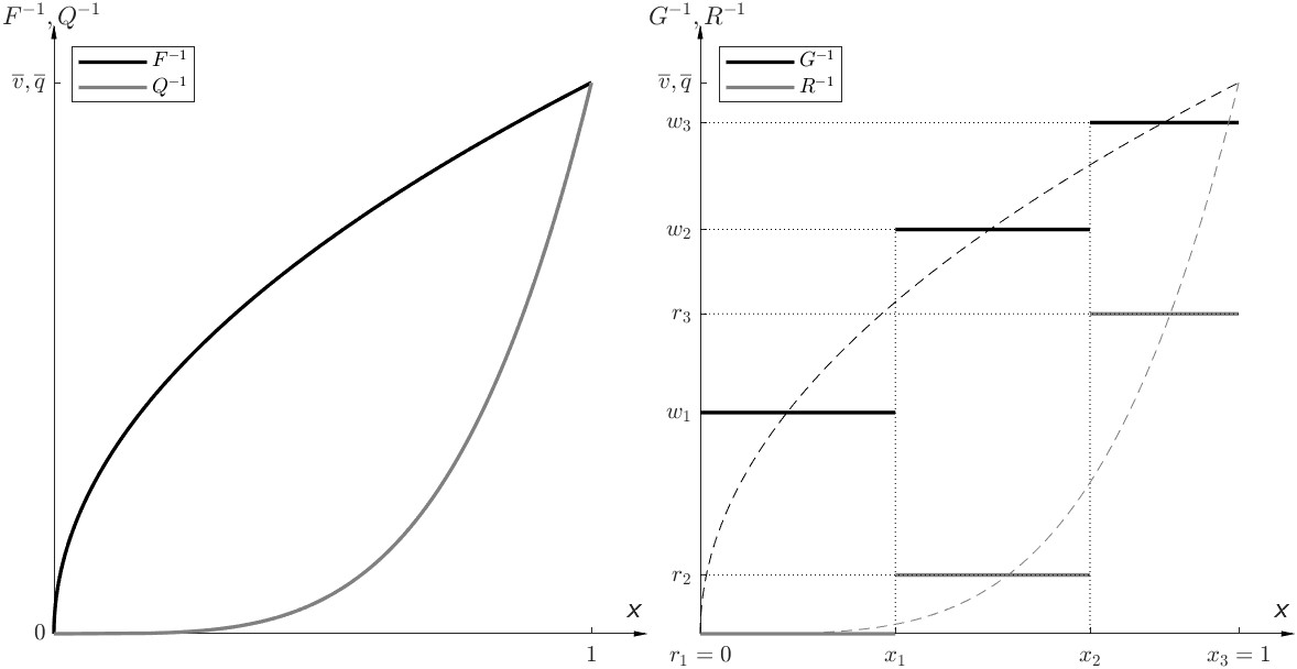
Figure 4: The given quantile distributions $F^{-1}\left(t\right)=t^{1/2}$ and $Q^{-1}\left(t\right)=t^{4}$. The corresponding optimal quantile distributions $G^{-1}$ and $R^{-1}$ have common support and display jumps at the same quantiles.

5 On the Number of Items in the Optimal Menu

So far, we have established that the optimal mechanism pools many values and correspondingly many qualities. The optimal mechanism generates a monotone partition in which each value (and each quality) is bundled with adjacent values (and qualities). The resulting partitions have at most countably many elements. But how many elements will there be in the partition, or correspondingly how many items will there be on the menu? We now establish that there are in fact only finitely many items. Moreover, we provide sufficient conditions to obtain at most $K$ items in the menu, and more refined condition for $K=1$, that is the optimality of a single-item menu.

5.1 The Convexity of Optimal Qualities

We first establish a property of the optimal mechanism that will be important for our results on the size of the menu.  Namely, we show that the optimal menu will have increasing quality increments. This result is of independent interest as it informs us about the structure of the menu independent of the distribution of values. It predicts that in any multi-item menu the distance between any item and its next lower ranked item is increasing as one moves up the quality ladder.

By Theorem 1, the optimal distributions $\left(G^{\ast},R^{\ast}\right)$ are monotone pooling distributions which have common support in the quantile space. Thus, the distribution function $G$ associated with any pooling structure is an increasing and piecewise constant step function $G$. The boundary points of the intervals in the quantile space are denoted by $\left\{x_{k}\right\}_{k\in I}$. The expected values and qualities are denoted by:

$$w_{k}\triangleq\frac{\int_{x_{k-1}}^{x_{k}}F^{-1}(t)dt}{x_{k}-x_{k-1}},\quad r_{k}\triangleq\frac{\int_{x_{k-1}}^{x_{k}}Q^{-1}\left(t\right)\mathbb{I}_{t\geq\widehat{x}}(t)dt}{x_{k}-x_{k-1}},$$

where we recall that $\mathbb{I}_{t\geq\widehat{x}}(t)$ is the indicator function defined earlier in (15). The size of the steps and the distribution at any of these steps is denoted by:

$$G_{k}=G(w_{k}),\quad g_{k}=G(w_{k})-G(w_{k-1}).$$ (28)

These are related to the boundary points of the intervals in the quantile space as follows:

$$G_{k}\triangleq x_{k},\quad g_{k}\triangleq x_{k}-x_{k-1}.$$ (29)

In a finite menu with $K$ items the profit is given by:

$$\Pi=\sum_{k=1}^{K}g_{k}w_{k}r_{k}-\sum_{k=1}^{K}(w_{k+1}-w_{k})r_{k}(1-G_{k}),$$ (30)

where by convention $w_{K+1}\triangleq w_{K}$. This is the discrete counterpart of (12). Finally, the quality increments are denoted by

$$\Delta r_{k}\triangleq r_{k}-r_{k-1},$$ (31)

where we define $r_{0}=0.$ We then express the profit as follows:

$$\Pi=\sum_{k=I}w_{k}\Delta r_{k}(1-G_{k-1}),$$ (32)

where $G_{0}=0.$ This is the discrete counterpart of (13).

Proposition 1 (Increasing Differences in Qualities)

In any optimal mechanism the quality increments $\Delta r_{k}$ must be (weakly) increasing in $k.$

Proof. We fix a mechanism $(G,R)$ and assume that there exists $l$ such that $\Delta r_{l}>\Delta r_{l+1}$. We prove that the mechanism cannot be optimal.

The mechanism is defined as follows. First, for all $k\not\in\{l,l+1\}$, the probabilities, expected values, and qualities remain the same: $\tilde{w}_{k}=w_{k}$, $\tilde{g}_{k}=g_{k}$, $\widetilde{r}(w_{k})=r(w_{k}).$ We modify the information structure as follows:

$$\tilde{g}_{l}= g_{l}+{\varepsilon}\text{;} \quad\tilde{g}_{l+1}= g_{l+1}-{\varepsilon};$$

$$\tilde{w}_{l}= \frac{g_{l}w_{l}+\varepsilon w_{l+1}}{g_{l}+\varepsilon}\text{;} \quad\tilde{w}_{l+1}= w_{l+1};$$

$$r(\tilde{w}_{l})= \frac{g_{l}r(w_{l})+\varepsilon r(w_{l+1})}{g_{l}+\varepsilon}\text{;} \quad\widetilde{r}(\tilde{w}_{l+1})= r(w_{l+1}).$$

Note that:

$$\tilde{g}_{l}\tilde{w}_{l}+\tilde{g}_{l+1}\tilde{w}_{l+1}= g_{l}w_{l}+g_{l+1}w_{l+1};$$

$$\tilde{g}_{l}\widetilde{r}(\tilde{w}_{l})+\tilde{g}_{l+1}\widetilde{r}(\tilde{w}_{l+1})= g_{l}r(w_{l})+g_{l+1}r(w_{l+1});$$

so this is clearly a feasible allocation. The new information structure will not be a partition, but for the purpose of the proof this is irrelevant because we will prove that the stated mechanism is suboptimal. The difference in the profit generated by the original mechanism and the new mechanism are given by:

$$\Pi-\widetilde{\Pi}=w_{l}\Delta r_{l}(1-G_{l-1})+w_{l+1}\Delta r_{l+1}(1-G_{l})-\big{(}\tilde{w}_{l}\Delta\widetilde{r}_{l}(1-\tilde{G}_{l-1})+\tilde{w}_{l+1}\Delta\widetilde{r}_{l+1}(1-\tilde{G}_{l})\big{)}$$

Since $g_{k}=\tilde{g}_{k}$ for all $k\geq l+2$, we can write the difference as follows:

$$\Pi-\widetilde{\Pi}= w_{l}(r(w_{l})-r(w_{l-1}))(1-G_{l+1}+g_{l}+g_{l+1})+w_{l+1}(r(w_{l+1})-r(w_{l}))(1-G_{l+1}+g_{l+1})$$

$$-\big{(}\tilde{w}_{l}(\widetilde{r}(\tilde{w}_{l})-r(w_{l-1}))(1-G_{l+1}+\tilde{g}_{l}+\tilde{g}_{l+1})+\tilde{w}_{l+1}(\widetilde{r}(\tilde{w}_{l+1})-\widetilde{r}(\tilde{w}_{l}))(1-G_{l+1}+\tilde{g}_{l+1})\big{)}$$

Taking the derivative and evaluating at 0, we get:

$$\left.\frac{d(\Pi-\widetilde{\Pi})}{d\varepsilon}\right|_{\varepsilon=0}=-\frac{(1-G_{l-1})(\Delta r_{l+1}-\Delta r_{l})}{g_{l}}.$$

The optimality condition requires this derivative to be less than 0, so we require that $(\Delta r_{l+1}-\Delta r_{l})\geq 0$, which concludes the proof.   

The intuition for the result is that between any two consecutive quality increments levels $\Delta q_{k},$ $\Delta q_{k+1}$, informational rents depend on the lower quality increment level $\Delta q_{k}$ while the surplus gains from separation depend on the higher quality increment level $\Delta q_{k+1}$. To gain a formal intuition for this result, suppose we consider a model with two levels of values and qualities, that is, $v\in\left\{\underline{v},\overline{v}\right\}$, $q\in\{\underline{q},\bar{q}\}$, both uniformly distributed. We ask whether offering a one-item menu via pooling or offering a two-item menu via separating generates higher profit. We also assume excluding the low type is not optimal.

If the items are offered separately, the high value buys the high quality, and the low value buys the low quality. In this environment, the first quality increment is the lower quality level and the second quality increment is the difference between the quality levels:

$$\Delta q_{1}=\underline{q};\quad\Delta q_{2}=\bar{q}-\underline{q}.$$

The total surplus generated when offering a menu is:

$$S_{M}=\frac{1}{2}(\underline{v}\cdot\underline{q}+\bar{v}\cdot\bar{q}).$$

If the goods and values are pooled, the total surplus generated is:

$$S_{P}=\frac{(\bar{v}+\underline{v})}{2}\frac{(\bar{q}+\underline{q})}{2}.$$

The difference is then given by:

$$S_{M}-S_{P}=\frac{1}{4}\Delta q_{2}(\bar{v}-\underline{v}).$$

In contrast, when offering a menu, the informational rents are the rents the high value buyer gains by mimicking the low value buyer:

$$U_{M}=\frac{1}{2}(\bar{v}-\underline{v})\Delta q_{1}.$$

Separating is optimal only when the reduction in informational rents – proportional to $\Delta q_{1}$– is smaller than the surplus gains – proportional to $\Delta q_{2}$. In this example, we get that separating is optimal only if $2\Delta q_{1}\leq\Delta q_{2}$, so the second quality increment must be twice as large as the first quality increment. When doing the variational analysis in the proof, we consider the surplus gains and informational rents reduction when pooling a small fraction of some interval $k+1$ with the immediate predecessor interval $k$. Thus we obtain a weaker condition, namely, increasing differences. However, the intuition is the same: the surplus losses from pooling are proportional to $\Delta q_{k+1}$ while the informational rents reduction are proportional to $\Delta q_{k}$.

The convexity in the qualities provides the key insight to establish that there will be finitely many rather than countable many items. In particular, the convexity of the menu will exclude the possibility of an accumulation point at the top range of the menu.

5.2 Optimality of Finite Item Menu

We can now show that the optimal information structure consists of finitely many signals when $\bar{q}<\infty$.

Theorem 2 (Finite Item Menu)

The optimal mechanism $\left(G^{\ast},R^{\ast}\right)$ is given by finite and monotone pooling distributions.

Proof. Since the space of values is compact, this is equivalent to showing that there are no accumulation points of intervals. We consider three consecutive pooling intervals that generate expected values $w_{k-1}<w_{k}<w_{k+1}$.

Proposition 1 implies that there cannot be any accumulation points, except possibly at some $\hat{v}$ satisfying $q^{\ast}(\hat{v})=0$. Hence, it is a decreasing accumulation point (that is, the limit of expected values converges to $\hat{v}$ from the right). We denote by $\underline{f}$ and $\bar{f}$ the minimum and maximum density in $[\underline{v},(\bar{v}+\hat{v})/2]$:

$$\underline{f}\triangleq\min_{v\in[\underline{v},\frac{(\bar{v}+\hat{v})}{2}]}F^{\prime}(v);\quad\bar{f}\triangleq\max_{v\in[\underline{v},\frac{(\bar{v}+\hat{v})}{2}]}F^{\prime}(v).$$

If such an accumulation point exists, we can find two consecutive pooling intervals, $(v_{k-1},v_{k}]$ and $(v_{k},v_{k+1}]$, generating expected values $w_{k}<w_{k+1}$, satisfying $g_{k}<g_{k+1}$, and:

$$\phi_{k+1}-\phi_{k}<\frac{{\sqrt{\underline{f}}(1-F(v_{k-1}))}}{\sqrt{\bar{f}}(\sqrt{\bar{f}}+\sqrt{\underline{f}})}.$$ (33)

Note that the virtual values $\phi_{k}$ are monotonic, and so we must have that $(\phi_{k+1}-\phi_{k})$ converge to 0 as we take intervals close enough to $\hat{v}$. So, we can take intervals close enough to $\hat{v}$ such that (33) is satisfied. Hence, we consider two intervals satisfying this inequality and reach a contradiction. We recall that the density is not vanishing, so we must have that $\underline{f}>0.$

Analogous to (17), we define:

$$\phi_{k}\triangleq w_{k}-(w_{k+1}-w_{k})\frac{1-G_{k}}{g_{k}},$$

and extend (18)-(19) in the natural way:

$${\mu}_{w}\triangleq\frac{g_{k}w_{k}+g_{k+1}w_{k+1}}{g_{k}+g_{k+1}};\quad{\sigma}_{w}^{2}\triangleq\frac{g_{k}(w_{k}-{\mu}_{w})^{2}+g_{k+1}(w_{k+1}-{\mu}_{w})^{2}}{g_{k}+g_{k+1}}$$

and analogously for $\mu$${}_{q},\$$\sigma$${}_{q},\$$\mu$${}_{\phi},\$$\sigma$_ϕ. Finally, $\hat{\Pi}$ and $\tilde{\Pi}$ are defined in the same way as before. Following the same steps as before, we have that:

$$\frac{\Pi^{\ast}-\tilde{\Pi}}{\hat{\Pi}-\tilde{\Pi}}\leq\frac{\sqrt{({\mu}_{q}-q^{\ast}(w_{k}))(q^{\ast}(w_{k+1})-{\mu}_{q})}\sqrt{({\mu}_{\phi}-\phi_{k})(\phi_{k+1}-{\mu}_{\phi})}(g_{k}+g_{k+1})}{({\mu}_{q}-q^{\ast}({w}_{k}))({\mu}_{w}-{w}_{k})(1-F(v_{k-1}))}.$$

We note that:

$${\mu}_{\phi}-\phi_{k}=\frac{g_{k+1}(\phi_{k+1}-\phi_{k})}{g_{k}+g_{k+1}},\quad\phi_{k+1}-{\mu}_{\phi}=\frac{g_{k}(\phi_{k+1}-\phi_{k})}{g_{k}+g_{k+1}};$$

and the difference between other quantities can be written in an analogous way. We thus get that:

$$\frac{\Pi^{\ast}-\tilde{\Pi}}{\hat{\Pi}-\tilde{\Pi}}\leq\frac{g_{k}(\phi_{k+1}-\phi_{k})(g_{k}+g_{k+1})}{g_{k+1}(w_{k+1}-w_{k})(1-F(v_{k-1}))}.$$

We observe that:

$$g_{k}+g_{k+1}\leq\bar{f}(v_{k+1}-v_{k-1});\quad w_{k}\leq\frac{\sqrt{\bar{f}}v_{k}+\sqrt{\underline{f}}v_{k-1}}{\sqrt{\bar{f}}+\sqrt{\underline{f}}};\quad w_{k+1}\geq\frac{\sqrt{\bar{f}}v_{k}+\sqrt{\underline{f}}v_{k+1}}{\sqrt{\bar{f}}+\sqrt{\underline{f}}}.$$

We finally recall that $g_{k}<g_{k+1}$ so we get that:

$$\frac{\Pi^{\ast}-\tilde{\Pi}}{\hat{\Pi}-\tilde{\Pi}}\leq\frac{\sqrt{\bar{f}}(\phi_{k+1}-\phi_{k})(\sqrt{\bar{f}}+\sqrt{\underline{f}})}{\sqrt{\underline{f}}(1-F(v_{k-1}))}<1,$$

where the second inequality corresponds to (33). Thus, we reach a contradiction with this being an optimal mechanism.   

We assume throughout the analysis that the values and qualities have compact support, in particular that there are finite upper bounds $\bar{q},\bar{v}<\infty$. However, we could relax these conditions. In fact, Theorem 1 remains valid with unbounded supports for values and qualities. For Theorem 2 to remain valid, we can likewise allow for unbounded support of values but do need a bounded support of qualities, thus $\bar{q}<\infty$. With unbounded support for values and qualities countably many items still remain optimal.

5.3 Optimality of Single-Item Menu

We now provide results on the number of items in the optimal menu. We identify a sufficient condition under which it is optimal to offer only a single item. We then provide a general upper bound on the number of items independent of any distributional assumptions.

The first result offers a sufficient condition for the optimal menu to contain a single-item menu.

Theorem 3 (Optimality of Single-Item Menu)

If the distribution $Q\$of qualities has increasing density, then the optimal mechanism is a single-item menu.

Proof. Recall that in a finite-item menu, the profit can be written as in (32). We consider the optimality conditions of the highest two intervals of an optimal mechanism. For this, we define the profit from the highest two items:

$$\Pi_{K-1,K}\triangleq\big{(}(g_{K-1}+g_{K})\Delta r_{K-1}w_{K-1}+g_{K}\Delta r_{K}w_{K}\big{)},$$

which are the last two terms of the summations in (32). If the last two intervals are pooled, then the profit generated would be:

$$\hat{\Pi}_{K-1,K}\triangleq\frac{1}{(g_{K-1}+g_{K})}(g_{K-1}w_{K-1}+g_{K}w_{K})(g_{K-1}r_{K-1}+g_{K}r_{K}-(g_{K-1}+g_{K})r_{K-2}).$$

We now note that:

$$\Pi_{K-1,K}-\hat{\Pi}_{K-1,K}=\frac{(w_{K}-w_{K-1})g_{K}(g_{K-1}(r_{K}-r_{K-1})-(g_{K}+g_{K-1})(r_{K-1}-r_{K-2}))}{g_{K}+g_{K-1}}.$$

To make the expressions more compact, we denote the boundary of the partitions in quality space as follows:

$$q_{K-2}\triangleq Q^{-1}(x_{K-2});\quad q_{K-1}\triangleq Q^{-1}(x_{K-1})$$

and recall that $\bar{q}=Q^{-1}(x_{K})=Q^{-1}(1)$. If the distribution $Q$ has increasing density, then we have that:

$$r_{K-2}\leq q_{K-2};\quad r_{K-1}\geq\frac{q_{K-2}+q_{K-1}}{2};\quad r_{K}\leq\frac{\frac{\bar{q}+q_{K-1}}{2}(\frac{(\bar{q}-q_{K-1})g_{K-1}}{q_{K-1}-q_{K-2}})+\bar{q}(g_{K}-\frac{(\bar{q}-q_{K-1})g_{K-1}}{q_{K-1}-q_{K-2}})}{g_{K}}.$$

The first inequality follows from the fact that $r_{K-2}$ must be smaller than the upper bound of the interval $[q_{k-3},q_{K-2}]$; the second equality follows from the fact that $r_{K-1}$ must be greater than the midpoint of the interval $[q_{K-2},q_{K-1}]$ (since the density is increasing). The third inequality follows from the fact that the density in the last interval $[q_{K-1},\bar{q}]$ is at least $g_{K-1}/(q_{K-1}-q_{K-2})$ so the expected value in the last interval is bounded by the expected value generated by having an atom of size $(g_{K}-\frac{(\bar{q}-q_{K-1})g_{K-1}}{q_{K-1}-q_{K-2}})$ at the top of the support. We thus get that:

$$\Pi_{K-1,K}-\hat{\Pi}_{K-1,K}\leq-\frac{(w_{K}-w_{K-1})(g_{K-1}(\bar{q}-q_{K-1})-g_{K}(q_{K-1}-q_{K-2}))^{2}}{2(g_{K}+g_{K-1})(q_{K-1}-q_{K-2})}<0.$$

Thus, there is an optimal solution in which the last two intervals are pooled. Inductively, we conclude there is always an optimal single-item mechanism. If $\underline{v}>0$ or $q_{K-2}>0$, then the inequality is strict. Note that, if the distribution is uniform, we have that $g_{K}(q_{K-1}-q_{K-2})+g_{K-1}(\bar{q}-q_{K-1})=0$.   

This theorem states that for a large class of distributions $Q$ of qualities the seller will optimally offer a single quality (and a single item) to the buyers. Importantly, the sufficient condition for the distribution of qualities holds for all possible distribution of values. The sufficient condition is tight to the extent that for every distribution $Q$ of qualities that has linear decreasing, but nearly constant density, there exist distribution of values for which a multi-item mechanism is optimal. So even “slightly” decreasing densities can lead to optimal multi-item mechanisms.

A first intuition for the result can be gained by considering a two-item mechanism as follows. Suppose we fix a two-item mechanism, offering low and high qualities to low and high expected value buyers, thus $\left(r_{L},r_{H}\right)$ to $\left(w_{L},w_{H}\right)$ respectively. We then consider the possibility of pooling both items and consequently both values. The benefit of pooling is that the information rents will be eliminated and the cost is that the social surplus will be reduced. However, both of these terms are proportional to the difference in expected values generated by the two-item mechanism. More specifically, the surplus loss is:

$$\Delta S={g_{H}(1-g_{H})}(w_{H}-w_{L})(r_{H}-r_{L}).$$ (34)

If the two items $r_{L}$ and $r_{H}$ are pooled, then the buyers will loose all of their surplus. The reduction in buyers’ surplus is:

$$\Delta U=-g_{H}(w_{H}-w_{L})r_{L}.$$ (35)

In the above two terms, the change in surplus is proportional to the difference in expected values $(w_{H}-w_{L})$. Furthermore, the losses in surplus are smaller than the gains from eliminating buyers surplus when the low quality $r_{L}$ is not too small relative to the high quality $r_{H}$. Note that both expressions are proportional to $(w_{H}-w_{L})$ so the distribution of values does not play a role in the calculation.

When analyzing how to segment a continuous distribution of qualities, we can use the above insights to understand the structure of the optimal policy. If the density of qualities is increasing, then no matter how small the segment is which we try to separate from the lower part of support, the difference in qualities, $r_{H}-r_{L},$ will be small relative to the quality of the lower end of the distribution. In contrast, if the density is decreasing, then by separating a small interval around the top of the value distribution, one can generate a large difference between the low and high quality items.

We can bound the number of items offered in any mechanism. The bound relies on the upper and lower bound of the support of values. For the following result we assume that $\underline{q}>0.$

Proposition 2 (Finite Upper Bound on the Number of Items)

The number of items $K$ offered by an optimal mechanism is bounded above by

$$K\leq\frac{\bar{q}}{\underline{q}}.$$

Proof. The lowest quality item will be at least $r_{1}\geq\underline{q}.$ Using Proposition 1, the $k$-th must have quality of at least $k\underline{q}$. However, the last item, the $K$-th item, cannot have a quality higher than $\bar{q},$ so we have that $K\underline{q}\leq\bar{q}$, which proves the result.   

6 Endogenous Quality Choice

In this section we analyze the model of muro78 where the seller can produce vertically differentiated goods with an increasing and convex cost for quality. Thus, the supply of qualities is endogenous and determined by the seller to maximize profit. We formally introduce the model and show that our earlier results with an exogenous supply of qualities extend to this model with an endogenous supply of qualities. We then provide a novel results that describe how the optimal mechanism changes with the cost function of quality. To understand how the optimal mechanism changes with the cost function, we restrict attention to cost functions with a constant elasticity. We consider the comparative statics of how the cost elasticity impacts the nature of the optimal mechanism and information policy.

6.1 Cost of Quality

We maintain the same environment as described in Section 2 except for the fact that the seller can choose to produce any quality level $q$ at an increasing and convex cost $c(q)$ where $c:\mathbb{R}_{+}\rightarrow\mathbb{R}_{+}$. The seller chooses a menu (or direct mechanism) with qualities $q\left(w\right)$ at prices $p\left(w\right):$

$$M\triangleq\left\{(q(w),p(w))\right\}_{w\in\left[\underline{v},\overline{v}\right]}\text{,}$$

subject to the earlier incentive compatibility and participation constraints, (8) and (9) respectively. The seller’s problem is to maximize expected profit, revenues minus cost:

$$\Pi\triangleq\max_{G,M}\mathbb{E}_{G}[p(w)-c(q(w))].$$

Thus, the only change is that we have added the production cost $c\left(q\right)$. The qualities are now chosen endogenously by the seller rather than given exogenously by the distribution of qualities $Q$.

Following the same steps as in Section 3, we can write the seller’s problem analogous to (13) as follows:

$$\max_{G,R} \int_{0}^{1}G^{-1}(t)(1-t)dR^{-1}(t)-\int_{0}^{1}c(R^{-1}(t))dt,$$ (36)

subject to $$F\prec G R^{-1}$$ and is non-decreasing.

Relative to earlier formulation in (13), we have added the production cost $c\left(q\right)$ and removed the constraint requiring that the quality distribution $R$ must majorize $Q$. Instead we simply require that $R^{-1}$ is non-decreasing in the quantile to satisfy incentive compatibility.

We can verify that Theorem 1 remains valid in this new environment as well. The objective function continues to be linear in $G$. And, in fact, the distribution of expected values $G$ only changes the revenue, but not the expected cost (once we have fixed the allocation rule to be $R$). In the proof of Theorem 1 we showed that the pooling of values always improves the seller’s revenue. Of course, now the pooling of values will also change the cost of the provided qualities. However, if the cost of supplying a given quality is convex, then pooling will reduce the total cost, and so a fortiori the pooling of values remains optimal. We can make this argument precise by showing that for any $R^{-1}\prec_{w}\hat{R}^{-1}$, we have that:

$$\int_{0}^{1}c(R^{-1}(t))dt\leq\int_{0}^{1}c(\hat{R}^{-1}(t))dt.$$ (37)

However, $\hat{R}^{-1}$ is greater than $R^{-1}$ in the increasing convex order if (37) is satisfied for every convex cost $c$ (this is the definition of the increasing convex order; see shsh07 Chapter 4). And, $\hat{R}^{-1}$ is greater than $R^{-1}$ in the increasing convex order if and only if $R^{-1}\prec_{w}\hat{R}^{-1}$ (see Theorem 4.A.3. in shsh07). Thus, starting from any distribution $\hat{R}$ in which there is full disclosure in some interval $[v_{1},v_{2}]$, generating a distribution $R$ that pools values in this interval increases revenue (as shown in Section 4.2). By the convexity of the cost function, this also reduces the cost of providing qualities, thus providing a further benefit to pooling. We obtain the following result.

Theorem 4 (Structure of the Optimal Mechanism)

Given an increasing and convex cost function $c\left(q\right)$, every optimal mechanism $\left(G^{\ast},R^{\ast}\right)$ of (36) displays a finite and monotone pooling distribution.

6.2 Constant Elasticity Cost Function

To understand the role of the cost function $c\left(q\right)$ in the determination of the optimal menu, we now focus on a one-parameter family of cost functions with

$$c\left(q\right)=q^{\eta}/\eta$$

for $\eta>1$.  The parameter $\eta$ represents the (constant) cost elasticity. Note that if costs were linear in quality, i.e., $\eta=1$, then it would be possible for the seller to make infinite profit by offering infinitely large quantities to the buyers.

Consider some fixed information structure $S$ that generates finitely many values $w_{1},...,w_{K}$ each with probability $g_{1},...,g_{K}$ as in (28). We define the corresponding virtual values as:

$$\phi_{k}\triangleq w_{k}-(w_{k+1}-w_{k})\frac{1-G_{k}}{g_{k}}.$$

Without loss of generality we assume that the virtual values $\phi_{k}$ are strictly increasing (since any optimal information structure will satisfy this) and $\phi_{2}>0$ (if $\phi_{1}\leq 0$, there is exclusion on the first interval).

As the cost function is a power function $c(q)=q^{\eta}/\eta$, we can express the profit as a function of the virtual value $\phi$ as follows:

$$\pi(\phi)\triangleq\begin{cases}\frac{\eta-1}{\eta}\phi^{\frac{\eta}{\eta-1}},&\text{if }\phi\geq 0;\\ 0,&\text{otherwise.}\end{cases}$$ (38)

The profit generated by an information structure $S$ is then given by:

$$\Pi_{S}=\sum_{k=1}^{K}g_{k}\pi(\phi_{k}).$$

The profit corresponds to the expected utility that a risk-loving agent obtains when facing a lottery that has payments equal to the virtual values $\{\phi_{k}\}_{k\in K}.$ The relative risk aversion for $\phi\geq 0$ is given by:

$$\frac{\pi^{\prime\prime}(\phi)\phi}{\pi^{\prime}(\phi)}=\frac{1}{\eta-1},$$

so that the hypothetical risk-loving agent is more risk loving as $\eta$ is closer to 1. For comparison, if we were to pool all values $v$ into a single interval with expectation $\mu_{v}=\mathbb{E}\left[v\right]$, then the resulting information structure would generate a profit equal to:

$$\Pi_{P}=\pi(\mu_{v}).$$

We can now compare the profits generated by different information structures.

Proposition 3 (Cost Elasticity and Information Policy)

Consider some finite information structure $S$ with $K>1$ signals:

1. There exists $\overline{\eta}_{S}$ such that information structure $S$ generates less profit than complete pooling if and only if $\eta\geq\overline{\eta}_{S}$.

2. There exists $\underline{\eta}_{S}$ such that information structure $S$ generates less profit than complete disclosure if $\eta\leq\underline{\eta}_{S}$.

Proof. To prove this result, we first compare the profits generated by some finite information structure $S$ and the complete pooling information structure. For this, we note that:

$$\sum_{k\in K}g_{k}\phi_{k}=w_{1}\text{ and }\phi_{K}=w_{K}.$$

We thus have that:

$$\sum_{k\in K}g_{k}\phi_{k}<\mu_{v}\text{ and }\phi_{K}>\mu_{v}.$$

That is, the expectation of the virtual values is strictly less than the expected value, and the highest realization of the virtual values is higher than the expected value of the true values. Following the Arrow-Pratt characterization of risk aversion: a more risk-loving agent (lower $\eta$) always demands a lower certainty equivalent. Furthermore, in the limit $\eta\rightarrow\infty$ the agent becomes risk-neutral, so pooling generates higher profit than $S$. We then conclude that there exists a unique $\overline{\eta}_{S}$ such that:

$$\Pi_{S}\geq\Pi_{P}\iff\eta\geq\overline{\eta}_{S}.$$

This proves the first statement.

We denote by $\hat{\Pi}$ the profit generated by complete disclosure:

$$\hat{\Pi}=\int_{\underline{v}}^{\bar{v}}\pi(\max\{\phi(v),0\})f(v)dv,$$

where $\phi$ is defined in (17). We bound the ratio between the profits generated by $S$ and complete disclosure, respectively, as follows:

$$\frac{\Pi_{S}}{\widehat{\Pi}_{S}}=\frac{\sum_{k=1}^{K}g_{k}\pi(\phi_{k})}{\int_{\underline{v}}^{\bar{v}}\pi(\phi(v))f(v)dv}<\frac{1}{\int_{\phi_{K}}^{\infty}\frac{\pi(\phi(v))}{\pi(\phi_{K})}f(v)dv}.$$

We note that $\phi_{K}<\bar{v}$, and so we have that:

$$\int_{\phi_{K}}^{\infty}f(v)dv>0.$$

We thus have that:

$$\lim_{\eta\rightarrow 1}\frac{\Pi_{S}}{\widehat{\Pi}_{S}}\leq\lim_{\eta\rightarrow 1}\frac{1}{\int_{\phi_{K}}^{\infty}\frac{\pi(\phi(v))}{\pi(\phi_{K})}f(v)dv}=0.$$

The limit is obtained from observing that when $\eta\rightarrow 1$, the exponent in (38) converges to infinity, so the integrand diverges to infinity.   

Proposition 3 considers any given information structure $S$ and evaluates how $S$ performs against either complete pooling or complete disclosure as the cost elasticity changes. For every $S$ there are finite upper and lower bounds , $\overline{\eta}_{S}$ and $\underline{\eta}_{S}$, respectively, such that either complete pooling or complete disclosure dominate the given information structure $S$. Thus, eventually either the suppression of information rent or the social efficiency argument dominate any interior trade-off between these two objectives.

Alternatively, we might consider any given cost function and associated elasticity $\eta$ and ask if the efficiency gains from screening are eventually dominated by the profit gains that come with the suppression of the information rent. In the working paper version, behm22a, we establish as Theorem 5 that if the support of the distribution of values is sufficiently narrow, then the gains from a more efficient allocation are dominated by the reduction in the information rent. Namely, pooling is optimal for every distribution $F$ with support in $\left[\underline{v},\overline{v}\right]$ if and only if

$$\frac{\overline{v}}{\underline{v}}<\eta.$$ (39)

The result is established by a sequence of improvement arguments that terminate with the complete analysis (and explicit solution) of the binary type model. We refer the reader to the working paper for the details of the proof.

There is some earlier work that asks when second-degree price discrimination may optimally resolve in a single-item menu. anda09 impose an a priori finite upper bound on the quality in the setting of muro78. They state conditions under which all values receive the same quality, namely the quality at the upper bound. sand22 shows that their sufficient condition requires that high valuation buyer’s surplus is more concave than that of the low valuation buyer. sand22 shows that a necessary condition for a single-item menu to be profit maximizing is that the single-item menu constitutes the socially optimal allocation. By contrast, in the current environment a continuum of qualities is socially optimal. Hence there would be no reason to restrict the menu and offer a bunching solution in the absence of information design.

7 Discussion and Interpretation

Recommender System as an Indirect Mechanism

Our leading interpretation is that the seller can influence the information that the buyers have about their value but does not observe the realization of the information structure or the value.  Although we did not pursue it formally here, an alternative interpretation of our model is that the seller does in fact observe the buyers’ value but is unable, for regulatory or business reasons, to offer prices for items that depend on the buyers’ value. Thus, the seller cannot engage in perfect price discrimination (or third-degree price discrimination).  In fact, the seller is constrained to offer a menu of items that is common to all buyers.  Yet, as long as all buyers are offered the same menu, the seller is allowed to credibly convey information about buyers’ values.  Now the implementation of the optimal information structure and selling mechanism is that the seller posts a menu and sends a signal to the buyer that recommends one item on the menu.

Formally, the direct mechanism $M$ could also be expressed in terms of a simple indirect menu where the seller chooses $\left(Q,p\right)$ consisting of a set of qualities $Q\subseteq\mathbb{R}_{+}$ and a pricing rule $p:Q\rightarrow\mathbb{R}_{+}$. Then the information structure can be expressed as a recommendation rule $S:\left[\underline{v},\overline{v}\right]\rightarrow\Delta Q$. The resulting recommendation policy is one which we commonly observe on e-commerce platforms. Namely, the seller does not engage in third-degree price discrimination, but rather, among the range of possible choices, every buyer is steered to a specific alternative at a price that is common to all buyers.  This implementation arises in our model if we impose the interim obedience constraint that recommendations are optimal for the buyers conditional on the recommendation received.

Consistent with this interpretation, eBay personalizes the search results for each buyer through a machine learning algorithm and determines a personalized default order of search results in a process referred to as ”Best Match,” see ebay22.  dege19 provide strong evidence that large chains price uniformly across stores despite wide variation in consumer demographics and competition. Further, cava17, (2019) documents that online and offline prices are identical or very similar for large multi-channel retailers, thus confirming the adherence to a uniform price policy. Relatedly, Amazon apologized publicly to its customers when a price testing program offered the same product at different prices to different consumers, and committed to never ”price on consumer demographics,” see amaz00.

Vertical vs. Horizontal Differentiation

We analyzed a canonical model of second-degree price discrimination as in muro78 or mari84. These models largely consider (pure) vertical differentiation among the buyers and in consequence in the choice and price of products. While vertical differentiation captures an important economic aspect, other specifications, in particular horizontal differentiation might be of interest as well. Towards this end, we briefly discuss why horizontal differentiation is likely to lead to very different implications regarding the optimal information policy. Thus, consider a model of pure horizontal differentiation where there are many varieties of the product, and for each type of buyer there is some variety that attains the maximum value and all other varieties generate a lower surplus. Thus for example a utility function $u\left(v,\theta,q\right)=u-\left(v-q\right)^{2}$ would represent such a model of pure horizontal differentiation where the quadratic loss function expresses the fact that for every type $v$, there is an optimal variety, namely $q\left(v\right)=v$, and any deviation leads to a lower utility. In this setting of pure horizontal differentiation, the optimal information policy would be to completely disclose the information about the preferences, and then provide the optimal variety $q^{\ast}\left(v\right)=v$ at a constant price $p^{\ast}=u$ that would indeed extract the efficient social surplus from all values of buyers. This admittedly stark model of pure horizontal differentiation thus leads to a very different information policy than the model of vertical differentiation that we analyzed. For example, movie and tv series recommendation on Netflix and similar streaming services would seem to mirror the implications that a model of horizontal differentiation would predict. By contrast, service level agreements for utilities and telecommunications  or tiered memberships for services would seem to be more directly related to the predictions from the vertical model we analyzed.

Independent Information of the Buyers

In the current analysis, the seller has complete control over how much information beyond the common prior the buyers receive about their value for the products. Frequently, the buyers may have independent sources of information which would allow them to augment and/or substitute the information disclosed by the seller. The second source of information would then impose further constraints on the optimal mechanism as the incentive and participation constraints would have to hold conditional on the information received by the buyer independently from the seller. In the presence of a second source of information, the optimal mechanism may depend on whether the seller is eliciting the private information or not. If the seller were to elicit and incentivize the private information with private and report-dependent offers, then the subsequent analysis would be related to the work of essz07 and lish17. There the seller can extract a large share of surplus due to weaker participation and incentive constraints. By contrast, if the seller would refrain from explicitly eliciting the private information and offer a public and type-contingent recommendations, then we would maintain a public menu of choices as in the current analysis. In earlier work, we referred to these distinct cases as information design with and without elicitation (see bemo19). These joint incentive and information problems are difficult and even in the case of separable information sources as represented by independent random variables and linear objective function, only limited progress has been made so far, see cast21 for a recent contribution.

Beyond the Multiplicative Environment

We stated our main results in the environment of nonlinear pricing first proposed by muro78. There, the buyers’ value is given by a multiplicative separable function of willingness-to-pay and quality, $\theta q$.  The results of Theorem 1 and 2 will continue to hold for any multiplicative separable value function

$$u\left(({v},q,p\right)=h_{v}\left(v\right)h_{q}\left(q\right)-p,$$

where the component functions are increasing in $v$ and $q$ respectively. Moreover, if the utility would be generated by a general supermodular function $h\left(v,q\right)$:

$$u({v},q,p)\triangleq h(v,q)-p,$$

where $h$ is a strictly increasing and supermodular in both arguments $v$ and $q$, then a version of Theorem 1 would still remain to hold. Namely, complete disclosure would never be optimal. However, the pooling of values may no longer be monotone. In the working paper version, behm22a we provide an instance where the optimal information structure is a non-monotone partition. Similarly, in the absence of supermodularity, the finite menu result of Theorem 2 may disappear and in the above we provide an instance where complete disclosure is optimal.

8 Conclusion

In the digital economy, the sellers and the digital intermediaries working on their behalf frequently have a substantial amount of information about the quality of the match between their products and the preferences of the buyers. Motivated by this, we considered a canonical nonlinear pricing problem that gave the seller control over the disclosure of information regarding the value of the buyers for the products offered.

We showed that in the presence of information and mechanism design, the seller offers a menu with only a small number of items. In considering the optimal size of the menu, the seller balances conflicting considerations of efficiency and surplus extraction. The socially optimal menu would provide a menu with a continuum of items to perfectly match quality and taste. By contrast, the profit-maximizing seller seeks to limit the information rent of the buyers by narrowing the choice to a few items on the menu. We provided sufficient conditions for a broad class of distributions under which this logic led the seller to offer only a single item on the menu. While we obtained our results in the model of nonlinear pricing pioneered by muro78, we showed that the coarse menu result remained a robust property in a larger class of nonlinear payoff environments.

In related work, mcaf02 matches two given distributions of, say, consumer demand and electricity supply, and shows how coarse matching by pooling adjacent levels of demand and supply can approximate the socially optimal allocation.  In this analysis, a range of different products are offered in the same class and with the same price. From the perspective of the buyers, the product offered is therefore opaque, as its exact properties are not known to the buyers who is only guaranteed certain distributional properties of the product. This practice is sometimes referred to as opaque pricing, see jian07 and shsh08 for applications to services and transportation and Bergemann et al. (2022) for auctions, in particular for digital advertising. Our analysis regarding the optimality of coarse menus would equally apply if we were to take the distribution of qualities as given and merely determine the partition of the distribution of the qualities. The novelty in our analysis is that the seller renders the preferences of the buyers opaque to find the optimal trade-off between efficient matching of quality and taste against the revenues from surplus extraction.

References

- [1] \harvarditemAnderson \harvardand Dana2009anda09 Anderson, E. \harvardand Dana, J. \harvardyearleft2009\harvardyearright. When is price discrimination profitable, Management Science 55: 980–989.
- [2] \harvarditem[Bergemann et al.]Bergemann, Brooks \harvardand Morris2015bebm15 Bergemann, D., Brooks, B. \harvardand Morris, S. \harvardyearleft2015\harvardyearright. The limits of price discrimination, American Economic Review 105: 921–957.
- [3] \harvarditemBergemann, Heumann \harvardand Morris2022behm22a Bergemann, D., Heumann, T. \harvardand Morris, S. \harvardyearleft2022\harvardyearright. Screening with persuasion, Technical Report 2338, Cowles Foundation for Research in Economics, Yale University.
- [4] \harvarditemBergemann, Heumann, Morris, Sorokin \harvardand Winter2022bhms22 Bergemann, D., Heumann, T., Morris, S., Sorokin, C. \harvardand Winter, E. \harvardyearleft2022\harvardyearright. Optimal information disclosure in classic auctions, American Economic Review: Insights 4: 371–388.
- [5] \harvarditemBergemann \harvardand Morris2019bemo19 Bergemann, D. \harvardand Morris, S. \harvardyearleft2019\harvardyearright. Information design: A unified perspective, Journal of Economic Literature 57: 44–95.
- [6] \harvarditemBergemann \harvardand Pesendorfer2007bepe07 Bergemann, D. \harvardand Pesendorfer, M. \harvardyearleft2007\harvardyearright. Information structures in optimal auctions, Journal of Economic Theory 137: 580–609.
- [7] \harvarditemBlackwell1951blac51 Blackwell, D. \harvardyearleft1951\harvardyearright. Comparison of experiments, Proceedings of the Second Berkeley Symposium in Mathematical Statistics and Probability, University of California Press, Berkeley, pp. 93–102.
- [8] \harvarditemCandogan \harvardand Strackforthcomingcast21 Candogan, O. \harvardand Strack, P. \harvardyearleftforthcoming\harvardyearright. Optimal disclosure of information to a privately informed receiver, Theoretical Economics .
- [9] \harvarditemCavallo2017cava17 Cavallo, A. \harvardyearleft2017\harvardyearright. Are online and offline prices similar? evidence from large multi-channel retailers, American Economic Review 107(1): 283–303.
- [10] \harvarditemCavallo2019cava19 Cavallo, A. \harvardyearleft2019\harvardyearright. More amazon effects: Online competition and pricing behaviors, in F. R. B. of Kansas City (ed.), Jackson Hole Economic Symposium Proceedings, pp. 291–355.
- [11] \harvarditemDellaVigna \harvardand Gentzkow2019dege19 DellaVigna, S. \harvardand Gentzkow, M. \harvardyearleft2019\harvardyearright. Uniform pricing in us retail chains, Quarterly Journal of Economics 134: 2011–2084.
- [12] \harvarditemeBay2022ebay22 eBay \harvardyearleft2022\harvardyearright. Best match, https://tech.ebayinc.com/product/ebay-makes-search-more-efficient-through-personalization/ .
- [13] \harvarditemEső \harvardand Szentes2007essz07 Eső, P. \harvardand Szentes, B. \harvardyearleft2007\harvardyearright. Optimal information disclosure in auctions, Review of Economic Studies 74: 705–731.
- [14] \harvarditemHaghpanah \harvardand Siegel2022hasi22 Haghpanah, N. \harvardand Siegel, R. \harvardyearleft2022\harvardyearright. The limits of multi-product discrimination, American Economic Review: Insights 4: 443–458.
- [15] \harvarditemJiang2007jian07 Jiang, Y. \harvardyearleft2007\harvardyearright. Price discrimination with opaque products, Journal of Revenue and Pricing Management 6: 118–134.
- [16] \harvarditemKamenica \harvardand Gentzkow2011kage11 Kamenica, E. \harvardand Gentzkow, M. \harvardyearleft2011\harvardyearright. Bayesian persuasion, American Economic Review 101: 2590–2615.
- [17] \harvarditem[Kleiner et al.]Kleiner, Moldovanu \harvardand Strack2021klms21 Kleiner, A., Moldovanu, B. \harvardand Strack, P. \harvardyearleft2021\harvardyearright. Extreme points and majorization: Economic applications, Econometrica 89: 1557–1593.
- [18] \harvarditemLi \harvardand Shi2017lish17 Li, H. \harvardand Shi, X. \harvardyearleft2017\harvardyearright. Discriminatory information disclosure, American Economic Review 107: 3363–3385.
- [19] \harvarditemLoertscher \harvardand Muir2022lomu22 Loertscher, S. \harvardand Muir, E. \harvardyearleft2022\harvardyearright. Monopoly pricing, optimal randomization and resale, Journal of Political Economy 130: 566–635.
- [20] \harvarditemMaskin \harvardand Riley1984mari84 Maskin, E. \harvardand Riley, J. \harvardyearleft1984\harvardyearright. Monopoly with incomplete information, RAND Journal of Economics 15: 171–196.
- [21] \harvarditemMcAfee2002mcaf02 McAfee, P. \harvardyearleft2002\harvardyearright. Coarse matching, Econometrica 70: 2025–2034.
- [22] \harvarditemMussa \harvardand Rosen1978muro78 Mussa, M. \harvardand Rosen, S. \harvardyearleft1978\harvardyearright. Monopoly and product quality, Journal of Economic Theory 18: 301–317.
- [23] \harvarditemMyerson1981myer81 Myerson, R. \harvardyearleft1981\harvardyearright. Optimal auction design, Mathematics of Operations Research 6: 58–73.
- [24] \harvarditemRayo2013rayo13 Rayo, L. \harvardyearleft2013\harvardyearright. Monopolistic signal provision, B.E. Journal of Theoretical Economics 13: 27–58.
- [25] \harvarditemRoesler \harvardand Szentes2017rosz17 Roesler, A. \harvardand Szentes, B. \harvardyearleft2017\harvardyearright. Buyer-optimal learning and monopoly pricing, American Economic Review 107: 2072–2080.
- [26] \harvarditemSandmann2022sand22 Sandmann, C. \harvardyearleft2022\harvardyearright. When are single-contract menus profit maximizing?, Technical report.
- [27] \harvarditemShaked \harvardand Shanthikumar2007shsh07 Shaked, M. \harvardand Shanthikumar, J. \harvardyearleft2007\harvardyearright. Stochastic Orders, Springer Verlag.
- [28] \harvarditemShapiro \harvardand Shi2008shsh08 Shapiro, D. \harvardand Shi, X. \harvardyearleft2008\harvardyearright. Market segmentation: The role of opaque travel agencies, Journal of Economics and Management Strategy 17: 803–837.
-
[29]
\harvarditemWeiss2000amaz00
Weiss, T. \harvardyearleft2000\harvardyearright.
Amazon apologizes for price-testing program that angered customers,
Computerworld .
\harvardurlhttps://www.computerworld.com/article/2588337/amazon-apologizes-for-price-testing-program-that-angered-customers.html - [30] \harvarditemWilson1989wils89 Wilson, R. \harvardyearleft1989\harvardyearright. Efficient and competitive rationing, Econometrica 57: 1–40.
- [31]