Multipolar interactions and magnetic excitation gap in d³ spin-orbit Mott insulators

Abstract

In Mott insulators with a half-filled $t_{2g}$ shell the Hund’s rule coupling induces a spin-3/2 orbital-singlet ground state. The spin-orbit interaction is not expected to qualitatively impact low-energy degrees of freedom in such systems. Indeed, $d^{3}$ cubic double perovskites (DP) of heavy transition metals are believed to exhibit conventional collinear magnetic orders. However, their inelastic neutron scattering spectra feature large gaps of unclear origin. Here we derive first-principles low-energy Hamiltonians for the cubic DP Ba₂Y$B^{\prime}$O₆ ($B^{\prime}=$ Os, Ru) and show that they include significant multipolar – dipole-octupolar – intesite exchange terms. These terms break continuous symmetry of the spin-3/2 Hamiltonian opening an excitation gap. The calculated gap magnitudes are in good agreement with experiment. The dipole-octupolar intersite exchange is induced due to excited states of the $t_{2g}^{3}$ manifold that are admixed by the spin-orbit interaction into the spin-3/2 ground state.

I Introduction

Mott insulators of heavy transition metals (TM) exhibit a rich variety of unusual inter-site interactions and ordered phases Witczak-Krempa et al. (2014); Takayama et al. (2021), like Kitaev physics in $d^{5}$ irridates Jackeli and Khaliullin (2009), multipolar orders Chen et al. (2010); Chen and Balents (2011); Lu et al. (2017); Maharaj et al. (2020); Hirai et al. (2020); Paramekanti et al. (2020); Pourovskii et al. (2021); Khaliullin et al. (2021) and valence-bond glasses de Vries et al. (2010); Romhányi et al. (2017) in $d^{1}$ and $d^{2}$ DP, or excitonic magnets in $d^{4}$ perovskites  Jain et al. (2017). These exciting phenomena originate in large spin-orbit (SO) entangling the orbital momentum $L$ with spin $S$ thus splitting the ground state (GS) $LS$ multiplet. The resulting SO GS is then characterized by the total (pseudo-)angular momentum $J_{\mathrm{eff}}$ that depends on the $d$-shell occupancy and determines the space of low-energy local degrees of freedom Takayama et al. (2021).

The physics of $d^{3}$ Mott insulators is expected to be more conventional and less interesting. In the presence of a large octahedral or tetrahedral ligand field, the $t_{2g}$ shell is half-filled. The Hund’s rule thus forces $J_{\mathrm{eff}}=S=3/2$ and $L=$0, i. e. a spin-3/2 orbital singlet GS. The local TM moments are then, to a first approximation, spins-3/2 with their coupling described by a gapless isotropic Heisenberg model. Excited $t_{2g}^{3}$ states are separated by a large Hund’s rule gap Sugano et al. (1970) and perturbatively admixed into the spin-3/2 GS by SO. No remarkable qualitative effects have been theoretically shown to stem from this admixture. In contrast to the exotic orders of the spin-entangled SO Mott insulators, the $d^{3}$ systems usually exhibit conventional antiferromagnetism (AFM). In particular, for a number of $d^{3}$ DP with the formula $A_{2}BB^{\prime}O_{6}$, where $B^{\prime}$ is a heavy magnetic TM, a simple collinear type-I AFM has been inferred from neutron diffraction Battle and Jones (1989); Carlo et al. (2013); Kermarrec et al. (2015); Taylor et al. (2016); Thompson et al. (2016).

All these $d^{3}$ DP systems feature, however, surprisingly ubiquitous large gaps in their inelastic neutron scattering (INS) spectra Carlo et al. (2013); Kermarrec et al. (2015); Taylor et al. (2016); Maharaj et al. (2018); Paddison et al. . The gaps are found in monoclinic DP as well as in the cubic DP Ba₂YOsO₆ (BYOO) and Ba₂YRuO₆ (BYRO). In the monoclinic case, an excitation gap could be explained by a single-ion anisotropy induced by the spin-orbit admixture to the spin-3/2 GS. Its origin is much less clear in the cubic systems, where, for the GS quadruplet, the single-ion anisotropy is negligible Liu et al. (2022), but the measured excitation gap, $\sim$17 meV in BYOO and 5 meV in BYRO Carlo et al. (2013); Kermarrec et al. (2015), is still large. The observed gaps can be fitted by tetragonal single-ion or 2-ion anisotropy terms Taylor et al. (2016); Maharaj et al. (2018), which are, however, not consistent with the absence of any distortions of the cubic symmetry. In all measured systems, the gap is consistently several times larger in the 5$d$ system as compared to its 4$d$ equivalent. In BYOO, a significant SO admixture into the $d^{3}$ GS was confirmed with X-ray scattering by Taylor et al. Taylor et al. (2017). They suggested this admixture to induce the observed excitation gap without providing a concrete physical mechanism relating them.

In this work, we calculate low-energy effective Hamiltonians for BYOO and BYRO in the framework of density functional+dynamical mean-field theory (DFT+DMFT) Georges et al. (1996); Anisimov et al. (1997); Lichtenstein and Katsnelson (1998); Aichhorn et al. (2016) by using an ab initio force-theorem (FT) method Pourovskii (2016). These calculations predict unexpectedly large multipolar – dipole-octupolar (DO) – intersite exchange interactions (IEI) that lift a continuous symmetry of the Hamiltonian thus opening an excitation gap. Our calculation also predict, for both compounds, a non-collinear 2k transverse magnetic order, which is consistent with the propagation vector detected by neutron diffraction. The calculated INS intensities reproduce the experimental spin gap in BYOO as well as its significant reduction in BYRO. These ab initio results are supported by analytical calculations within a simplified tight-binding model predicting leading multipolar IEI to be of the DO type and to scale as a square of SO coupling strength. Overall the present theory provides a consistent explanation for the excitation gaps in cubic $d^{3}$ SO Mott insulators; the same mechanism is shown to enhance the gap in lower symmetry phases.

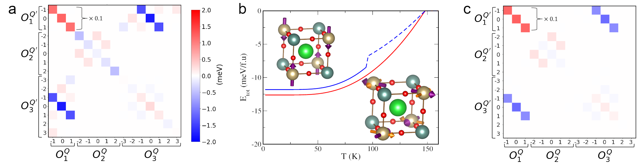
Figure 1: a. Color map of the ab initio IEI matrix $V_{KK^{\prime}}^{QQ^{\prime}}$ for the [1/2,1/2,0] Os-Os pair in BYOO. The dipole-dipole interactions are scaled down by 0.1 in order not to mask other IEI. (b) BYOO mean-field total energy vs. temperature calculated from ab initio $H_{IEI}$ is shown for the 2k-P (lower right corner) and LC (upper left corner) AFM structures by red and blue curves, respectively. In the structure cartoons (plotted by VESTA Momma and Izumi (2011)), the light brown, turquoise, green and small red balls are Os, Y, Ba and O atoms; the directions of dipole and $\Gamma_{5}$ octupole moments are shown by the thick purple and thinner orange arrows, respectively. The first-order discontinuity in the blue curve is a spin-flop transition to the TC AFM ($\textit{{M}}||[110]$); the part of the curve corresponding to this structure is dashed. c. Map of the IEI matrix calculated from the analytical superexchange Hamiltonian. The color scale is the same as in panel a.

The paper is organized as follows. In Sec. II we briefly introduce our ab initio approach (with a detailed description provided in the Appendix). In Sec III we present the ab initio low-energy effective Hamiltonians and analyze their structure; we subsequently discuss the ordered phases and excitation spectra of BYOO and BYRO obtained by solving those Hamiltonains. In Sec. IV we introduce a simplified tight-binding model of $d^{3}$ DP and show how the structure of $t_{2g}$ hopping, in conjunction with the SO coupling, leads to the emergence of the leading multipolar DO IEI.

II Ab initio method

We calculate the electronic structure of BYOO and BYRO using the DFT+DMFT approach of Refs. Blaha et al., 2018; Aichhorn et al., 2009, 2016 treating Ru 4$d$ and Os 5$d$ states within the quasi-atomic Hubbard-I (HI) approximation Hubbard (1963). From the converged DFT+HI electronic structure we calculate all IEI between the $J_{\mathrm{eff}}=3/2$ pseudospins for first several coordination shells using the FT-HI method of Ref. Pourovskii, 2016, analogously to its previous applications to $d^{1}$ and $d^{2}$ DP Fiore Mosca et al. (2021); Pourovskii et al. (2021). Only nearest-neighbor (NN) IEI are found to be important, the next-NN ones are almost two orders of magnitude smaller. See Appendix A.1 for calculational details and Appendix B for the DFT+HI electronic structure of BYOO and BYRO.

III Results

III.1 Low-energy Hamiltonian

IEI between $J_{\mathrm{eff}}=3/2$ GS quadruplets take the following general form

$$H_{IEI}=\sum_{\langle ij\rangle}\sum_{KQK^{\prime}Q^{\prime}}V_{KK^{\prime}}^{QQ^{\prime}}(ij)O_{KQ}^{i}O_{K^{\prime}Q^{\prime}}^{j},$$ (1)

where the on-site multipolar operator $O_{KQ}^{i}$ is the normalized Hermitian spherical tensor Santini et al. (2009) for $J_{\mathrm{eff}}=3/2$ of the rank $K=$1,2,3 (for dipoles, quadrupoles, octupoles, respectively) and projection $Q$ acting on the site at the position $\textit{{R}}_{i}$. These normalized, $\mathrm{Tr}\left[O_{KQ}\cdot O_{K^{\prime}Q^{\prime}}\right]=\delta_{KK^{\prime}}\delta_{QQ^{\prime}}$, tensors are identical, apart from normalization prefactors, to the usual definitions of multipoles in terms of non-normalized polynomials of angular momentum operators, e. g. $O_{10}\equiv O_{z}=J_{z}/\sqrt{5}$, $O_{20}\equiv O_{z^{2}}=\frac{1}{6}(3J_{z}^{2}-J(J+1))$, $O_{30}\equiv O_{z^{3}}=(5J_{z}^{3}-3J(J+1)J_{z}+J_{z})/\sqrt{45}$. The IEI $V_{KK^{\prime}}^{QQ^{\prime}}(ij)$ couples the multipoles $KQ$ and $K^{\prime}Q^{\prime}$ on two magnetic ($B^{\prime}$) sites connected by the lattice vector $\textit{{R}}_{ij}=\textit{{R}}_{j}-\textit{{R}}_{i}$, the first sum is over all NN bonds $\langle ij\rangle$ in the lattice.

The calculated BYOO IEI matrix $\hat{V}(ij)$ for $\textit{{R}}_{ij}=$[1/2,1/2,0] is depicted in Fig. 1a. The leading IEI are diagonal AFM dipole-dipole (DD) terms $V_{11}^{aa}$, where $a=-1,0,1\equiv{y,z,x}$ with an axial anisotropy, $V_{11}^{zz}>V_{11}^{xx(yy)}$.

A striking feature of BYOO $\hat{V}(ij)$ is unexpectedly large DO terms. The leading DO IEI are about 1/8 of the DD ones and ferromagnetic (FM). Other multipolar IEI are at least several times smaller. The picture for BYRO is qualitatively similar to that for BYOO. however, while its DD IEI average of 9.3 meV is close to that in BYOO, both the DD axial anisotropy and DO IEI are an order of magnitude smaller (all calculated IEI for the both systems are listed in Appendix C).

The large DO coupling takes a simple form for the $xy$ bond, $\sum_{Q=-1..1}V_{13}^{QQ}O_{1Q}^{i}O_{3Q}^{j}$, see Fig. 1a, but is less symmetric in the $yz$ and $xz$ planes. We thus introduce the operators $\tilde{O}_{KQ}=O_{KQ}/\langle J_{\mathrm{eff}};3/2|O_{K0}|J_{\mathrm{eff}};3/2\rangle$ to get rid of normalization coefficients in subsequent results and transform the octupole operators into symmetry-adapted octupoles belonging to the $\Gamma_{2}$, $\Gamma_{4}$ and $\Gamma_{5}$ irreducible representations (IREP) Shiina et al. (1997). Keeping only DD and leading DO IEI, one obtains for the $xy$ bond:

$$H^{\prime}_{xy} =V\bm{\tilde{O}}_{1}^{i}\bm{\tilde{O}}_{1}^{j}+\delta V\tilde{O}_{1z}^{i}\tilde{O}_{1z}^{j}+\left[V_{\Gamma_{4}}^{||}\bm{\tilde{O}}_{\Gamma_{4}}^{i}\bm{\tilde{O}}_{1}^{j}-V_{\Gamma_{4}}^{\perp}\tilde{O}_{\Gamma_{4}z}^{i}\tilde{O}_{1z}^{j}\right.$$

$$\left.+V_{\Gamma_{5}}\left(\tilde{O}_{\Gamma_{5}x}^{i}\tilde{O}_{1x}^{j}-\tilde{O}_{\Gamma_{5}y}^{i}\tilde{O}_{1y}^{j}\right)+(i\leftrightarrow j)\right],$$ (2)

where the DO term is in the square brackets, the octupole operators are labeled by the IREP subscript, and $\bm{\tilde{O}}$ are 3D vectors of corresponding operators . Our calculated values for $V$, $\delta V$, $V_{\Gamma_{4}}^{\perp}$, $V_{\Gamma_{4}}^{||}$, and $V_{\Gamma_{5}}$ in BYOO are 5.0, 0.40, 0.39, 0.13, and 0.16 meV, respectively (the formulae for converting the IEI in eq. 1 to those in III.1 are given Appendix C) . $H^{\prime}$ or other bonds are given by cyclic permutation of the indices in (III.1). As we show below, the DO IEI are at the origin of the spin gap in spin-orbit $t_{2g}^{3}$ cubic DP.

III.2 Magnetic order

Subsequently, we employ the calculated ab initio IEI Hamiltonian (Fig. 1a) to derive, within a mean-field (MF) approximation Rotter (2004) , magnetic order as a function of temperature (see Appendix A.2 for relevant methodological details). In the both systems we obtain a planar non-collinear 2k  AFM order (2k-P), depicted in Fig. 1b, as the GS. The dipole (magnetic) moments in 2k-P are $M_{x(y)}=(M/\sqrt{2})\exp[i\textit{{k}}_{y(x)}\textit{{R}}]$, where the propagation vectors k${}_{x}=[1,0,0]$ and k${}_{y}=[0,1,0]$ in the units of $2\pi/a$. The Mdirection thus flips by 90^∘ between adjacent layers. The calculated Néel temperatures, $T_{N}$=146 K in BYOO and 108 K in BYRO, are about twice larger than experimental 69 and 47 K respectively Kermarrec et al. (2015); Carlo et al. (2013); such systematic overestimation by the present MF-based approach was previously observed for other face-centered cubic (fcc) frustrated magnets Pourovskii and Khmelevskyi (2019, 2021); Pourovskii et al. (2021). Another metastable MF solution – a longitudinal collinear type-I AFM structure (LC) with k=[0,0,1] – is found in BYOO at zero temperature to be about 0.8 meV above the 2k-P GS. (Fig. 1b).

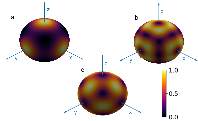
Figure 2: Magnitude of the octupolar $\Gamma_{4}$ and $\Gamma_{5}$ moments as a function of the saturated dipole moment direction $\bm{\hat{M}}=\bm{M}/M$. a). $\Gamma_{4}$ component along $\bm{M}$, $|\langle\bm{\tilde{O}}_{\Gamma_{4}}\rangle\cdot\bm{\hat{M}}|$; b). $\Gamma_{4}$ component orthogonal to M, $|\langle\bm{\tilde{O}}_{\Gamma_{4}}\rangle\times\bm{\hat{M}}|;$ c) $|\langle\bm{\tilde{O}}_{\Gamma_{5}}\rangle|$, $\Gamma_{5}$ octupole is always orthogonal to $\bm{M}$.

Experimentally, a transverse collinear type-I AFM structure (TC) with k=[0,0,1] and moments lying in the $xy$ plane was initially assigned to both BYRO and BYOO by neutron diffraction Battle and Jones (1989); Carlo et al. (2013); Kermarrec et al. (2015), though the exact order type – single-k vs. multi-k – is still debated Fang et al. (2019); Paddison et al. . The predicted GS 2k-P order cannot be distinguished from the TC one on the basis of neutron diffraction only, since the both structures are transverse and feature propagation vectors of the same star. The 1k LC order is not consistent with (100) magnetic Bragg peak observed in the both compounds Carlo et al. (2013); Kermarrec et al. (2015).

One may estimate MF total energies for these competing structures, LC, TC and 2k-P, which are degenerate in an isotropic Heisenberg model, by keeping only the leading anisotropic IEI terms (III.1). Assuming fully saturated dipole moments in all structures, we find the anisotropic contribution to MF total energy (per f.u.) of $2\delta V-4V_{\Gamma_{4}}^{\perp}-4V_{\Gamma_{4}}^{||}$, $-2\delta V+4V_{\Gamma_{4}}^{\perp}-4V_{\Gamma_{4}}^{||}$, $-2\delta V+4V_{\Gamma_{5}}$ and $-2\delta V-8V_{\Gamma_{5}}$ for LC, TC with $\textit{{M}}||$[100], TC with $\textit{{M}}||$[110], and 2k-P, respectively.

The DD IEI alone thus leave TC and 2k-P degenerated, while LC is penalized by the $\delta V$ term due an FM alignment of the out-of-plane moments in the $xy$ plane (Fig. 1b). With the DO terms included, the FM coupling for $\Gamma_{4}$ out-of-plane moments favors, in contrast, the LC order. Finally, the non-collinear 2k-P GS is stabilized by $\Gamma_{5}$ DO coupling. Notice, that the $\Gamma_{5}$ moment is always orthogonal to the saturated dipole one and reaches its maximum for the $\left<110\right>$ dipole-moment direction (see Fig. 2c). Hence, the $\Gamma_{5}$ DO IEI tend to favor $90^{\circ}$ angles between dipole moments that are oriented along $\left<110\right>$. The GS magnetic structure in $d^{3}$ cubic DP is thus determined by a delicate balance between the DD IEI anisotropy and DO coupling.

For the 1k metastable state we obtain a 1st order transition LC$\to$TC at $T\approx 0.65T_{N}$ (Fig. 2b). The difference in MF free-energy between 2k-P and high-$T$ TC is then rather small (see SM sup Sec. III) and may be affected by beyond-MF corrections. One may thus suggest that this TC 1k order sets in at $T_{N}$, with a 1st order transition from TC to 2k-P at lower $T$. Such a 1st-order transition below $T_{N}$ was experimentally observed in the order-parameter evolution of BYOO Kermarrec et al. (2015).

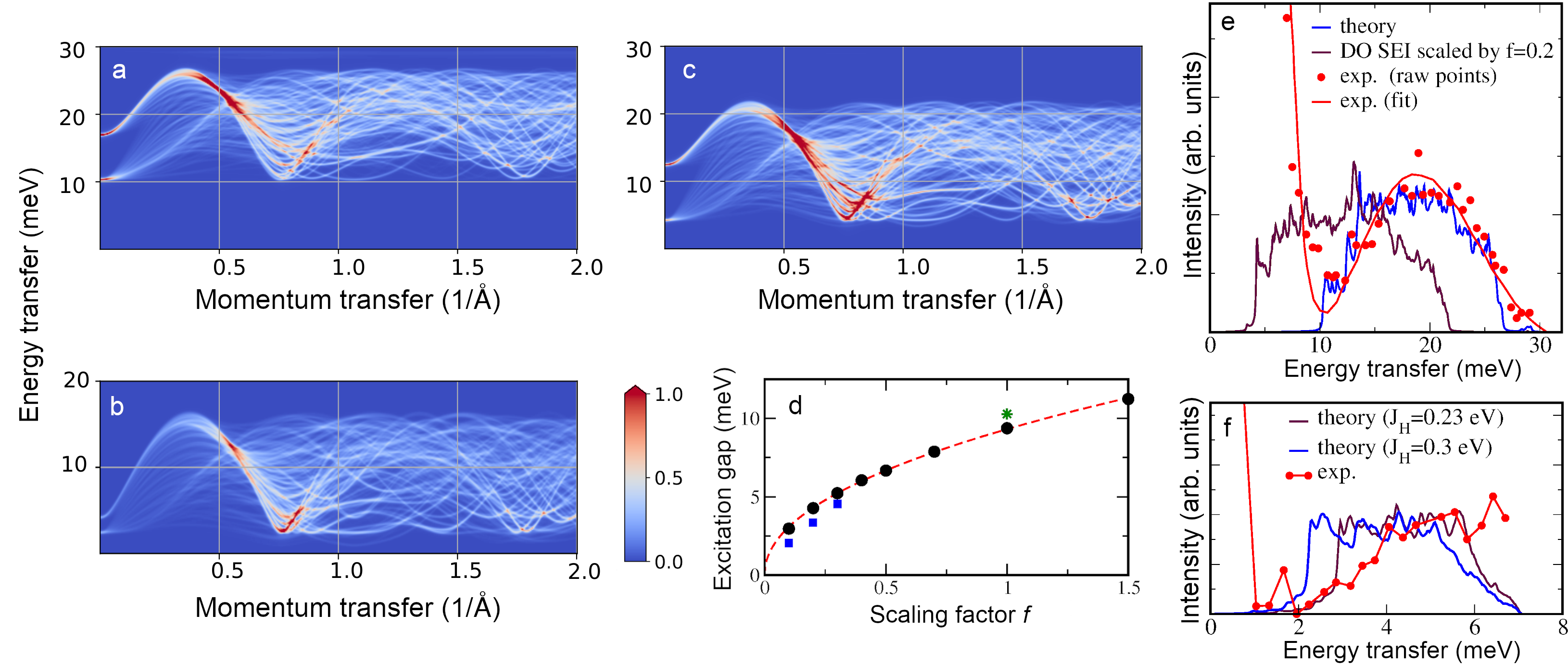
Figure 3: Spherically-averaged INS intensity $S(|\textit{{q}}|,E)$ calculated from the ab initio IEI for a. BYOO; b. BYRO; c. BYOO $S(|\textit{{q}}|,E)$ calculated from the simplified Hamiltonian (III.1) with DO IEI scaled down by $f$=0.2; d. Excitation gap at $|\textit{{q}}|=0.75$ 1/Å as a function of scaling factor $f$ for DO IEI in (III.1). Red dashed line is the $\propto f^{0.48}$ fit to the onset of main spectral weight (circles), the blue squares are the position of a weak resonance appearing at small $f$; the star is the gap value calculated with the full ab initio IEI ; e. Calculated BYOO INS intensity for the initial neutron energy $E_{i}=$120 meV integrated over the $|\textit{{q}}|$ range [0.5:1.5] 1/Å compared to the corresponding experimental data exp from Ref. Kermarrec et al., 2015. f. Calculated BYRO INS intensity for $E_{i}=$11 meV integrated over the $|\textit{{q}}|$ range [0.6:0.9] 1/Å compared to the corresponding experimental data exp from Ref. Carlo et al., 2013.

We note that the DO IEI lift any degeneracy between ordered states that are related by a continuous rotation of dipole moments. The $\Gamma_{4}$ and $\Gamma_{5}$ (as well as $\Gamma_{2}$) octupole moments possess only discrete cubic symmetry. As one sees in Fig. 2, the dipole moment rotation leads to a change in the relative magnitude of associated $\Gamma_{4}$ and $\Gamma_{5}$ octupoles, since they are mixed by any rotation that is not a cubic symmetry operation. Their IE couplings to dipoles (III.1) are distinct and not related by any symmetry in a cubic crystal, therefore, such rotation will change the energy of dipole order. E. g., with only anisotropic DD terms included, the TC $\textit{{k}}=[0,0,1]$ orders are degenerate with respect to a rotation of the ordered moment in the $xy$ plane. With DO IEI (III.1) included, rotating from $\textit{{M}}||[100]$ to $\textit{{M}}||[110]$ induces a $\Gamma_{5}$ octupole and diminishes the $\Gamma_{4}$ one, thus leading to a change in the DO contribution to the ordering energy. This property of DO IEI has profound implications for magnetic excitations, as shown below.

III.3 Magnetic excitations

We calculate the INS intensity $S(\textit{{q}},E)$ of the 2k-P GS using an approach previously applied to $d^{2}$ DP in Ref. Pourovskii et al., 2021. Namely, the dynamical susceptibility $\chi(\textit{{q}},E)$ is calculated in RPA Jensen and Mackintosh (1991) for the MF GS; the zero-temperature INS intensity is then obtained through the fluctuation-dissipation theorem (see, e. g., Ref. Lovesey, 1984) as

$$S(\textit{{q}},E)=\sum_{ab}q^{\perp}_{ab}\\ \sum_{\mu\mu^{\prime}\tau\tau^{\prime}}F_{a\mu}(\textit{{q}})F_{b\mu^{\prime}}(\textit{{q}})\mathrm{Im}\chi_{\mu\mu^{\prime}}^{\tau\tau^{\prime}}(\textit{{q}},E),$$ (3)

where $q^{\perp}_{ab}=\delta_{ab}-\hat{q}_{a}\hat{q}_{b}$, $\tau$ and $\mu\equiv KQ$ label sites in the magnetic unit cell and multipoles, respectively . See Appendix A.3 for further details.

Figure 4: Calculated INS intensity in BYRO integrated around $|\textit{{q}}|$=0.75 Å^-1 (in the range $|\textit{{q}}|$=[0.7275:0.7625] Å^-1) together with the corresponding experimental data from Ref. Paddison et al., . The theoretical curves are calculated for the experimental neutron energy of 11.8 meV and convoluted with a Lorentzian with the width of 0.27 meV corresponding to the experimental instrumental resolution. The experimental error bars are estimated from Fig. 4b of Ref. Paddison et al., .

The spherically-averaged INS intensities $S(|\textit{{q}}|,E)$ for BYOO and BYRO calculated in the 2k-P GS structure using the ab initio IEI exhibit a clear excitation gap (Figs. 3a and 3b). In Figs. 3e and 3f we compare our theoretical $|\textit{{q}}|$-integrated INS intensities with experimental low-temperature ones  Kermarrec et al. (2015); Carlo et al. (2013) employing the same $|\textit{{q}}|$-integration ranges as in those works . We find a nearly perfect quantitative agreement for BYOO.

The excitation gap is somewhat underestimated in BYRO with Hund’s rule coupling $J_{H}=0.3$ eV that we adopted for both compounds; using smaller $J_{H}$=0.23 eV we obtain a good agreement for the gap. In Fig. 4 we compare the INS intensity for BYRO integrated around $|\textit{{q}}|$=0.75 Å^-1 with very recent experimental data from Ref. Paddison et al., . The comparison is displayed for two choices of $J_{H}$, 0.3 eV and 0.23 eV. One observes a rather good agreement with experiment, which is overall better for the smaller $J_{H}$ value. The excitation gap is seen to be enhanced with decreasing $J_{H}$ due to the corresponding enhancement of the DO IEI as $\sim(\lambda/J_{H})^{2}$, where $\lambda$ is the SO coupling parameter, see Sec. IV below.

Thus the experimental picture – of a large excitation gap in these cubic DP with its magnitude being several times larger in BYOO as compared to BYRO – is fully reproduced by the present theory. We note that the position of low-energy intensity peak in the vicinity of the (100) Bragg reflection, $|\textit{{q}}|=$0.75 Å^-1, is also reproduced in both compounds; the high-energy intensity peak at $|\textit{{q}}|$ about 0.5 Å^-1 is outside of the experimental range in Refs. Kermarrec et al., 2015; Carlo et al., 2013.

The origin of this excitation gap is DO IEI, which break continuous rotation symmetry of the intersite exchange Hamiltonian, leading to disappearance of Goldstone modes. To demonstrate this explicitly, we employ the simplified Hamiltonian $H^{\prime}$ (III.1) of BYOO with the DO IEI scaled by a factor $f$. The 2k-P GS is stable in the $f$ range we explore. At $f$=1 the gap value calculated with $H^{\prime}$ is very close to that obtained with the full Hamiltonian (1), see Fig. 3d. With $f$=0.2, the gap is reduced to about 4 meV as compared to $\approx$10 meV at $f$=1 (Fig 3c and Fig 3e). We carried out this calculation for a set of $f$ values; the resulting gap magnitude (Fig. 3d) exhibits a power dependence $\propto f^{\alpha}$, where $\alpha\approx 0.5$. A very weak resonance also appears below the onset of main spectral weight at $f<$0.5, see SM sup Sec. VI for details. With the gap scaling as a square-root of the DO IEI strength $f$ and the latter behaving as $f\sim(\lambda/J_{H})^{2}$, one finds $\sim 1/J_{H}$ dependence for the gap; this agrees with the numerical results for BYRO displayed in Fig. 4.

IV Dipole-octupolar intersite exchange in a tight-binding model

In order to clarify the origin of large DO IEI terms, in this section we derive superexchange interactions in a simplified tight-binding model relevant for the SO DP.

We start with analyzing the impact of SO on the GS of a $t_{2g}^{3}$ shell. In the absence of SO, the Hund’s rule coupling splits 20 states of the $t_{2g}^{3}$ manifold into 3 energy levels, which are the GS ${}^{4}A_{2}$ quadruplet, 10 degenerate levels belonging to a ${}^{2}E$ quadruplet and a ${}^{2}T_{1}$ sextet, and an upper ${}^{2}T_{2}$ sextet. The energies of two excited levels are 3$J_{\mathrm{H}}$ and 5$J_{\mathrm{H}}$, respectively, with respect to the GS Sugano et al. (1970). All these wave functions are listed as Slater determinants in Ref. Sugano et al., 1970. Introducing the notation $x,y,z\equiv yz,xz,xy$ for the $t_{2g}$ orbitals, one may write the ${}^{2}T_{2}$ states in the second-quantization notation as

$$|^{2}T_{2}(x);1/2\rangle=\frac{1}{\sqrt{2}}\left(y_{\downarrow}^{\dagger}z_{\uparrow}-z_{\downarrow}^{\dagger}y_{\uparrow}\right)|{}^{4}A_{2};3/2\rangle,$$

$$|^{2}T_{2}(y);1/2\rangle=\frac{1}{\sqrt{2}}\left(z_{\downarrow}^{\dagger}x_{\uparrow}-x_{\downarrow}^{\dagger}z_{\uparrow}\right)|{}^{4}A_{2};3/2\rangle,$$ (4)

$$|^{2}T_{2}(z);1/2\rangle=\frac{1}{\sqrt{2}}\left(x_{\downarrow}^{\dagger}y_{\uparrow}-y_{\downarrow}^{\dagger}x_{\uparrow}\right)|{}^{4}A_{2};3/2\rangle,$$

where $\left|{}^{2}T_{2}(a);1/2\right\rangle$ are the ${}^{2}T_{2}$ wavefunctions for the orbital projection $a=x,y,z$ and spin projection $M=\frac{1}{2}$; $|^{4}A_{2};3/2\rangle$ is the wavefuntion of the GS quadruplet with $M=\frac{3}{2}$. We also introduced the corresponding creation/annihilation operators for each one-electron orbital $x$, $y$, $z$ and spin.

The SO operator for the $t_{2g}$ shell is $-\lambda\sum_{i}\bm{l}_{i}\bm{s}_{i}$, where the SO coupling parameter $\lambda>0$. The spin-off-diagonal (spin lowering) part of this operator reads

$$-\frac{\lambda}{2}l_{+}s_{-}=\frac{\lambda}{2}\left[(x_{\downarrow}^{\dagger}z_{\uparrow}-z_{\downarrow}^{\dagger}x_{\uparrow})+i(y_{\downarrow}^{\dagger}z_{\uparrow}-z_{\downarrow}^{\dagger}y_{\uparrow})\right],$$

where $s_{-/+}(l_{-/+})$ is the spin(pseudo-orbital) lowering/raising ladder operator.

Hence, one sees that in the 1st-order perturbation theory (PT), the SO coupling admixes ${}^{2}T_{2}$ states to the pseudo-spin quadruplet, leading to the following expression for the $M=\frac{3}{2}$ state:

$$\left|J_{\mathrm{eff}};\frac{3}{2}\right\rangle= \left|{}^{4}A_{2},\frac{3}{2}\right\rangle+$$

$$\frac{\epsilon_{\mathrm{SO}}}{\sqrt{2}}\left(\left|{}^{2}T_{2}(y);\frac{1}{2}\right\rangle-i\left|{}^{2}T_{2}(x);\frac{1}{2}\right\rangle\right),$$ (5)

where $\epsilon_{\mathrm{SO}}=\lambda/(5J_{\mathrm{H}})$. Other $J_{\mathrm{eff}}=3/2$ quartet states are obtained from (IV) by a successive application of the $j_{-}=s_{-}-l_{-}$ operator.

By directly diagonalizing the self-consistent DFT+HI $t_{2g}$ Os atomic Hamiltonian, we obtain the GS state with the largest SO admixture from ${}^{2}T_{2}$, but also non-negligible contributions of two other IREP. Hence, other excited levels, which contribute in the 2nd-order PT ($\sim\epsilon_{\mathrm{SO}}^{2}$), also admix non-negligibly to the $J_{\mathrm{eff}}=3/2$ GS. The normalized GS quadruplet states read

$$\left|J_{\mathrm{eff}};M\right\rangle=\sum_{R\in\mathrm{IREP}}C[R]\left|R;M\right\rangle,$$ (6)

where $C[R]$ is the total contribution due to a given IREP $R$. With the numerical diagonalization (in which the ab initio value of $\lambda$=0.294 eV), we obtain the exited level admixtures $C[^{2}E]$=0.052, $C[^{2}T_{1}]$=0.063, and $C[^{2}T_{2}]$=0.220, compared to the 1st-order PT result shown above, with only $C[^{2}T_{2}]=\left(1+\epsilon_{\mathrm{SO}}^{-2}\right)^{-1/2}=$0.192 being non-zero. Our magnitudes for the admixture of excited $t_{2g}^{3}$ levels to the Os 5d³ GS agree well with estimations from RIXS measurements Taylor et al. (2017). As shown below, the 2nd-order ${}^{2}E_{g}$ contribution to the GS is crucial for the DO IEI.

Subsequently, we employ the GS wavefunctions (6) to calculate BYOO superexchange (SE) analytically within a simplified tight-binding model for the hopping. We assume the hopping $H_{12}$ between Os $t_{2g}$ shells 1 and 2 that are connected by the R=[1/2,1/2,0] fcc lattice vector to be given by $\sum_{\sigma}t^{\prime}\left(x^{\dagger}_{1\sigma}y_{2\sigma}+x^{\dagger}_{2\sigma}y_{1\sigma}\right)-tz^{\dagger}_{1\sigma}z_{2\sigma}+h.c.$, see, e. g., Ref. Takayama et al., 2021. The hopping $t$ between the orbitals ($z$) that lie in the bond plane is dominating, $t>t^{\prime}$. We further simplify analytical calculations by assuming the same energy for all two-site atomic excitations, $E_{0}($d²d${}^{4})=\bar{U}$. Though the latter approximation is rather crude quantitatively, it does not affect qualitative conclusions with respect to the origin of multipolar IEI. The model SE Hamiltonian is then given by $H_{\mathrm{SE}}=-H_{12}^{2}/\bar{U}=H_{t^{\prime}t^{\prime}}+H_{tt}+H_{tt^{\prime}}$, where the three terms in RHS arise due to the hopping involving only out-of-plane ($x$,$y$) orbitals ($t^{\prime}t^{\prime}$) , only in-plane ($z$) orbitals ($tt$) and their mixture ($tt^{\prime}$). Omitting unimportant single-site contributions, $H_{t^{\prime}t^{\prime}}$ and $H_{tt}$ read

$$H_{t^{\prime}t^{\prime}}= \frac{2(t^{\prime})^{2}}{\bar{U}}\sum_{\begin{subarray}{c}\sigma\sigma^{\prime}\\ a=x,y\end{subarray}}\left[(a_{2\sigma}^{\dagger}a_{2\sigma^{\prime}})(\bar{a}_{1\sigma^{\prime}}^{\dagger}\bar{a}_{1\sigma})\right.+$$

$$\left.(\bar{a}_{2\sigma}^{\dagger}a_{2\sigma^{\prime}})(\bar{a}_{1\sigma^{\prime}}^{\dagger}a_{1\sigma})\right],$$ (7)

$$H_{tt}=\frac{2t^{2}}{\bar{U}}\left[\sum_{\sigma\sigma^{\prime}}(z^{\dagger}_{2\sigma}z_{2\sigma^{\prime}})(z^{\dagger}_{1\sigma^{\prime}}z_{1\sigma})\right],$$ (8)

where $\bar{x}=y$, $\bar{y}=x$. All the terms in $H_{tt}$ an $H_{t^{\prime}t^{\prime}}$ are seen to have the same general structure, $X_{1}X_{2}$, where both onsite operators $X$ in a given term are of the same type (i. e., spin and orbital diagonal, either spin or orbital off-diagonal, both spin and orbital off-diagonal). The mixed term $H_{tt^{\prime}}$ does not contribute to leading multipolar IEI in the $J_{\mathrm{eff}}=3/2$ space.

We then calculate all $J_{\mathrm{eff}}=3/2$ SE matrix elements $\langle M_{1}^{1};M_{2}^{2}|H_{\mathrm{SE}}|M_{3}^{1};M_{4}^{2}\rangle$, where the superscript of $M$ is the site label, and convert them to the coupling $V_{KK^{\prime}}^{QQ^{\prime}}(\textit{{R}})$ between on-site moments using eq. 11.

In the zeroth order in $\epsilon_{\mathrm{SO}}$, i. e. $\left|J_{\mathrm{eff}};M\right\rangle=\left|{}^{4}A_{2},M\right\rangle$, one obtains an isotropic AFM Heisenberg coupling between spins-3/2, $5J\sum_{Q=x,y,z}O_{1Q}(1)O_{1Q}(2)\equiv J\vec{S}_{1}\vec{S}_{2}$, where $J=(4t^{2}+8(t^{\prime})^{2})/9\bar{U}$.

In order to evaluate the relative importance of SO-admixed excited states for the SE, we calculate the SE matrix elements with the corresponding wavefunctions $\left|R;M\right\rangle$. The largest non-vanishing SE contributions stemming from the SO admixtures are of $O(\epsilon_{\mathrm{SO}}^{2})$. They are of the types $\langle{}^{4}A_{2}^{1};{}^{2}E^{2}|H_{SO}|{}^{4}A_{2}^{1};{}^{4}A_{2}^{2}\rangle$ and $\langle{}^{4}A_{2}^{1};{}^{2}T_{2}^{2}|H_{SO}|{}^{4}A_{2}^{1};{}^{2}T_{2}^{2}\rangle$, where we omit the $M$ quantum number for brevity. (Note that matrix elements of the type $\langle{}^{4}A_{2}^{1};{}^{2}T_{2}^{2}|H_{SO}|{}^{4}A_{2}^{1};{}^{4}A_{2}^{2}\rangle$, which would contribute in $O(\epsilon_{\mathrm{SO}})$, are all zero, since a non-zero matrix element $\langle{}^{4}A_{2}|X_{1}|{}^{2}T_{2}\rangle\langle{}^{4}A_{2}|X_{2}|{}^{4}A_{2}\rangle$ requires orbitally off-diagonal $X_{1}$ and orbitally diagonal $X_{2}$.) The largest $O(\epsilon_{\mathrm{SO}}^{2})$ terms are due to $H_{tt}$; they contribute to DO and anisotropic DD IEI.

The fact that SE contributions like

$$\langle{}^{4}A_{2}^{1};{}^{2}E^{2}|H_{tt}|{}^{4}A_{2}^{1};{}^{4}A_{2}^{2}\rangle\propto$$

$$\sum_{\sigma\sigma^{\prime}}\langle{}^{4}A_{2}|z^{\dagger}_{\sigma}z_{\sigma^{\prime}}|{}^{4}A_{2}\rangle\langle{}^{2}E|z^{\dagger}_{\sigma^{\prime}}z_{\sigma}|{}^{4}A_{2}\rangle,$$ (9)

map within the $J_{\mathrm{eff}}=3/2$ space into a DO coupling can be shown explicitly by expanding those on-site matrices into multipole moments. Namely, with the magnetic quantum number written explicitly, those $4\times 4$ matrices are $X^{AA}_{MM^{\prime}}(\sigma\sigma^{\prime})=\langle^{4}A_{2};M|z^{\dagger}_{\sigma}z_{\sigma^{\prime}}|^{4}A_{2};M^{\prime}\rangle$ and $X^{EA}_{MM^{\prime}}(\sigma^{\prime}\sigma)=\langle^{2}E;M|z^{\dagger}_{\sigma^{\prime}}z_{\sigma}|^{4}A_{2};M^{\prime}\rangle$. By expanding them as $X=\sum_{KQ}\mathrm{Tr}[X\cdot O_{KQ}]O_{KQ}$ one finds that the $X^{AA}$ matrices map only to dipole moments, as expected. In contrast, the $X^{EA}$ ones map, apart from dipoles, also to octupoles and quadrupoles. The contribution of the latter (which would result in a symmetry-forbidden dipole-quadrupole interaction) is canceled out between Hermitian-conjugated terms in $H_{tt}$, hence, only DD and DO SE terms remain. A similar analysis is applicable for the second $\sim\epsilon_{\mathrm{SO}}^{2}$ contribution, $\langle^{4}A_{2};^{2}T_{2}|H_{\mathrm{SO}}|^{4}A_{2};^{2}T_{2}\rangle$, since the matrices $X^{TT}_{MM^{\prime}}(\sigma\sigma^{\prime})=\langle^{2}T_{2};M|z^{\dagger}_{\sigma}z_{\sigma^{\prime}}|^{2}T_{2};M^{\prime}\rangle$ also map into dipoles and octupoles.

The corresponding matrix elements of $H_{t^{\prime}t^{\prime}}$ also contribute in $O(\epsilon_{\mathrm{SO}}^{2})$ to both the DO and anisotropic DD couplings, as well as to quadrupole-quadrupole (QQ) ones; these contributions are smaller by the hopping anisotropy factor $(t^{\prime}/t)^{2}$ as compared to the $H_{tt}$ ones. Hence, this analysis confirms that in $t_{2g}^{3}$ SO double perovskites, the DO couplings are expected to be the largest IEI besides the conventional DD ones.

Employing a reasonable set of parameters ($t=$0.1 eV and $t^{\prime}=0.3t$, $\bar{U}=$2 eV) in and the ab initio GS wavefunctions (6) in the simplified model described above, we obtain the IEI matrix $\hat{V}$ (Fig. 1c) that is in a good qualitative agreement with the ab initio one (Fig. 1a). The contribution due to the ${}^{2}E$ admixture is dominant determining an axial anisotropy of DD IEI with $V_{zz}>V_{xx}=V_{yy}$ (the ${}^{2}T_{2}$ contribution favors a planar anisotropy). The DO IEI are ferro-coupled pairs of the corresponding moments with $Q=$ -1,0,1(=$y,z,x$); they are an order of magnitude smaller than DD IEI. The QQ and octupole-octupole terms are insignificant.

V Summary and Outlook

In summary, our ab initio calculations of the low-energy effective Hamiltonians in the $d^{3}$ spin-orbit double perovskites Ba₂YOsO₆ and Ba₂YRuO₆ predict significant multipolar intersite exchange interactions (IEI). Such significant multipolar IEI are quite unexpected in the case a half-filled $t_{2g}^{3}$ shell. The leading multipolar IEI are of a dipole-octupole (DO) type. Namely, they couple the conventional total angular-moment operators $J_{a}$ ($a=x,y,z$) acting on a magnetic site (Os or Ru) with octopolar operators, which are time-odd cubic polynomials of $J_{a}$, acting on its nearest-neighbor magnetic sites. The DO IEI lift continuous symmetry of the effective Hamiltonian resulting in a gaped excitation spectra. The multipolar IEI are thus at the origin of the large excitation gaps that were previously observed in inelastic neutron scattering spectra (INS) of $d^{3}$ spin-orbit double perovskites Carlo et al. (2013); Kermarrec et al. (2015); Paddison et al. . The theoretical INS spectra calculated from the effective Hamiltonians are in a good quantitative agreement with those measurements. These ab initio results are further supported by analysis in the framework of a simplified analytical model, which predicts the DO terms to be leading IEI, besides the conventional Heisenberg terms, in $d^{3}$ cubic double perovskites. Usually, bi-quadratic (quadrupole-quadrupole) IEI $\sim\left(J_{a}^{i}J_{a^{\prime}}^{j}\right)^{2}$ are assumed to be the most significant multipolar IEI in such $d^{3}$ systemsFang et al. (2019); Paddison et al. . Our results contradict this assumption. Moreover, the DO IEI are also predicted to stabilize a non-collinear $2\textit{{k}}$ transverse structure, which propagation vector $\textit{{k}}=\langle 1,0,0\rangle$ agrees with experimentCarlo et al. (2013); Kermarrec et al. (2015) .

On the basis of our analysis, the leading dipole-octupolar IEI are expected to scale as $(\lambda/J_{H})^{2}$, where $\lambda$ is the spin-orbit coupling strength and $J_{H}$ is the Hund’s rule coupling. Since $J_{H}$ is weakly changing along the 4$d$ and 5$d$ TM series and between them, the dipole-octupolar IEI magnitude $f$ is effectively controlled by $\lambda^{2}$. The numerical RPA calculations for the excitation gap vs. $f$ (Fig. 3d) find that the gap scales as $\sqrt{f}\propto\lambda$ thus explaining the fact that the measured gap in $5d$ systems is several times larger compared to that in equi-electronic $4d$ systems.

Moreover, the DO IEI can also be expected to provide a major contribution to the excitation gap in non-cubic spin-orbit d³ Mott insulators. To estimate this contribution, we have also evaluated for Ba₂YOsO₆ the excitation gap in the LC magnetic structure (shown in Fig. 1b) stabilized by 1% of tetragonal compression (see SM sup Sec. IV for details). A tetragonal compression $\epsilon_{t}>$0.5% is predicted by our calculations to stabilize it against 2k-P due to an easy-axis single-site anisotropy. With yet larger compression, $\epsilon_{t}=$1%, the LC structure is stable even with DO IEI put to zero. Calculating the LC excitation spectra of this tetragonal structure with and without the DO IEI block, we find that the DO IEI double the magnitude of the excitation gap. This confirms that the effect of DO IEI on the gap is still significant even in systems with a large single-ion anisotropy.

Appendix A Methodological details

A.1 Ab initio calculations

Our DFT+HI calculations are based on the full-potential LAPW code Wien2kBlaha et al. (2018) and include the SO interaction with the standard second-variation approach. Projective Wannier orbitals Amadon et al. (2008); Aichhorn et al. (2009) representing Os (Ru) $d$ orbitals are constructed from the Kohn-Sham (KS) bands in the energy range [-1.4:4.8] ([-1.4:4.1]) eV relative to the KS Fermi level; this energy window includes all $t_{2g}$ and most of $e_{g}$ states but not the oxygen 2$p$ bands (see SMsup for plots of the KS density of states in BYOO and BYRO).

A rotationally invariant Coulomb vertex for the full $d$ shell is constructed using the parameters $U^{d}=F^{0}$ and $J^{d}_{H}=(F^{2}+F^{4})/14$ together with the standard additional approximationAnisimov et al. (1993) for the ratio of Slater parameters $F^{4}/F^{2}=$0.625. Some test calculations for BYOO were carried out using ”small window” including only Os $t_{2g}$ states and the Kanamori rotationally invariant $t_{2g}$ Hamiltonian with the corresponding parameters $U=U^{d}+8J_{H}^{d}/5$ and $J_{H}=0.77J_{H}^{d}$. In all calculations of BYOO, unless specified otherwise, we employ $F^{0}=U^{d}=2.6$ eV and Hund’s rule $J_{H}^{d}=0.39$ eV. For the $t_{2g}$ Kanamori Hamiltonian they correspond to $U=$3.05 eV, which is within the accepted range for 5$d$ DP Erickson et al. (2007); Romhányi et al. (2017); Fiore Mosca et al. (2021), and $J_{H}$=0.30 eV inferred for BYOO from measurements in Ref. Taylor et al., 2017. For BYRO, unless noted otherwise, we employ the same value of $J_{H}$ as in BYOO and the larger value of $U^{d}=$3.6 eV to account for a stronger localization of 4$d$ states.

All calculations are carried out for the experimental cubic lattice structures of BYRO Aharen et al. (2009) and BYOO Kermarrec et al. (2015). We employ the local density approximation as the DFT exchange-correlation potential, 400 k-points in the full Brillouin zone, and the Wien2k basis cutoff $R_{\mathrm{mt}}K_{\mathrm{max}}=$8. The double-counting correction is evaluated using the fully-localized limit with the nominal $d$ shell occupancy of 3. Extensive benchmarks demonstrate the robustness of our qualitative results with respect to varying $J_{H}$ , (see Fig. 4), DFT calculational parameters, double-counting correction or employing the $t_{2g}$ Hamiltonian instead of the full $d$-shell, see SMsup Sec. II.

Calculations of IEI $V_{KK^{\prime}}^{QQ^{\prime}}(ij)$ acting within the $J_{\mathrm{eff}}=3/2$ space are carried out using the FT-HI approach of Ref. Pourovskii, 2016, analogously to previous applications of this method to actinide dioxides Pourovskii and Khmelevskyi (2019, 2021) as well as to d¹ and ² double perovskites Fiore Mosca et al. (2021); Pourovskii et al. (2021). This approach is similar to other magnetic force theorem methods for symmetry-broken phases (Refs. Liechtenstein et al., 1987; Katsnelson and Lichtenstein, 2000, see also Ref. Szilva et al., for a recent review) but is formulated for the paramagnetic state. Within the FT-HI, the matrix elements of IEI $V(ij)$ coupling $J_{\mathrm{eff}}=3/2$ quadruplets on two $B^{\prime}$ sites read

$$\langle M_{1}M_{3}|V(ij)|M_{2}M_{4}\rangle=\mathrm{Tr}\left[G_{\langle ij\rangle}\frac{\delta\Sigma^{at}_{j}}{\delta\rho^{M_{3}M_{4}}_{j}}G_{\langle ji\rangle}\frac{\delta\Sigma^{at}_{i}}{\delta\rho^{M_{1}M_{2}}_{i}}\right],$$ (10)

where $<ij>\equiv\textit{{R}}_{j}-\textit{{R}}_{i}$ is the lattice vector connecting the two sites, $M=-3/2,...,3/2$ is the magnetic quantum number, $\rho^{M_{1}M_{2}}_{i}$ is the corresponding element of the $J_{\mathrm{eff}}$-quadruplet density matrix on site $i$, $\frac{\delta\Sigma^{at}_{i}}{\delta\rho^{M_{1}M_{2}}_{i}}$ is the derivative of atomic (Hubbard-I) self-energy $\Sigma^{at}_{i}$ over a fluctuation of the $\rho^{M_{1}M_{1}}_{i}$ element, $G_{\langle ij\rangle}$ is the inter-site Green’s function. The self-energy derivatives are calculated from atomic Green’s functions using analytical formulas derived in Ref. Pourovskii, 2016, where the FT-HI method is described in detail. The method is applied as a post-processing on top of DFT+HI, hence, all quantities in the RHS of eq. 10 are evaluated from a fully converged DFT+HI electronic structure.

Once all matrix elements (10) are calculated, we make use of the orthonormality property $\mathrm{Tr}\left[O_{KQ}\cdot O_{K^{\prime}Q^{\prime}}\right]=\delta_{KK^{\prime}}\delta_{QQ^{\prime}}$ of the Hermitian multipolar operators $O_{KQ}$ (which are defined in accordance with eq. 10 of Ref. Santini et al., 2009) to map them into the IEI $V_{KK^{\prime}}^{QQ^{\prime}}(ij)$ between on-site moments:

$$V^{QQ^{\prime}}_{KK^{\prime}}(ij)=$$ (11)

$$\sum_{\begin{subarray}{c}M_{1}M_{2}\\ M_{3}M_{4}\end{subarray}}\langle M_{1}M_{3}|V(ij)|M_{2}M_{4}\rangle\left[O_{KQ}\right]_{M_{2}M_{1}}\left[O_{K^{\prime}Q^{\prime}}\right]_{M_{4}M_{3}}.$$

To have a correct mapping into the $J_{\mathrm{eff}}$ pseudo-spin basis, the phases of the $|J_{\mathrm{eff}};M\rangle$ states are chosen such that $\langle J_{\mathrm{eff}};M|J_{+}|J_{\mathrm{eff}};M-1\rangle$ is a positive real number.

A.2 Mean-field (MF) solution of the effective Hamiltonian

We employ the MCPHASE package Rotter (2004) in conjunction with an in-house module implementing multipolar operators in the MCPHASE framework to solve the effective Hamiltonian $H_{IEI}$ in mean-field. As initial guesses of the MF procedure we employ all 1k  structures realizable within single fcc unit cell; these calculations converge to the 2k-P order. In order to obtain a metastable 1k solution we start with the corresponding initial guess switching off the random Monte Carlo flips implemented in the MCPHASE. With this procedure the LC structure is obtained at low $T$ independently of whether it or the TC one is used as the initial guess.

A.3 Inelastic neutron scattering (INS) intensities

We evaluated the generalized dynamical susceptibility $\chi(\textit{{q}},E)$ for the MF ground state using a generalized random phase approximation (RPA), see Ref. Jensen and Mackintosh, 1991. The INS intensity is calculated from $\chi(\textit{{q}},E)$ by eq. 3 using the form-factors $F_{a\mu}(\textit{{q}})$ for $J_{\mathrm{eff}}=3/2$ multipole $\mu\equiv{KQ}$, where $a=x,y,z$. Our approach for evaluating these form-factors is based on analytical expressions for the one-electron neutron scattering operator $Q_{a}(\textit{{q}})$ from Ref. Lovesey, 1984, which matrix elements in the $d^{3}$ $J_{\mathrm{eff}}$ space are calculated with the HI eigenstates of the $J_{\mathrm{eff}}=3/2$ quadruplet. The resulting matrices are then expanded in multipole operatorsShiina et al. (2007) as

$$\langle J_{\mathrm{eff}};M|Q_{a}(\textit{{q}})|J_{\mathrm{eff}};M^{\prime}\rangle=\sum_{\mu}F_{a\mu}(\textit{{q}})\left[O_{\mu}\right]_{MM^{\prime}}$$

to obtain the form factors.

The method is described in detail in Supp. Material of Ref. Pourovskii et al., 2021. The radial integrals $\langle j_{L}(q)\rangle$ for the Os⁵⁺ 5$d$ shell, which enter into the formulas for one-electron matrix elements of $Q_{a}(\textit{{q}})$, were taken from Ref. Kobayashi et al., 2011. For Ru⁵⁺, the full set of $\langle j_{L}(q)\rangle$ has not been given in the literature, to our awareness. We thus use an estimate for Ru⁵⁺ $\langle j_{0}(q)\rangle$ from Ref. Parkinson et al., 2003; for $L=2,4$ we assume the same values of $\langle j_{L}(q)\rangle$ as in Os⁵⁺.

The spherically averaged INS intensities $S(|\textit{{q}}|,E)$ are calculated for each $|\textit{{q}}|$ by averaging over 642 q-points on an equidistributed icosahedral mesh.

Appendix B Electronic structure of BYOO and BYRO

The IEI calculations by the FT-HI method were carried out starting from the converged DFT+HI electronic structure of BYOO and BYRO.

Figure 5: DFT+HI spectral function of BYOO (a) and BYRO (b). The partial $t_{2g}$ spectral function is shaded in red.

In Fig. 5 we display the converged DFT+HI spectral functions of the both compounds obtained with the full-$d$ correlated subspace . Both systems are predicted by DFT+HI to be correlated insulators with the gap of about 2.4 eV and 1.9 eV in BYOO and BYRO respectively. The insulating gap in BYOO is between the Os $t_{2g}$ lower and upper Hubbard bands (HB), hence, this compound is predicted to be a Mott insulator. In contrast, BYRO is a charge-transfer insulator, since the gap is between the upper edge of O 2$p$ valence band and the Ru upper HB. DFT+HI predictions for the gap magnitude are not expected to be quantitatively accurate, since the HB width is known to be underestimated in this approximation Kotliar et al. (2006) leading to the gap being overestimated as noted, e. g., in the case of rare-earth sesquioxides Boust et al. (2022). There are no published experimental data on the gap magnitude or transport in BYOO and BYRO, to our awareness. The DFT+HI electronic structure compares qualitatively well with previous DFT-based calculations (which used somewhat different parameters). In particular, Refs. Wang et al., 2019; Fang et al., 2019 also predicted a Mott gap in BYOO to open between $t_{2g}$ HB, though those calculations had to be made in a magnetically ordered phase due to the well-known limitation of standard DFT(+U) methods in capturing local-moment paramagnetism. They employed smaller values of U, correspondingly, their calculated gap was also smaller than the one we find. Ref. Chen, 2018 employing DFT+U and DFT+DMFT predicted both paramagnetic and antiferromagnetic BYRO to be insulating for the values of $U$ and $J_{H}$ employed in the present work.

For the sake of reproducibility, we also plot the auxiliary non-interacting Kohn-Sham densities of states of BYOO and BYRO in SMsup Sec. I.

Appendix C Intersite exchange interactions

In Table 1 we list all calculated IEI in BYOO and BYRO with magnitude above 0.05 meV. The IEI are given for the [0.5,0.5,0.0] nearest-neighbor fcc lattice vector.

We also list below the formulas to convert these IEI into the IEI of the simplified Hamiltonain (eq. III.1):

$$V=\frac{9}{20}V_{11}^{11},$$ (12)

$$\delta V=\frac{9}{20}(V_{11}^{00}-V_{11}^{11}),$$ (13)

$$V_{\Gamma_{4}}^{\perp}=-\frac{3}{20}\left(V_{13}^{00}+\sqrt{\frac{3}{8}}V_{13}^{11}\right),$$ (14)

$$V_{\Gamma_{4}}^{||}=-\frac{3}{20}\sqrt{\frac{3}{8}}V_{13}^{11},$$ (15)

$$V_{\Gamma_{5}}=-\frac{3}{20}\sqrt{\frac{5}{8}}V_{13}^{11},$$ (16)

where the overall prefactors (9/20 and 3/20) are due to the change of operators normalization from $O$ to $\tilde{O}$, and the square-root factors are due to the transformation to the cubic IREP.

Table 1: Calculated IEI $V_{KK^{\prime}}^{QQ^{\prime}}$. First two columns list $Q$ and $Q^{\prime}$ , respectively. Third and fourth columncolumns list Cartesian labels for the $KQ$ and $K^{\prime}Q^{\prime}$ tensors. The last three columns display the values of all IEI for BYOO and BYRO (meV) with magnitude above 0.05 meV (for BYRO we list IEI calculated using two values of $J_{H}$).

				BYOO	BYRO	BYRO
				$J_{H}$= 0.3 eV	0.3 eV	0.23 eV
Dipole-Dipole
-1	-1	y	y	11.22	9.27	9.67
0	0	z	z	12.12	9.34	9.79
1	1	x	x	11.22	9.27	9.67
Dipole-Octupole
-1	-1	y	yz2	-1.38	-0.11	-0.17
-1	1	y	xz2	0.10
-1	3	y	x(3x2-y2)	0.16
0	-2	z	xyz	0.21
0	0	z	z3	-1.78	-0.13	-0.21
1	-3	x	y(x2-3y2)	-0.16
1	-1	x	yz2	0.10
1	1	x	xz2	-1.38	-0.11	-0.17
Quadrupole-Quadrupole
-2	-2	xy	xy	-0.50
-1	-1	yz	yz	-0.22
0	-2	z2	xy	0.23
0	0	z2	z2	-0.10
1	-1	xz	yz	0.19
1	1	xz	xz	-0.22
2	2	x2-y2	x2-y2	-0.51
Octupole-Octupole
-2	-2	xyz	xyz	-0.07
-1	-1	yz2	yz2	0.16
0	-2	z3	xyz	-0.06
0	0	z3	z3	0.28
1	-1	xz2	yz2	-0.06
1	1	xz2	xz2	0.16
2	2	z(x2-y2)	z(x2-y2)	-0.09

References

- Witczak-Krempa et al. (2014) W. Witczak-Krempa, G. Chen, Y. B. Kim, and L. Balents, Annual Review of Condensed Matter Physics 5, 57 (2014).
- Takayama et al. (2021) T. Takayama, J. Chaloupka, A. Smerald, G. Khaliullin, and H. Takagi, Journal of the Physical Society of Japan 90, 062001 (2021).
- Jackeli and Khaliullin (2009) G. Jackeli and G. Khaliullin, Phys. Rev. Lett. 102, 017205 (2009).
- Chen et al. (2010) G. Chen, R. Pereira, and L. Balents, Phys. Rev. B 82, 174440 (2010).
- Chen and Balents (2011) G. Chen and L. Balents, Phys. Rev. B 84, 094420 (2011).
- Lu et al. (2017) L. Lu, M. Song, W. Liu, A. P. Reyes, P. Kuhns, H. O. Lee, I. R. Fisher, and V. F. Mitrovic, Nature Communications 8, 14407 (2017).
- Maharaj et al. (2020) D. D. Maharaj, G. Sala, M. B. Stone, E. Kermarrec, C. Ritter, F. Fauth, C. A. Marjerrison, J. E. Greedan, A. Paramekanti, and B. D. Gaulin, Phys. Rev. Lett. 124, 087206 (2020).
- Hirai et al. (2020) D. Hirai, H. Sagayama, S. Gao, H. Ohsumi, G. Chen, T.-h. Arima, and Z. Hiroi, Phys. Rev. Research 2, 022063(R) (2020).
- Paramekanti et al. (2020) A. Paramekanti, D. D. Maharaj, and B. D. Gaulin, Phys. Rev. B 101, 054439 (2020).
- Pourovskii et al. (2021) L. V. Pourovskii, D. F. Mosca, and C. Franchini, Phys. Rev. Lett. 127, 237201 (2021).
- Khaliullin et al. (2021) G. Khaliullin, D. Churchill, P. P. Stavropoulos, and H.-Y. Kee, Phys. Rev. Research 3, 033163 (2021).
- de Vries et al. (2010) M. A. de Vries, A. C. Mclaughlin, and J.-W. G. Bos, Phys. Rev. Lett. 104, 177202 (2010).
- Romhányi et al. (2017) J. Romhányi, L. Balents, and G. Jackeli, Phys. Rev. Lett. 118, 217202 (2017).
- Jain et al. (2017) A. Jain, M. Krautloher, J. Porras, G. H. Ryu, D. P. Chen, D. L. Abernathy, J. T. Park, A. Ivanov, J. Chaloupka, G. Khaliullin, B. Keimer, and B. J. Kim, Nature Physics 13, 633 (2017).
- Sugano et al. (1970) S. Sugano, Y. Tanabe, and H. Kamimura, Multiplets of Transition-Metal Ions in Crystals (Academic Press, New York, 1970).
- Battle and Jones (1989) P. Battle and C. Jones, Journal of Solid State Chemistry 78, 108 (1989).
- Carlo et al. (2013) J. P. Carlo, J. P. Clancy, K. Fritsch, C. A. Marjerrison, G. E. Granroth, J. E. Greedan, H. A. Dabkowska, and B. D. Gaulin, Phys. Rev. B 88, 024418 (2013).
- Kermarrec et al. (2015) E. Kermarrec, C. A. Marjerrison, C. M. Thompson, D. D. Maharaj, K. Levin, S. Kroeker, G. E. Granroth, R. Flacau, Z. Yamani, J. E. Greedan, and B. D. Gaulin, Phys. Rev. B 91, 075133 (2015).
- Taylor et al. (2016) A. E. Taylor, R. Morrow, R. S. Fishman, S. Calder, A. I. Kolesnikov, M. D. Lumsden, P. M. Woodward, and A. D. Christianson, Phys. Rev. B 93, 220408(R) (2016).
- Thompson et al. (2016) C. M. Thompson, C. A. Marjerrison, A. Z. Sharma, C. R. Wiebe, D. D. Maharaj, G. Sala, R. Flacau, A. M. Hallas, Y. Cai, B. D. Gaulin, G. M. Luke, and J. E. Greedan, Phys. Rev. B 93, 014431 (2016).
- Maharaj et al. (2018) D. D. Maharaj, G. Sala, C. A. Marjerrison, M. B. Stone, J. E. Greedan, and B. D. Gaulin, Phys. Rev. B 98, 104434 (2018).
- (22) J. A. M. Paddison, H. Zhang, J. Yan, M. J. Cliffe, S.-H. Do, S. Gao, M. B. Stone, D. Dahlbom, K. Barros, C. D. Batista, and A. D. Christianson, arXiv:2301.11395 (unpublished).
- Liu et al. (2022) X. Liu, D. Churchill, and H.-Y. Kee, Phys. Rev. B 106, 035122 (2022).
- Taylor et al. (2017) A. E. Taylor, S. Calder, R. Morrow, H. L. Feng, M. H. Upton, M. D. Lumsden, K. Yamaura, P. M. Woodward, and A. D. Christianson, Phys. Rev. Lett. 118, 207202 (2017).
- Georges et al. (1996) A. Georges, G. Kotliar, W. Krauth, and M. J. Rozenberg, Rev. Mod. Phys. 68, 13 (1996).
- Anisimov et al. (1997) V. I. Anisimov, A. I. Poteryaev, M. A. Korotin, A. O. Anokhin, and G. Kotliar, Journal of Physics: Condensed Matter 9, 7359 (1997).
- Lichtenstein and Katsnelson (1998) A. I. Lichtenstein and M. I. Katsnelson, Phys. Rev. B 57, 6884 (1998).
- Aichhorn et al. (2016) M. Aichhorn, L. Pourovskii, P. Seth, V. Vildosola, M. Zingl, O. E. Peil, X. Deng, J. Mravlje, G. J. Kraberger, C. Martins, et al., Computer Physics Communications 204, 200 (2016).
- Pourovskii (2016) L. V. Pourovskii, Phys. Rev. B 94, 115117 (2016).
- Momma and Izumi (2011) K. Momma and F. Izumi, Journal of Applied Crystallography 44, 1272 (2011).
- Blaha et al. (2018) P. Blaha, K. Schwarz, G. Madsen, D. Kvasnicka, J. Luitz, R. Laskowski, F. Tran, and L. D. Marks, WIEN2k, An augmented Plane Wave + Local Orbitals Program for Calculating Crystal Properties (Karlheinz Schwarz, Techn. Universität Wien, Austria,ISBN 3-9501031-1-2, 2018).
- Aichhorn et al. (2009) M. Aichhorn, L. Pourovskii, V. Vildosola, M. Ferrero, O. Parcollet, T. Miyake, A. Georges, and S. Biermann, Phys. Rev. B 80, 085101 (2009).
- Hubbard (1963) J. Hubbard, Proc. Roy. Soc. (London) A 276, 238 (1963).
- Fiore Mosca et al. (2021) D. Fiore Mosca, L. V. Pourovskii, B. H. Kim, P. Liu, S. Sanna, F. Boscherini, S. Khmelevskyi, and C. Franchini, Phys. Rev. B 103, 104401 (2021).
- Santini et al. (2009) P. Santini, S. Carretta, G. Amoretti, R. Caciuffo, N. Magnani, and G. H. Lander, Rev. Mod. Phys. 81, 807 (2009).
- Shiina et al. (1997) R. Shiina, H. Shiba, and P. Thalmeier, Journal of the Physical Society of Japan 66, 1741 (1997).
- Note (1) In terms of the operators of Ref. \rev@citealpnumShiina1997 : , and , .
- Rotter (2004) M. Rotter, Journal of Magnetism and Magnetic Materials 272-276, Supplement, E481 (2004), http://www.mcphase.de.
- Pourovskii and Khmelevskyi (2019) L. V. Pourovskii and S. Khmelevskyi, Phys. Rev. B 99, 094439 (2019).
- Pourovskii and Khmelevskyi (2021) L. V. Pourovskii and S. Khmelevskyi, Proceedings of the National Academy of Sciences 118, e2025317118 (2021).
- Fang et al. (2019) Y.-W. Fang, R. Yang, and H. Chen, Journal of Physics: Condensed Matter 31, 445803 (2019).
- Note (2) The largest eigenvalue eigenstate of has the saturated dipole moment along the unit vector .
- (43) See Supplemental Material for additional data and benchmarks.
- (44) The experimental curve is vertically shifted to set its minimum to 0.
- Jensen and Mackintosh (1991) J. Jensen and A. R. Mackintosh, Rare Earth Magnetism: Structures and Excitations (Clarendon Press, Oxford, 1991).
- Lovesey (1984) S. W. Lovesey, Theory of Neutron Scattering from Condensed Matter (Clarendon Press, Oxford, 1984).
- Note (3) In in eq. 3 we omit the prefactor depending on the initial neutron energy in experiment. The prefactor is reinstated in our -integrated INS spectra in order to have a quantitative comparison with particular measurements.
- Note (4) As reported in Fig. 8 of Ref. Kermarrec et al. (2015) for BYOO and Fig. 3 of Ref. Carlo et al. (2013) for BYRO.
- Amadon et al. (2008) B. Amadon, F. Lechermann, A. Georges, F. Jollet, T. O. Wehling, and A. I. Lichtenstein, Phys. Rev. B 77, 205112 (2008).
- Anisimov et al. (1993) V. I. Anisimov, I. V. Solovyev, M. A. Korotin, M. T. Czyżyk, and G. A. Sawatzky, Phys. Rev. B 48, 16929 (1993).
- Erickson et al. (2007) A. S. Erickson, S. Misra, G. J. Miller, R. R. Gupta, Z. Schlesinger, W. A. Harrison, J. M. Kim, and I. R. Fisher, Phys. Rev. Lett. 99, 016404 (2007).
- Aharen et al. (2009) T. Aharen, J. E. Greedan, F. Ning, T. Imai, V. Michaelis, S. Kroeker, H. Zhou, C. R. Wiebe, and L. M. D. Cranswick, Phys. Rev. B 80, 134423 (2009).
- Liechtenstein et al. (1987) A. Liechtenstein, M. Katsnelson, V. Antropov, and V. Gubanov, Journal of Magnetism and Magnetic Materials 67, 65 (1987).
- Katsnelson and Lichtenstein (2000) M. I. Katsnelson and A. I. Lichtenstein, Phys. Rev. B 61, 8906 (2000).
- (55) A. Szilva, Y. Kvashnin, E. A. Stepanov, L. Nordström, O. Eriksson, A. I. Lichtenstein, and M. I. Katsnelson, ArXiv:2206.02415 (unpublished).
- Shiina et al. (2007) R. Shiina, O. Sakai, and H. Shiba, Journal of the Physical Society of Japan 76, 094702 (2007).
- Kobayashi et al. (2011) K. Kobayashi, T. Nagao, and M. Ito, Acta Crystallographica Section A 67, 473 (2011).
- Parkinson et al. (2003) N. G. Parkinson, P. D. Hatton, J. A. K. Howard, C. Ritter, F. Z. Chien, and M.-K. Wu, J. Mater. Chem. 13, 1468 (2003).
- Note (5) In the converged DFT+HI electronic structure the chemical potential is sometimes found to be pinned at the very top of the valence (lower Hubbard) band instead of being strictly inside the Mott gap. This is a drawback of the HI approximation. In those cases, the chemical potential is manually shifted inside the gap.
- Kotliar et al. (2006) G. Kotliar, S. Y. Savrasov, K. Haule, V. S. Oudovenko, O. Parcollet, and C. A. Marianetti, Rev. Mod. Phys. 78, 865 (2006).
- Boust et al. (2022) J. Boust, A. Galler, S. Biermann, and L. V. Pourovskii, Phys. Rev. B 105, 085133 (2022).
- Wang et al. (2019) C. Wang, Y. Xu, W. Hao, R. Wang, X. Zhang, K. Sun, and X. Hao, Phys. Rev. B 99, 035126 (2019).
- Chen (2018) H. Chen, npj Quantum Materials 3, 57 (2018).