Complex Dynamics of the Implicit Maps
Derived from Iteration of Newton and Euler Methods

Abstract

Special exotic class of dynamical systems — the implicit maps — is considered. Such maps, particularly, can appear as a result of using of implicit and semi-implicit iterative numerical methods. In the present work we propose the generalization of the well-known Newton-Cayley problem. Newtonian Julia set is a fractal boundary on the complex plane, which divides areas of convergence to different roots of cubic nonlinear complex equation when it is solved with explicit Newton method. We consider similar problem for the relaxed, or damped, Newton method, and obtain the implicit map, which is non-invertible both time-forward and time-backward. It is also possible to obtain the same map in the process of solving of certain nonlinear differential equation via semi-implicit Euler method. The nontrivial phenomena, appearing in such implicit maps, can be considered, however, not only as numerical artifacts, but also independently. From the point of view of theoretical nonlinear dynamics they seem to be very interesting object for investigation. Earlier it was shown that implicit maps can combine properties of dissipative non-invertible and Hamiltonian systems. In the present paper strange invariant sets and mixed dynamics of the obtained implicit map are analyzed.

keywords: Julia set, Hamiltonian system, implicit map

Saratov State University
Astrahanskaya 83 Saratov, 410026, Russia

Kotel’nikov Institute of Radio-Engineering and Electronics of RAS, Saratov Branch
Zelenaya 38, Saratov, 410019, Russia

Introduction

One of the wide-known examples of fractal sets — Newtonian Julia set (Fig. 1) — arises as a boundary of areas of convergence to different roots of the cubic polynomial equation on the complex plane

$$\phi(z)=z^{3}+c=0,$$ (1)

when it is solved with the Newton method [18]. This problem, first suggested by Cayley [5], allows generalization, if relaxed, or damped Newton method

$$z_{n+1}=z_{n}-h\frac{\phi(z_{n})}{\phi^{\prime}(z_{n})}=z_{n}-h\frac{z_{n}^{3}+c}{2z_{n}^{2}}$$ (2)

is used [14, 13]. At the same time the iteration process (2) can be considered as a trivial discretization of the ordinary differential equation

$$\dot{z}=f(z)$$ (3)

with the Euler method

$$z_{n+1}=z_{n}+hf(z_{n}),$$ (4)

where

$$f(z)=-\frac{\phi(z)}{\phi^{\prime}(z)}=-\frac{z^{3}+c}{3z^{2}}.$$ (5)

Roots of the polynomial equation (1) are the stable nodes of the ODE (3). At the same time these roots are the attractors of the Newton and Euler iteration process (2), at least, when the discretization step $h$ is small enough. The boundary between basins of attraction of the iteration process (2) — the fractal Newtonian Julia set — corresponds to a separatrix of (3), which should be smooth when $f(z)$ is defined by (5) (see Fig. 1). Fractalization of the separatrix occures due to the Euler discretization. This is a numerical artifact, which can be considered as neglectable for practical applications at $h\rightarrow 0$ .

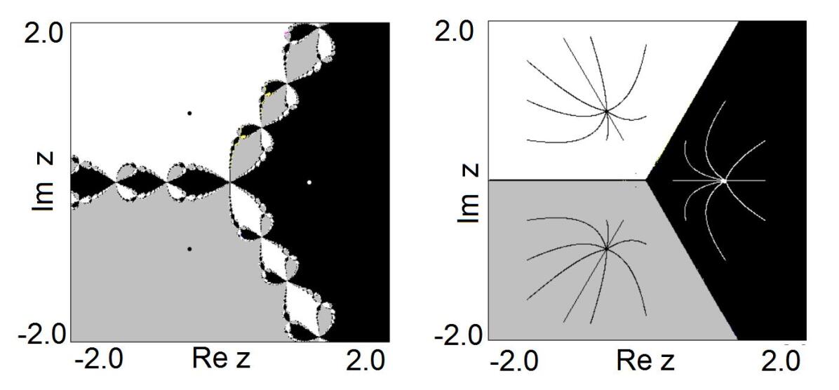
Figure 1: Newtonian Julia set — fractal boundary between white, black and gray regions, which are the basins of attraction of three roots of the equation (1) with $c=-1$ (left panel) and Newtonian pie — phase plane of the flow dynamical system (3) (right panel): three roots of (1) are the stable nodes of the ODE (3), its basins of attraction are divided by the smooth separatrix. Euler discretization (4) of (3) results in emergence of fractal basin boundary, like one on the left panel, which degenerates to the true smooth linear separatrix at $h\rightarrow 0$.

While in general discretization of flow dynamical systems caused by numerical time-integration can lead to emergence of solutions which do not represent the dynamics of the original system and manifest themselves in changes of the phase space structure, as in example discussed above, or changes in bifurcation diagrams etc. (see, e.g., [12, 16, 17] and references there), this problem can be considered from another angle: such discretization of well-known flow systems can be regarded as a fruitful approach, which is widely used in modern nonlinear theory and allows to generate new model maps (see, e.g., [2, 22, 11, 1] and references there). Due to emergence of numerical artifacts mentioned above dynamical systems generated this way can demonstrate various nontrivial phenomena. The discretization step $h$ is usually defined in such models in a wide range — moreover, it can be complex [18]. This approach can also establich a background for introducing and considering of a new class of systems, one example from which is proposed in present work.

Simple construction (2), being considered as an abstract dynamical system, allows a wide spectrum of generalizations and parametrizations. Types of dynamical behavior and obtained phenomena can also be rather diverse. Particularly, the implicit dynamics, when every point in the phase space of the system has both several images and several preimages [4, 3, 15], is also possible. Such implicit correspondences have wide spectrum of applications besides implicit numerical schemes of equations solving. Implicit functions can occur in problems of reconstruction of a multidimensional object (or system) from its projection [6], in the theory of generalized synchronization [19], in economics [10, 7], computer graphics [20], chaos control techniques [8], topology [21].

In the present paper we try to give an example of generalization of the iteration process (2) and to investigate obtained system from the point of view of theoretical nonlinear dynamics. In the section 1 we present the procedure of deriving an implicit map using the modified Euler method. In the section 2 we analyze the fractalization of both unstable and stable invariant sets of such exotic system.

1 Basic model

Among the numerical recipes of the ODE integration the semi-implicit Euler method is listed:

$$z_{n+1}=z_{n}+h(f(z_{n})+f(z_{n+1}))/2.$$ (6)

Let us generalize this scheme by parameterization:

$$z_{n+1}=z_{n}+h((1-\alpha)f(z_{n})+\alpha f(z_{n+1}).$$ (7)

In case when $f(z)$ chosen in form (5) this equation can be rewrited as following:

$$(\alpha h+3)z_{n+1}^{3}z_{n}^{2}+((1-\alpha)h-3)z_{n+1}^{2}z_{n}^{3}+(1-\alpha)hcz_{n+1}^{2}+\alpha hcz_{n}^{2}=0.$$ (8)

This is also some iteration process, but, in contrast to (4), not traditional for the nonlinear dynamical system theory. This is an implicit map with the evolution operator looking like

$$\Psi(z_{n+1},z_{n})=0.$$ (9)

Both forward and backward iterations of this map are defined by multi-valued functions,

$$z_{n+1}=\Psi_{+}(z_{n})$$ (10)

and

$$z_{n}=\Psi_{-}(z_{n+1})$$ (11)

respectively.

Two examples of implicit maps are described in [4, 9]. Below we are trying to study the implicit dynamics on the new example of such map (8).

2 Numerical simulation

2.1 Repellers

We will start investigation from studying backward dynamics of the map (8) at $\alpha=0$. In this case the map is single-valued time-forward and multi-valued time-backward. We will study structure of its repellers, which form boundaries of basins of attraction. It is worth mentioning here that since the map (8) is defined by the cubic polynomial, solutions of the equation (11) can be found analytically. The repellers of the map (8) at different values of $|h|\leq 1$ are shown in the Fig. 2. At $h=1$ we obtain the classical Newtonian Julia set, other positive values of $h$ correspond to transformations of this fractal (see Fig. 2a,b). Repellers in this case still define boundaries of areas of convergence of the Newton method (2) to different roots of (1) — or of the Euler method to different nodes of the ODE (3). At negative values of $h$ the process of search of repellers of the map (8) corresponds to solving the ODE (3) with the time reversed with the Euler method. The result of this process is a fractal set similar to the Sierpińsky gasket (see Fig. 2d,e). $h=0$ is a degenerate case corresponding transition between these two situations (see Fig. 2c,f).

The repellers for $h>1$ are shown in the Fig. 3, here $h=3$ (Fig. 3a) is also a degenerate case — which follows from the structure of function (8), where one of the terms becomes in this case equal to 0.

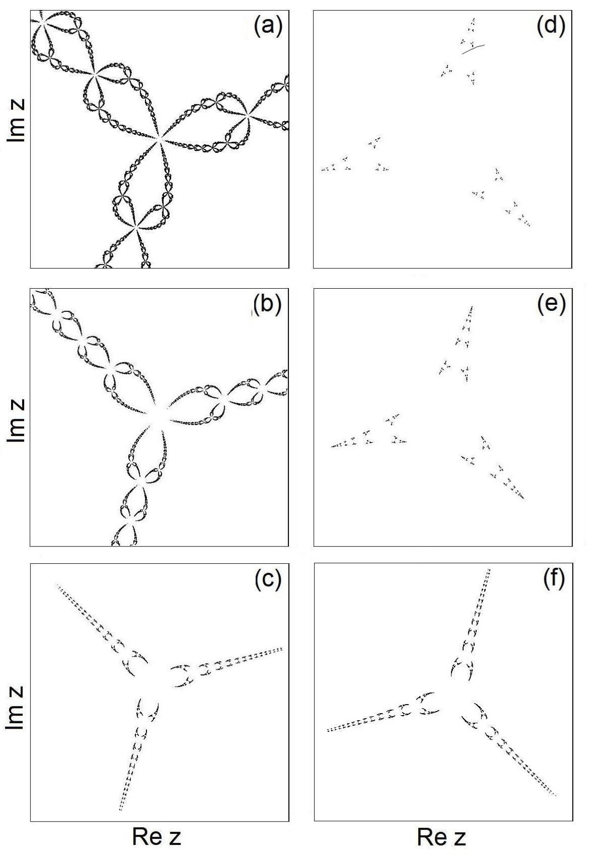
Figure 2: The repellers in the phase space of the map (8) with $h=1.0$ (a), $h=0.5$ (b), $h\rightarrow+0$ (c) and $h=-1.0$ (d), $h=-0.5$ (e), $h\rightarrow-0$ (f). Parameter $\alpha$ is equal to zero. Parameter $c$ is not essential, here and further it is fixed being equal to $(1-i)/2$.

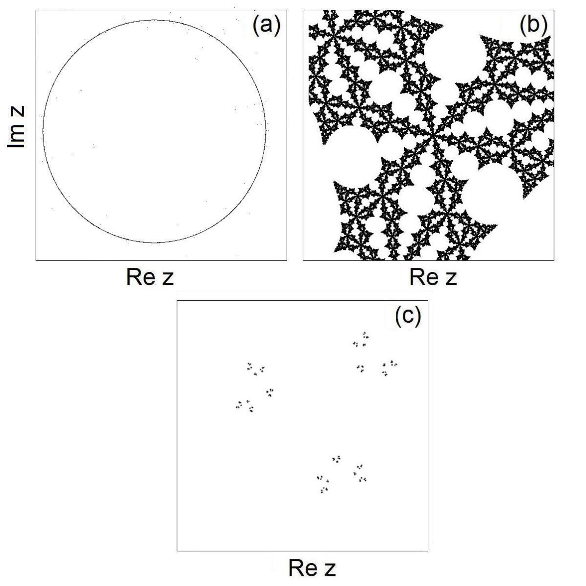
Figure 3: The repellers in the phase space of the map (8) with $\alpha=0$ and different values of $h$: $3$ (a), $5$ (b), $7$ (c).

A useful tool for quantitative analysis of the phase space structure transformations is a fractal dimension of the basin boundaries. Fig. 4 demonstrates the dependence of the box-counting dimension on the parameter $h$ value. In the vicinity of $h=0$ an abrupt change of the value of dimension occurs, which indicates a phase transition of the Julia set. In the vicinity of the degenerate case $h=3$ the fractal dimension value tends to 1 — it corresponds to degeneration of the Julia set, which looks in this case like a smooth circle (Fig. 3a). In the region near $h=4$ the value of dimension grows almost up to $2$, and Julia set almost becomes a fat fractal (Fig. 3b). When $h\geq 7$, the value of dimension decreases down to values below 1. The attracting invariant set undergoes here crisis, and basin boundaries degenerate to the fractal dust.

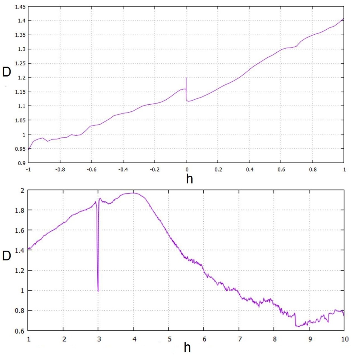
Figure 4: Box-counting dimension of the repellers of the implicit map (8) with $\alpha=0.0$ for $|h|\leq 1$ (upper panel) and $1\leq h\leq 10$ (bottom panel).

2.2 Attractors

In general case every point in the phase space of the implicit map (8) has three images — roots of qubic polynomial equation. Time-forward dynamics of such map is, as backward dynamics also, not single-valued. To study time-forward dynamics it seems productive to apply methods which are usually employed for an analysis of repellers. Particularly, we apply the “chaos game” algorithm [18] in order to find attracting chaotic trajectories. To find periodic trajectories we choose the roots of (8) at each iteration according to a periodic sequence. We construct symbolic codes, consisting of characters <<1>>, <<2>> and <<3>> — which correspond to the choice of the first, the second or the third root respectively. The period of dynamical orbit should be in this case equal or larger than a minimal period of such a sequence.

Let us start from the illustration of the evolution of attractors in special case $\alpha=0$, which is shown in the Fig. 5. This situation corresponds to the use of the explicit Euler method, and the forward-time dynamics is in this case single-valued. Fig. 5a represents three attracting nodes at $h\rightarrow 0$, while an increase of parameter $h$ causes several period doubling bifurcations (Fig. 5c-e), and the transition to chaos occurs (Fig. 5f).

The bifurcation diagram shown in the Fig. 6 gives more complete picture of the forward-time behavior of the system (8). Here the real part of the complex variable $z$ on the attracting invariant set is plotted versus parameter $h$. At this picture the evolution of one of three attracting fixed points is demonstrated. It undergoes several period-doubling bifurcations, transition to chaos and back to the periodic regime, and finally is destroyed via crisis. In the vicinity of the point $h=4$, where, as we mentioned above, Julia set almost becomes a fat fractal, time-forward dynamics is chaotic.

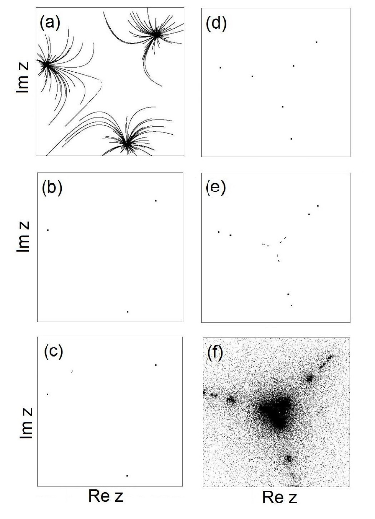
Figure 5: Transformation of the attracting invariant sets of the implicit map (8) with $\alpha=0.0$ and with $h\rightarrow 0$ (a), $h=0.5$ (b), 1.0 (c), 2.15 (d), 2.75 (e), 2.792 (f).

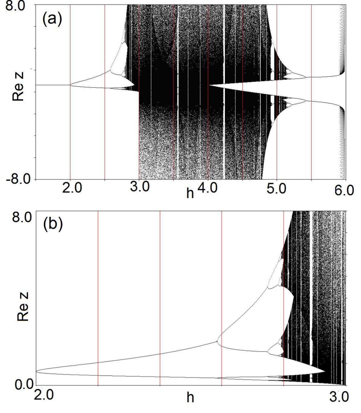
Figure 6: The bifurcation diagram for one of attracting invariant sets of the implicit map (8) with $\alpha=0.0$ (a) and its enlarged fragment (b).

Next Figure 7 demonstrates the picture of dynamical regimes on the parameter plane $(h,\alpha)$. When $\alpha\neq 0$, the map (8) becomes an implicit one, which means that its dynamics is now muti-valued both time-forward and time-backward.

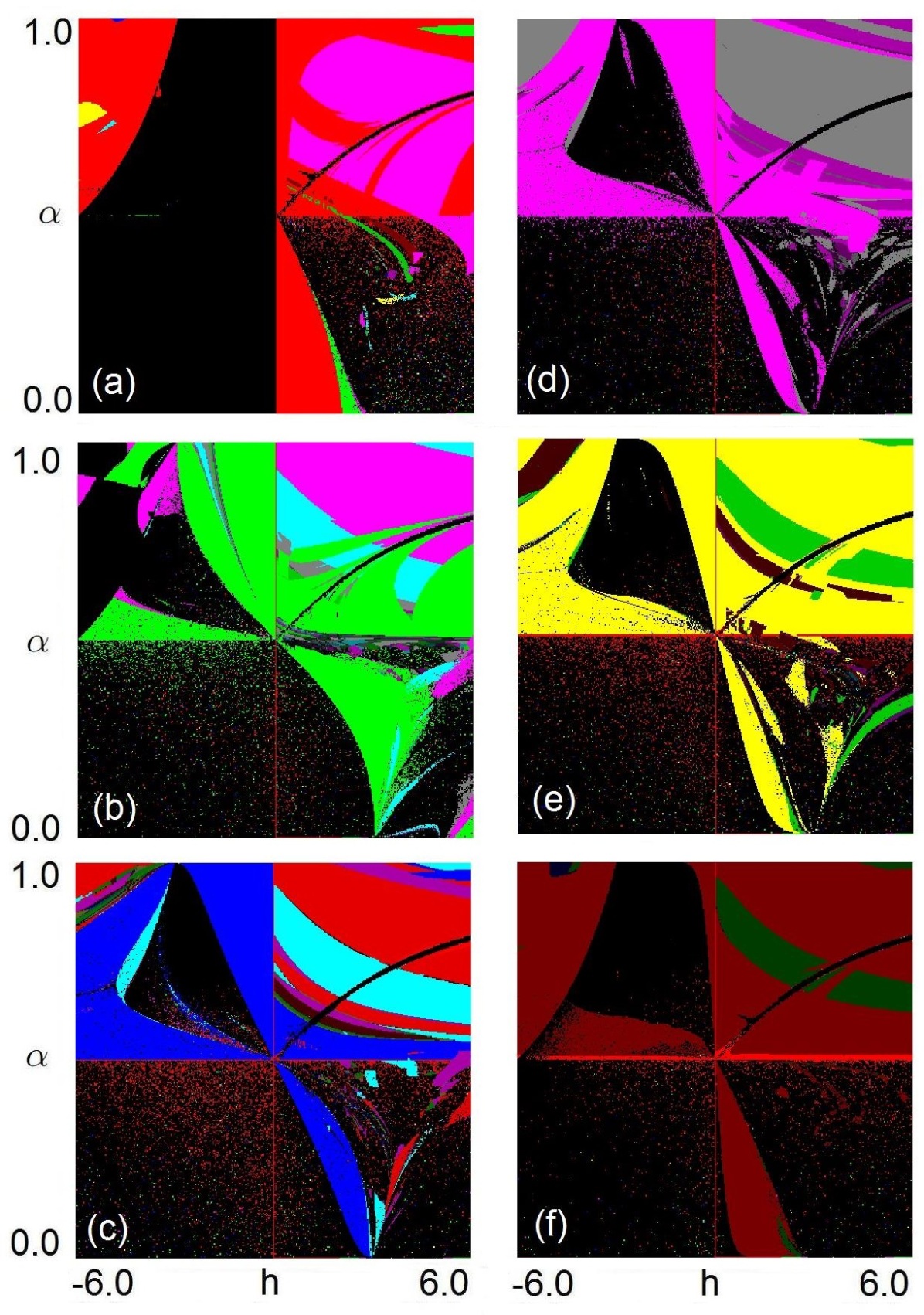
Figure 7: The charts of dynamical regimes of the implicit map (8) for the following periodic sequences of time-forward roots choice: $1$ (a), $12$ (b), $112$ (c), $1112~{}$(d), $11112$ (e), $1(\times 8)2$ (f).

Except the simplest case, when the symbolic sequence has period 1 (Fig. 7a), charts for different periodic sequences demonstrate similar features. Areas of periodic dynamics in the quadrant $(h>0,\alpha<0.5)$ have typical “tongue” shape with spikes in the point $\alpha=0,h=3$, where the map (8) is degenerate. Another typical feature is partial symmetry of the parameter plane: borders of areas of aperiodic dynamics are in many cases symmetrical with respect to the point $(h=0,\alpha=0.5)$ in quadrants $(h>0,\alpha<0.5)$ and $(h<0,\alpha>0.5)$, and points with periodic dynamics are symmetrical to points with aperiodic dynamic, especially for $|h|\leq 3$. It is a consequence of specific symmetry of the map (8), which is invariant with respect to the transformation $h\rightarrow-h,\alpha\rightarrow 1-\alpha,z_{n}\leftrightarrow z_{n+1}$.

3 Conclusion

In this paper we present a short preliminary view on the dynamics of one example of implicit systems, namely, the map (8). We demonstrate some approaches for studying of such systems. Advanced investigation of this implicit map should clarify the structure of its invariant sets. It seems a promising and very interesting direction of research, since in implicit systems, in contrast to traditionally studied explicit ones, an infinite number of trajectories can coexist in forward time, which makes their attracting invariant sets very complicated. Moreover, complexification of the parameter $h$ in the map (8) leads to the possibility of a situation, when $\Psi(z_{n+1},z_{n})=-\Psi^{*}(z_{n},z_{n+1})$. For the map (8) this happens at $h=\pm i$, $\alpha=1/2$. This situation, defined in [4, 9] as generalized unitarity, manifests the emergence of phenomena typical for Hamiltonian and almost Hamiltonian systems. In this context the implicit maps, being an artificial construct, can help to describe strong multistability, mixed dynamics and other complex phenomena of nonlinear dynamics.

References

- [1] Adilova, A.B., Kuznetsov, A.P., Savin, A.V.: Complex dynamics in the system of two coupled discrete R’́ossler oscillators. Izvestiya VUZ. Applied Nonlinear Dynamics 21(5), 108–119 (2013), (In Russian)
- [2] Arrowsmith, D.K., Cartwright, J.H., Lansbury, A.N., Place, C.M.: The Bogdanov map: Bifurcations, mode locking, and chaos in a dissipative system. International Journal of Bifurcation and Chaos 3(04), 803–842 (1993)
- [3] Bullett, S.R.: Dynamics of quadratic correspondences. Nonlinearity 1(1), 27–50 (1988)
- [4] Bullett, S.R., Osbaldestin, A.H., Percival, I.C.: An iterated implicit complex map. Physica D: Nonlinear Phenomena 19(2), 290–300 (1986)
- [5] Cayley, A.: Desiderata and suggestions: no. 3. The Newton-Fourier imaginary problem. American Journal of Mathematics 2(1), 97–97 (1879)
- [6] DiFranco, D.E., Cham, T.J., Rehg, J.M.: Reconstruction of 3D figure motion from 2D correspondences. In: Proceedings of the 2001 IEEE Computer Society Conference on Computer Vision and Pattern Recognition. CVPR 2001. vol. 1, pp. 307–314. IEEE (2001)
- [7] Gardini, L., Hommes, C., Tramontana, F., De Vilder, R.: Forward and backward dynamics in implicitly defined overlapping generations models. Journal of Economic Behavior & Organization 71(2), 110–129 (2009)
- [8] Hill, D.: Control of implicit chaotic maps using nonlinear approximations. Chaos: An Interdisciplinary Journal of Nonlinear Science 10(3), 676–681 (2000)
- [9] Isaeva, O.B., Obychev, M.A., Savin, D.V.: Dynamics of a discrete system with the operator of evolution given by an implicit function: from the Mandelbrot map to a unitary map. Russian Journal of Nonlinear Dynamics 13(3), 331–348 (2017), (In Russian)
- [10] Kennedy, J.A., Stockman, D.R.: Chaotic equilibria in models with backward dynamics. Journal of Economic Dynamics and Control 32(3), 939–955 (2008)
- [11] Kuznetsov, A.P., Savin, A.V., Sedova, Y.V.: Bogdanov-Takens bifurcation: from flows to discrete systems. Izvestiya VUZ. Applied Nonlinear Dynamics 17(6), 139–158 (2009), (In Russian)
- [12] Lóczi, L., Páez Chávez, J.: Preservation of bifurcations under Runge-Kutta methods. International Journal of Qualitative Theory of Differential Equations and Applications 3, 81–98 (2008)
- [13] Magreñán, Á.A., Gutiérrez, J.M.: Real dynamics for damped Newton’s method applied to cubic polynomials. Journal of Computational and Applied Mathematics 275, 527–538 (2015)
- [14] McLaughlin, J.: Convergence of a relaxed Newton’s method for cubic equations. Computers & chemical engineering 17(10), 971–983 (1993)
- [15] Mestel, B.D., Osbaldestin, A.H.: Renormalisation in implicit complex maps. Physica D: Nonlinear Phenomena 39(2-3), 149–162 (1989)
- [16] Páez Chávez, J.: Discretizing bifurcation diagrams near codimension two singularities. International Journal of Bifurcation and Chaos 20(5), 1391–1403 (2010)
- [17] Páez Chávez, J.: Discretizing dynamical systems with generalized Hopf bifurcations. Numerische Mathematik 118(2), 229–246 (2011)
- [18] Peitgen, H.O., Richter, P.H.: The beauty of fractals: images of complex dynamical systems. Springer Science & Business Media (1986)
- [19] Pikovsky, A., Rosenblum, M., Kurths, J.: Synchronization: A Universal Concept in Nonlinear Sciences. Cambridge Nonlinear Science Series, Cambridge University Press (2001)
- [20] Sclaroff, S., Pentland, A.: Generalized implicit functions for computer graphics. ACM Siggraph Computer Graphics 25(4), 247–250 (1991)
- [21] Vlasenko, I.Y.: Internal maps: topological invariants and their applications. Proceedings of Institute of Mathematics of Ukrainian NAS, Institute of Mathematics of Ukrainian NAS (2014), (In Russian)
- [22] Zaslavsky, G.M.: The physics of chaos in Hamiltonian systems. World Scientific (2007)