Modelling frequency-dependent tidal deformability
for environmental black-hole mergers
Abstract
Motivated by events in which black holes can lose their environment due to tidal interactions in a binary system, we develop a waveform model in which the tidal deformability interpolates between a finite value (dressed black hole) at relatively low frequency and a zero value (naked black hole) at high frequency. We then apply this model to the example case of a black hole dressed with an ultralight scalar field and investigate the detectability of the tidal Love number with the Einstein Telescope. We show that the parameters of the tidal deformability model could be measured with high accuracy, providing a useful tool to understand dynamical environmental effects taking place during the inspiral of a binary system.
I Introduction
Tidal interactions in close astrophysical systems carry golden information on the internal composition of compact objects. They affect the dynamics of binary sources, leaving a footprint within the emitted signals, both in the gravitational-wave (GW) and in the electromagnetic spectrum Poisson and Will (2014). Pioneering calculations, performed at the beginning of the twentieth century, have paved the ground for a rigorous analytical description of tidal effects in terms of a set of quantities, the tidal Love numbers (TLNs), which encode the deformability properties of self-gravitating bodies Love (1909). Initially exploited to study the structure of planets in the Solar System within Newtonian gravity, TLNs have been generalised to a fully relativistic description Hinderer (2008); Binnington and Poisson (2009); Damour and Nagar (2009), and have raised considerable attention in the context of binary neutron star (NS) mergers, with the tantalising possibility of constraining the equation of state of dense matter from GW observations Baiotti et al. (2010, 2011); Vines et al. (2011); Pannarale et al. (2011); Vines and Flanagan (2013); Lackey et al. (2012, 2014); Flanagan and Hinderer (2008); Favata (2014); Yagi and Yunes (2014); Maselli et al. (2013a, b); Del Pozzo et al. (2013); Abbott et al. (2017a); Bauswein et al. (2017); Most et al. (2018); Harry and Hinderer (2018); Annala et al. (2018); Abbott et al. (2018); Akcay et al. (2019); Abdelsalhin et al. (2018); Jiménez Forteza et al. (2018); Banihashemi and Vines (2020); Dietrich et al. (2019, 2021); Henry et al. (2020); Pacilio et al. (2022); Maselli et al. (2021) (see Refs. Guerra Chaves and Hinderer (2019); Chatziioannou (2020) for some reviews).
More recently, measurements of the TLNs from compact binaries have been proposed as a new tool to infer the properties of the environment in which the systems evolve. This possibility arises from the remarkable result that, within General Relativity, the TLNs of naked black holes (BHs) (i.e., BHs in vacuum) vanish Binnington and Poisson (2009); Damour and Nagar (2009); Damour and Lecian (2009); Pani et al. (2015a, b); Gürlebeck (2015); Porto (2016); Le Tiec and Casals (2021); Chia (2021); Le Tiec et al. (2021). This property however is fragile, as it is broken for BH mimickers Cardoso et al. (2017), in extended theories of gravity Cardoso et al. (2017, 2018); De Luca et al. (2022), in higher dimensions Kol and Smolkin (2012); Cardoso et al. (2019); Hui et al. (2021), or in nonvacuum environments Baumann et al. (2019); Cardoso and Duque (2020); De Luca and Pani (2021); Cardoso et al. (2022). In particular, during their cosmological evolution, environmental effects may provide an effective dress to BHs, resulting in nonzero TLNs. Such dresses may be formed around BHs due to secular effects like accretion111Accretion-driven dresses may be particularly important for primordial BHs, which are expected to be surrounded by a dark matter halo if they do not comprise the totality of the dark matter in the universe Mack et al. (2007); Adamek et al. (2019). The detection of tidal effects can thus be used to distinguish primordial BHs (with their clouds) from other scenarios Franciolini et al. (2022). or superradiant instabilities of ultralight bosonic fields Brito et al. (2015), for which it has been shown that the TLNs would be proportional to inverse powers of the boson mass Baumann et al. (2019); De Luca and Pani (2021).
Love numbers of dressed BHs could be sufficiently large to leave an observable signature within GW signals emitted by coalescing binaries and, if measured, they could provide a smoking gun for the existence of nonvacuum “structures” close to BHs. Unlike NS matter however, a low-density environmental dress may be unravelled during the last phases of the inspiral. In analogy with mass-shedding events occurring for stars with small compactness, disruption of the dress usually takes place when the binary semi-major axis is comparable with the Roche radius Shapiro and Teukolsky (1983). For smaller orbital radii, the environment progressively disappears and the coalescence proceeds with two naked BHs. This process can be modelled through time-dependent TLNs, that smoothly approach zero.222Note that this is different from the notion of dynamical tidal deformability investigated in Steinhoff et al. (2016); Creci et al. (2021); Consoli et al. (2022) (see also Nair et al. (2022)). In our case the TLNs are time-dependent because of the gradual disappearance of the environment around a BH, while the dynamical tidal deformability defined in Steinhoff et al. (2016); Creci et al. (2021); Consoli et al. (2022) measures the BH response to time-dependent tidal perturbations. A similar phenomenon may occur when, during the common envelope phase of a neutron star binary, at least one of the objects with a mass very close to the Chandrasekhar limit turns into a BH Singh et al. (2022), changing its TLNs from a finite value to zero.
The scope of this work is to study the relevance of such effect on BH binaries potentially observable by third-generation (3G) detectors like the Einstein Telescope (ET) or Cosmic Explorer Dwyer et al. (2015); Hild et al. (2011); Sathyaprakash et al. (2019); Maggiore et al. (2020); Essick et al. (2017); Abbott et al. (2017b), and to assess their ability to constrain the features of time-varying TLNs. We embed the latter within a BH waveform template properly built to model a smooth transition of the TLNs to zero, showing how few GW observations could shed new light on the matter content of the binary environment, and on the dynamical processes that lead to its tidal disruption. Hereafter we use geometric units, .
II Setup
We model the GW signal emitted by the binary using a modified version of the IMRPhenomD waveform model, which takes into account the inspiral, merger and ringdown phases of the coalescence Husa et al. (2016); Khan et al. (2016). The inspiral regime is further broken-up into an early and a late component, with the former being described by the post-Newtonian (PN) expansion, in which tidal effects add linearly to point-particle contributions and are fully encoded by the Love numbers. In Fourier space, the early part of the signal is given by Sathyaprakash and Dhurandhar (1991); Damour et al. (2000),
| (1) |
where contains terms up to the 3.5PN order Damour et al. (2000); Arun et al. (2005); Buonanno et al. (2009); Abdelsalhin et al. (2018), and depends on the binary chirp mass and the symmetric mass ratio , where are the component masses. The phase also includes linear spin terms up to 3PN order through the (anti)symmetric combinations of the individual spin components and , and quadratic spin corrections entering at 2PN order, which include the spin-induced quadrupole moments. For sake of simplicity we assume that the latter correspond to their (naked) Kerr values, and that the effect of the dress is subdominant. An additional contribution to the GW phase comes from tidal heating, which depends on the energy absorbed at the horizon and is proportional to the BH cross section. This effect introduces a higher-order PN correction Alvi (2001); Maselli et al. (2018), which is typically small and negligible for our analysis, and hence we assume that is the same as for naked BHs De Luca and Pani (2021). The waveform amplitude , also expanded up to the 3PN order, depends on , with the leading term reading
| (2) |
where is the luminosity distance. Finally the geometric factor depends on the inclination which identifies the angle between the binary line of sight and its orbital angular momentum, and on the detector antenna pattern functions which are functions of the source position in the sky and on the polarization angle .
The dominant tidal correction enters the waveform at the 5PN order as , in terms of the total mass of the binary and of the effective tidal deformability parameter , which depends on the masses and TLNs of each binary component Flanagan and Hinderer (2008); Vines et al. (2011). We neglect higher-order PN contributions (starting at 6PN order) since they are hardly measurable and increase the dimensionality of the parameter space.
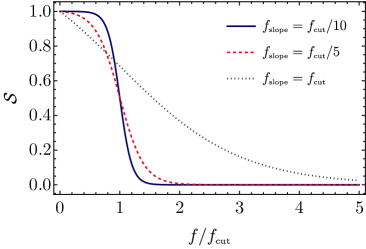
We assume that the halo surroundings the BHs is dynamically disrupted during the coalescence, i.e. that tidal effects disappear progressively from a characteristic cut-off frequency . To this aim we introduce a frequency-dependent tidal deformability
| (3) |
which is cast in terms of a smoothing function that approaches zero at frequencies larger than the cut-off with a characteristic slope . A representative example of the smoothing function is shown in Fig. 1. In our analysis tidal effects are therefore fully described by three quantities, , while the overall waveform model depends on 14 parameters , where are the time and phase at the coalescence.
We study the detectability of the tidal parameters by using a Fisher-matrix approach Poisson and Will (1995); Vallisneri (2008); Cardoso et al. (2017). For signals with large signal-to-noise ratio (snr), as those expected for 3G detectors, the posterior distribution of can be described by a multivariate Gaussian distribution centered around the true values , with covariance , where
| (4) |
is the Fisher information matrix, and statistical error on the -th parameter is given by . In the previous expression we have introduced the scalar product over the detector noise spectral density between two waveform templates :
| (5) |
where denotes complex conjugation. The snr of a given signal is . In our analysis we fix the minimum and maximum frequency of integration to Hz and , where is the remnant’s ringdown frequency Khan et al. (2016).
Hereafter we consider optimally-oriented binaries, removing the four angles from the Fisher analysis, thus reducing to a square matrix. We also fix and . We assume that dressed binary BHs are observed by ET adopting the design ET-D sensitivity curve Hild et al. (2011).
III Results
III.1 General framework
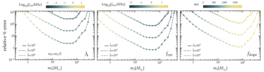
We apply the framework discussed above to investigate the detectability of the tidal parameters. The results of the Fisher analysis are shown in Fig. 2, for different choices of . Larger values would break the convergence of the post-Newtonian expansion, leading the tidal term to dominate over the lower PN orders. For simplicity we focus on binaries with mass ratio , although both masses are included as waveform parameters of the Fisher analysis. Different choices provide similar results. The ISCO frequency for each binary is computed taking into account self-force effects due to the lighter component of the binary Favata (2011).
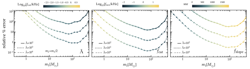
The top panels of Fig. 2 assume and for the cut-off and slope frequency, respectively. Note that for all binary configurations analysed we have checked that the cut-off frequency is (well) below the frequency describing the transition between the early and the late inspiral, Husa et al. (2016); Khan et al. (2016). The panels of Fig. 2 show that all the tidal parameters can be measured with high accuracy for sufficiently large values of the effective tidal Love number. In particular, considering a dressed BH system with primary mass and mass ratio at a distance , ET will be able to measure its tidal deformability with a relative accuracy of a few percent and an snr of a few hundred. A similar precision can be reached for the cut-off and the slope frequency of the smoothing function, showing the potential of ET in measuring the transition point where the TLN vanishes. These results slightly improve if we assume and , as shown in the bottom panels of Fig. 2. This is expected since larger value of the cut-off frequency translates into a longer inspiral phase in which tidal effects are active. Changing the slope frequency does not significantly modify the results of our analysis. For example, we have checked that a decrease in , which results into a sharper cut-off, does not strongly impact on the estimated errors.
III.2 First-principle model: BHs dressed by ultralight bosons
We can now focus on a specific example of a dress sourced by an ultralight bosonic scalar field with mass undertaking a phase of accretion or superradiant instability Brito et al. (2015) onto a BH. In this case it was shown that the TLN of each body is proportional to the inverse of the gravitational coupling , namely De Luca and Pani (2021)
| (6) |
where . For this model, the effective tidal deformability vanishes when the clouds surrounding each binary component are tidally disrupted, that is when the binary semi-major axis is comparable to the Roche radius. For different binary components this results into different cut-off frequencies for each body. We therefore introduce an effective frequency-dependent TLN as , where each smoothing function is determined by the same slope frequency , but by different cut-off frequencies De Luca and Pani (2021)
| (7) |
in terms of a numerical coefficient which takes values from 1.26 for rigid bodies to 2.44 for fluid ones, and of the total mass enclosed in the scalar cloud . We fix the latter to the upper bound , which saturates the regime of validity of the perturbative expansion. Note that, in a first-principle model such as this one, the number of waveform parameters to be constrained is smaller than in the general model, since the gravitational couplings dictate both the TLNs and the cut-off frequencies.
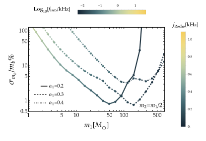
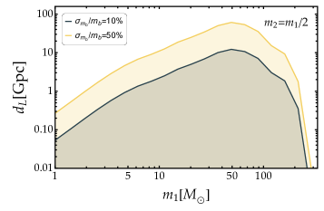
The results for the Fisher analysis for this case are shown in Fig. 3. The left panel shows the relative percentage error on the gravitational coupling as a function of the primary BH mass, assuming a luminosity distance of and mass ratio . The upper and lateral bars identify the corresponding ISCO and Roche frequencies, respectively. One can appreciate that in the mass range ET could measure the coupling with an accuracy of a few percent. This result improves the one discussed in De Luca and Pani (2021) where the integration in Eq. (5) was cut at the ISCO frequency, also assuming the signal amplitude to vanish afterward. Frequencies after the cut-off, which can be consistently taken into account within the PhenomD waveform model, provide here a significant boost to the parameter’s reconstruction, which in turn translates into an improvement on the errors of the tidal parameters.333Note that, within our general model, the results of De Luca and Pani (2021) can be recovered in the limit, where effectively the tidal part of the signal vanishes for . In the right panel of Fig. 3 we show the maximum luminosity distance for which ET would be able to constrain the scalar field mass with a relative percentage error of (green line) and (yellow line), assuming a gravitational coupling . The result shows that ET could measure the scalar field mass with high accuracy within distances of a few Gpc.
Finally, let us stress that, as tidal interactions take place and lead to the disruption of the clouds, the effective mass of the BH+halo system decreases, probably resulting into a naked binary system coalescing within an unbound and more diluted halo. As a proof of concept, in order to estimate the effect of this mass decrease in the waveforms, we have introduced a similar suppression factor as the one discussed above to the BH masses, i.e. , which interpolates between unity and , as the cloud’s mass accounts at most for about 10% of the BH masses in relevant scenario like superradiance. By introducing this frequency-dependent factor for the masses through all PN orders, we found that the error on increases by only a factor of 2, while the errors on and become much smaller, as these parameters appear also at lower PN orders and are therefore better constrained. Another interesting extension is to account for the orbital energy loss associated with the halo disruption Baumann et al. (2022a, b). We leave a better investigation of these interesting effects to future work.
IV Conclusions
Tidal interactions active during the inspiral phase of binary coalescences carry unique information on the internal structure of compact objects and on the properties of the surroundings in which the systems evolve. BHs dressed by a halo formed by dark matter, by a phase of accretion, or by the superradiant instability of a ultralight boson, provide some astrophysical scenarios in which the external environments leave a footprint on the emitted GW signal Cole et al. (2022), encoded in particular in nonvanishing TLNs Baumann et al. (2019); Cardoso and Duque (2020); De Luca and Pani (2021); Cardoso et al. (2022). In these cases, however, the gravitational interaction with the BH companion may destroy the halo, leading to tidal effects that fade away in the waveform at higher frequency.
Motivated by such examples, in this paper we have investigated the potential of 3G detectors like ET to measure the variation of the Love number once the binary inspiral crosses a given cut-off frequency. To this aim we have augmented the standard IMRphenomD waveform with the inclusion of an effective tidal deformability which interpolates the transition between a finite effective Love number and the full vacuum regime. We have carried out a statistical analysis on a wide range of sources observable by ET, finding that, together with , both the cut-off frequency and the slope of the effective deformability are potentially measurable, with an accuracy of a few percent for stellar mass binaries. The simultaneous measurements of all tidal parameters would provide key information on the composition of the BH environment, and on the mechanisms responsible for the vanishing of the Love number.
These results also pave the avenue for multiband analyses between ET and LISA Amaro-Seoane et al. (2017), for sources in a specific mass range Sesana (2016); Vitale (2016). For example, one can envisage a scenario in which a binary system of two dressed BHs with masses inspirals within the frequency band of LISA, with a cut-off frequency falling into the ET bandwidth. A statistical analysis for LISA only would suggest that all the parameters of the effective tidal deformability are unmeasurable. However, a joint analysis which takes into account that the binary keeps evolving in ET with fading Love number, would dramatically improve the parameter reconstruction. For a - binary, and assuming , the multiband analysis would lead to a stringent constraint on the environment Love number at the level of .
Finally, let us stress that a frequency-dependent TLN can be used to disentangle dressed BHs from neutron stars in the solar mass range, since the latter are characterised by tidal effects which persist until the last stages of the merger. We plan to investigate this point in a future work.
Acknowledgements.
We thank G. Franciolini for interesting comments. A.M. thanks the University of Pennsylvania for the hospitality during the completion of this project. V.DL. is supported by funds provided by the Center for Particle Cosmology at the University of Pennsylvania. A.M. acknowledges financial support from the EU Horizon 2020 Research and Innovation Programme under the Marie Sklodowska-Curie Grant Agreement no. 101007855. P.P. acknowledges support provided under the European Union’s H2020 ERC, Starting Grant agreement no. DarkGRA–757480 and under the MIUR PRIN programme, and support from the Amaldi Research Center funded by the MIUR program “Dipartimento di Eccellenza” (CUP: B81I18001170001).References
- Poisson and Will (2014) E. Poisson and C. M. Will, Gravity: Newtonian, Post-Newtonian, Relativistic (Cambridge University Press, 2014).
- Love (1909) A. E. H. Love, Mont. Not. Roy. Astr. Soc. 69, 476 (1909).
- Hinderer (2008) T. Hinderer, Astrophys. J. 677, 1216 (2008), arXiv:0711.2420 [astro-ph] .
- Binnington and Poisson (2009) T. Binnington and E. Poisson, Phys. Rev. D 80, 084018 (2009), arXiv:0906.1366 [gr-qc] .
- Damour and Nagar (2009) T. Damour and A. Nagar, Phys. Rev. D 80, 084035 (2009), arXiv:0906.0096 [gr-qc] .
- Baiotti et al. (2010) L. Baiotti, T. Damour, B. Giacomazzo, A. Nagar, and L. Rezzolla, Phys. Rev. Lett. 105, 261101 (2010), arXiv:1009.0521 [gr-qc] .
- Baiotti et al. (2011) L. Baiotti, T. Damour, B. Giacomazzo, A. Nagar, and L. Rezzolla, Phys. Rev. D 84, 024017 (2011), arXiv:1103.3874 [gr-qc] .
- Vines et al. (2011) J. Vines, E. E. Flanagan, and T. Hinderer, Phys. Rev. D 83, 084051 (2011), arXiv:1101.1673 [gr-qc] .
- Pannarale et al. (2011) F. Pannarale, L. Rezzolla, F. Ohme, and J. S. Read, Phys. Rev. D 84, 104017 (2011), arXiv:1103.3526 [astro-ph.HE] .
- Vines and Flanagan (2013) J. E. Vines and E. E. Flanagan, Phys. Rev. D 88, 024046 (2013), arXiv:1009.4919 [gr-qc] .
- Lackey et al. (2012) B. D. Lackey, K. Kyutoku, M. Shibata, P. R. Brady, and J. L. Friedman, Phys. Rev. D 85, 044061 (2012), arXiv:1109.3402 [astro-ph.HE] .
- Lackey et al. (2014) B. D. Lackey, K. Kyutoku, M. Shibata, P. R. Brady, and J. L. Friedman, Phys. Rev. D 89, 043009 (2014), arXiv:1303.6298 [gr-qc] .
- Flanagan and Hinderer (2008) E. E. Flanagan and T. Hinderer, Phys. Rev. D 77, 021502 (2008), arXiv:0709.1915 [astro-ph] .
- Favata (2014) M. Favata, Phys. Rev. Lett. 112, 101101 (2014), arXiv:1310.8288 [gr-qc] .
- Yagi and Yunes (2014) K. Yagi and N. Yunes, Phys. Rev. D 89, 021303 (2014), arXiv:1310.8358 [gr-qc] .
- Maselli et al. (2013a) A. Maselli, V. Cardoso, V. Ferrari, L. Gualtieri, and P. Pani, Phys. Rev. D 88, 023007 (2013a), arXiv:1304.2052 [gr-qc] .
- Maselli et al. (2013b) A. Maselli, L. Gualtieri, and V. Ferrari, Phys. Rev. D 88, 104040 (2013b), arXiv:1310.5381 [gr-qc] .
- Del Pozzo et al. (2013) W. Del Pozzo, T. G. F. Li, M. Agathos, C. Van Den Broeck, and S. Vitale, Phys. Rev. Lett. 111, 071101 (2013), arXiv:1307.8338 [gr-qc] .
- Abbott et al. (2017a) B. P. Abbott et al. (LIGO Scientific, Virgo), Phys. Rev. Lett. 119, 161101 (2017a), arXiv:1710.05832 [gr-qc] .
- Bauswein et al. (2017) A. Bauswein, O. Just, H.-T. Janka, and N. Stergioulas, Astrophys. J. Lett. 850, L34 (2017), arXiv:1710.06843 [astro-ph.HE] .
- Most et al. (2018) E. R. Most, L. R. Weih, L. Rezzolla, and J. Schaffner-Bielich, Phys. Rev. Lett. 120, 261103 (2018), arXiv:1803.00549 [gr-qc] .
- Harry and Hinderer (2018) I. Harry and T. Hinderer, Class. Quant. Grav. 35, 145010 (2018), arXiv:1801.09972 [gr-qc] .
- Annala et al. (2018) E. Annala, T. Gorda, A. Kurkela, and A. Vuorinen, Phys. Rev. Lett. 120, 172703 (2018), arXiv:1711.02644 [astro-ph.HE] .
- Abbott et al. (2018) B. P. Abbott et al. (LIGO Scientific, Virgo), Phys. Rev. Lett. 121, 161101 (2018), arXiv:1805.11581 [gr-qc] .
- Akcay et al. (2019) S. Akcay, S. Bernuzzi, F. Messina, A. Nagar, N. Ortiz, and P. Rettegno, Phys. Rev. D 99, 044051 (2019), arXiv:1812.02744 [gr-qc] .
- Abdelsalhin et al. (2018) T. Abdelsalhin, L. Gualtieri, and P. Pani, Phys. Rev. D 98, 104046 (2018), arXiv:1805.01487 [gr-qc] .
- Jiménez Forteza et al. (2018) X. Jiménez Forteza, T. Abdelsalhin, P. Pani, and L. Gualtieri, Phys. Rev. D 98, 124014 (2018), arXiv:1807.08016 [gr-qc] .
- Banihashemi and Vines (2020) B. Banihashemi and J. Vines, Phys. Rev. D 101, 064003 (2020), arXiv:1805.07266 [gr-qc] .
- Dietrich et al. (2019) T. Dietrich, A. Samajdar, S. Khan, N. K. Johnson-McDaniel, R. Dudi, and W. Tichy, Phys. Rev. D 100, 044003 (2019), arXiv:1905.06011 [gr-qc] .
- Dietrich et al. (2021) T. Dietrich, T. Hinderer, and A. Samajdar, Gen. Rel. Grav. 53, 27 (2021), arXiv:2004.02527 [gr-qc] .
- Henry et al. (2020) Q. Henry, G. Faye, and L. Blanchet, Phys. Rev. D 102, 044033 (2020), arXiv:2005.13367 [gr-qc] .
- Pacilio et al. (2022) C. Pacilio, A. Maselli, M. Fasano, and P. Pani, Phys. Rev. Lett. 128, 101101 (2022), arXiv:2104.10035 [gr-qc] .
- Maselli et al. (2021) A. Maselli, A. Sabatucci, and O. Benhar, Phys. Rev. C 103, 065804 (2021), arXiv:2010.03581 [astro-ph.HE] .
- Guerra Chaves and Hinderer (2019) A. Guerra Chaves and T. Hinderer, J. Phys. G 46, 123002 (2019), arXiv:1912.01461 [nucl-th] .
- Chatziioannou (2020) K. Chatziioannou, Gen. Rel. Grav. 52, 109 (2020), arXiv:2006.03168 [gr-qc] .
- Damour and Lecian (2009) T. Damour and O. M. Lecian, Phys. Rev. D 80, 044017 (2009), arXiv:0906.3003 [gr-qc] .
- Pani et al. (2015a) P. Pani, L. Gualtieri, A. Maselli, and V. Ferrari, Phys. Rev. D 92, 024010 (2015a), arXiv:1503.07365 [gr-qc] .
- Pani et al. (2015b) P. Pani, L. Gualtieri, and V. Ferrari, Phys. Rev. D 92, 124003 (2015b), arXiv:1509.02171 [gr-qc] .
- Gürlebeck (2015) N. Gürlebeck, Phys. Rev. Lett. 114, 151102 (2015), arXiv:1503.03240 [gr-qc] .
- Porto (2016) R. A. Porto, Fortsch. Phys. 64, 723 (2016), arXiv:1606.08895 [gr-qc] .
- Le Tiec and Casals (2021) A. Le Tiec and M. Casals, Phys. Rev. Lett. 126, 131102 (2021), arXiv:2007.00214 [gr-qc] .
- Chia (2021) H. S. Chia, Phys. Rev. D 104, 024013 (2021), arXiv:2010.07300 [gr-qc] .
- Le Tiec et al. (2021) A. Le Tiec, M. Casals, and E. Franzin, Phys. Rev. D 103, 084021 (2021), arXiv:2010.15795 [gr-qc] .
- Cardoso et al. (2017) V. Cardoso, E. Franzin, A. Maselli, P. Pani, and G. Raposo, Phys. Rev. D 95, 084014 (2017), [Addendum: Phys.Rev.D 95, 089901 (2017)], arXiv:1701.01116 [gr-qc] .
- Cardoso et al. (2018) V. Cardoso, M. Kimura, A. Maselli, and L. Senatore, Phys. Rev. Lett. 121, 251105 (2018), arXiv:1808.08962 [gr-qc] .
- De Luca et al. (2022) V. De Luca, J. Khoury, and S. S. C. Wong, (2022), arXiv:2211.14325 [hep-th] .
- Kol and Smolkin (2012) B. Kol and M. Smolkin, JHEP 02, 010 (2012), arXiv:1110.3764 [hep-th] .
- Cardoso et al. (2019) V. Cardoso, L. Gualtieri, and C. J. Moore, Phys. Rev. D 100, 124037 (2019), arXiv:1910.09557 [gr-qc] .
- Hui et al. (2021) L. Hui, A. Joyce, R. Penco, L. Santoni, and A. R. Solomon, JCAP 04, 052 (2021), arXiv:2010.00593 [hep-th] .
- Baumann et al. (2019) D. Baumann, H. S. Chia, and R. A. Porto, Phys. Rev. D 99, 044001 (2019), arXiv:1804.03208 [gr-qc] .
- Cardoso and Duque (2020) V. Cardoso and F. Duque, Phys. Rev. D 101, 064028 (2020), arXiv:1912.07616 [gr-qc] .
- De Luca and Pani (2021) V. De Luca and P. Pani, JCAP 08, 032 (2021), arXiv:2106.14428 [gr-qc] .
- Cardoso et al. (2022) V. Cardoso, K. Destounis, F. Duque, R. P. Macedo, and A. Maselli, Phys. Rev. D 105, L061501 (2022), arXiv:2109.00005 [gr-qc] .
- Mack et al. (2007) K. J. Mack, J. P. Ostriker, and M. Ricotti, Astrophys. J. 665, 1277 (2007), arXiv:astro-ph/0608642 .
- Adamek et al. (2019) J. Adamek, C. T. Byrnes, M. Gosenca, and S. Hotchkiss, Phys. Rev. D 100, 023506 (2019), arXiv:1901.08528 [astro-ph.CO] .
- Franciolini et al. (2022) G. Franciolini, R. Cotesta, N. Loutrel, E. Berti, P. Pani, and A. Riotto, Phys. Rev. D 105, 063510 (2022), arXiv:2112.10660 [astro-ph.CO] .
- Brito et al. (2015) R. Brito, V. Cardoso, and P. Pani, Lect. Notes Phys. 906, pp.1 (2015), arXiv:1501.06570 [gr-qc] .
- Shapiro and Teukolsky (1983) S. L. Shapiro and S. A. Teukolsky, Black holes, white dwarfs, and neutron stars: The physics of compact objects (1983).
- Steinhoff et al. (2016) J. Steinhoff, T. Hinderer, A. Buonanno, and A. Taracchini, Phys. Rev. D 94, 104028 (2016), arXiv:1608.01907 [gr-qc] .
- Creci et al. (2021) G. Creci, T. Hinderer, and J. Steinhoff, Phys. Rev. D 104, 124061 (2021), [Erratum: Phys.Rev.D 105, 109902 (2022)], arXiv:2108.03385 [gr-qc] .
- Consoli et al. (2022) D. Consoli, F. Fucito, J. F. Morales, and R. Poghossian, (2022), arXiv:2206.09437 [hep-th] .
- Nair et al. (2022) S. Nair, S. Chakraborty, and S. Sarkar, (2022), arXiv:2208.06235 [gr-qc] .
- Singh et al. (2022) D. Singh, A. Gupta, E. Berti, S. Reddy, and B. S. Sathyaprakash, (2022), arXiv:2210.15739 [gr-qc] .
- Dwyer et al. (2015) S. Dwyer, D. Sigg, S. W. Ballmer, L. Barsotti, N. Mavalvala, and M. Evans, Phys. Rev. D 91, 082001 (2015).
- Hild et al. (2011) S. Hild et al., Class. Quant. Grav. 28, 094013 (2011), arXiv:1012.0908 [gr-qc] .
- Sathyaprakash et al. (2019) B. S. Sathyaprakash et al., (2019), arXiv:1903.09221 [astro-ph.HE] .
- Maggiore et al. (2020) M. Maggiore et al., JCAP 03, 050 (2020), arXiv:1912.02622 [astro-ph.CO] .
- Essick et al. (2017) R. Essick, S. Vitale, and M. Evans, Phys. Rev. D 96, 084004 (2017), arXiv:1708.06843 [gr-qc] .
- Abbott et al. (2017b) B. P. Abbott et al. (LIGO Scientific), Class. Quant. Grav. 34, 044001 (2017b), arXiv:1607.08697 [astro-ph.IM] .
- Husa et al. (2016) S. Husa, S. Khan, M. Hannam, M. Pürrer, F. Ohme, X. Jiménez Forteza, and A. Bohé, Phys. Rev. D 93, 044006 (2016), arXiv:1508.07250 [gr-qc] .
- Khan et al. (2016) S. Khan, S. Husa, M. Hannam, F. Ohme, M. Pürrer, X. Jiménez Forteza, and A. Bohé, Phys. Rev. D 93, 044007 (2016), arXiv:1508.07253 [gr-qc] .
- Sathyaprakash and Dhurandhar (1991) B. S. Sathyaprakash and S. V. Dhurandhar, Phys. Rev. D 44, 3819 (1991).
- Damour et al. (2000) T. Damour, B. R. Iyer, and B. S. Sathyaprakash, Phys. Rev. D 62, 084036 (2000), arXiv:gr-qc/0001023 .
- Arun et al. (2005) K. G. Arun, B. R. Iyer, B. S. Sathyaprakash, and P. A. Sundararajan, Phys. Rev. D 71, 084008 (2005), [Erratum: Phys.Rev.D 72, 069903 (2005)], arXiv:gr-qc/0411146 .
- Buonanno et al. (2009) A. Buonanno, B. Iyer, E. Ochsner, Y. Pan, and B. S. Sathyaprakash, Phys. Rev. D 80, 084043 (2009), arXiv:0907.0700 [gr-qc] .
- Alvi (2001) K. Alvi, Phys. Rev. D 64, 104020 (2001), arXiv:gr-qc/0107080 .
- Maselli et al. (2018) A. Maselli, P. Pani, V. Cardoso, T. Abdelsalhin, L. Gualtieri, and V. Ferrari, Phys. Rev. Lett. 120, 081101 (2018), arXiv:1703.10612 [gr-qc] .
- Poisson and Will (1995) E. Poisson and C. M. Will, Phys. Rev. D 52, 848 (1995), arXiv:gr-qc/9502040 .
- Vallisneri (2008) M. Vallisneri, Phys. Rev. D 77, 042001 (2008), arXiv:gr-qc/0703086 .
- Favata (2011) M. Favata, Phys. Rev. D 83, 024028 (2011), arXiv:1010.2553 [gr-qc] .
- Baumann et al. (2022a) D. Baumann, G. Bertone, J. Stout, and G. M. Tomaselli, Phys. Rev. D 105, 115036 (2022a), arXiv:2112.14777 [gr-qc] .
- Baumann et al. (2022b) D. Baumann, G. Bertone, J. Stout, and G. M. Tomaselli, Phys. Rev. Lett. 128, 221102 (2022b), arXiv:2206.01212 [gr-qc] .
- Cole et al. (2022) P. S. Cole, G. Bertone, A. Coogan, D. Gaggero, T. Karydas, B. J. Kavanagh, T. F. M. Spieksma, and G. M. Tomaselli, (2022), arXiv:2211.01362 [gr-qc] .
- Amaro-Seoane et al. (2017) P. Amaro-Seoane et al. (LISA), (2017), arXiv:1702.00786 [astro-ph.IM] .
- Sesana (2016) A. Sesana, Phys. Rev. Lett. 116, 231102 (2016), arXiv:1602.06951 [gr-qc] .
- Vitale (2016) S. Vitale, Phys. Rev. Lett. 117, 051102 (2016), arXiv:1605.01037 [gr-qc] .