Semantically Enhanced Global Reasoning for Semantic Segmentation

Abstract

Recent advances in pixel-level tasks (e.g., segmentation) illustrate the benefit of long-range interactions between aggregated region-based representations that can enhance local features. However, such pixel-to-region associations and the resulting representation, which often take the form of attention, cannot model the underlying semantic structure of the scene (e.g., individual objects and, by extension, their interactions). In this work, we take a step toward addressing this limitation. Specifically, we propose an architecture where we learn to project image features into latent region representations and perform global reasoning across them, using a transformer, to produce contextualized and scene-consistent representations that are then fused with original pixel-level features. Our design enables the latent regions to represent semantically meaningful concepts, by ensuring that activated regions are spatially disjoint and unions of such regions correspond to connected object segments. The resulting semantic global reasoning (SGR) is end-to-end trainable and can be combined with any semantic segmentation framework and backbone. Combining SGR with DeepLabV3 results in a semantic segmentation performance that is competitive to the state-of-the-art, while resulting in more semantically interpretable and diverse region representations, which we show can effectively transfer to detection and instance segmentation. Further, we propose a new metric that allows us to measure the semantics of representations at both the object class and instance level.

1 Introduction

Pixel-level tasks, such as semantic [12, 3, 51, 56], instance [25], and panoptic [32] segmentation, are fundamental to many computer vision problems (autonomous driving being a prime example). Recent research [18, 17, 24, 53] has shown that while predictions for these tasks are fundamentally local (at a pixel level), global context plays an important role in improving performance in practice.

While initially, approaches have focused on local (e.g., multi-scale context, where attention is computed over progressively larger patches around each pixel) or global context (e.g., Parsenet [38]), latter approaches have gravitated towards attentional pooling of information into a set of region representations (e.g., using double-attention  [16] or as in ACFNet  [56]). The individual pixel representations are then enhanced and contextualized by the aggregated regional feature representations. The main difference among these approaches is how the regions are formed, whether or not regions representations themselves are allowed to interact (e.g., using graph propagation [17]) and how the regional features are aggregated back to enhance pixel representations; some approaches use back-projection while others learn relations between pixels and regions.

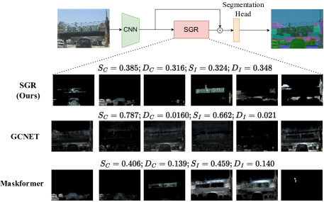
Figure 1: Semantic Global Reasoning. Illustrated is our proposed SGR approach to semantic segmentation (top schematic). Given a feature map from a backbone (ResNet), SGR learns to group pixels into soft semantic latent regions (top); features are aggregated from these regions to form semantic concept token representations that are refined using a Transformer and then back-projected to enhance the original ResNet features, before passing them into segmentation head to produce per-pixel labels. Notably, resulting latent regions are more semantic than prior works, as measured by the proposed class-semantics ($S_{C}$) and instance-semantics ($S_{I}$) measures ($\downarrow$ is better), and are more diverse ($\uparrow$ is better), as measured by proposed class-diversity ($D_{C}$) and instance-diversity ($D_{I}$) (see GCNET [17] / Maskformer [18] in middle/bottom).

Aspirationally, these approaches are motivated by the overarching idea that regions would pull information over individual objects, enhancing pixels with object-centric globally-contextualized representations (e.g., obtained by allowing region representations to interact). In practice, however, this does not happen and visualizations (e.g., such as those in GloRE [17]) show that regions formed in such a manner fail to capture or respect the semantics of the scene. To address this issue, more recent approaches propose to supervise the regions directly. For example, OCR [53] and Maskformer [18] use original semantic mask annotations to supervise the region predictions; class-attention plays a similar role by learning class token embeddings [49]. While these approaches do result in semantic and interpretable regions which improve the performance on the final semantic segmentation task, without requiring any additional supervision, they are still limited in a few key ways.

Mainly, the number of regions is typically limited to the number of semantic classes [18, 53] (in the corresponding dataset) with those regions modeling the union of all object instances in a particular scene. In other words, they are class- and not object-centric. This could be sub-optimal since instances of the same class may have different appearances, or shapes or be located in different disjoint regions of the scene. Aggregating context indiscernibly across them may result in a loss of detail. We posit that a more object-centric aggregation, where regions may be more closely associated with object instances or concepts that compose those instances, and those concept regions would be allowed to aggregate information among them (similar to GloRE [17]) would provide a more granular and interpretable mechanism for attentional context.

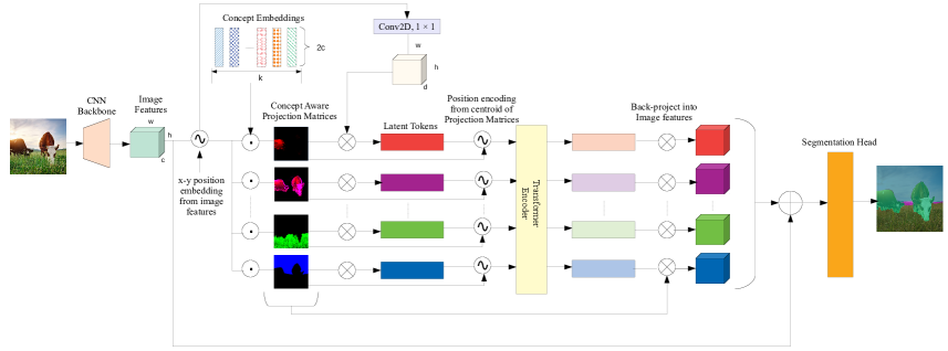
Figure 2: Overview of our framework. An x-y positional embedding is first added to features from the backbone. A dot product is then performed between the position-aware features and $K$ learned concept embeddings to generate soft masks. These masks aggregate features to form latent concept tokens. A transformer encoder learns to enhance these representations using global reasoning through self-attention. Finally, the contextualized output from the transformer is re-projected and added to the feature space and passed to a segmentation head.

The core challenge lies in that one must do so without requiring any instance supervision and relying solely on semantic supervision, similar to prior work. To this end we make the following observations: (1) disconnected semantic segments are likely to belong to different instances – this gives us a lower bound on the number of concept regions per image during training; (2) the union of concept regions for a given class should correspond to its semantic segmentation for that class in a given image; and (3) concept regions must be spatially disjoint. These constraints allow us to formulate a rich set of objective functions that encourage the discovery of concept regions, propagate and refine the representation of those regions in a globally consistent manner, and ultimately enhance the original pixel representation by aggregation of the refined region features. We show that the resulting method not only achieves a competitive performance compared to the state-of-the-art on semantic segmentation but also produces more semantic and diverse regions, as measured by our newly proposed entropy-based metrics. In addition, the more instance-centric nature of the attentional aggregation also ensures that our model learns better underlying feature representations that produce improved performance when transferred to object detection and segmentation tasks.

Contributions.

Our contributions are as follows:

1. We propose a novel framework for semantically-enhanced global reasoning that enhances local feature representations. We do so by learning to form semantic latent regions that pool local information into concept token representations. These latent token representations are then globally refined, using a Transformer [46], and ultimately fused back into the original local feature representations.

2. We propose a rich set of losses that encourage latent regions to be semantically interpretable. Specifically, we ensure that unions of regions map to connected components of ground truth segments; as well as that those regions are disjoint.

3. We define new metrics that measure class- and instance-level semantics of concepts by considering the entropy over ground truth labels that form each corresponding region.

4. We demonstrate that the resulting model, when combined with DeepLabV3 [13], achieves SoTA performance on semantic segmentation in COCO-Stuffs-10K dataset [62] and achieve competitive performance on two other benchmark (Citiscapes [19], and ADE-20K [62]) datasets. In addition, the model results in more semantically interpretable and diverse region representations that leads to improved performance when transferred to the downstream tasks of object detection and segmentation (obtained using Mask R-CNN [25] in MS COCO [37]).

2 Related Work

Semantic Segmentation.

Semantic segmentation is a well-studied problem in computer vision where the goal is to classify each pixel of an image. Earlier approaches required specification of seed points and then used graph cut [42, 5, 4] to group semantically similar features; alternatives generated mask proposals [10, 45, 1, 2] and classified them [9, 20]. With the popularity of deep-learning, focus shifted on converting the segmentation problem to a per-pixel classification problem [12, 40, 13]. Later approaches [13, 14, 15] have shown that capturing more global context leads to improved performance in semantic segmentation. In a shift from per-pixel classification approaches, a recent work, Maskformer [18], goes back to a mask classification approach [9, 20] and uses a transformer [46] to generate mask queries and classify them.

Capturing Global Context.

Earlier approaches attempted to capture the global context in semantic segmentation tasks by either increasing receptive fields [13, 14, 15] using atrous convolution [27, 52, 21] or by aggregating features from multiple scales [60, 15, 51].

Global Reasoning.

Graph-based approaches and self-attention has been extensively used to globally reason between different concepts. CRFs [33, 23] were commonly used in the past for modeling pairwise interaction between all the pixels within an image, particularly to refine predictions [12, 11, 3]. Non-local Nets [47] and variants built a fully connected graph between all the pixels or several sampled pixels [58] and used self-attention over the graph nodes. Recently, a few approaches [17, 35, 59, 48] densely project the image features into latent nodes and then reason between them using graph convolutions [31] or transformers [48, 46]. Although the idea of grouping pixels of similar concepts into regions is similar to ours, visualization of their latent spaces suggests that they fail to capture object semantics at either class or instance level of granularity. To this end, [18, 53] directly supervise latent representations.

Several techniques [24, 28, 54] used different forms of self-attention [46] to obtain the pair-wise relationship between each pixel and aggregate the information to capture the global context for semantic segmentation. Vision Transformers [22] and its variants [39, 61, 43, 8] have tried to generalize self-attention models [46] on many computer vision tasks, including semantic segmentation, with great success, achieving state-of-the-art performance. These models [22, 39, 29, 55] simply divide images into patches and consider them as words similar to language models and use self-attention to reason between them. Subsequent approaches applied shifted windows [39] or clustering [55] to group the patches. Recently DINO [8] observed that the attention maps of class tokens attended to particular regions. However, these maps were class agnostic. MCT [50] exploited this to use multiple class tokens to obtain class-aware attention maps which are refined to be used as pseudo ground truth of semantic segmentation.

3 Method

The motivation for our approach is simple, to enhance local feature representations (e.g., computed by a CNN backbone) with global contextualized scene information. To this end, we introduce a semantically enhanced global reasoning (SGR) component shown in Fig. 2. The input to our component is a convolutional feature map of resolution $W\times H\times C$, where $W$ and $H$ are spatial dimensions and $C$ is the channel dimension. The output is a globally contextualized and enhanced feature map of the same size.

SGR consists of four main steps. First, we divide the image into a set of $K$ soft latent concept regions of size $W\times H$ each. This is achieved by computing the similarity of each input feature column to the learned concept embedding. The representation of the concepts, which ultimately drives the soft concept segmentation, is learned in a weakly-supervised manner where unions of activated concept regions are supervised by connected segments of ground-truth semantic segmentation labels. Second, we form representations for each concept region by aggregating input feature columns corresponding to it. This is similar to context vector aggregation in soft attention and results in a set of $K$ latent semantic token representations. We add positional embeddings corresponding to the centroids of their regions to the token representations [46, 22]. This is important for concept disambiguation (e.g., a low-textured blue token in the lower- and upper-part of the image can be disambiguated, permitting distinctions between sky and water). Third, we perform global reasoning across these semantic tokens by refining their representations using a Transformer [46]. Transformers are effective at capturing global relations among tokens and are more efficient and easier to use than GNNs [17]. Fourth, we fuse information from refined semantic token representations back to the input CNN feature map. This is achieved by back-projecting semantic token representations using the same soft concept regions. Ultimately the result of applying SGR is a refined feature map of original resolution $W\times H\times C$, which is then passed to the segmentation head as shown in Fig. 2.

The key to ensuring the “semanticness” of our concept regions and hence tokens is in the first step where the $K$ concept representations are learned across the dataset. Because we want, ideally, concepts to represent object instances or even parts of object instances, the number of concepts we learn must be a multiple of object classes (unlike [17, 18]). Further, since we do not assume instance-level annotations, we use connected components over the ground truth semantic segmentation annotations to provide a lower bound to the number of concepts that should be active in a given training image. We assume that a subset of $L$ (out of $K$) concepts can be active in each image and guide the learning of concept representations by matching concept regions to the class-specific connected components using a greedy matching strategy (similar to MDETR [30]). Since the connected components are the lower bound, the matching from concepts to connected components is many-to-one. The supervision is such that the union of the concepts is encouraged to correspond to the connected component mask. To ensure that concepts matched to the same connected component are not identical, we force the concept regions corresponding to those tokens to be dissimilar by minimizing pairwise cosine similarity measure.

In what follows we will detail each of our design choices as well as the metrics we defined to measure the semantics of resulting intermediate representations (see Section 4).

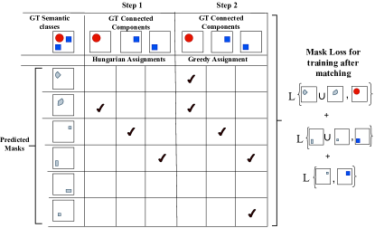
Figure 3: Visualization of our greedy matching strategy. Binary mask losses are used to compute a cost matrix, based on which, Hungarian matching is applied to perform 1-to-1 matching between the predicted latent region masks and the ground truth components. In the second step, we greedily select $L$-top matches from the remaining ones. Once matched, during training, we compute losses between the union of predicted masks assigned to the same ground truth component.

3.1 Projection to Latent Concept Regions

The process of mapping image features into latent regions is illustrated in Figure 2. Given input feature map from a CNN backbone (e.g., ResNet101) $\mathbf{X}\in\mathbb{R}^{W\times H\times C}$, where $W$, $H$ and $C$ are width, height and number of channels respectively, we first add positional embeddings $PE_{pos}(X)$ and $PE_{pos}(Y)$. This is done by computing sines and cosines of different frequencies for $x$- and $y$- index of each feature cell [46], where $PE_{pos}(x)\in\mathbb{R}^{C}$. The result is positionally aware local feature tensor is:

$$\mathbf{X}^{\prime}=\left[\begin{array}[]{c}\mathbf{X}+PE_{pos}(X)\\ \mathbf{X}+PE_{pos}(Y)\\ \end{array}\right],$$ (1)

where $\mathbf{X}^{\prime}\in\mathbb{R}^{W\times H\times 2C}$. We obtain the latent concept regions by computing dot product similarity of each feature cell of $\mathbf{X}^{\prime}$ with learned concept embeddings $\mathbf{b}_{k}\in\mathbb{R}^{2C}$; $k\in[1,K]$, where $K$ is the total number of concepts. This results in $K$ soft masks of resolution $W\times H$, collectively forming $\mathbf{P}=[\mathbf{P}_{1},\mathbf{P}_{2},...,\mathbf{P}_{K}]\in\mathbb{R}^{W\times H\times K}$. In practice, the above operation is implemented by a 2D convolution with $K$ kernels of $1\times 1$:

$$\mathbf{P}=\text{\tt sigmoid}(\text{\tt Conv2D}(\mathbf{X}^{\prime};\{\mathbf{b}_{k}\}_{k=0}^{K})).$$ (2)

3.2 Projection to Latent Semantic Tokens

We use another convolution layer with $1\times 1$ kernels to reduce the dimensionality of $\mathbf{X}^{\prime}$ to $\mathbb{R}^{H\times W\times D}$. The latent semantic tokens for the $K$ regions are formed by matrix multiplication between the dimensionally reduced positional features and obtained soft concept region masks. This is facilitated by flattening both tensors along the first two dimensions and element-wise multiplying across channel dimensions of the $D$-dimensional features:

$$\mathbf{T}=\mathbf{P}^{T}\odot\text{\tt Conv2D}(\mathbf{X}^{\prime};\mathbf{W}_{d})^{T}.$$ (3)

3.3 Global Reasoning Between the Tokens

After projecting features into latent tokens, we add positional encoding for the location of the tokens themselves into their respective representations. We characterize the position of the token by a weighted centroid computed by its soft concept region mask. Mainly, $\mathbf{T}^{\prime}=\mathbf{T}+PE_{pos}(\mathbf{C})$, where

$$\mathbf{C}_{k}=\frac{1}{\sum_{i}\sum_{j}\mathbf{P}_{i,j,k}}\sum\limits_{w=1}^{W}\sum\limits_{h=1}^{H}\left[w\mathbf{P}_{w,h,k};h\mathbf{P}_{w,h,k}\right].$$ (4)

The tokens with positional encoding, $\mathbf{T}^{\prime}$, are passed on as inputs to the transformer [46].

The transformer applies self-attention over the tokens thereby performing global communication between them. Because each token represents a component of a semantic class, it only pulls features from the semantic concept or component it represents. Overall, this self-attention-based reasoning is analogous to identifying the relationships between different semantic concepts at different locations.

The output of the transformer is then back-projected onto the pixel space using the same projection matrix that we used to project the original features to the latent space. The back-projected features are added with the input features and passed to segmentation head for per-pixel classification.

3.4 Latent Concept Supervision

We aim to make each token semantic, such that it only aggregates features from the component of the semantic class (ideally an instance, but possibly a part of the instance of an object) it represents. For example, we would like to have concepts that represent each car in a scene, but would also be happy with concepts that separately represent each car’s wheels and body.

We observe that disconnected components of the semantic segments for a given object class are likely to belong to different instances and hence they should correspond to different concepts as per the construction above. Hence, during training, we first apply connected component analysis over the binary ground truth segmentation masks to obtain the connected components of each semantic class. We use the resulting connected components to supervise soft latent concept region masks. At training time, we first match the predicted latent concept masks of each token to these connected components based on a cost matrix. Once matched, we supervise the projection matrices using the ground truth connected component masks to ensure that concept tokens are only formed from from a particular class component.

Specifically, given $K$ soft latent concept region masks, we assume that only up to $L$ of them are active in any given image and must be matched to $C$ ground truth connected components. We assume $K>L>C$ (for example in most experiments we let $K=256$ and $L=64$). We first form a $K\times C$ cost matrix and then obtain matching using a two-stage procedure. First, we use the Hungarian algorithm [34, 18, 7] to perform a bipartite matching between ground truth connected components and latent concept region masks. This ensures that each connected component is associated with at least one latent concept region. Second, we match the remaining $L-C$ latent concept regions greedily to connected components by considering the remaining $(K-C)\times C$ portion of the cost matrix. The procedure is illustrated in detail in Figure 3.

The key to the above procedure is the formation of the cost matrix. Each $(i,j)$-th entry in the cost matrix measures similarity between the $i$-th soft latent concept region mask $\mathbf{P}_{i}$ and the binary ground truth mask for a connected component $\mathbf{M}_{j}$ of one of the classes present in the given image. To measure similarity we use a combination of dice loss [41] and focal loss [36],

$$Cost_{i,j}(\mathbf{M}_{j})=\mathcal{L}_{focal}(\mathbf{P}_{i},\mathbf{M}_{j})+\rho\mathcal{L}_{dice}(\mathbf{P}_{i},\mathbf{M}_{j}).$$ (5)

The hyperparameter $\rho$ controls the relative weight of the two terms in the cost computation.

Once the tokens are matched, we can supervise them using the same losses used to match them. However, since we have many-to-one matching between latent concept regions and ground-truth connected components this results in tokens that are duplicates of one another. To avoid this scenario we add regularization which ensures that latent regions compete for support. This is achieved using cosine similarity loss that is applied to pairs of latent concepts that are matched to the same connected component: $\mathcal{L}_{cos}(\mathbf{P}_{i\rightarrow j},\mathbf{P}_{k\rightarrow j})$. The final loss for supervision of latent concepts can be written as follows:

$$\mathcal{L}_{concept}(\mathbf{P},\mathbf{M})=\sum\limits_{j=1}^{C}\mathcal{L}_{focal}(\sum\limits_{i\rightarrow j}\mathbf{P}_{i},\mathbf{M}_{j})+\\ \rho\sum\limits_{j=1}^{C}\mathcal{L}_{dice}(\sum\limits_{i\rightarrow j}\mathbf{P}_{i},\mathbf{M}_{j})+\gamma\sum\limits_{i=1}^{L}\sum\limits_{k=1}^{L}\mathcal{L}_{cos}(\mathbf{P}_{i\rightarrow j},\mathbf{P}_{k\rightarrow j}).\vspace{-6pt}$$ (6)

Note that with a slight abuse of notation the sums in the focal and dice losses are overall concept regions $i$ that matched to one connected component $j$, and are effectively modeling the union of the concept regions matched to a given component (see Figure 3 (right)). This, in effect means that concepts are only weakly-supervised. The $\rho$ and $\gamma$ are the balancing parameters for the loss terms.

3.5 Final Loss

The final loss for our model is a combination of the traditional per-pixel supervised classification loss and the latent concept loss defined above. In other words, we optimize:

$$\mathcal{L}=\mathcal{L}_{CE}(\cdot,\cdot)+\beta\mathcal{L}_{concept}(\mathbf{P},\mathbf{M}),$$ (7)

where $\mathcal{L}_{CE}$ is a typical per-pixel cross-entropy loss and we omit parameters to avoid notation clutter. Again, $\beta$ is a balancing parameter between the two terms.

4 Metrics for interpretability

Our goal is not only to obtain an effective segmentation model but to do so with latent region representations that are semantic. Hence we propose a series of metrics that measure the semantics of representations. Our metrics rely on two core assumptions: (1) the token is semantic if its latent region belongs to a coherent (object class or instance), and (2) latent regions, as a collection, should capture as many object categories and instances as possible (i.e., be diverse).

Class-Semantics ($\mathcal{S}_{C}$). To measure semantics, we first compute a histogram for each token of ground truth object classes that lay within its latent support region. We do so by forming a histogram where bins correspond to the classes present in the image. Each pixel soft votes for the label of its labeled ground truth object class with the soft weight assigned to it by the token. The histogram is then normalized to sum to 1. In effect, for each image, we compute $K$ discrete probability distributions that measure the empirical probability of the object class belonging to the token. We measure the entropy of these probability distributions and then average the resulting K entropies. We take this mean entropy as the measure of the semantics of token representations for the given image. Note, the lower the entropy the more semantic the token representations are because a lower entropy indicates a uni-modal distribution suggesting that most of the token support comes from a single object class. A dataset measure can be obtained by averaging mean entropy over all images.

Instance-Semantics ($\mathcal{S}_{I}$). We extend this metric to quantify the ability of our tokens to distinguish between individual object instances and not just classes. In this case, we make the bins of the histogram correspond to the individual instances for each of the ”things” classes (a class that has instance annotations). The rest of the metrics can be computed in the same way. We note that having a desirable low value for instance-semantics will inherently lead to a low value for class-semantics, but not vice versa.

Diversity. One can minimize the semantics metric above by having all tokens focus on only one object class or instance. Hence it is desirable to also measure diversity of representations. To quantify the diversity of our tokens, we propose the token diversity metric. To compute this metric, we first compute the mean of the normalized histograms mentioned above. Then we measure the variance of the histograms for an image. Finally, we compute the mean of these variances for the entire dataset. The higher the variance, the more diverse the tokens are. We desire a high token diversity. Similar to semantics, diversity can also be defined at the class- or instance level. For the rest of the paper, we refer to class-level token diversity as ($\mathcal{D}_{C}$) and instance-level token diversity as ($\mathcal{D}_{I}$).

5 Experiments

To show the effectiveness of our SGR framework we have experimented with three widely used semantic segmentation datasets: Cityscapes [19], COCO-Stuffs-10k [6] and ADE-20K [62]. We add our SGR unit just before the segmentation head of DeepLabV3 [14] semantic segmentation network. We then conduct three sets of experiments: (1) experiments on semantic segmentation where we show that the resulting method achieves SoTA performance on all three datasets (ranking 1-st on one dataset and 2-nd on the other two); (2) experiments that compare semantics and diversity of our resulting representations with recent alternatives GCNET [17] and Maskformer [18], where we show superiority of our representations. Finally, (3) we demonstrate the effectiveness of the features learned by our global reasoning component, by transferring the learned weights from the semantic segmentation network and fine-tuning to downstream tasks like object detection and instance segmentation on the MS-COCO dataset [37]. We also carried out a series of ablation studies to justify our design choices.

5.1 Datasets

Cityscapes [19] contains high-resolution images of street-view in different European cities captured using a dashcam. There are 2975 images for training, 500 for validation, and 1525 images for testing. It has 19 semantic classes labeled.

COCO-Stuffs-10K [6] is a subset of the MS-COCO dataset [37] commonly used for semantic segmentation. It has pixel-level annotations of 171 semantic classes of which there are 80 “things” and 91 “stuffs” classes. There are 9K images (varying resolution) for training and 1K for testing.

ADE-20K [62] is a subset of the ADE20K-Full dataset containing several indoor and outdoor scenes with 150 semantic classes. It contains around 20K images for training and 2K images for validation of varying resolutions.

MS-COCO [37] is a large-scale dataset used for object detection, segmentation, and image captioning.

5.2 Implementation Details

Semantic Segmentation.

For semantic segmentation, we add our SGR component after the final layer of the ResNet [26] backbone, pre-trained on ImageNet, just before the segmentation head of DeepLabV3 [14]. DeepLabV3 uses a multi-grid approach with dilated convolutions during training. The last two downsampling layers are removed resulting in an output stride of 8. We use the SGD optimizer with a momentum of 0.9 [44] and a polynomial learning rate policy where the learning rate decreases with the formula $(1-\frac{iter}{total\_iter})^{0.9}$. For Cityscapes [19], we use a batch size of 8 and a crop size of $768\times 768$ with an initial base learning rate of 0.006. For both Coco-Stuffs [6] and ADE-20K [62] we use a batch size of 16, crop size of $512\times 512$ and an initial base learning rate of 0.004. For all our experiments, we multiply the initial base learning rate by 10.0 for the parameters of our SGR component and the layers that correspond to the segmentation head. We train Cityscapes, COCO-Stuffs-10K, and ADE-20K for 240 epochs, 140 epochs, and 120 epochs respectively. We report both the single-scale inference and multi-scale inference with a horizontal flip at scales 0.5, 0.75, 1.0, 1.25, 1.5, and 1.75 following existing works [53, 18, 24, 14].

Transfer to Downstream Tasks.

To show the effectiveness of the features learned by our framework, we transfer the model learned on the semantic segmentation task to object detection and segmentation. We first remove the segmentation head from our semantic segmentation network trained on COCO-Stuffs-10K and use it as a backbone for Mask-RCNN [25] to fine-tune on MS-COCO for object detection and instance segmentation. We trained our model on MS-COCO train2017 which has 118K images and evaluated on val2017 which has 5K images. For a fair comparison with other backbones, we trained with the same batch size, learning rate, and iterations. We used a batch size of 8, an initial learning rate of 0.02, and used SGD with a momentum of 0.9 and weight decay of 0.0001 to train the models. We trained for 270K iterations with a learning rate decreased by 0.1 at 210K and 250K iterations.

Additional details are given in Supplemental.

5.3 Results

Semantic segmentation.

The performance of our approach on semantic segmentation is shown in Table 1. As can be observed, our model obtains competitive performance across all three datasets compared to the state-of-the-art (SoTA) models that use the ResNet backbone. We achieve SoTA for COCO-Stuffs-10K [6] in both single- (s.s.) and multi-scale (m.s.) settings. On ADE-20K our approach achieves second best performance followed by Maskformer [18]. However, unlike other approaches that use Resnet-101, they use an FPN-based pixel decoder which increases the output stride to $4\times$. On the Cityscapes validation set, we also obtain a competitive result (third on s.s.; second on m.s. settings). However, Cityscapes only has 19 semantic classes which are not evenly balanced (in terms of a number of pixels and presence in the dataset) compared to 150 and 171 semantic classes for ADE-20K and COCO-Stuffs respectively. As argued by Maskformer [18], we also observe that our global reasoning benefits from having a greater number of semantic classes and diversifies the type of tokens among which the transformer can reason.

Models	Backbone	O.S.	Datasets	mIoU (s.s.)	mIoU (m.s.)
DL-V3 [14]	ResNet-101	$8\times$	COCO-Stuffs-10K	37.4	38.6
GCNET (DL-V3 + GloRE) [17]	ResNet-101	$8\times$	COCO-Stuffs-10K	37.2	38.4
DANET [24]	ResNet-101	$8\times$	COCO-Stuffs-10K	-	39.7
OCRNet [53]	ResNet-101	$8\times$	COCO-Stuffs-10K	38.4	39.5
Maskformer [18]	ResNet-101	$\mathbf{4\times}$	COCO-Stuffs-10K	38.0	39.3
Ours (DL-V3 + SGR)	ResNet-101	$8\times$	COCO-Stuffs-10K	38.8	39.7
DL-V3 [14]	ResNet-101	$8\times$	ADE-20K-val	42.9	44.0
GCNET (DL-V3 + GloRE) [17]	ResNet-101	$8\times$	ADE-20K-val	43.2	44.8
DANET [24]	ResNet-101	$8\times$	ADE-20K-val	-	45.2
OCRNet [53]	ResNet-101	$8\times$	ADE-20K-val	-	45.3
Maskformer [18]	ResNet-101	$\mathbf{4\times}$	ADE-20K-val	45.5	47.2
Ours (DL-V3 + SGR)	ResNet-101	$8\times$	ADE-20K-val	43.8	45.6
DL-V3 [14]	ResNet-101	$8\times$	Cityscapes-val	78.0	79.3
GCNET (DL-V3 + GloRE) [17]	ResNet-101	$8\times$	Cityscapes-val	77.9	79.4
DANET [24]	ResNet-101	$8\times$	Cityscapes-val	79.9	81.5
OCRNet [53]	ResNet-101	$8\times$	Cityscapes-val	79.6	-
Maskformer [18]	ResNet-101	$\mathbf{4\times}$	Cityscapes-val	78.5	80.3
Ours (DL-V3 + SGR)	ResNet-101	$8\times$	Cityscapes-val	78.7	80.5

Table 1: Results for semantic segmentation. For Cityscapes and ADE-20K the results are reported on the validation set, while for COCO-Stuff-10K the results are reported on the test-set. B, R and G represents best, second best and third best respectively.

Models	Backbone	$\mathbf{K}$	Datasets	$\mathcal{S}_{C}$$\downarrow$	$\mathcal{D}_{C}$$\uparrow$
GCNET (DL-V3 + GloRE) [17]	ResNet-101	64	COCO-Stuffs-10K	0.478	0.078
Maskformer [18]	ResNet-101	100	COCO-Stuffs-10K	0.275	0.186
Ours (DL-V3 + SGR)	ResNet-101	512	COCO-Stuffs-10K	0.226	0.389
GCNET (DL-V3 + GloRE) [17]	ResNet-101	64	ADE-20K-val	0.564	0.106
Maskformer [18]	ResNet-101	100	ADE-20K-val	0.335	0.173
Ours (DL-V3 + SGR)	ResNet-101	512	ADE-20K-val	0.264	0.391
GCNET (DL-V3 + GloRE) [17]	ResNet-101	64	Cityscapes-val	0.741	0.055
Maskformer [18]	ResNet-101	100	Cityscapes-val	0.413	0.209
Ours (DL-V3 + SGR)	ResNet-101	256	Cityscapes-val	0.293	0.469
Models	Backbone	$\mathbf{K}$	Datasets	$\mathcal{S}_{I}$ $\downarrow$	$\mathcal{D}_{I}$  $\uparrow$
Maskformer [18]	ResNet-101	100	MS-COCO	0.383	0.122
Ours (DL-V3 + SGR)	ResNet-101	512	MS-COCO	0.315	0.316

Table 2: Semantics. Comparison of class-level ($\mathcal{S}_{C}$) and instance-level ($\mathcal{S}_{I}$) semantics of intermediate tokens and the token diversity on class ($\mathcal{D}_{C}$) and instance-level ($\mathcal{D}_{I}$). The lower the value of ($\mathcal{S}_{C}$) and ($\mathcal{S}_{I}$) the more semantic the the token representations are.

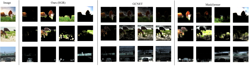
Figure 4: Qualitative results showing that our SGR component generates a more semantically meaningful and diverse tokens. In all three images, SGR was able to disambiguate between the instances (was able to differentiate the cow in the left in the first image, and different groups/ instances of the car in the last row) unlike Maskformer [18]. GCNET [17] tokens, on the other hand, lack strong semantic meaning.

Class and instance-semantics.

We quantify the interpretability of the generated tokens for SGR at the class-level and instance-level using the metrics discussed in Section 4 and compare against intermediate representations of Maskformer [18] and tokens of GLoRE [17]. The results are shown in Table 2. $\mathcal{S}_{C}$ and $\mathcal{S}_{I}$ denotes class-level and instance-level semantics respectively while $\mathcal{D}_{C}$ and $\mathcal{D}_{I}$ indicates token diversity at class and instance level. As can be observed, our tokens are more semantically meaningful than other intermediate representations at both semantic and instance levels while at the same time being more diverse. As mentioned in Section 4, a lower semantics value at the class level or instance level means that the token only aggregates information from that particular class or instance. A higher diversity ensures that our tokens aggregate information from diverse classes and instances. For instance-semantics, we reported results on MS-COCO because COCO-Stuffs does not have instance annotations, while the models themselves are trained on COCO-Stuffs.

Backbone	$AP_{bbox}$	$AP_{50}$	$AP_{75}$	$AP_{S}$	$AP_{M}$	$AP_{L}$
Res101-C4 [26, 25]	40.29	59.58	43.37	22.41	44.94	55.05
Res101-GCNET [17]	38.85	58.82	42.30	21.62	42.76	51.88
Ours-Res101-SGR	41.91	62.79	45.23	22.95	46.04	56.32
Ours (w/o token sup.)	33.48	51.72	36.2	18.73	36.96	45.84

Table 3: Transfer to Object Detection. Results showing transfer learning performance on object detection using Mask-RCNN [25]. All the models are initialized with corresponding pre-trained backbone and then trained on COCO train2017 by us and evaluated on val2017 for a fair comparison.

Backbone	$AP_{mask}$	$AP_{50}$	$AP_{75}$	$AP_{S}$	$AP_{M}$	$AP_{L}$
Res101-C4	34.88	56.16	37.27	15.30	38.32	53.18
Res101-GCNET	34.35	55.08	36.43	15.07	38.33	51.37
Ours-Res101-SGR	37.06	59.28	39.31	16.30	40.95	56.19
Ours (w/o token sup.)	29.73	48.75	31.41	13.55	33.85	46.41

Table 4: Transfer to Instance Segmentation. Results showing transfer learning performance on object segmentation using Mask-RCNN [25]. All the models are initialized with corresponding pre-trained backbone and then trained on COCO train2017 by us and evaluated on val2017 for a fair comparison.

		COCO-Stuffs-10K			MS-COCO
Backbone	Method	mIOU(m.s.)	$\mathcal{S}_{C}$$\downarrow$	$\mathcal{D}_{C}$$\uparrow$	$\mathcal{S}_{I}$ $\downarrow$	$\mathcal{D}_{I}$  $\uparrow$
Res-101	token sup.	39.7	0.226	0.389	0.315	0.316
Res-50	token sup	37.1	0.235	0.371	0.331	0.306
Res-101	w/o token sup.	38.6	0.556	0.001	0.640	0.001

Table 5: Ablation Studies on COCO-Stuffs-10K. mIOU and class-semantics reported on COCO-Stuffs-10K. Instance semantics and instance diversity are reported on COCO val2017. All models for ablation studies are trained on COCO-Stuff-10K-train. ($\mathcal{S}_{C}$) and ($\mathcal{S}_{I}$) represent class and instance semantics respectively while ($\mathcal{D}_{C}$) and ($\mathcal{D}_{I}$) – class and instance-level token diversity.

Transfer to downstream tasks. Tables 3 and 4 show the performance of our proposed component when transferred to down-stream tasks of object detection and segmentation on MS-COCO [37] dataset using Mask-RCNN [25]. We compared against two other backbones, Resnet-101 (Res101-C4) pre-trained on Imagenet and GloRE (Res101-GCNET) [17] pre-trained on COCO-Stuffs-10K on semantic segmentation task. As can be observed from Table 3 and 4, SGR outperforms both on object detection and instance segmentation tasks. This demonstrates that the more semantically interpretable and diverse token representations allow us to learn richer features that are broadly more useful and transferable. Note that these downstream tasks require the ability to discern multiple instances and the instance-centric nature of the way our SGR aggregates information allows us to achieve this improved performance. This is further highlighted when compared against the model transferred from GloRE [17] which also aggregates features into multiple tokens and reasons between them but the tokens lack any semantic coherence.

Ablation Studies.

The last row of Tables  3 and 4 further highlights the importance of our approach of supervising tokens to aggregate semantically meaningful regions. As shown in those tables, when we train our SGR model on COCO-Stuffs-10K without using token supervision, the performance on downstream tasks drastically drops. Table 5 shows the semantic segmentation performance of our method on a different backbone (Resnet-50) and the corresponding class and instance semantics and diversity. As can be observed, even when we use a weaker backbone, our model can retain the semantics on both class and instance-level reasonably well and produces diverse tokens. We further report the performance of SGR when the tokens are not supervised to be semantically meaningful. Not only does the semantic segmentation performance deteriorate, but the tokens are no longer semantically meaningful (as expected).

Qualitative Results. Figure 4 shows qualitative results for generated tokens on multiple images. As can be observed, our tokens are more semantically interpretable and diverse, compared to the GCNET [17] and Maskformer [18]. Crucially, compared to Maskformer, which also supervises tokens, SGR can distinguish between instances of objects at different spatial locations; e.g., in the first row, one of the tokens of SGR is able to distinguish the left cow from the other, while Maskformer [18] fails to do so. We can similarly observe that SGR is able to distinguish the rightmost horse in the second image which is disjoint from the rest and in the last image three different tokens of SGR are attending to three different groups of cars where other methods failed.

6 Conclusion

To summarize, we propose a novel component that learns to semantically group image features into latent tokens and reasons between them using self-attention. The losses we propose allow our latent representations to distinguish between individual connected components of a semantic class. We also propose new metrics to demonstrate that our latent tokens are meaningful and semantically interpretable at both class- and instance-levels. Moreover, we achieve competitive performance compared to the state-of-the-art using CNN backbones on semantic segmentation. We have also demonstrated that we learn a rich set of features that can be transferred to downstream object detection and instance segmentation tasks.

Acknowledgments

This work was funded, in part, by the Vector Institute for AI, Canada CIFAR AI Chair, NSERC CRC and an NSERC DG and Accelerator Grants. Hardware resources used in preparing this research were provided, in part, by the Province of Ontario, the Government of Canada through CIFAR, and companies sponsoring the Vector Institute. Additional support was provided by JELF CFI grant and Compute Canada under the RAC award. Finally, we sincerely thank Gaurav Bhatt for his valuable feedback and help with the paper draft.

Supplementary Material

1 Implementation Details

1.1 Semantic Segmentation

As mentioned in our main paper, for semantic segmentation, the SGR component is added after the final layer of the ResNet [26] backbone, pre-trained on ImageNet, just before the segmentation head of DeepLabV3 [14]. DeepLabV3 uses a multi-grid approach with dilated convolutions during training. The last two downsampling layers are removed resulting in an output stride of 8. The models are trained using the SGD optimizer with momentum [44] of 0.9 with a weight decay of 0.0001. We used a polynomial learning rate policy where the learning rate decreases with the formula $(1-\frac{iter}{total\_iter})^{0.9}$ with every iteration.

During training, we applied random horizontal flips, random scaling between [0.5-2.0] and random color jitter following [53, 18] for data augmentation. For cityscapes [19], following the random data augmentation, the images are cropped from the center with a crop size of $768\times 768$. For both ADE-20K [62] and Coco-Stuffs-10K [6] a center crop of crop size $512\times 512$ is used following the above mentioned random image transformations during training.

The model on cityscapes [19] is trained with a batch size of 8 and an initial learning rate of 0.006. The models on ADE-20K [62] and Coco-Stuffs-10K [6] are trained with a batch size of 16 and an initial learning rate of 0.004. For all three datasets, the initial base learning rate is multiplied by a factor of 10.0 for the parameters of the SGR component and the layers that correspond to the segmentation head. When trained across multiple GPUs, we apply synchronized batchnorm [57] to syncrhonize batch statistics following existing work [14, 24, 17, 53, 18]. We train Cityscapes, COCO-Stuffs-10K, and ADE-20K for 240 epochs, 140 epochs and 120 epochs respectively.

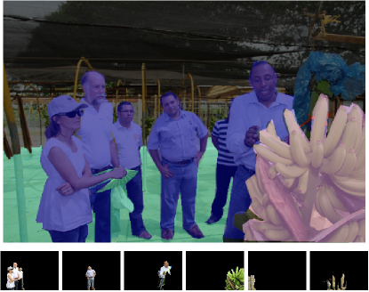
Figure 5: Ground truth segmentation mask and corresponding connected components. The connected components are assumed to give a lower bound on the number of instances; e.g., illustrated image contains 6 people but the number of connected components that corresponds to person is only 3.

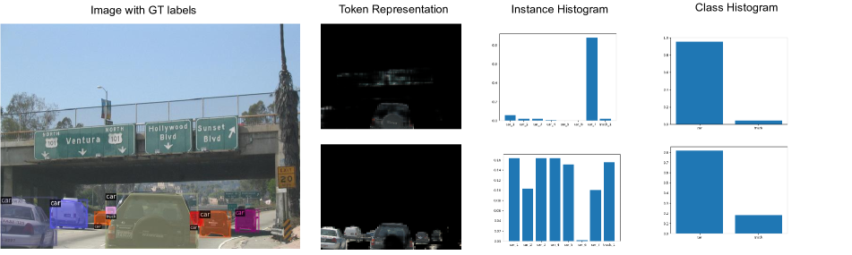
Figure 6: Visualization of instance- and class-level histograms. (Left) Image with ground truth instances of ”things” classes. (2nd Column) Two different token projection matrices aggregating information from different concepts. (3rd Column) Instance-level histograms. (Right) Class-level histograms. Even though the bottom token captures a good class-level semantics (mostly aggregating features of cars), on instance-level the semantics are poor.

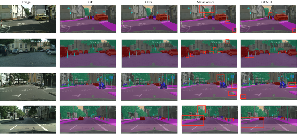
Figure 7: Qualitative results on Citscapes. Leftmost two columns correspond to the image and ground truth semantic segmentation; Center column shows the predictions of our model; Rightmost two columns show predictions from Maskformer [18] and GloRE [17]. Red rectangles on the images of two rightmost columns indicate locations where our model correctly classifies semantic classes but the corresponding models fail.

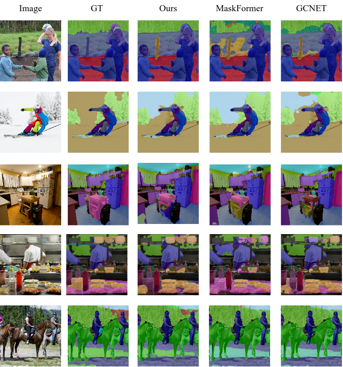
Figure 8: Qualitative results on COCO-Stuffs-10K. Leftmost two columns correspond to the image and ground truth semantic segmentation; Center column shows the predictions of our model; Rightmost two columns show predictions from Maskformer [18] and GloRE [17].

Figure 9: Qualitative results for downstream tasks of object detection and instance segmentation on MS-COCO. Leftmost two columns correspond to the image and ground truth object locations and their corresponding segmentation; Center column shows the predictions of using our backbone; Rightmost two columns show predictions from using Res101-C4 and Res101-GloRE [17] backbones.

For all three datasets, we report both the single scale inference and multi-scale inference with horizontal flip at scales 0.5, 0.75, 1.0, 1.25, 1.5 and 1.75 following existing works [53, 18, 24, 14]. During multi-scale inference, the final output is calculated by taking the mean probabilities over each scale and their corresponding flipped inputs. Following  [24, 53, 18], for ADE-20K and COCO-Stuffs, we resize the shorter side of the image to the crop size followed by a center crop to ensure that all images are of same size.

Hyper-parameters for training. For Hungarian matching, in training, we used a $\rho=1.0$ for dice loss (see Eq. (5) in the main paper). For matching, as mentioned in the paper, the value of $L$ is set to 64. Hence, the top $L=64$ tokens are matched using the greedy matching approach based on the cost matrix (Figure 3 of the main paper). Once matched, we used a weight of 0.25 for the hyperparameter $\beta$ that controls the importance of binary mask losses with respect to cross-entropy loss to train the models (see Eq. (7)).

1.2 Transfer to Downstream Tasks

For transferring to the downstream tasks, we removed the segmentation head from our semantic segmentation network trained on COCO-Stuffs-10K and use it as a backbone for Mask-RCNN [25] to fine-tune on the MS-COCO train2017 subset, which has 118K images, for object detection and instance segmentation. The same approach was adopted while transferring the GloRE [17] based backbone pretrained for segmentation on COCO-Stuffs-10K. For the Res101-C4 backbone however, we used the weights pretrained for classification on Imagenet. We reported our results on val2017 subset having 5K images. The authors of Mask-RCNN used a batch size of 16 and trained on the trainval-135K subset and reported results on the minival dataset which is the same as val2017. Therefore, for a fair comparison with other backbones, we trained them from scratch on MS-COCO train2017 using the same batch size, learning rate and iterations. We used a batch size of 8, an initial learning rate of 0.02, and used SGD with a momentum of 0.9 and weight decay of 0.0001 to train the models. We trained for 270K iterations with a learning rate decreased by 0.1 at 210K and 250K iterations. Following Mask-RCNN [25], the RPN anchors span 5 scales and 3 aspect ratios. For all the reported backbones, 512 ROIs are sampled with a positive to negative ratio 1:3.

At inference time, we used 1000 region proposals for all the three backbones. Following Mask-RCNN [25], the box predictions are performed on these region proposals and top 100 scoring boxes are chosen by non-maximum suppression on which the mask predictor is run.

2 Ground Truth connected components

Figure 5 shows the result of applying connected component analysis on ground truth semantic segmentation masks. As can be seen in the figure, the class person is divided into three different components. There are altogether 6 people in total. Hence, we observe that generally connected components form a lower bound on the number of instances. Similarly, the “stuffs” class ground is divided into two different components and the class banana has only one component. For “stuffs” classes the notion of instances is not well defined, but yet connected components serve as a good proxy for disjoint regions that are often semantically meaningful within the scene.

3 Visualization of histograms for tokens

Figure 6 shows the visualization of class-level and instance-level histograms for two different tokens, which we use to compute class- and instance-level semantics metric (defined in the main text). The lower the entropy of each of these histograms, the more semantically meaningful the tokens are at class or instance level of granularity. As can be observed in Figure 6, the first token has high instance and class level semantics since it mostly aggregates information from a single car, in this case, car_7. The lower token, despite being highly semantic at class-level (having lower entropy at class-level), is poor at capturing instance-level semantics. Hence, a token which is semantic at an instance-level is also highly semantic at class-level but not the other way around.

4 Qualitative Results

4.1 Semantic Segmentation

Qualitative Results on Cityscapes. Figure 7 shows qualitative results of semantic segmentation of our model on Cityscapes compared to Maskformer [18] and GCNET [17]. The red rectangles indicate locations where our model performs better than others; e.g., in the first image, Maskformer has miss-classified sky for another class. GCNET has miss-classified the pavement (as shown by red rectangle in the rightmost corner) and a road sign in the middle.

Qualitative Results on COCO-Stuffs-10K Figure 8 shows the qualitative result of semantic segmentation of our model on COCO-Stuffs-10K compared to Maskformer [18] and GloRE [17]. For the first image, the predictions of our model are clearly more accurate, compared to the other two models. In the second image, all three models miss-classified the snow for sky to some extent. However, Maskformer has greater miss-classification of snow as sky compared to the rest. GCNET, on the other hand, overestimated the region of trees and had lower mIOU for skis, but has slightly better classification on snow. In the third image, Maskformer has completely miss-classified the microwave and GCNET incorrectly classified the table in the center and the bottles on top of the shelves. In the fourth image, we clearly do a better job at correctly predicting the segments, compared to the rest. In the last image, two competing models failed to classify the mountains correctly. They also miss-classified gravel road which our model correctly classified.

4.2 Object Detection and Instance Segmentation

Figure 8 shows the qualitative result of object detection and instance segmentation of using our pre-trained backbone in Mask-RCNN [25] on MS-COCO, compared to pre-trained Res101-C4 and Res101-GloRE [17] backbones. In the first image, the other two backbones, miss-classified the leftmost elephant as a person which we correctly identify and segment. Moreover, they missed the rightmost instance of the elephant which model using our backbone was able to detect. Overall segmentation quality of each elephant was also better for our backbone. In the second image, other backbones erroneously classified the lamp on the left as parking meter. This is likely due to the lack of global reasoning needed to make a distinction between these two objects within the context of the scene that our backbone contains. Both of them also missed backpack of the person on the right. Our backbone equipped model, consistently identifies objects and segments them better.

In the third image, our backbone segments the couches better than the other backbones. In the fourth image, the instance segmentation of the person is better than the other two backbones. Moreover, Res101-C4 backbone has missed the handbag altogether, while Res-101-GloRE backbone cannot segment the handbag properly. In the final image, Res-101-C4 backbone incorrectly labelled US flag as a chair. Besides the instance segmentation quality is lower than our backbone. The Res-101-GloRE failed to identify the truck completely, identifying part of of it as motorcycle and inaccurately segmented it. The general quality of object segmentation is also worse. All these qualitative results demonstrate the fact that our SGR component, due to instance-like supervision through connected components, learns richer features that when transferred to downstream tasks improves performance in object detection and instance segmentation.

References

- [1] Pablo Arbeláez, Bharath Hariharan, Chunhui Gu, Saurabh Gupta, Lubomir Bourdev, and Jitendra Malik. Semantic segmentation using regions and parts. In CVPR, pages 3378–3385. IEEE, 2012.
- [2] Pablo Arbeláez, Jordi Pont-Tuset, Jonathan T Barron, Ferran Marques, and Jitendra Malik. Multiscale combinatorial grouping. In CVPR, pages 328–335, 2014.
- [3] Gedas Bertasius, Lorenzo Torresani, Stella X Yu, and Jianbo Shi. Convolutional random walk networks for semantic image segmentation. In CVPR, pages 858–866, 2017.
- [4] Yuri Boykov and Gareth Funka-Lea. Graph cuts and efficient nd image segmentation. IJCV, 70(2):109–131, 2006.
- [5] Yuri Boykov and Vladimir Kolmogorov. An experimental comparison of min-cut/max-flow algorithms for energy minimization in vision. PAMI, 26(9):1124–1137, 2004.
- [6] Holger Caesar, Jasper Uijlings, and Vittorio Ferrari. Coco-stuff: Thing and stuff classes in context. In CVPR, pages 1209–1218, 2018.
- [7] Nicolas Carion, Francisco Massa, Gabriel Synnaeve, Nicolas Usunier, Alexander Kirillov, and Sergey Zagoruyko. End-to-end object detection with transformers. In ECCV, pages 213–229. Springer, 2020.
- [8] Mathilde Caron, Hugo Touvron, Ishan Misra, Hervé Jégou, Julien Mairal, Piotr Bojanowski, and Armand Joulin. Emerging properties in self-supervised vision transformers. In ICCV, pages 9650–9660, 2021.
- [9] Joao Carreira, Rui Caseiro, Jorge Batista, and Cristian Sminchisescu. Semantic segmentation with second-order pooling. In ECCV, pages 430–443. Springer, 2012.
- [10] Joao Carreira and Cristian Sminchisescu. Cpmc: Automatic object segmentation using constrained parametric min-cuts. PAMI, 34(7):1312–1328, 2011.
- [11] Siddhartha Chandra, Nicolas Usunier, and Iasonas Kokkinos. Dense and low-rank gaussian crfs using deep embeddings. In ICCV, pages 5103–5112, 2017.
- [12] Liang-Chieh Chen, George Papandreou, Iasonas Kokkinos, Kevin Murphy, and Alan L Yuille. Semantic image segmentation with deep convolutional nets and fully connected crfs. arXiv preprint arXiv:1412.7062, 2014.
- [13] Liang-Chieh Chen, George Papandreou, Iasonas Kokkinos, Kevin Murphy, and Alan L Yuille. Deeplab: Semantic image segmentation with deep convolutional nets, atrous convolution, and fully connected crfs. PAMI, 40(4):834–848, 2017.
- [14] Liang-Chieh Chen, George Papandreou, Florian Schroff, and Hartwig Adam. Rethinking atrous convolution for semantic image segmentation. arXiv preprint arXiv:1706.05587, 2017.
- [15] Liang-Chieh Chen, Yukun Zhu, George Papandreou, Florian Schroff, and Hartwig Adam. Encoder-decoder with atrous separable convolution for semantic image segmentation. In ECCV, pages 801–818, 2018.
- [16] Yunpeng Chen, Yannis Kalantidis, Jianshu Li, Shuicheng Yan, and Jiashi Feng. A^ 2-nets: Double attention networks. NIPS, 31, 2018.
- [17] Yunpeng Chen, Marcus Rohrbach, Zhicheng Yan, Yan Shuicheng, Jiashi Feng, and Yannis Kalantidis. Graph-based global reasoning networks. In CVPR, pages 433–442, 2019.
- [18] Bowen Cheng, Alex Schwing, and Alexander Kirillov. Per-pixel classification is not all you need for semantic segmentation. NIPS, 34:17864–17875, 2021.
- [19] Marius Cordts, Mohamed Omran, Sebastian Ramos, Timo Rehfeld, Markus Enzweiler, Rodrigo Benenson, Uwe Franke, Stefan Roth, and Bernt Schiele. The cityscapes dataset for semantic urban scene understanding. In CVPR, 2016.
- [20] Jifeng Dai, Kaiming He, and Jian Sun. Convolutional feature masking for joint object and stuff segmentation. In CVPR, pages 3992–4000, 2015.
- [21] Jifeng Dai, Haozhi Qi, Yuwen Xiong, Yi Li, Guodong Zhang, Han Hu, and Yichen Wei. Deformable convolutional networks. In ICCV, pages 764–773, 2017.
- [22] Alexey Dosovitskiy, Lucas Beyer, Alexander Kolesnikov, Dirk Weissenborn, Xiaohua Zhai, Thomas Unterthiner, Mostafa Dehghani, Matthias Minderer, Georg Heigold, Sylvain Gelly, et al. An image is worth 16x16 words: Transformers for image recognition at scale. arXiv preprint arXiv:2010.11929, 2020.
- [23] Conditional Random Fields. Probabilistic models for segmenting and labeling sequence data. In ICML, 2001.
- [24] Jun Fu, Jing Liu, Haijie Tian, Yong Li, Yongjun Bao, Zhiwei Fang, and Hanqing Lu. Dual attention network for scene segmentation. In CVPR, pages 3146–3154, 2019.
- [25] Kaiming He, Georgia Gkioxari, Piotr Dollár, and Ross Girshick. Mask r-cnn. In ICCV, pages 2961–2969, 2017.
- [26] Kaiming He, Xiangyu Zhang, Shaoqing Ren, and Jian Sun. Deep residual learning for image recognition. In CVPR, pages 770–778, 2016.
- [27] Matthias Holschneider, Richard Kronland-Martinet, Jean Morlet, and Ph Tchamitchian. A real-time algorithm for signal analysis with the help of the wavelet transform. In Wavelets, pages 286–297. Springer, 1990.
- [28] Zilong Huang, Xinggang Wang, Lichao Huang, Chang Huang, Yunchao Wei, and Wenyu Liu. Ccnet: Criss-cross attention for semantic segmentation. In ICCV, pages 603–612, 2019.
- [29] Zi-Hang Jiang, Qibin Hou, Li Yuan, Daquan Zhou, Yujun Shi, Xiaojie Jin, Anran Wang, and Jiashi Feng. All tokens matter: Token labeling for training better vision transformers. NIPS, 34:18590–18602, 2021.
- [30] Aishwarya Kamath, Mannat Singh, Yann LeCun, Gabriel Synnaeve, Ishan Misra, and Nicolas Carion. Mdetr-modulated detection for end-to-end multi-modal understanding. In ICCV, pages 1780–1790, 2021.
- [31] Thomas N Kipf and Max Welling. Semi-supervised classification with graph convolutional networks. arXiv preprint arXiv:1609.02907, 2016.
- [32] Alexander Kirillov, Kaiming He, Ross Girshick, Carsten Rother, and Piotr Dollár. Panoptic segmentation. In CVPR, 2019.
- [33] Philipp Krähenbühl and Vladlen Koltun. Efficient inference in fully connected crfs with gaussian edge potentials. NIPS, 24, 2011.
- [34] Harold W Kuhn. The hungarian method for the assignment problem. Naval Research Logistics Quarterly, 2(1-2):83–97, 1955.
- [35] Xiaodan Liang, Zhiting Hu, Hao Zhang, Liang Lin, and Eric P Xing. Symbolic graph reasoning meets convolutions. NIPS, 31, 2018.
- [36] Tsung-Yi Lin, Priya Goyal, Ross Girshick, Kaiming He, and Piotr Dollár. Focal loss for dense object detection. In ICCV, pages 2980–2988, 2017.
- [37] Tsung-Yi Lin, Michael Maire, Serge Belongie, James Hays, Pietro Perona, Deva Ramanan, Piotr Dollár, and C Lawrence Zitnick. Microsoft coco: Common objects in context. In ECCV, pages 740–755. Springer, 2014.
- [38] Wei Liu, Andrew Rabinovich, and Alexander C Berg. Parsenet: Looking wider to see better. arXiv preprint arXiv:1506.04579, 2015.
- [39] Ze Liu, Yutong Lin, Yue Cao, Han Hu, Yixuan Wei, Zheng Zhang, Stephen Lin, and Baining Guo. Swin transformer: Hierarchical vision transformer using shifted windows. In ICCV, pages 10012–10022, 2021.
- [40] Jonathan Long, Evan Shelhamer, and Trevor Darrell. Fully convolutional networks for semantic segmentation. In CVPR, pages 3431–3440, 2015.
- [41] Fausto Milletari, Nassir Navab, and Seyed-Ahmad Ahmadi. V-net: Fully convolutional neural networks for volumetric medical image segmentation. In T3DV, pages 565–571. IEEE, 2016.
- [42] Jianbo Shi and Jitendra Malik. Normalized cuts and image segmentation. PAMI, 22(8):888–905, 2000.
- [43] Robin Strudel, Ricardo Garcia, Ivan Laptev, and Cordelia Schmid. Segmenter: Transformer for semantic segmentation. In ICCV, pages 7262–7272, 2021.
- [44] Ilya Sutskever, James Martens, George Dahl, and Geoffrey Hinton. On the importance of initialization and momentum in deep learning. In ICML, pages 1139–1147. PMLR, 2013.
- [45] Jasper RR Uijlings, Koen EA Van De Sande, Theo Gevers, and Arnold WM Smeulders. Selective search for object recognition. IJCV, 104(2):154–171, 2013.
- [46] Ashish Vaswani, Noam Shazeer, Niki Parmar, Jakob Uszkoreit, Llion Jones, Aidan N Gomez, Łukasz Kaiser, and Illia Polosukhin. Attention is all you need. NIPS, 30, 2017.
- [47] Xiaolong Wang, Ross Girshick, Abhinav Gupta, and Kaiming He. Non-local neural networks. In CVPR, pages 7794–7803, 2018.
- [48] Bichen Wu, Chenfeng Xu, Xiaoliang Dai, Alvin Wan, Peizhao Zhang, Zhicheng Yan, Masayoshi Tomizuka, Joseph E Gonzalez, Kurt Keutzer, and Peter Vajda. Visual transformers: Where do transformers really belong in vision models? In ICCV, pages 599–609, 2021.
- [49] Lian Xu, Wanli Ouyang, Mohammed Bennamoun, Farid Boussaid, and Dan Xu. Multi-class token transformer for weakly supervised semantic segmentation. In CVPR, pages 4310–4319, 2022.
- [50] Lian Xu, Wanli Ouyang, Mohammed Bennamoun, Farid Boussaid, and Dan Xu. Multi-class token transformer for weakly supervised semantic segmentation. In CVPR, pages 4310–4319, 2022.
- [51] Maoke Yang, Kun Yu, Chi Zhang, Zhiwei Li, and Kuiyuan Yang. Denseaspp for semantic segmentation in street scenes. In CVPR, pages 3684–3692, 2018.
- [52] Fisher Yu, Vladlen Koltun, and Thomas Funkhouser. Dilated residual networks. In CVPR, pages 472–480, 2017.
- [53] Yuhui Yuan, Xilin Chen, and Jingdong Wang. Object-contextual representations for semantic segmentation. In ECCV, pages 173–190. Springer, 2020.
- [54] Yuhui Yuan, Lang Huang, Jianyuan Guo, Chao Zhang, Xilin Chen, and Jingdong Wang. Ocnet: Object context for semantic segmentation. IJCV, 129(8):2375–2398, 2021.
- [55] Wang Zeng, Sheng Jin, Wentao Liu, Chen Qian, Ping Luo, Wanli Ouyang, and Xiaogang Wang. Not all tokens are equal: Human-centric visual analysis via token clustering transformer. In CVPR, pages 11101–11111, 2022.
- [56] Fan Zhang, Yanqin Chen, Zhihang Li, Zhibin Hong, Jingtuo Liu, Feifei Ma, Junyu Han, and Errui Ding. Acfnet: Attentional class feature network for semantic segmentation. In ICCV, pages 6798–6807, 2019.
- [57] Hang Zhang, Kristin Dana, Jianping Shi, Zhongyue Zhang, Xiaogang Wang, Ambrish Tyagi, and Amit Agrawal. Context encoding for semantic segmentation. In CVPR, pages 7151–7160, 2018.
- [58] Li Zhang, Dan Xu, Anurag Arnab, and Philip HS Torr. Dynamic graph message passing networks. In CVPR, pages 3726–3735, 2020.
- [59] Songyang Zhang, Xuming He, and Shipeng Yan. Latentgnn: Learning efficient non-local relations for visual recognition. In ICML, pages 7374–7383. PMLR, 2019.
- [60] Hengshuang Zhao, Jianping Shi, Xiaojuan Qi, Xiaogang Wang, and Jiaya Jia. Pyramid scene parsing network. In CVPR, pages 2881–2890, 2017.
- [61] Sixiao Zheng, Jiachen Lu, Hengshuang Zhao, Xiatian Zhu, Zekun Luo, Yabiao Wang, Yanwei Fu, Jianfeng Feng, Tao Xiang, Philip HS Torr, et al. Rethinking semantic segmentation from a sequence-to-sequence perspective with transformers. In CVPR, pages 6881–6890, 2021.
- [62] Bolei Zhou, Hang Zhao, Xavier Puig, Sanja Fidler, Adela Barriuso, and Antonio Torralba. Scene parsing through ade20k dataset. In CVPR, pages 633–641, 2017.