Finite size effects in the phase transition patterns of coupled scalar field systems

Abstract

It is considered in this work the phase transition patterns for a coupled two-scalar field system model under the combined effects of finite sizes and temperature. The scalar fields are taken as propagating in a $D=4$ Euclidean space with the usual periodic compactification in the Euclidean time direction (with dimension given by the inverse of the temperature) and also under a compact dimension in the space direction, which is restricted to size $L$. In the latter case, a Dirichlet boundary condition is considered. Finite-size variation of the critical temperature for the cases of symmetry restoration and inverse symmetry breaking are studied. At fixed finite-temperature values, the variation of the inverse correlation lengths with the size $L$ might display a behavior analogous to reentrant phase transitions. Possible applications of our results to physical systems of interest are also discussed.

I Introduction

Studies of phase transitions under different conditions, like temperature, external fields and chemical potential, just to cite a few examples, have always been of relevance. Modeling and describing these phase transitions through effective field theories with, e.g., scalar fields, find applications in a variety of physical systems of interest, ranging from condensed matter to cosmology. Studying the properties of quantum field theory models involving multiple scalar fields and understanding how symmetries change in these models when undergoing phase transitions have gained relevance recently. The reason for this interest is that these type of models can have connections ranging from statistical physics and condensed matter Kosterlitz:1976zza ; Calabrese:2002bm ; Eichhorn:2013zza ; Demler:2004zz ; Aharony:2022blf to high-energy physics Meade:2018saz ; Baldes:2018nel ; Matsedonskyi:2020mlz ; Matsedonskyi:2020kuy ; Bajc:2020yvd ; Chaudhuri:2020xxb ; Chaudhuri:2021dsq ; Niemi:2021qvp ; Ramazanov:2021eya ; Croon:2020cgk ; Schicho:2021gca .

A model that has been of particular interest is a multiple scalar field system with a $O(N_{\phi})\times O(N_{\chi})$, for a Lagrangian density containing scalar fields $\phi\equiv(\phi_{1},\ldots,\phi_{N_{\phi}})$ and $\chi\equiv(\chi_{1},\ldots,\chi_{N_{\chi}})$, with $N_{\phi}$ and $N_{\chi}$ components, respectively. This type of model has long been of interest and have also been studied before in different contexts Mohapatra:1979qt ; Klimenko:1988mb ; Bimonte:1995xs ; AmelinoCamelia:1996hw ; Orloff:1996yn ; Roos:1995vm ; Pietroni:1996zj ; Jansen:1998rj ; Bimonte:1999tw ; Pinto:1999pg ; Pinto:2005ey ; Pinto:2006cb ; Farias:2021ult . Those studies mostly focused on how symmetries in these type of systems change with the temperature. The interest on these type of models derives from the fact that they can display a rich phase structure depending on the parameter space available for them. In particular, it is known since the work done by Weinberg in Ref. Weinberg:1974hy that nontrivial phase transition patterns can be displayed by these type of models. These phase transitions are, for example, related to inverse symmetry breaking (ISB), i.e., the breaking of symmetries at high temperatures, as well as symmetry nonrestoration (SNR), namely, the persistence of symmetry breaking at high temperatures. In this work, we are interested in investigating the patterns of phase transitions in the above multiple scalar field model, but including the effects of a finite boundary along a space dimension in addition to the known effects of temperature.

Studies of finite-size effects in quantum field theory have long been of importance, like, for example, in understanding the questions related to vacuum energy, e.g., in the Casimir energy in different topologies Ambjorn:1981xw ; Blau:1988kv ; Cognola:1991qu ; Elizalde:1994gf ; Elizalde:1995hck . Finite-size effects have also been shown to lead to phase transitions (see, e.g., Ref. Khanna:2014qqa and references there in). This can happen since space compactifications work similarly to the introduction of temperature in the Matsubara formalism of finite-temperature quantum field theory in Euclidean spacetime and where the Euclidean time direction is compactified to a finite dimension given by the inverse of the temperature Bellac:2011kqa . Space compactifications can then modify the effective masses of the fields in quantum field theory and affect the symmetry properties of these fields Toms:1979ij .

In a practical context, like in most experiments under laboratory conditions, the limitation of the system size can produce important boundary effects. The thermodynamic limit in these cases might not give a reliable result and, in fact alter many critical behaviors of the system Fisher:1972zza ; Brezin:1985xx . Likewise, in the studies of heavy ion collisions performed, e.g., at the Relativistic Heavy Ion Collider (RHIC) and at the Large Hadron Collider (LHC), it has been indicated that the mean-free path of quarks and gluons formed is not much smaller than the typical fireball radius Romatschke:2016hle . This indicates that the thermodynamics of the quark-gluon plasma (QGP) can have sizable effects from the boundaries of the system and which has motivated many studies of finite-size effects towards understanding their contributions Palhares:2009tf ; Braun:2011iz ; Bhattacharyya:2012rp ; Samanta:2017ohm ; Mogliacci:2018oea ; Kitazawa:2019otp .

In this paper, we will be interested in studying how the introduction of a boundary affects the thermodynamics of a coupled two scalar field system. In particular, we want to focus on the possible emergence of reentrant phases and symmetry persistence in systems of this type. This study complements the many previous studies on similar systems, which, however, up to our knowledge, have not explored how a boundary might eventually affect the phase transition in this context. Even though we do not focus on a particular application, this study might be of relevance in understanding condensed matter systems that can be well modeled by these type of models in an effective description, besides, as already cited earlier, of also being of theoretical interest in general. In the present study, we make use of the nonperturbative resummation of the one-loop order terms, i.e., in the ring (bubble) resummed approximation Espinosa:1992gq ; Amelino-Camelia:1992qfe ; Drummond:1997cw ; Kraemmer:2003gd ; Ayala:2004dx . Similar techniques were also previously used to study ISB and SNR, but in the absence of space boundaries Roos:1995vm ; Pietroni:1996zj ; Pinto:2005ey ; Pinto:2006cb . The results obtained here are also compared in the context of the large-$N$ approximation for the model.

For definiteness, we will also consider the case of a Dirichlet boundary condition, which is motivated by both condensed matter type of systems where the wave function vanishes at the surface of the material and does not propagate beyond it. This type of boundary condition has also been claimed to be the appropriate one to consider for finite-size effects on the thermodynamics of the QGP Mogliacci:2018oea . As an additional advantage of using a Dirichlet boundary condition is that it allows to obtain simple analytical approximate equations, which facilitate the analysis and interpretation of the results. As we are going to show, besides of the ISB and SNR phenomena, behavior analogous to reentrant symmetry breaking, with double transition points, can also manifest when space dimensions are constrained to finite sizes.

The remainder of this paper is organized as follows. In Sec. II, we review the basics of ISB/SNR for a $O(N_{\phi})\times O(N_{\chi})$ invariant relativistic scalar field model in the context of perturbation theory (PT) in the high-temperature approximation. In Sec. III, the self-energy corrections to the fields and that are dependent on the temperature and finite size are derived. The effective masses entering in our calculations are then computed. In Sec. IV the renormalized parameters of the model are discussed and the bubble (ring) resummed masses are given along also the tadpole equations that give the expectation values for the fields. Our results are discussed in Sec. V and the possibility of behavior analogous to reentrant phase transitions at high temperatures and under the effects of the boundary are studied. In Sec. VI the large-$N$ approximation is implemented in the model and the results are again compared by varying the number of components for the fields. Finally, in Sec. VII our conclusions are given and possible applications of our results are discussed.

II The perturbative description of ISB and SNR at finite temperature

The prototype model we consider is that of a $O(N_{\phi})\times O(N_{\chi})$ invariant relativistic scalar field model, with $\phi$ and $\chi$ consisting of scalar fields with $N_{\phi}$ and $N_{\chi}$ components, respectively. The interactions are given by the standard self-interactions among each field species, with quartic couplings $\lambda_{\phi}$ and $\lambda_{\chi}$, respectively and by a quadratic (inter) cross-coupling $\lambda$ between $\phi$ and $\chi$ The Lagrangian density is given by

$${\cal L} = \frac{1}{2}\left(\partial_{\mu}\phi\right)^{2}-\frac{1}{2}m_{\phi}^{2}\phi^{2}-\frac{\lambda_{\phi}}{4!}\phi^{4}$$ (1)

$$+ \frac{1}{2}\left(\partial_{\mu}\chi\right)^{2}-\frac{1}{2}m_{\chi}^{2}\chi^{2}-\frac{\lambda_{\chi}}{4!}\chi^{4}-\frac{\lambda}{4}\phi^{2}\chi^{2}.$$

The potential is always bounded for positive couplings, but the overall boundness of the potential is still maintained even when the intercoupling $\lambda$ is negative, provided that

$$\lambda_{\phi}\lambda_{\chi}>9\lambda^{2},\;\;\lambda_{\phi}>0,\;\;\lambda_{\chi}>0,$$ (2)

and in this case ISB and SNR can emerge at finite temperature, as first shown in the seminal work in Ref. Weinberg:1974hy . For instance, restricting to the one-loop approximation and in the high-temperature approximation ($m_{\phi}/T,m_{\chi}/T\ll 1$), the thermal masses for the $\phi$ and $\chi$ fields are simply

$$M_{i}^{2}(T)\simeq m^{2}_{i}+\frac{T^{2}}{12}\left(\frac{N_{i}+2}{6}\,\lambda_{i}+\frac{N_{j}}{2}\lambda\right),\;\;{i,j=\phi,\chi}.$$ (3)

Equation (3) shows that ISB/SNR can emerge for $\lambda<0$, if, for example, $m_{i,j}^{2}>0$, i.e., we have a symmetric theory at $T=0$ in both $\phi$ and $\chi$ directions initially and ISB can take place in the direction of one of the fields if

$$|\lambda|>\frac{\lambda_{i}}{N_{j}}\left(\frac{N_{i}+2}{3}\right),$$ (4)

since the $T^{2}$ coefficient in Eq. (3) becomes negative and then, a symmetry breaking like $O(N_{i})\times O(N_{j})\rightarrow O(N_{i}-1)\times O(N_{j})$ can occur. Note that the boundness condition Eq. (2) prevents that ISB might come to happen in the other field direction. On the other hand, starting with a theory in the broken phase in both field directions, $m_{i,j}^{2}<0$, under the condition Eq. (4), we now have SNR, since there is in principle no critical temperature for symmetry restoration (SR) in the $i$-field direction, while the other field suffers SR as usual at a critical temperature

$$T_{j,c}^{2}=-\frac{72m_{j}^{2}}{(N_{j}+2)\lambda_{j}+3N_{i}\lambda}.$$ (5)

In this case, the symmetry changing scheme is $O(N_{i}-1)\times O(N_{j}-1)\rightarrow O(N_{i}-1)\times O(N_{j})$.

A natural question to ask is whether these nonusual symmetry patterns at high temperature would not be just artifacts of the naive one-loop approximation and high-temperature approximation. In principle, it could well be the case that higher-order terms could restore the usual SR patterns expected commonly. However, many previous papers using a variety of nonperturbative methods give support for ISB/SNR Bimonte:1995xs ; AmelinoCamelia:1996hw ; Orloff:1996yn ; Roos:1995vm ; Pietroni:1996zj ; Jansen:1998rj ; Bimonte:1999tw ; Pinto:1999pg ; Pinto:2005ey ; Pinto:2006cb and also in more recent works, like e.g., in Refs. Chaudhuri:2021dsq ; Chai:2021tpt ; Liendo:2022bmv . In the next sections we will explore this problem when in addition to temperature, finite-size effects are also included.

III Effective masses dependence on $T$ and $L$

We want to extend the above analysis when now there is a compactification in one of the space dimensions. In other words, we want to study the above picture of ISB/SNR when in the presence of finite-size effects. Following the quantum field theory formalism in toroidal topologies Khanna:2014qqa , the finite-size effects can be included by defining the space in a topology $\Gamma^{d}_{D}=(\bf{S}^{1})^{d}\times\bf{R}^{D-d}$, where $D$ is the space-time dimension and $d$ is the number of compactified dimensions, such that $d\leq D$. Let us see how this can be generalized to the present problem. For this, let us return to a moment to the one-loop perturbative Eq. (3) and express it in terms of the original momentum integrals. In Euclidean D-dimensional momentum space, we then have that

$$M_{i}^{2} = m_{i}^{2}+\frac{\lambda_{i}}{2}\left(\frac{N_{i}+2}{3}\right)\int\frac{d^{D}p}{(2\pi)^{D}}\frac{1}{p_{E}^{2}+m_{i}^{2}}$$ (6)

$$+ \frac{\lambda}{2}N_{j}\int\frac{d^{D}p}{(2\pi)^{D}}\frac{1}{p^{2}_{E}+m_{j}^{2}},$$

where $i,\,j$ represent either $\phi$ or $\chi$. For each compactified dimension, with finite lengths $L_{a}$, $a\leq d$, the corresponding momentum $p_{a}$ in that direction is replaced in terms of discrete frequencies $\omega_{n_{a}}$, $p_{a}\to\omega_{n_{a}}$. The discrete frequencies $\omega_{n_{a}}$ depend on the boundary condition (BC). Some well know BCs used in the literature under different contexts are, for example, the periodic, antiperiodic, Neumann and Dirichlet boundary conditions. For a periodic BC we have

$$\omega_{n_{a}}=\frac{2\pi n_{a}}{L_{a}},\;\;\;n_{a}\in\mathbb{Z},$$ (7)

for an antiperiodic BC,

$$\omega_{n_{a}}=\frac{(2n_{a}+1)\pi}{L_{a}},\;\;\;n_{a}\in\mathbb{Z},$$ (8)

for a Neumann BC,

$$\omega_{n_{a}}=\frac{\pi n_{a}}{L_{a}},\;\;\;n_{a}\in\mathbb{N},$$ (9)

while for a Dirichlet BC,

$$\omega_{n_{a}}=\frac{\pi n_{a}}{L_{a}},\;\;\;n_{a}\in\mathbb{N}_{>0}.$$ (10)

The periodic and antiperiodic BCs are well known in the context of quantum field theory at finite temperature, where the (Euclidean) time gets compactified with size $L\to 1/T$, where $T$ is the temperature and the corresponding frequencies are given in terms of the Matsubara’s frequencies for bosons (periodic BC) or fermions (antiperiodic BC). Neumann BC applies when, e.g., the derivative of the wave function vanishes at the boundaries, while for Dirichlet BC the wave function (or field) is identically zero at the boundaries and outside the bulk. A Dirichlet boundary condition (DBC) can be seen then like an impenetrable barrier.

Thus, for each compactified space dimension, with finite-lengths $L_{a}$, we can write the momentum integral in the corresponding direction as

$$\int\frac{dp_{a}}{2\pi}\rightarrow\frac{1}{L_{a}}\sum_{n_{a}},$$ (11)

and for $d<D$ compactifications, the momentum integrals, which we will be interested in this work, they are all of the form

$$I^{(\alpha)}_{D-d} = \frac{1}{L_{1}\cdots L_{d}}\sum_{n_{1},\ldots,n_{d}}$$

$$\times \int\frac{d^{D-d}p}{(2\pi)^{D-d}}\frac{1}{\left(\omega_{n_{1}}^{2}+\cdots+\omega_{n_{d}}^{2}+p^{2}_{D-d}+m_{i}^{2}\right)^{\alpha}},$$

where $p^{2}_{D-d}$ is the Euclidean momentum in $(D-d)$-dimensions and $m_{i}\equiv m_{\phi(\chi)}$. The momentum integrals in Eq. (6) are in particular obtained by setting $\alpha=1$ in Eq. (LABEL:IDd). The momentum integral in the remaining $(D-d)$-dimensions in Eq. (LABEL:IDd) can be performed in dimensional regularization. Working in dimension $\delta\equiv D-d$, with $D=4-2\epsilon$ in the $\overline{\rm MS}$-dimensional regularization scheme, we have for Eq. (LABEL:IDd) the result

$$I^{(\alpha)}_{D-d} = \frac{1}{L_{1}\cdots L_{d}}\left(\frac{e^{\gamma_{E}}\mu^{2}}{4\pi}\right)^{\epsilon}\frac{\Gamma(\nu)}{(4\pi)^{(D-d)/2}\Gamma(\alpha)}$$ (13)

$$\times \sum_{n_{1},\ldots,n_{d}}\left(\omega_{n_{1}}^{2}+\cdots+\omega_{n_{d}}^{2}+m_{i}^{2}\right)^{-\nu},$$

where $\nu=\alpha-(D-d)/2$, $\mu$ is an arbitrary mass regularization scale (in the $\overline{\rm MS}$-scheme) and $\gamma_{E}$ is the Euler-Mascheroni constant.

Performing the sum on the right hand side of Eq. (13) is arduous in general. However, the job can get simplified by expressing those type of sums in terms of an Epstein-Hurwitz zeta function Elizalde:1995hck

$$G^{c^{2}}_{d}(\nu;a_{1},\ldots,a_{d})=\!\!\!\!\sum^{\infty}_{n_{1},\ldots,n_{d}=-\infty}\left(c^{2}+a_{1}^{2}n_{1}^{2}+\ldots+a_{d}^{2}n_{d}^{2}\right)^{-\nu},$$ (14)

where, for example, we can identify $c=m_{i}$, $a_{j}$ ($j=1,\ldots d$) are coefficients that depend on the BCs (see, e.g., Eqs. (7)-(10)) and $\nu=\alpha-\delta/2$. Following, e.g., Ref. Malbouisson:2002am , we can also express Eq. (14) in the form

$$G^{c^{2}}_{d}(\nu;a_{1},\ldots,a_{d}) = \frac{\pi^{d/2}}{2^{\nu-d/2-1}\Gamma(\nu)\sqrt{a_{1}^{2}\ldots a_{d}^{2}}}\left[2^{\nu-d/2-1}\Gamma(\nu-d/2)c^{d-2\nu}\right.$$ (15)

$$+ \left.\frac{2}{(2\pi)^{d/2-\nu}}\sum_{i=1}^{d}\sum_{n_{i}=1}^{+\infty}\left(\frac{ca_{i}}{n_{i}}\right)^{d/2-\nu}K_{\nu-d/2}\left(\frac{2\pi cn_{i}}{a_{i}}\right)\right.$$

$$+ \left.\frac{2^{d}}{(2\pi)^{d/2-\nu}}\sum_{n_{1},\ldots,n_{d}=1}^{\infty}\left(\frac{c}{\sqrt{\frac{n_{1}^{2}}{a_{1}^{2}}+\ldots+\frac{n_{d}^{2}}{a_{d}^{2}}}}\right)^{d/2-\nu}K_{\nu-d/2}\left(2\pi c\sqrt{\frac{n_{1}^{2}}{a_{1}^{2}}+\ldots+\frac{n_{d}^{2}}{a_{d}^{2}}}\right)\right],$$

where $K_{\alpha}(x)$ is the modified Bessel function of the second kind.

For definiteness, in this work we will focus in the case of boundaries satisfying DBC. With DBC, at the boundaries the fields vanish (i.e., the fields should not “leak” beyond the boundaries). Hence, $\phi(x_{i}=0)=\phi(x_{i}=L)=\chi(x_{i}=0)=\chi(x_{i}=L)=0$, where $x_{i}$ refers to those space directions suffering the compactification, $x_{i}\in[0,L]$. The discrete frequencies associated with the DBC are then given by Eq. (10).

Recalling that temperature is accounted for through a periodic compactification (for bosons) in Euclidean time and considering the case of one compactified space dimension using DBC, with length $L$ (i.e., along this work we consider a slab geometry in the three-dimensional space: $\mathbb{R}^{2}\times[0,L]$ ), then, we have that Eq. (14) changes to

$$G^{c^{2}}_{\rm DBC}(\nu;a_{T},a_{L})=\sum_{n\in\mathbb{Z}}\sum_{l_{1}\in\mathbb{N}_{>0}}\left(c^{2}+a_{T}^{2}n^{2}+a_{L}^{2}l_{1}^{2}\right)^{-\nu},$$ (16)

where $a_{T}=2\pi T$, $a_{L}=\pi/L$ and $\nu=\alpha-(D-2)/2$, with $D=4-2\epsilon$.

Note that Eq. (16) can also be written as

$$G^{c^{2}}_{\rm DBC}(\nu;a_{T},a_{L}) = -\frac{1}{2}\sum_{n\in\mathbb{Z}}\left(c^{2}+a_{T}^{2}n^{2}\right)^{-\nu}$$

$$+ \frac{1}{2}\sum_{n\in\mathbb{Z}}\sum_{l_{1}\in\mathbb{Z}}\left(c^{2}+a_{T}^{2}n^{2}+a_{L}^{2}l_{1}^{2}\right)^{-\nu},$$

and the last term is then of the form of Eq. (15), while the first term in Eq. (LABEL:G22), under analytic continuation with the zeta-function method, is obtained by using the result Elizalde:1995hck

$$\sum_{n\in\mathbb{Z}}\left(c^{2}+a_{T}^{2}n^{2}\right)^{-\nu} = \frac{\sqrt{\pi}}{a_{T}}\frac{\Gamma(\nu-1/2)}{\Gamma(nu)}c^{1-2\nu}+\frac{4\pi^{\nu}}{\Gamma(\nu)}a_{T}^{-1/2-\nu}c^{1/2-\nu}\sum_{n=1}^{\infty}n^{\nu-1/2}K_{\nu-1/2}(2\pi nc/a_{T}).$$ (18)

Hence, in Eqs. (22) and (23), the function $I^{(1)}_{2}$ in the case of DBC is explicitly given by

$$I^{(1),{\rm DBC}}_{2}(m_{i},T,L) = -\frac{m_{i}^{2}}{16\pi^{2}\epsilon}+\frac{m_{i}^{2}}{16\pi^{2}}\left[\ln\left(\frac{m_{i}^{2}}{\mu^{2}}\right)-1\right]+\frac{m_{i}}{8\pi L}+\frac{T}{4\pi L}\ln\left(1-e^{-m_{i}/T}\right)$$ (19)

$$+ \frac{m_{i}T}{2\pi^{2}}\sum_{n=1}^{+\infty}\frac{1}{n}K_{1}\left(\frac{m_{i}}{T}n\right)+\frac{m_{i}}{4\pi^{2}L}\sum_{l_{1}=1}^{+\infty}\frac{1}{l_{1}}K_{1}\left(2m_{i}Ll_{1}\right)$$

$$+ \frac{m_{i}}{\pi^{2}}\sum_{n=1}^{+\infty}\sum_{l_{1}=1}^{+\infty}\frac{1}{\sqrt{\frac{n^{2}}{T^{2}}+4l_{1}^{2}L^{2}}}K_{1}\left(m_{i}\sqrt{\frac{n^{2}}{T^{2}}+4l_{1}^{2}L^{2}}\right).$$

The divergent term appearing in Eq. (19) is the standard divergence for the two-point Green function for a scalar field in the bulk. Thus, as far as regularization and renormalization are concerned, the (mass square) divergence can be removed by adding the standard counterterm of mass in the vacuum. We note, however, that more generally, when working with finite-size effects at the level of the effective action, additional renormalization counterterms are required as surface divergences also appear Fosco:1999rs ; Caicedo:2002ft ; Svaiter:2004ad . In the present work we will not have to deal with these more general renormalization and, thus, we will only require the standard renormalization counterterms in the bulk (see also Ref. Fucci:2017weg for details on the renormalization under the finite-size effects in general). Thus, by adding to the Lagrangian density Eq. (1) the appropriate mass counterterms of renormalization, e.g., by redefining the masses of the fields such that $m_{\phi}^{2}\to m_{\phi}^{2}+\delta m_{\phi}^{2}$ and $m_{\chi}^{2}\to m_{\chi}^{2}+\delta m_{\chi}^{2}$, the mass counterterms are, respectively, given by

$$\delta m_{\phi}^{2}=\frac{1}{32\pi^{2}\epsilon}\left(\lambda_{\phi}\frac{N_{\phi}+2}{3}m_{\phi}^{2}+\lambda N_{\chi}m_{\chi}^{2}\right),$$ (20)

and

$$\delta m_{\chi}^{2}=\frac{1}{32\pi^{2}\epsilon}\left(\lambda_{\chi}\frac{N_{\chi}+2}{3}m_{\chi}^{2}+\lambda N_{\phi}m_{\phi}^{2}\right).$$ (21)

The renormalized masses at one-loop order for the $\phi$ and $\chi$ fields then become

$$M_{\phi}^{2}(T,L) = m_{\phi}^{2}+\frac{\lambda_{\phi}}{2}\left(\frac{N_{\phi}+2}{3}\right)I^{(1)}_{2,R}(m_{\phi},T,L)$$ (22)

$$+ \frac{\lambda}{2}N_{\chi}I^{(1)}_{2,R}(m_{\chi},T,L),$$

and

$$M_{\chi}^{2}(T,L) = m_{\chi}^{2}+\frac{\lambda_{\chi}}{2}\left(\frac{N_{\chi}+2}{3}\right)I^{(1)}_{2,R}(m_{\chi},T,L)$$ (23)

$$+ \frac{\lambda}{2}N_{\phi}I^{(1)}_{2,R}(m_{\phi},T,L),$$

where $I^{(1)}_{2,R}(m_{i},T,L)$ is the result obtained in Eq. (19) when the divergence is subtracted.

It is also illustrative to work in the approximation of small masses, i.e., $m_{i}/T\ll 1$ and $m_{i}L\ll 1$. In this case, it is more convenient to return to Eq. (16). Isolating the thermal zero mode ($n=0$) from it, we have that

$$\sum_{n\in\mathbb{Z}}\sum_{l_{1}\in\mathbb{N}_{>0}}\left(m_{i}^{2}+a_{T}^{2}n^{2}+a_{L}^{2}l_{1}^{2}\right)^{-\nu}$$ (24)

$$=\sum_{l_{1}\in\mathbb{N}_{>0}}\left(m_{i}^{2}+a_{L}^{2}l_{1}^{2}\right)^{-\nu}$$

$$+2\sum_{n\in\mathbb{N}_{>0}}\sum_{l_{1}\in\mathbb{N}_{>0}}\left(m_{i}^{2}+a_{T}^{2}n^{2}+a_{L}^{2}l_{1}^{2}\right)^{-\nu}.$$

The first term in Eq. (24) can be written in a similar form as in Eq. (18), which, as also in according to Ref. Elizalde:1995hck , can be expressed as

$$\sum_{l_{1}\in\mathbb{N}_{>0}}\left(m_{i}^{2}+a_{L}^{2}l_{1}^{2}\right)^{-\nu} = -\frac{1}{2}(m_{i}^{2})^{-\nu}+\frac{\sqrt{\pi}\Gamma(\nu-1/2)}{2\Gamma(\nu)}a_{L}^{-2\nu}\left(\frac{m_{i}^{2}}{a_{L}^{2}}\right)^{-\nu+1/2}$$ (25)

$$+ \frac{2\pi^{\nu}}{\Gamma(\nu)}a_{L}^{-2\nu}\left(\frac{m_{i}^{2}}{a_{L}^{2}}\right)^{-\nu/2+1/4}\sum_{l_{1}=1}^{+\infty}l_{1}^{\nu-1/2}K_{\nu-1/2}(2\pi l_{1}m_{i}/a_{L}).$$

The second term in Eq. (24) can now be written as

$$2\sum_{n\in\mathbb{N}_{>0}}\sum_{l_{1}\in\mathbb{N}_{>0}}\left(m_{i}^{2}+a_{T}^{2}n^{2}+a_{L}^{2}l_{1}^{2}\right)^{-\nu} = 2(2\pi T)^{-2\nu}\sum_{n\in\mathbb{N}_{>0}}\sum_{l_{1}\in\mathbb{N}_{>0}}\left(\frac{m_{i}^{2}}{4\pi^{2}T^{2}}+n^{2}+\frac{l_{1}^{2}}{4T^{2}L^{2}}\right)^{-\nu}$$ (26)

$$= 2(2\pi T)^{-2\nu}\sum_{n\in\mathbb{N}_{>0}}\sum_{l_{1}\in\mathbb{N}_{>0}}\left(n^{2}+\frac{l_{1}^{2}}{4T^{2}L^{2}}\right)^{-\nu}$$

$$- 2\nu\,(2\pi T)^{-2\nu}\frac{m_{i}^{2}}{4\pi^{2}T^{2}}\sum_{n\in\mathbb{N}_{>0}}\sum_{l_{1}\in\mathbb{N}_{>0}}\left(n^{2}+\frac{l_{1}^{2}}{4T^{2}L^{2}}\right)^{-1-\nu}+{\cal O}(m_{i}^{4}/T^{4}),$$

where in the last part in Eq. (26) we have expanded for $m_{i}/T\ll 1$.

We can now use the following result for the two-dimensional Epstein zeta-function representation Elizalde:1989mr

$$\sum_{n_{1},n_{2}=1}^{\infty}\left(a_{1}n_{1}^{2}+a_{2}n_{2}^{2}\right)^{-s} = -\frac{a_{2}^{-s}}{2}\zeta(2s)+\frac{a_{2}^{-s}}{2}\left(\frac{\pi a_{2}}{a_{1}}\right)^{1/2}\frac{\Gamma(s-1/2)}{\Gamma(s)}\zeta(2s-1)$$ (27)

$$+ \frac{2\pi^{s}}{\Gamma(s)}a_{1}^{-s/2-1/4}a_{2}^{-s/2+1/4}\sum_{n_{1},n_{2}=1}^{\infty}n_{1}^{s-1/2}n_{2}^{-s+1/2}K_{s-1/2}\left(2\pi\sqrt{\frac{a_{2}}{a_{1}}}n_{1}n_{2}\right).$$

In Eq. (27) we can choose $a_{1}$ and $a_{2}$ to be either $1/(2TL)^{2}$ or $1$. Obviously the two choices are completely equivalent, however, in the cases where $m_{i}/T\ll 1$ and $TL>1/2$, the choice $a_{1}=1/(2TL)^{2}$ and $a_{2}=1$ turns out to be the suitable one, as it display better convergence properties in this case. Alternatively, we could also make the expansion in terms of $m_{i}L\ll 1$, which then the choice $a_{1}=1$ and $a_{2}=1/(2TL)^{2}$ is the one that will exhibit better convergence properties when $TL<1/2$. Given this, in practice, in all our numerical results, we work with an interpolated version of these expressions, favoring one case or the other depending on the value of $TL$. This strategy is similar to the one used in Ref. Mogliacci:2018oea .

Using the above expressions, we then obtain the small masses expansions for Eq. (19) and, when $|m_{i}|/T\ll 1$ and $TL\geq 1/2$ and keeping terms up to quadratic order in the masses, it is explicitly given by

$$I^{(1),{\rm DBC}}_{2}(m_{i},T,L) \simeq -\frac{m_{i}^{2}}{16\pi^{2}\epsilon}$$ (28)

$$- \frac{T}{2\pi L}\ln\left[\eta(2iTL)\right]-\frac{m_{i}T}{4\pi}$$

$$+ \frac{T}{4\pi L}\left[\ln\left(\frac{m_{i}}{T}\right)-\ln\left(1-e^{-2m_{i}L}\right)\right]$$

$$+ \frac{m_{i}^{2}}{8\pi^{2}}\left\{\ln\left(\frac{4\pi T}{\mu}\right)-\gamma_{E}+\frac{\pi TL}{3}\right.$$

$$+ \left.\frac{\pi}{12TL}+2\ln\left[\eta(2iTL)\right]\right\},$$

while for $|m_{i}|L\ll 1$ and $TL<1/2$, we have that

$$I^{(1),{\rm DBC}}_{2}(m_{i},T,L) \simeq -\frac{m_{i}^{2}}{16\pi^{2}\epsilon}$$ (29)

$$- \frac{T}{2\pi L}\ln\left(\eta[i/(2TL)]\right)-\frac{m_{i}T}{4\pi}$$

$$+ \frac{T}{4\pi L}\left[\ln\left(2m_{i}L\right)-\ln\left(1-e^{-2m_{i}L}\right)\right]$$

$$+ \frac{m_{i}^{2}}{8\pi^{2}}\left\{\ln\left(\frac{2\pi}{L\mu}\right)-\gamma_{E}+\frac{\pi TL}{3}\right.$$

$$+ \left.\frac{\pi}{12TL}+2\ln\left(\eta[i/(2TL)]\right)\right\},$$

where in the above expressions $\eta(x)$ is the Dedekind eta function, defined as apostol

$$\eta(x)=e^{i\pi x/12}\prod_{n=1}^{\infty}\left(1-e^{2\pi inx}\right).$$ (30)

As a cross-check of Eq. (28), let us consider the bulk limit $L\to\infty$ of it. Using the identities,

$$\lim_{x\to\infty}\frac{\ln[\eta(2ix)]}{2x}=-\frac{\pi}{12},$$ (31)

and

$$\lim_{x\to\infty}\left\{\frac{\pi x}{6}+\ln[\eta(2ix)]\right\}=0,$$ (32)

then Eq. (28) leads to the high-temperature approximation, $m_{i}/T\ll 1$,

$$I^{(1),{\rm DBC}}_{2}(m_{i},T,L)\Bigr{|}_{L\to\infty} = -\frac{m_{i}^{2}}{16\pi^{2}\epsilon}+\frac{T^{2}}{12}-\frac{m_{i}T}{4\pi}$$ (33)

$$+ \frac{m_{i}^{2}}{8\pi^{2}}\left[\ln\left(\frac{4\pi T}{\mu}\right)-\gamma_{E}\right]$$

$$+ {\cal O}(m_{i}^{4}/T^{4}),$$

which is the correct expression for the thermal integral $I^{(1)}$ in the high-temperature approximation Laine:2016hma .

It is also useful to work the limiting case where Eq. (29) applies. Considering now the different dimensional parameters satisfy $m\ll T\ll 1/L$ and applying again the identities (31) and (32) now to Eq. (29), we obtain

$$I^{(1),{\rm DBC}}_{2}(m_{i},T,L)\Bigr{|}_{m\ll T\ll 1/L} = -\frac{m_{i}^{2}}{16\pi^{2}\epsilon}+\frac{1}{48L^{2}}$$ (34)

$$+ \frac{m_{i}^{2}}{8\pi^{2}}\left[\ln\left(\frac{2\pi}{L\mu}\right)-\gamma_{E}\right]$$

$$+ {\cal O}(m_{i}^{2}L^{-2}/T^{2}).$$

The limiting case shown in Eq. (33), by dropping the divergent and mass dependent terms, leads automatically to the perturbative quadratic mass as given by Eq. (3). On the other hand, for $m\ll T\ll 1/L$, we get similarly that

$$M_{i}^{2}(L)\simeq m^{2}_{i}+\frac{1}{48L^{2}}\left(\frac{N_{i}+2}{6}\,\lambda_{i}+\frac{N_{j}}{2}\lambda\right),\;\;{i,j=\phi,\chi}.$$ (35)

Hence, the roles played by $T$ and $L$ get reversed. Therefore, we expect that for sufficiently small values for $L$, an initially broken symmetry will get restored whenever $(N_{i}+2)\lambda_{i}+3N_{j}\lambda>0$. Otherwise, if $(N_{i}+2)\lambda_{i}+3N_{j}\lambda<0$, but still satisfying the boundness, Eq. (2), when $m_{i}^{2}>0$, ISB will emerge, while for $m_{i}^{2}<0$ we can have SNR. More interestingly, since by keeping $L$ fixed and for large $T$ we have that $I^{(1),{\rm DBC}}_{2,{\rm R}}\sim T^{2}/12$, while keeping $T$ fixed and small $L$ we have instead $I^{(1),{\rm DBC}}_{2,{\rm renor}}\sim 1/(48L^{2})$, it is expected that the thermal two-point function will necessarily have a minimum for some ranges of $T$ and $L$ values. This is in fact confirmed by a plot of the renormalized function $I^{(1),{\rm DBC}}_{2}(m_{i},T,L)$ in Fig. 1.

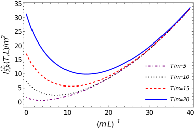
Figure 1: Panel (a): The variation of the renormalized two-point function with $T$ and $L$. Panel (b), the same but for fixed values of the temperature. We have assumed $\mu=m$ for illustration.

As an immediate consequence of the behavior of $I^{(1),{\rm DBC}}_{2,{\rm R}}$ as a function of $T$ and $L$ will be the possibility of having behavior analogous to reentrant phase transitions as we will demonstrate in Sec. V.

IV Renormalized masses and couplings and resummation procedure

Let us discuss in this section both the dependence of the renormalized masses and couplings with the scale and also the resummation procedure we have adopted to analyze the phase transition patterns at both finite temperature and size.

IV.1 Dependence of the masses and couplings with the renormalization scale

Before presenting our results, let us discuss the dependence of the masses and coupling in our model with the renormalization scale $\mu$.

As already mentioned in the previous section, it is enough for us here to work the renormalization of the system in the bulk. Working at the one-loop level, the renormalized masses and coupling constants can then be readily computed (see, for instance Ref. Kleinert:2001hn ) and they are given by

$$m_{\phi}^{2}(\mu) = \bar{m}_{\phi}^{2}+\frac{\bar{\lambda}_{\phi}}{2}\left(\frac{N_{\phi}+2}{3}\right)\frac{\bar{m}_{\phi}^{2}}{16\pi^{2}}\left[-1+\ln\left(\frac{\bar{m}_{\phi}^{2}}{\mu^{2}}\right)\right]$$ (36)

$$+ \frac{\bar{\lambda}}{2}N_{\chi}\frac{\bar{m}_{\chi}^{2}}{16\pi^{2}}\left[-1+\ln\left(\frac{\bar{m}_{\chi}^{2}}{\mu^{2}}\right)\right],$$

$$m_{\chi}^{2}(\mu) = \bar{m}_{\chi}^{2}+\frac{\bar{\lambda}_{\chi}}{2}\left(\frac{N_{\chi}+2}{3}\right)\frac{\bar{m}_{\chi}^{2}}{16\pi^{2}}\left[-1+\ln\left(\frac{\bar{m}_{\chi}^{2}}{\mu^{2}}\right)\right]$$ (37)

$$+ \frac{\bar{\lambda}}{2}N_{\phi}\frac{\bar{m}_{\phi}^{2}}{16\pi^{2}}\left[-1+\ln\left(\frac{\bar{m}_{\phi}^{2}}{\mu^{2}}\right)\right],$$

$$\lambda_{\phi}(\mu) = \bar{\lambda}_{\phi}+\frac{(N_{\phi}+8)\bar{\lambda}_{\phi}^{2}}{6(4\pi)^{2}}\ln\left(\frac{\bar{m}_{\phi}^{2}}{\mu^{2}}\right)$$ (38)

$$+ \frac{3N_{\chi}\bar{\lambda}^{2}}{2}\ln\left(\frac{\bar{m}_{\chi}^{2}}{\mu^{2}}\right),$$

$$\lambda_{\chi}(\mu) = \bar{\lambda}_{\chi}+\frac{(N_{\chi}+8)\bar{\lambda}_{\chi}^{2}}{6(4\pi)^{2}}\ln\left(\frac{\bar{m}_{\chi}^{2}}{\mu^{2}}\right)$$ (39)

$$+ \frac{3N_{\phi}\bar{\lambda}^{2}}{2}\ln\left(\frac{\bar{m}_{\phi}^{2}}{\mu^{2}}\right),$$

$$\lambda(\mu) = \bar{\lambda}+2\bar{\lambda}^{2}\frac{1}{\bar{m}_{\phi}^{2}-\bar{m}_{\chi}^{2}}\left\{\frac{\bar{m}_{\phi}^{2}}{16\pi^{2}}\left[-1+\ln\left(\frac{\bar{m}_{\phi}^{2}}{\mu^{2}}\right)\right]\right.$$ (40)

$$- \left.\frac{\bar{m}_{\chi}^{2}}{16\pi^{2}}\left[-1+\ln\left(\frac{\bar{m}_{\chi}^{2}}{\mu^{2}}\right)\right]\right\}$$

$$+ \frac{(N_{\phi}+2)\bar{\lambda}\bar{\lambda}_{\phi}}{6(4\pi)^{2}}\ln\left(\frac{\bar{m}_{\phi}^{2}}{\mu^{2}}\right)$$

$$+ \frac{(N_{\chi}+2)\bar{\lambda}\bar{\lambda}_{\chi}}{6(4\pi)^{2}}\ln\left(\frac{\bar{m}_{\chi}^{2}}{\mu^{2}}\right),$$

with the above equations depending on the renormalization scale $\mu$ through the $\overline{\rm MS}$ parameters of the renormalized Lagrangian. Note that in the above equations we are expressing all bare quantities (which does not depend on the scale $\mu$), and that appears on the right-hand side of the equations, as a barred quantity. The renormalized parameters, on the other hand, are all dependent on the scale $\mu$.

Finally, note that the above equations apply to the symmetry restored case where $\bar{m}_{i}^{2}>0$. In the symmetry broken case, the procedure is well-known (see, for instance Refs. Nishijima:1979yx ; Taylor:1983xu ; Brown:1988yj for details of the corresponding renormalization group (RG) procedure): the fields are shifted around the true mininum, leading to bare and renormalized masses, when in the vacuum, replaced by $\bar{m}_{i}^{2}\to 2|\bar{m}_{i}^{2}|$ and $m_{i}^{2}\to 2|m_{i}^{2}|$, respectively.

The renormalization scale dependence on both masses and couplings are given in terms of their respective RG expressions, given in terms of the RG functions $\beta$ and $\gamma_{m}$ given, respectively, by Kleinert:2001hn

$$\beta_{i}=\mu\frac{\partial\lambda_{i}}{\partial\mu},$$ (41)

and

$$\gamma_{m_{i}}=\mu\frac{\partial\ln m_{i}}{\partial\mu},$$ (42)

which, for our respective masses and couplings and at one-loop ($\hbar$) order, give

$$\gamma_{m_{\phi}}=\frac{1}{2m_{\phi}^{2}(\mu)(4\pi)^{2}} \left[\lambda_{\phi}(\mu)\frac{(N_{\phi}+2)}{3}m_{\phi}^{2}(\mu)\right.$$ (43)

$$+\left.\lambda(\mu)N_{\chi}m_{\chi}^{2}(\mu)\frac{}{}\right],$$

$$\gamma_{m_{\chi}}=\frac{1}{2m_{\chi}^{2}(\mu)(4\pi)^{2}} \left[\lambda_{\chi}(\mu)\frac{(N_{\chi}+2)}{3}m_{\chi}^{2}(\mu)\right.$$ (44)

$$+\left.\lambda(\mu)N_{\phi}m_{\phi}^{2}(\mu)\right],$$

$$\beta_{\lambda_{\phi}}=\frac{(N_{\phi}+8)}{3}\frac{\lambda_{\phi}^{2}(\mu)}{(4\pi)^{2}}+3N_{\chi}\frac{\lambda^{2}(\mu)}{(4\pi)^{2}},$$ (45)

$$\beta_{\lambda_{\chi}}=\frac{(N_{\chi}+8)}{3}\frac{\lambda_{\chi}^{2}(\mu)}{(4\pi)^{2}}+3N_{\phi}\frac{\lambda^{2}(\mu)}{(4\pi)^{2}},$$ (46)

$$\beta_{\lambda} = 4\frac{\lambda^{2}(\mu)}{(4\pi)^{2}}+\frac{(N_{\phi}+2)}{3}\frac{\lambda(\mu)\lambda_{\phi}(\mu)}{(4\pi)^{2}}$$ (47)

$$+ \frac{(N_{\chi}+2)}{3}\frac{\lambda(\mu)\lambda_{\chi}(\mu)}{(4\pi)^{2}}.$$

Equations (43)-(47) form a coupled set of flow equations determining how the masses and couplings change under different renormalization scales. In particular, we can also see from, e.g., Eqs. (45), (46) and (47), that their solution is also equivalent to solving the coupled set of linear equations,

$$\lambda_{\phi}(\mu) = \lambda_{\phi}(\mu_{0})+\frac{1}{(4\pi)^{2}}\ln\left(\frac{\mu}{\mu_{0}}\right)$$

$$\times \left[\frac{(N_{\phi}+8)}{3}\lambda_{\phi}(\mu_{0})\lambda_{\phi}(\mu)+3N_{\chi}\lambda(\mu_{0})\lambda(\mu)\right],$$

$$\lambda_{\chi}(\mu) = \lambda_{\chi}(\mu_{0})+\frac{1}{(4\pi)^{2}}\ln\left(\frac{\mu}{\mu_{0}}\right)$$

$$\times \left[\frac{(N_{\chi}+8)}{3}\lambda_{\chi}(\mu_{0})\lambda_{\chi}(\mu)+3N_{\phi}\lambda(\mu_{0})\lambda(\mu)\right],$$

$$\lambda(\mu) = \lambda(\mu_{0})+\frac{\lambda(\mu_{0})}{(4\pi)^{2}}\ln\left(\frac{\mu}{\mu_{0}}\right)$$ (50)

$$\times \left[\frac{1}{2}\left(\frac{N_{\phi}+2}{3}\right)\lambda_{\phi}(\mu)+\frac{1}{2}\left(\frac{N_{\chi}+2}{3}\right)\lambda_{\chi}(\mu)\right]$$

$$+ \frac{\lambda(\mu)}{(4\pi)^{2}}\ln\left(\frac{\mu}{\mu_{0}}\right)$$

$$\times \left[\frac{1}{2}\left(\frac{N_{\phi}+2}{3}\right)\lambda_{\phi}(\mu_{0})+\frac{1}{2}\left(\frac{N_{\chi}+2}{3}\right)\lambda_{\chi}(\mu_{0})\right]$$

$$+ \frac{1}{4\pi^{2}}\ln\left(\frac{\mu}{\mu_{0}}\right)\lambda(\mu_{0})\lambda(\mu),$$

which also make apparent how the renormalized couplings are related through a change of the scale from, e.g., $\mu_{0}$ to $\mu$. The results obtained from the flow equations given above give the standard way of nonperturbatively resumming through the RG equations the leading order corrections (in this case the leading log-dependent corrections) to the coupling constants. These equations also show that the couplings evolve with the scale in a logarithmic way. Suitable choices of the scale can minimize these logarithmic contributions. It is common in the literature in general that at high temperatures to take the scale proportional to the temperature, $\mu\sim T$. In particular, a suitable choice of scale has been shown to be given by Drummond:1997cw $\mu=2\pi T$.

The typical strategy is followed: for example, in the hard-thermal loop analysis of the thermodynamics (see, for example, Ref. Andersen:2004fp ), we can express all physical quantities in terms of the renormalized, scale-dependent, parameters. Working similarly here, this means, for instance, the set of renormalized parameters are given at the reference scale $\mu_{0}$. By a change of the scale (e.g., with the temperature, or, in our present problem can also be with $L$), the new set of renormalized parameters related to the original ones fixed at the reference scale $\mu_{0}$ are then obtained by solving the coupled flow equations, Eqs. (43)-(47), for the new value $\mu$. The bare parameters are then finally determined by inverting the set of equations (36)-(40), getting $\bar{m}_{\phi}(m_{\phi},m_{\chi},\lambda_{\phi},\lambda_{\chi},\lambda)$, etc.

At finite sizes, we also see from the equations derived earlier, Eqs. (28) and (29), that those equations suggest that a more suitable scale might be $\mu\sim 1/L$ when $TL<1/2$. In practice, in all of our numerical analysis, we will adopt for the reference scale $\mu_{0}=2\pi T$ or $\mu_{0}=2\pi/L$, depending whether the temperature or the (inverse of the) length size dominates the loop integrals. As typically adopted in the literature to check the variation of the results with the scale $\mu$, we will then vary $\mu$ in a range $\alpha=\mu/\mu_{0}=[1/2,2]$. Either way, the logarithmic dependence on the scale will imply that all of our results will be weakly dependent on the particular choice of $\mu$, provided that the couplings, $T$ and $1/L$ are not too large. In the parameters we will be working with our examples in Sec. V, this will always be the case.

IV.2 The bubble (ring) resummed gap equations for the masses and field expectation values

We want to investigate the full phase structure for the multiple field system. However, it is well known that PT breaks down at high temperatures and, in particular close to critical points Bellac:2011kqa . Here, we go beyond the perturbation theory by using the bubble (or ring) dressed method for finite-temperature scalar fields Espinosa:1992gq . In the bubble resummation procedure, the one-loop terms with the temperature and finite-size effects are self-consistently resummed by using the gap equations for the masses, which is similar as previously considered in ISB/SNR earlier studies Roos:1995vm ; Pinto:2005ey ; Pinto:2006cb ; Phat:2007zz . In this case, this is equivalent of solving the coupled system of gap equations for the renormalized masses,

$$M_{\phi}^{2} = \bar{m}_{\phi}^{2}+\frac{\bar{\lambda}_{\phi}}{2}\left(\frac{N_{\phi}+2}{3}\right)I^{(1)}_{2,R}(M_{\phi},T,L)$$ (51)

$$+ \frac{\bar{\lambda}}{2}N_{\chi}I^{(1)}_{2,R}(M_{\chi},T,L),$$

$$M_{\chi}^{2} = \bar{m}_{\chi}^{2}+\frac{\bar{\lambda}_{\chi}}{2}\left(\frac{N_{\chi}+2}{3}\right)I^{(1)}_{2,R}(M_{\chi},T,L)$$ (52)

$$+ \frac{\bar{\lambda}}{2}N_{\phi}I^{(1)}_{2,R}(M_{\phi},T,L),$$

where the renormalized one-loop function $I^{(1)}_{2,R}$ is given by Eq. (19) with the divergence subtracted.

The fields are shifted around their expectation values, $\phi\to\bar{\phi}+\phi^{\prime}$ and $\chi\to\bar{\chi}+\chi^{\prime}$, where $\bar{\phi}\equiv\langle\phi\rangle$ and $\bar{\chi}\equiv\langle\chi\rangle$, while $\langle\phi^{\prime}\rangle=0$ and $\langle\chi^{\prime}\rangle=0$. The expectation values for the fields are then defined through their respective coupled tadpole equations, given by, respectively, in terms of the one-particle irreducible (1PI) one-point functions $\Gamma^{(1)}_{\phi}\equiv 0$ and $\Gamma^{(1)}_{\chi}\equiv 0$. At the one-loop level and resummed bubble approximation, we have that

$$\Gamma^{(1)}_{\phi} = -\bar{m}_{\phi}^{2}\bar{\phi}-\frac{\bar{\lambda}_{\phi}}{6}\bar{\phi}^{3}-\frac{\bar{\lambda}}{2}\bar{\phi}\bar{\chi}^{2}$$ (53)

$$- \frac{(N_{\phi}+2)}{6}\bar{\lambda}_{\phi}\bar{\phi}I^{(1)}_{2,R}(\tilde{\Omega}_{\phi},T,L)$$

$$- \frac{N_{\chi}}{2}\bar{\lambda}\bar{\phi}I^{(1)}_{2,R}(\tilde{\Omega}_{\chi},T,L)\equiv 0,$$

$$\Gamma^{(1)}_{\chi} = -\bar{m}_{\chi}^{2}\bar{\chi}-\frac{\bar{\lambda}_{\chi}}{6}\bar{\chi}^{3}-\frac{\bar{\lambda}}{2}\bar{\phi}^{2}\bar{\chi}$$ (54)

$$- \frac{(N_{\chi}+2)}{6}\bar{\lambda}_{\chi}\bar{\chi}I^{(1)}_{2,R}(\tilde{\Omega}_{\chi},T,L)$$

$$- \frac{N_{\phi}}{2}\bar{\lambda}\bar{\chi}I^{(1)}_{2,R}(\tilde{\Omega}_{\phi},T,L)\equiv 0,$$

where $\tilde{\Omega}_{\phi}$ and $\tilde{\Omega}_{\chi}$ are defined, respectively, by

$$\tilde{\Omega}_{\phi}^{2} = M_{\phi}^{2}+\frac{\bar{\lambda}_{\phi}}{2}\bar{\phi}^{2}+\frac{\bar{\lambda}}{2}\bar{\chi}^{2},$$ (55)

$$\tilde{\Omega}_{\chi}^{2} = M_{\chi}^{2}+\frac{\bar{\lambda}_{\chi}}{2}\bar{\chi}^{2}+\frac{\bar{\lambda}}{2}\bar{\phi}^{2}.$$ (56)

We now have the complete set of necessary equations to analyze the phase structure of the coupled two-scalar field system.

V Results

Let us now consider the combined effects of temperature and finite size in the phase transition patterns in the two-scalar field model. But before studying the coupled two-field system, it is instructive to first analyze the case of only one field, e.g., $\phi$, which can be easily obtained by setting the intercoupling $\lambda$ to zero in the equations defined in the previous section.

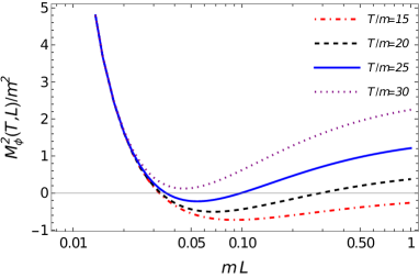
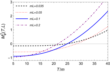
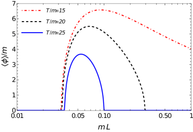
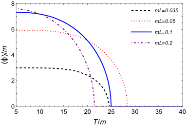
Figure 2: The effective gap mass squared for $\phi$ and the expectation value $\langle\phi\rangle$ in the one-field case ($\lambda=0$) in the case of a symmetry breaking tree-level potential as a function of the length $L$ for fixed values of temperature (panels a and c) and as a function of the temperature $T$ for fixed values of length $L$ (panels b and d). The renormalization scale is here fixed at the reference scale, $\mu=\mu_{0}$ (see Sec. IV.1), the renormalized coupling constant is $\lambda_{\phi}(\mu_{0})=0.1$, we have also considered $N_{\phi}=1$ and all dimensional quantities are in units of the renormalized mass $m\equiv m(\mu_{0})$.

V.1 The one-scalar field case

Setting the tree-level mass square term in the potential as negative, i.e., $\bar{m}_{\phi}^{2}=-|\bar{m}_{\phi}|^{2}\equiv-m^{2}$, in Fig. 2 we show the effective mass $M_{\phi}(T,L)$ and the field expectation value $\langle\phi\rangle$ in the DBC as a function of $L$ for fixed temperature values [panels (a) and (c)] and as a function of the temperature for fixed values of $L$ [panels (b) and (d)].

From Figs. 2(a) and 2(c) we can see that the effect of the compact dimension allows the system to have a double critical point, where the symmetry can get broken in between two values of critical length $L_{c}$. This is a reentrant phase transition, which might be of interest in condensed matter systems Pinto:2005ey ; Ramos:2006er ; Pinto:2006cb ; Linhares:2012vr . These type of transitions are also of interest for understanding, for example, phase transitions in superconducting films, as studied previously in Ref. Linhares:2006my , which considered finite-size effects in a Ginzburg–Landau model with periodic boundary conditions. The same trend of transitions also is seen to happen here in the context of DBC. In Figs. 2(b) and 2(d) the SR behavior as a function of temperature is shown for some fixed values of length $L$. Here we note that although there seems to be no multiple critical points in the temperature (e.g., the appearance of two critical values of temperature), it shows instead that for small values of $L$ the critical temperature tends to grow as $L$ increases, but then $T_{c}$ starts to decrease beyond some value of $L$. Note that the phase transition points agree between the results shown for either the effective gap mass or the field expectation value, as they should. We can also notice from the results displayed in the panels of Fig. 2 that the transition is always continuous, which characterize a second-order phase transitions for all the cases displayed in Fig. 2.

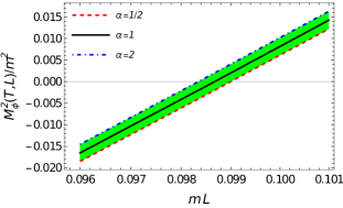
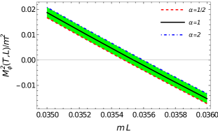
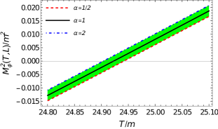
Figure 3: A detailed view of the variation of the critical points with respect to changes in the renormalization scale around the reference value $\mu_{0}$. The region around the two critical points in the length $L$ shown in Fig. 2(a) for $T/m(\mu_{0})=25$ are here shown in the panels (a) and (b). Panel (c) shows the region around the critical point in the temperature for the case with $m(\mu_{0})L=0.1$ shown in Fig. 2(b).

At this point, it becomes useful to analyze the dependence of any of these results with the variation of the scale. Let us remainder that a sensitive of the results with the renormalization scale $\mu$ can also be seen as an indicator of the reliability of the approximation method which is being used in our study, i.e., the bubble resummation scheme explained in Sec. IV.2. For instance, the effective mass here is directly related to the 1PI two-point function at zero momentum, $\Gamma^{(2)}_{i}(0,0)\equiv-M_{i}^{2}$ and $\Gamma^{(2)}_{i}$ must satisfy the RG equation Peskin:1995ev ,

$$\mu\frac{d\Gamma^{(2)}_{i}}{d\mu}=0.$$ (57)

Of course, since we cannot evaluate $\Gamma^{(2)}_{i}$ to arbitrary precision, the level of sensitive of it on the renormalization scale gives us an indication of the level of accuracy of the method used in its derivation.

As already explained at the end of Sec. IV.1, we follow the standard procedure usually adopted in many of the studies in the context of the hard thermal loop and vary $\mu$ with respect to the reference scale by a factor of two, $\mu/\mu_{0}\equiv\alpha=[1/2,2]$. This typically gives a good indicator of how relevant thermodynamical quantities (like the pressure) are sensitive to the scale Andersen:2004fp . Taking for instance the example shown in Fig. 2 in the cases of $T/m(\mu_{0})=25$ and $m(\mu_{0})L=0.1$ (solid line in Figs. 2(a) and  2(b), respectively), the effect of changing the scale is very small. This is illustrated in Fig 3 by zooming in around each of the critical points shown in there. Our results show that the considered variation of the renormalization scale leads to a change in the critical points by around the one percent level and smaller. This is in a sense consistent with the fact that we are considering not large couplings neither is the temperature is too large to cause a significant change here (recalling from the flow equations that variations with the scale are logarithmic).

Figure 3 shows the behavior for the effective mass $M_{\phi}$ close to the transition points in the temperature and length. The same can be done also for the field expectation value $\langle\phi\rangle$ shown in Figs. 2(c) and  2(d). Let us recall that the inverse of the effective mass is equivalent to the correlation length of the field, $\xi_{\phi}=1/M_{\phi}$, while $\langle\phi\rangle$ makes the role of the order parameter for the phase transition, much the same way as the correlation length and magnetization, respectively, for an Ising system in three spatial dimensions in the context of statistical physics Parisi:1988nd . The way these quantities approach the critical point are specified by the critical exponents $\nu$ and $\beta$, which can be defined as

$$\nu=\lim_{\tau\to 0}\frac{\ln|M_{\phi}(\tau)|}{\ln|\tau|},$$ (58)

$$\beta=\lim_{\tau\to 0}\frac{\ln\langle\phi\rangle(\tau)}{\ln|\tau|},$$ (59)

where, in the usual prescription, $\tau$ denotes the reduced temperature, $\tau=(T-T_{c})/T_{c}$ and $T_{c}$ is the critical temperature. In the present problem, the critical point can be approached by varying either the temperature or the length $L$. Hence, we can define $\tau$ with respect to either $T$ or $L$, according to the equivalence between $T$ and $1/L$ already discussed at the end of Sec. III, and make estimates concerning the critical exponents $\nu$ and $\beta$. Already from Fig. 3 we can see that the effective mass square always approaches the critical point in a linear way. Since we expect that $M_{\phi}^{2}\propto|\tau|^{2\nu}$ as $\tau\to 0$, hence, $\nu=1/2$. The same can be studied for how the expectation value of the field approaches the critical points. Taking sufficiently small values for $\tau$, we verify that here too we get $\beta=1/2$. These are the mean-field critical exponents and which are expected for the level of approximation we are presently considering. Deviations from the mean-field values are only expected to happen when the full two-loop order terms are also resummed and to approach the expected critical exponents for this problem can only be achieved through a three-loop and higher-order resummation scheme (see, e.g., Ref. Kleinert:2001hn for some examples).

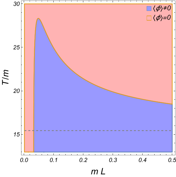
Figure 4: The phase diagram for the one-field case in the plane $(L,T)$ for the case of the same parameters used in Fig. 2. The horizontal dashed line indicates the critical temperature in the case of $L\to\infty$, $T_{c}(L\to\infty)/m\simeq 15.5$.

Finally, for illustration, the different transition behaviors displayed in Fig. 2 are shown in the phase diagram depicted in Fig. 4, where the regions of symmetry breaking, $\langle\phi\rangle\neq 0$, and symmetry restored, $\langle\phi\rangle=0$, are shown in the plane $(L,T)$.

The variation of the renormalization scale in the same range considered in Fig. 3 only leads to very small changes (at most at the one percent level) in the critical curve shown in Fig. 4 and, therefore, it is not shown explicitly. The phase diagram depicted in Fig. 4 shows that the critical temperature fast increases when $L$ is increased when starting from very small values ($mL\gtrsim 0.03$), reaches a maximum at $mL\simeq 0.05$ and then decreases towards large $L$. The horizontal dashed line indicates the critical temperature in the case of the absence of finite-size effects ($L\to\infty$), whose value for the parameters used in Fig. 4 is found to be $T_{c}(L\to\infty)/m\simeq 15.5$. The behavior analogous to reentrant phase transitions as a function of $L$ are clearly visible when taking constant temperature values and that happens with temperatures in the range $15.5\lesssim T/m\lesssim 28$.

The phase structure behavior displayed in Fig. 4 is easy to understand when we look at the temperature and size dependence of the loop integral $I_{2}^{(1)}$ discussed at the end of Sec. III. The reentrant behavior is directly related to the fact that the loop integral $I_{2}^{(1)}$ displays a minimum for ranges of values for $T$ and $L$ as shown in Fig. 1. For fixed $L$ and increasing $T$, as $I_{2}^{(1)}\propto T^{2}$, eventually SR is realized. Finally, when $L$ is decreased with fixed $T$, again we see that since now $I_{2}^{(1)}\propto 1/L^{2}$, then the symmetry will also be restored for sufficiently small values of $L$, as it is explicitly seen in Fig. 4.

V.2 The two-scalar field case

Let us now study the multiscalar field case, i.e., including both $\phi$ and $\chi$ with a nonvanishing intercoupling $\lambda$ between them. We are mainly interested in exploring a parameter space where the usual SR can happen at high temperatures along a given field direction, while the other field experiences ISB. Let us first recall that from the PT estimates from Sec. II, considering a negative intercoupling $\lambda$, when Eq. (4) is observed, but still satisfying the boundness condition Eq. (2), we expected an ISB phase transition in the i-field direction, when $m_{i}^{2}>0$, or, equivalently, a SNR, when $m_{i}^{2}<0$. According to the previous discussions, these phase transition patterns are expected at either at high temperatures (at fixed $L$), or, likewise, at small values of the length, $L\ll 1/m,1/T$ (at fixed $T$). By focus on the ISB case, let us investigate first the parameter space that leads to this phase transition pattern.

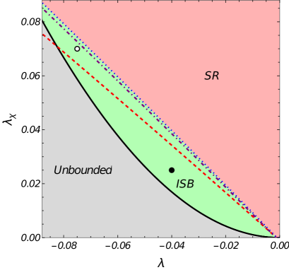
Figure 5: The parameter space able to lead to inverse symmetry breaking in the case of a fixed value of $\lambda_{\phi}=0.8$. The black and white (open) dots in the figure indicate, respectively, the locations for the parameter sets I and II used in our numerical studies. The solid line delimits the region satisfying the boundness of the potential. The dotted and dashed lined delimits the separation between the SR and ISB phases in the cases of PT and the nonperturbative bubble resummation procedure in the case of the bulk ($L\to\infty$) and for a sufficiently high temperature. The dash-dotted line in between them indicates a boundary set when using a finite value for $L$, $mL=0.075$.

Without loss of generality, we can consider, for example, the two sets of renormalized couplings: Set I: $\lambda_{\phi}=0.8,\,\lambda_{\chi}=0.025$ and $\lambda=-0.04$; and Set II: $\lambda_{\phi}=0.8,\,\lambda_{\chi}=0.07$ and $\lambda=-0.075$ , along also with the initial choice $N_{\phi}=N_{\chi}=1$. Both sets of couplings satisfy Eq. (2). Then, with the perturbation equations in the high-temperature approximation, e.g., Eq. (3), they predict an ISB phase transition along the direction of the $\chi$ field whenever $m_{\chi}^{2}>0$. On the other hand, for $m_{\chi}^{2}<0$, SNR should manifest, in which case the $\chi$-field expectation value should always remain as nonvanishing, $\langle\chi\rangle\neq 0$. The symmetry behavior along the $\phi$ field direction depends only on the sign of its mass square term entering in the Lagrangian density. For $m_{\phi}^{2}>0$, it (in the $\phi$ field direction) remains in a symmetry restored phase, $\langle\phi\rangle=0$, while considering initially (at $T=0$) a symmetry broken (SB) phase along the $\phi$ field direction, i.e., $m_{\phi}^{2}<0$, the usual symmetry restoration at high temperatures is expected. Of course, had we chosen different assignments for the couplings, the roles of the $\phi$ and $\chi$ fields are expected to be reversed under the phenomena of SB/SR and ISB/SNR. For definiteness, in the analysis that follow, we will consider that $\phi$ suffers the usual SR at high temperatures, while $\chi$ should experience ISB, i.e., we choose the mass renormalized parameters such that $m_{\phi}^{2}<0$ and $m_{\chi}^{2}>0$ and under the above given choice of representative values for the two sets of coupling constants. Of course, other combinations of parameters could be used but the results could be similarly interpreted.

It is useful to show the two sets of couplings that we are considering here in a given plane in the coupling constants parameter space. With $\lambda_{\phi}=0.8$. in Fig. 5, we present the parameter available for ISB. The location of the sets I and II are represented by the black dot and white (open) points, respectively. The region in between the solid and dotted lines is the region for ISB predicted by PT according to Eq. (4) and when $L\to\infty$. The region for ISB according to the nonperturbative results coming from the solution of the gap equations is, however, delimited by the solid and dashed lines (also when $L\to\infty$). Note that there is reduction of the parameter region available for ISB when compared to PT. The dash-dotted line delimits the region for ISB for the case of finite $L$, which is taken as $L=0.075/m$ in the example shown in Fig. 5. Note that the finite-size effect is to enlarge the region for ISB when compared to the result at $L\to\infty$.

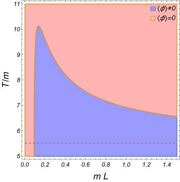
(a) Parameter set I

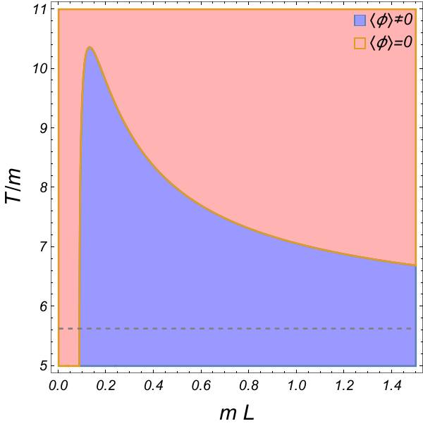
(b) Parameter set II

Figure 6: The phase diagram for $\phi$ in the coupled field case in the plane $(L,T)$. The horizontal dashed line indicates the critical temperature in the case of $L\to\infty$, $T_{c}(L\to\infty)/m\simeq 5.52$ (set I) and $T_{c}(L\to\infty)/m\simeq 5.63$ (set II).

In both parameter sets I and II we expect that the field $\phi$ will experience the usual SR as the temperature increases. Also, as in the one-field case studied in the previous subsection, as we decrease $L$, SR is also expected. This is explicitly illustrated in Fig. 6, where the transition pattern for $\phi$ in both sets of parameters is shown. Figure 6 shows again the characteristic reentrant (double transition point) like behavior as the compactification size $L$ is changed and a maximum critical temperature that can be reached when $L$ changes. Note that in the results shown in Fig. 6 and the next ones, we have verified explicitly that the change in the scale $\mu$ only leads to small corrections, just like in the one-field case, and causes no change in our conclusions regarding the phase transition patterns reported here. Thus, all the following results are presented only at the reference scale $\mu_{0}$.

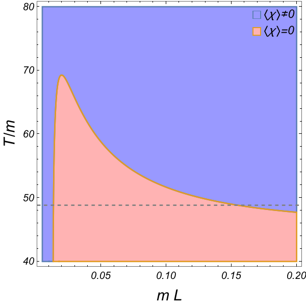
(a) Parameter set I

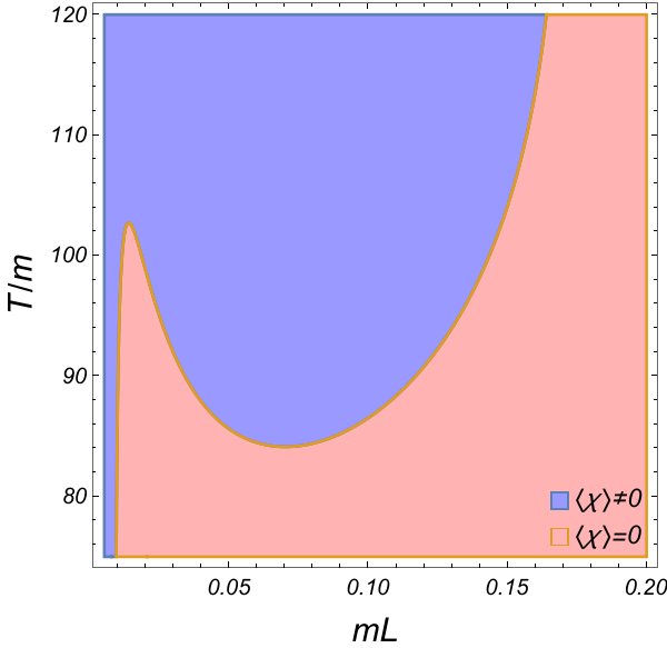
(b) Parameter set II

Figure 7: The phase diagram for $\chi$ in the coupled field case in the plane $(L,T)$. The horizontal dashed line in the case of panel (a) indicates the critical temperature in the case of $L\to\infty$, $T_{c}(L\to\infty)/m\simeq 48.8$.

The situation becomes more interesting when we now analyze the transition pattern for the field $\psi$. In the parameter set I we expect the field $\psi$ to display ISB just like in the case of the bulk case ($L\to\infty$). This is indeed the case as shown in Fig. 7(a) when $L$ is increased. However, as expected, ISB also manifests in the small $L$ region, for the same reason as discussed for the transition in the $\phi$ direction (though now instead of SR, we have ISB) and it is again due to the behavior displayed by the loop function in terms of $L$ and $T$. Note that now, we have a reentrant transition to a symmetry restored phase in between the two extremes. However, for the parameter set II, which resides in between the dashed line ($L\to\infty$) and the finite $L$ region shown in Fig. 5, we do not expect ISB to persist for large values of $L$, as the dash-dotted line moves towards the dashed line and the point will reside in the SR phase. Thus, here, ISB is truly only a consequence of the finite-size effect as illustrated in Fig. 7(b).

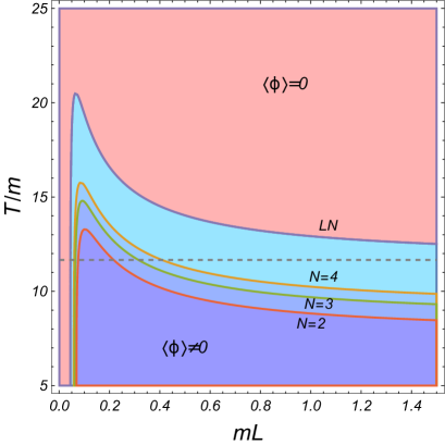
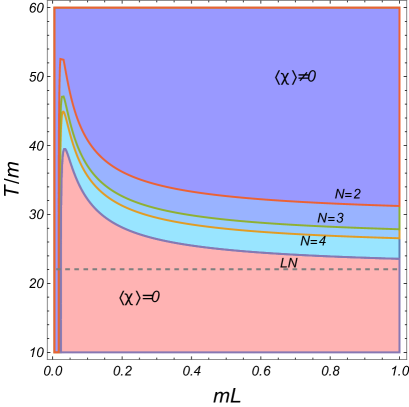
Figure 8: The phase diagram for $\phi$ (panel a) and for $\chi$ (panel b) in the coupled field case in the plane $(L,T)$ using the LN approach. The parameters chosen are the same as the set II considered in Figs. 6 and 7, $m_{\phi}^{2}=-m_{\chi}^{2}=m^{2}>0$, $\lambda_{\phi}=0.8,\,\lambda_{\chi}=0.07$ and $\lambda=-0.075$. The horizontal dashed line indicates the critical temperature in the LN approximation and in the bulk case ($L\to\infty$), $T_{c,\phi}^{\rm LN}(L\to\infty)/m\simeq 11.7$ and $T_{c,\chi}^{\rm LN}(L\to\infty)/m\simeq 22$.

VI Finite $N$ effects and comparison with the large-$N$ approximation

So far, in the previous section we have restricted to cases where $N_{\phi}=N_{\chi}=1$, i.e., in the context of a two-field model with symmetry $Z_{2}\times Z_{2}$. Let us now investigate how those results might get affected by finite $N$ effects. It is useful in this context to compare the finite $N$ results with the ones derived in the context of the large-$N$ approximation.

In the large-$N$ (LN) approximation (for a review, see, e.g., Ref. Moshe:2003xn ) both coupling constants and fields are normalized by $N$, such that, for instance, $\lambda_{i}\to\lambda_{i}/N_{i}$, $\lambda\to\lambda/\sqrt{N_{\phi}N_{\chi}}$, $\phi\to\sqrt{N_{\phi}}\phi$ and $\chi\to\sqrt{N_{\chi}}\chi$, while the rescaled coupling are kept fixed as $N_{i}\to\infty$. Without loss of generality, we will consider $N_{\phi}=N_{\chi}\equiv N$. Note that in the LN approximation, the simple one-loop expressions, e.g., Eqs. (22) and (23), become exact, since higher order terms become suppressed by factors of $1/N_{i}$. Next, we will compare the LN approximation result for the phase diagram in the plane $(L,T)$ for $\phi$ and $\chi$ with the corresponding finite $N$ ones constructed in this approach. In Fig. 8(a) we show the result for the phase diagram for $\phi$, while in Fig. 8(b) it is shown the result for $\chi$. We have used the values $N=2$, $N=3$ and $N=4$ for comparison, which can be motivated by, e.g., coupled complex scalar fields with $O(2)\times O(2)$ symmetry, coupled Heisenberg type of models with $O(3)\times O(3)$ symmetry, or a coupled linear $\sigma$-model with $O(4)\times O(4)$ symmetry, respectively. The set of parameters considered was set II, which was used in previous subsection. We note that for the large-$N$ case, as also for the finite $N$ examples shown in Fig. 8, the point represented by the parameter set II moves to the ISB inner region shown in Fig. 5. Hence, as oppositely seen in Fig. 7 in the case of $N_{\phi}=N_{\chi}=1$, here ISB persists even at larger values of $L$. We also note from the results shown in Figs. 8 that in the LN approximation we still observe reentrant phases with double critical values for $L$ in both the $\phi$ and $\chi$ directions.

VII Conclusions

In this work we have investigated the possible phase transitions patterns in a two-field multicomponent scalar model with symmetry $O(N_{\phi})\times O(N_{\chi})$ when both thermal and finite-size effects are present. While in the bulk (in the absence of space boundaries) phenomena like ISB have shown to be present at high temperatures, when the intercoupling between the fields is negative, the phase transition patterns when finite-size effects are present become more involved. The finite-size effects allow the system to display behavior analogous to reentrant symmetry breaking (which can happen in between two phases of symmetry restoration) and vice versa, where symmetry restoration can happen in between two phases of symmetry breaking. These type of phenomena can happen for both fields depending on the choice of parameters and they are a consequence of the behavior of the one-loop integral as a function of $T$ and $L$, which presents a minimum depending on the choice of temperature and length. In this work we have analyzed these phase transition phenomena with the use of the bubble (or ring) resummed gap equations for both the effective masses for the fields and for their expectation values, $\langle\phi\rangle$ and $\langle\chi\rangle$. The results were also compared with the large-$N$ approximation. The behavior analogous to reentrant symmetry breaking for the fields was shown to be present in both cases.

We have considered in this paper the Dirichlet boundary condition for the space compactification in a slab geometry in the three-dimensional space, $\mathbb{R}^{2}\times[0,L]$. The Dirichlet boundary condition is a well-motivated condition for different physical systems as has been argued in the recent literature. For practical purposes, it is also computationally convenient since there are no zero modes when working with the discrete frequencies and, consequently, direct simple equations in the limit of large temperature can be derived. We have obtained the expressions for the two-point one-loop self-energy correction contributing to the effective masses and we have also made use of the renormalized parameters (masses and coupling constants). We have shown that typical variations of the scale around a reference value do not change in any significant way the transition patterns describe and found in this work, with the variations with the scale remaining small. This fact can be used as an additional argument concerning the reliability of the approximation used. Our results can, in principle, also be extended to higher loops, which would allow eventually to explore regions of larger couplings than the ones we have considered here.

Other types of geometries can also be considered as future developments of this work. But still, the simpler slab geometry here considered can be of interest in practical physical applications, most notably, like in condensed matter problems where, for example, the thickness of thin films are important material1 ; material2 ; material3 ; material4 ; material5 . With the advent of even more miniaturized electronic devices, it is extremely relevant to analyze how the size and interface effects change the properties and performances of nanomaterials. In particular, similar phase transition behaviors as a function of the thickness that resembles the ones we have seen here, have also been observed in different materials. For instance, a rapid grow of the critical temperature with the thickness and then a smooth decrease of $T_{c}$, as it appears in Figs. 2, 6 and 8, for example, have been experimentally measured in different materials displaying superconductivity transitions (see, e.g., Ref. material6 ). In this context, even though we have here considered a relativistic type of model, our results can still be of interest in applications in the condensed matter context. For instance, excitons type of systems exhibit a relativistic dispersion relation Lopes:2019mjc and, furthermore, are effectively modeled as a multifield scalar model for which our results can be directly applied to. Our results can also be of interest for high-energy relativistic systems. Relativistic type of systems typically modeled by multifield scalar models with both inter and intracouplings include for example those in the context of color-flavor superconductivity Alford:2007qa ; Andersen:2008tn ; Silva:2023jrk , which the study of the effect of space compactifications can be of relevance. In addition, other applications are also possible, like, for example, to infer possible finite-size effects in the transition from a quark-gluon plasma to hadronic matter in the case of the fireball formed in the collision of heavy ions. The pancake like shape of the formed plasma (for a review, see, e.g.. Ref. Nguyen:2020zux ) suggest that at the central region our slablike geometry might be relevant and these consequent finite-size effects to be important in the interpretation of the transition and thermodynamics of the plasma, as suggested, e.g., in Ref. Mogliacci:2018oea ; Abreu:2019czp ; Abreu:2021btt . In addition, other system of possible relevance could be in the physics of compact stars. The structure of hybrid type of stars typically involves crust like structures which is important in the description of the stability and structure of these type of compact stellar objects (see, e.g., Ref. Lopes:2022efy and references therein). It is conceivable that in the presence of more than one crust type of structure, if thin enough, finite-size effects as the ones studied here can also be important. Finally, while we have investigate the transition patterns in a thermal environment, the same can also be performed in the context of quantum phase transitions, which also find applications in the context of multifield type of models like the one studied here Heymans:2022idr . The study of finite sizes in these type of systems can also be of interest as well.

Applications in the context of any of the above mentioned type of systems and others require, of course, a separate dedicated study. Other extensions of our work can also include the uses of other boundary conditions and the analysis under different nonperturbative methods. These further developments are clearly of interest and we hope to address some of them in the future.

- (1) J. M. Kosterlitz, D. R. Nelson and M. E. Fisher, Bicritical and tetracritical points in anisotropic antiferromagnetic systems, Phys. Rev. B 13, 412-432 (1976) doi:10.1103/PhysRevB.13.412
- (2) P. Calabrese, A. Pelissetto and E. Vicari, Multicritical phenomena in O(n(1)) + O(n(2)) symmetric theories, Phys. Rev. B 67, 054505 (2003) doi:10.1103/PhysRevB.67.054505 [arXiv:cond-mat/0209580 [cond-mat]].
- (3) A. Eichhorn, D. Mesterházy and M. M. Scherer, Multicritical behavior in models with two competing order parameters, Phys. Rev. E 88, 042141 (2013) doi:10.1103/PhysRevE.88.042141 [arXiv:1306.2952 [cond-mat.stat-mech]].
- (4) E. Demler, W. Hanke and S. C. Zhang, SO (5) theory of antiferromagnetism and superconductivity, Rev. Mod. Phys. 76, 909-974 (2004) doi:10.1103/RevModPhys.76.909 [arXiv:cond-mat/0405038 [cond-mat.str-el]].
- (5) A. Aharony and O. Entin-Wohlman, Puzzle of bicriticality in the XXZ antiferromagnet, Phys. Rev. B 106, no.9, 094424 (2022) doi:10.1103/PhysRevB.106.094424 [arXiv:2203.01747 [cond-mat.stat-mech]].
- (6) P. Meade and H. Ramani, Unrestored Electroweak Symmetry, Phys. Rev. Lett. 122, no.4, 041802 (2019) doi:10.1103/PhysRevLett.122.041802 [arXiv:1807.07578 [hep-ph]].
- (7) I. Baldes and G. Servant, High scale electroweak phase transition: baryogenesis \& symmetry non-restoration, JHEP 10, 053 (2018) doi:10.1007/JHEP10(2018)053 [arXiv:1807.08770 [hep-ph]].
- (8) O. Matsedonskyi and G. Servant, High-Temperature Electroweak Symmetry Non-Restoration from New Fermions and Implications for Baryogenesis, JHEP 09, 012 (2020) doi:10.1007/JHEP09(2020)012 [arXiv:2002.05174 [hep-ph]].
- (9) O. Matsedonskyi, High-Temperature Electroweak Symmetry Breaking by SM Twins, JHEP 04, 036 (2021) doi:10.1007/JHEP04(2021)036 [arXiv:2008.13725 [hep-ph]].
- (10) B. Bajc, A. Lugo and F. Sannino, Asymptotically free and safe fate of symmetry nonrestoration, Phys. Rev. D 103, 096014 (2021) doi:10.1103/PhysRevD.103.096014 [arXiv:2012.08428 [hep-th]].
- (11) S. Chaudhuri, C. Choi and E. Rabinovici, Thermal order in large N conformal gauge theories, JHEP 04, 203 (2021) doi:10.1007/JHEP04(2021)203 [arXiv:2011.13981 [hep-th]].
- (12) S. Chaudhuri and E. Rabinovici, Symmetry breaking at high temperatures in large N gauge theories, JHEP 08, 148 (2021) doi:10.1007/JHEP08(2021)148 [arXiv:2106.11323 [hep-th]].
- (13) L. Niemi, P. Schicho and T. V. I. Tenkanen, Singlet-assisted electroweak phase transition at two loops, Phys. Rev. D 103, no.11, 115035 (2021) doi:10.1103/PhysRevD.103.115035 [arXiv:2103.07467 [hep-ph]].
- (14) S. Ramazanov, E. Babichev, D. Gorbunov and A. Vikman, Beyond freeze-in: Dark matter via inverse phase transition and gravitational wave signal, Phys. Rev. D 105, no.6, 063530 (2022) doi:10.1103/PhysRevD.105.063530 [arXiv:2104.13722 [hep-ph]].
- (15) D. Croon, O. Gould, P. Schicho, T. V. I. Tenkanen and G. White, Theoretical uncertainties for cosmological first-order phase transitions, JHEP 04, 055 (2021) doi:10.1007/JHEP04(2021)055 [arXiv:2009.10080 [hep-ph]].
- (16) P. M. Schicho, T. V. I. Tenkanen and J. Österman, Robust approach to thermal resummation: Standard Model meets a singlet, JHEP 06, 130 (2021) doi:10.1007/JHEP06(2021)130 [arXiv:2102.11145 [hep-ph]].
- (17) R. N. Mohapatra and G. Senjanovic, Soft CP Violation at High Temperature, Phys. Rev. Lett. 42, 1651 (1979) doi:10.1103/PhysRevLett.42.1651
- (18) K. G. Klimenko, Gaussian Effective Potential and Symmetry Restoration at High Temperatures in Four-dimensional O() X O() Field Theory, Z. Phys. C 43, 581 (1989) doi:10.1007/BF01550936
- (19) G. Bimonte and G. Lozano, Can symmetry nonrestoration solve the monopole problem?, Nucl. Phys. B 460, 155-166 (1996) doi:10.1016/0550-3213(95)00626-5 [arXiv:hep-th/9509060 [hep-th]].
- (20) G. Amelino-Camelia, On the CJT formalism in multifield theories, Nucl. Phys. B 476, 255-274 (1996) doi:10.1016/0550-3213(96)00374-4 [arXiv:hep-th/9603135 [hep-th]].
- (21) J. Orloff, The UV price for symmetry nonrestoration, Phys. Lett. B 403, 309-315 (1997) doi:10.1016/S0370-2693(97)00552-2 [arXiv:hep-ph/9611398 [hep-ph]].
- (22) T. G. Roos, Wilson renormalization group study of inverse symmetry breaking, Phys. Rev. D 54, 2944-2959 (1996) doi:10.1103/PhysRevD.54.2944 [arXiv:hep-th/9511073 [hep-th]].
- (23) M. Pietroni, N. Rius and N. Tetradis, Inverse symmetry breaking and the exact renormalization group, Phys. Lett. B 397, 119-125 (1997) doi:10.1016/S0370-2693(97)00150-0 [arXiv:hep-ph/9612205 [hep-ph]].
- (24) K. Jansen and M. Laine, Inverse symmetry breaking with 4-D lattice simulations, Phys. Lett. B 435, 166-174 (1998) doi:10.1016/S0370-2693(98)00775-8 [arXiv:hep-lat/9805024 [hep-lat]].
- (25) G. Bimonte, D. Iniguez, A. Tarancon and C. L. Ullod, Inverse symmetry breaking on the lattice: An Accurate MC study, Nucl. Phys. B 559, 103-122 (1999) doi:10.1016/S0550-3213(99)00421-6 [arXiv:hep-lat/9903027 [hep-lat]].
- (26) M. B. Pinto and R. O. Ramos, A Nonperturbative study of inverse symmetry breaking at high temperatures, Phys. Rev. D 61, 125016 (2000) doi:10.1103/PhysRevD.61.125016 [arXiv:hep-ph/9912273 [hep-ph]].
- (27) M. B. Pinto, R. O. Ramos and J. E. Parreira, Phase transition patterns in relativistic and nonrelativistic multi-scalar-field models, Phys. Rev. D 71, 123519 (2005) doi:10.1103/PhysRevD.71.123519 [arXiv:hep-th/0506131 [hep-th]].
- (28) M. B. Pinto and R. O. Ramos, Inverse symmetry breaking in multi-scalar field theories, J. Phys. A 39, 6649-6655 (2006) doi:10.1088/0305-4470/39/21/S65 [arXiv:cond-mat/0605508 [cond-mat]].
- (29) R. L. S. Farias, R. O. Ramos and D. S. Rosa, Symmetry breaking patterns for two coupled complex scalar fields at finite temperature and in an external magnetic field, Phys. Rev. D 104, no.9, 096011 (2021) doi:10.1103/PhysRevD.104.096011 [arXiv:2109.03671 [hep-ph]].
- (30) S. Weinberg, Gauge and Global Symmetries at High Temperature, Phys. Rev. D 9, 3357-3378 (1974) doi:10.1103/PhysRevD.9.3357
- (31) J. Ambjorn and S. Wolfram, Properties of the Vacuum. 1. Mechanical and Thermodynamic, Annals Phys. 147, 1 (1983) doi:10.1016/0003-4916(83)90065-9
- (32) S. Blau, M. Visser and A. Wipf, Zeta Functions and the Casimir Energy, Nucl. Phys. B 310, 163 (1988) doi:10.1016/0550-3213(88)90059-4 [arXiv:0906.2817 [hep-th]].
- (33) G. Cognola, L. Vanzo and S. Zerbini, Vacuum energy in arbitrarily shaped cavities, J. Math. Phys. 33, 222-228 (1992) doi:10.1063/1.529948
- (34) E. Elizalde, S. D. Odintsov, A. Romeo, A. A. Bytsenko and S. Zerbini, Zeta regularization techniques with applications, World Scientific Publishing, 1994, ISBN 978-981-02-1441-8, 978-981-4502-98-6 doi:10.1142/2065
- (35) E. Elizalde, Ten physical applications of spectral zeta functions, Lect. Notes Phys. Monogr. 35, 1-224 (1995) doi:10.1007/978-3-540-44757-3
- (36) F. C. Khanna, A. P. C. Malbouisson, J. M. C. Malbouisson and A. E. Santana, Quantum field theory on toroidal topology: Algebraic structure and applications, Phys. Rept. 539, 135-224 (2014) doi:10.1016/j.physrep.2014.02.002 [arXiv:1409.1245 [hep-th]].
- (37) M. L. Bellac, Thermal Field Theory, Cambridge University Press, 2011, ISBN 978-0-511-88506-8, 978-0-521-65477-7 doi:10.1017/CBO9780511721700
- (38) D. J. Toms, Symmetry Breaking and Mass Generation by Space-time Topology, Phys. Rev. D 21, 2805 (1980) doi:10.1103/PhysRevD.21.2805
- (39) M. E. Fisher and M. N. Barber, Scaling Theory for Finite-Size Effects in the Critical Region, Phys. Rev. Lett. 28, 1516-1519 (1972) doi:10.1103/PhysRevLett.28.1516
- (40) E. Brezin and J. Zinn-Justin, Finite Size Effects in Phase Transitions, Nucl. Phys. B 257, 867-893 (1985) doi:10.1016/0550-3213(85)90379-7
- (41) P. Romatschke, Do nuclear collisions create a locally equilibrated quark–gluon plasma?, Eur. Phys. J. C 77, no.1, 21 (2017) doi:10.1140/epjc/s10052-016-4567-x [arXiv:1609.02820 [nucl-th]].
- (42) L. F. Palhares, E. S. Fraga and T. Kodama, Chiral transition in a finite system and possible use of finite size scaling in relativistic heavy ion collisions, J. Phys. G 38, 085101 (2011) doi:10.1088/0954-3899/38/8/085101 [arXiv:0904.4830 [nucl-th]].
- (43) J. Braun, B. Klein and B. J. Schaefer, On the Phase Structure of QCD in a Finite Volume, Phys. Lett. B 713, 216-223 (2012) doi:10.1016/j.physletb.2012.05.053 [arXiv:1110.0849 [hep-ph]].
- (44) A. Bhattacharyya, P. Deb, S. K. Ghosh, R. Ray and S. Sur, Thermodynamic Properties of Strongly Interacting Matter in Finite Volume using Polyakov-Nambu-Jona-Lasinio Model, Phys. Rev. D 87, no.5, 054009 (2013) doi:10.1103/PhysRevD.87.054009 [arXiv:1212.5893 [hep-ph]].
- (45) S. Samanta, S. Ghosh and B. Mohanty, Finite size effect of hadronic matter on its transport coefficients, J. Phys. G 45, no.7, 075101 (2018) doi:10.1088/1361-6471/aac621 [arXiv:1706.07709 [hep-ph]].
- (46) S. Mogliacci, I. Kolbé and W. A. Horowitz, Geometrically confined thermal field theory: Finite size corrections and phase transitions, Phys. Rev. D 102, no.11, 116017 (2020) doi:10.1103/PhysRevD.102.116017 [arXiv:1807.07871 [hep-th]].
- (47) M. Kitazawa, S. Mogliacci, I. Kolbé and W. A. Horowitz, Anisotropic pressure induced by finite-size effects in SU(3) Yang-Mills theory, Phys. Rev. D 99, no.9, 094507 (2019) doi:10.1103/PhysRevD.99.094507 [arXiv:1904.00241 [hep-lat]].
- (48) J. R. Espinosa, M. Quiros and F. Zwirner, On the phase transition in the scalar theory, Phys. Lett. B 291, 115-124 (1992) doi:10.1016/0370-2693(92)90129-R [arXiv:hep-ph/9206227 [hep-ph]].
- (49) G. Amelino-Camelia and S. Y. Pi, Selfconsistent improvement of the finite temperature effective potential, Phys. Rev. D 47, 2356-2362 (1993) doi:10.1103/PhysRevD.47.2356 [arXiv:hep-ph/9211211 [hep-ph]].
- (50) I. T. Drummond, R. R. Horgan, P. V. Landshoff and A. Rebhan, Foam diagram summation at finite temperature, Nucl. Phys. B 524, 579-600 (1998) doi:10.1016/S0550-3213(98)00210-7 [arXiv:hep-ph/9708426 [hep-ph]].
- (51) U. Kraemmer and A. Rebhan, Advances in perturbative thermal field theory, Rept. Prog. Phys. 67, 351 (2004) doi:10.1088/0034-4885/67/3/R05 [arXiv:hep-ph/0310337 [hep-ph]].
- (52) A. Ayala, A. Sanchez, G. Piccinelli and S. Sahu, Effective potential at finite temperature in a constant magnetic field. I. Ring diagrams in a scalar theory, Phys. Rev. D 71, 023004 (2005) doi:10.1103/PhysRevD.71.023004 [arXiv:hep-ph/0412135 [hep-ph]].
- (53) N. Chai, A. Dymarsky, M. Goykhman, R. Sinha and M. Smolkin, A model of persistent breaking of continuous symmetry, SciPost Phys. 12, no.6, 181 (2022) doi:10.21468/SciPostPhys.12.6.181 [arXiv:2111.02474 [hep-th]].
- (54) P. Liendo, J. Rong and H. Zhang, Spontaneous breaking of finite group symmetries at all temperatures, [arXiv:2205.13964 [hep-th]].
- (55) A. P. C. Malbouisson, J. M. C. Malbouisson and A. E. Santana, Spontaneous symmetry breaking in compactified theory, Nucl. Phys. B 631, 83-94 (2002) doi:10.1016/S0550-3213(02)00218-3 [arXiv:hep-th/0205159 [hep-th]].
- (56) C. D. Fosco and N. F. Svaiter, Finite size effects in the anisotropic (d) model, J. Math. Phys. 42, 5185-5194 (2001) doi:10.1063/1.1398060 [arXiv:hep-th/9910068 [hep-th]].
- (57) M. I. Caicedo and N. F. Svaiter, Effective Lagrangians for scalar fields and finite size effects in field theory, J. Math. Phys. 45, 179-196 (2004) doi:10.1063/1.1629138 [arXiv:hep-th/0207202 [hep-th]].
- (58) N. F. Svaiter, Finite size effects in thermal field theory, J. Math. Phys. 45, 4524-4538 (2004) doi:10.1063/1.1808485 [arXiv:hep-th/0410016 [hep-th]].
- (59) G. Fucci and K. Kirsten, Some new results for the one-loop mass correction to the compactified theory, J. Math. Phys. 59, no.3, 033503 (2018) doi:10.1063/1.5006657 [arXiv:1704.03901 [hep-th]].
- (60) E. Elizalde and A. Romeo, Regularization of General Multidimensional Epstein Zeta Functions, Rev. Math. Phys. 1, 113-128 (1989) doi:10.1142/S0129055X89000055
- (61) T. M. Apostol, Modular Functions and Dirichlet Series in Number Theory, ”The Dedekind Eta Function” Ch. 3 (2nd ed. New York, Springer-Verlag, 1997).
- (62) M. Laine and A. Vuorinen, Basics of Thermal Field Theory, Lect. Notes Phys. 925, pp.1-281 (2016) Springer, 2016, doi:10.1007/978-3-319-31933-9 [arXiv:1701.01554 [hep-ph]].
- (63) H. Kleinert and V. Schulte-Frohlinde (Freie Universität Berlin, Germany) Critical Poperties of Theories (World Scientific, Singapore, 2001)
- (64) K. Nishijima and M. Okawa, Renormalization in a Symmetry Broken Theory, Prog. Theor. Phys. 61, 1822 (1979) doi:10.1143/PTP.61.1822
- (65) C. Taylor and B. McClain, The Operator Product Expansion and the Asymptotic Behavior of Spontaneously Broken Scalar Field Theories, Phys. Rev. D 28, 1364 (1983) doi:10.1103/PhysRevD.28.1364
- (66) L. S. Brown and T. Lee, Operator Product Expansion with Spontaneously Broken Symmetry, Annals Phys. 189, 432 (1989) doi:10.1016/0003-4916(89)90171-1
- (67) J. O. Andersen and M. Strickland, Resummation in hot field theories, Annals Phys. 317, 281-353 (2005) doi:10.1016/j.aop.2004.09.017 [arXiv:hep-ph/0404164 [hep-ph]].
- (68) T. H. Phat, L. Hoa, N. T. Anh and N. V. Long, High temperature symmetry nonrestoration and inverse symmetry breaking in the Cornwall-Jackiw-Tomboulis formalism, Phys. Rev. D 76, 125027 (2007) doi:10.1103/PhysRevD.76.125027
- (69) R. O. Ramos and M. B. Pinto, Symmetry Aspects in Nonrelativistic Multi-Scalar Field Models and Application to a Coupled Two-Species Dilute Bose Gas, J. Phys. A 39, 6687-6693 (2006) doi:10.1088/0305-4470/39/21/S69 [arXiv:hep-th/0605259 [hep-th]].
- (70) C. A. Linhares, A. P. C. Malbouisson, J. M. C. Malbouisson and I. Roditi, Spontaneous symmetry restoration in a field theory at finite chemical potential in a toroidal topology, Phys. Rev. D 86, 105022 (2012) doi:10.1103/PhysRevD.86.105022 [arXiv:1210.7169 [hep-th]].
- (71) C. A. Linhares, A. P. C. Malbouisson, Y. W. Milla and I. Roditi, First-order phase transitions in superconducting films: A Euclidean model, Phys. Rev. B 73, 214525 (2006) doi:10.1103/PhysRevB.73.214525 [arXiv:cond-mat/0605245 [cond-mat]].
- (72) M. E. Peskin and D. V. Schroeder, An Introduction to quantum field theory, Addison-Wesley, 1995, ISBN 978-0-201-50397-5
- (73) G. Parisi, Statistical Field Theory (Addison-Wesley, New York, 1988).
- (74) M. Moshe and J. Zinn-Justin, Quantum field theory in the large N limit: A Review, Phys. Rept. 385, 69-228 (2003) doi:10.1016/S0370-1573(03)00263-1 [arXiv:hep-th/0306133 [hep-th]].
- (75) V. D. Das and D. Karunakaran, Thickness dependence of the phase transition temperature in Ag2Se thin films, Journal of Applied Physics 68, 2105 (1990).
- (76) H. Tashiro, et al, Unusual thickness dependence of the superconducting transition of alpha-MoGe thin films, Phys. Rev. B 78, 014509 (2008).
- (77) L. Xing-you and J. Qing, Size dependence of phase transition temperatures of ferromagnetic, ferroelectric and superconductive nanocrystals, Front. Phys. China 2, 289 (2007).
- (78) D. Eom, S. Qin, M.-Y. Chou, and C. K. Shih, Persistent Superconductivity in Ultrathin Pb Films: A Scanning Tunneling Spectroscopy Study, Phys. Rev. Lett. 96, 027005 (2006).
- (79) M. M Doria et al, Shape resonances and the Tc dependence on film thickness of Ni/Bi systems, Supercond. Sci. Technol. 35 015012 (2022)
- (80) M. Strongin, R. S. Thompson, O. F. Kammerer, and J. E. Crow, Destruction of Superconductivity in Disordered Near-Monolayer Films, Phys. Rev. B 1, 1078 (1970).
- (81) N. Lopes, M. A. Continentino and D. G. Barci, One-loop effective potential for two-dimensional competing scalar order parameters, Phys. Lett. A 384, 126095 (2020) doi:10.1016/j.physleta.2019.126095 [arXiv:1903.10595 [cond-mat.str-el]].
- (82) M. G. Alford, M. Braby and A. Schmitt, Critical temperature for kaon condensation in color-flavor locked quark matter, J. Phys. G 35, 025002 (2008) doi:10.1088/0954-3899/35/2/025002 [arXiv:0707.2389 [nucl-th]].
- (83) J. O. Andersen and L. E. Leganger, Kaon condensation in the color-flavor-locked phase of quark matter, the Goldstone theorem, and the 2PI Hartree approximation, Nucl. Phys. A 828, 360-389 (2009) doi:10.1016/j.nuclphysa.2009.07.003 [arXiv:0810.5510 [hep-ph]].
- (84) M. C. Silva, R. O. Ramos and R. L. S. Farias, Phase transition patterns for coupled complex scalar fields at finite temperature and density, Phys. Rev. D 107, no.3, 036019 (2023) doi:10.1103/PhysRevD.107.036019 [arXiv:2301.12621 [hep-ph]].
- (85) M. Nguyen, Heavy-ion physics, CERN Yellow Rep. School Proc. 5, 129-148 (2020) doi:10.23730/CYRSP-2020-005.129
- (86) L. M. Abreu, E. B. S. Corrêa, C. A. Linhares and A. P. C. Malbouisson, Finite-volume and magnetic effects on the phase structure of the three-flavor Nambu–Jona-Lasinio model, Phys. Rev. D 99, no.7, 076001 (2019) doi:10.1103/PhysRevD.99.076001 [arXiv:1903.09249 [hep-ph]].
- (87) L. M. Abreu, E. B. S. Corrêa and E. S. Nery, Properties of neutral mesons in a hot and magnetized quark matter: Size-dependent effects, Phys. Rev. D 105, no.5, 056010 (2022) doi:10.1103/PhysRevD.105.056010 [arXiv:2109.09593 [hep-ph]].
- (88) B. S. Lopes, R. L. S. Farias, V. Dexheimer, A. Bandyopadhyay and R. O. Ramos, Axion effects in the stability of hybrid stars, Phys. Rev. D 106, no.12, L121301 (2022) doi:10.1103/PhysRevD.106.L121301 [arXiv:2206.01631 [hep-ph]].
- (89) G. O. Heymans, M. B. Pinto and R. Ramos O., Quantum phase transitions in a bidimensional O(N) × 2 scalar field model, JHEP 08, 028 (2022) doi:10.1007/JHEP08(2022)028 [arXiv:2205.04912 [hep-th]].