Solving the Side-Chain Packing Arrangement of Proteins from Reinforcement Learned Stochastic Decision Making

Abstract

Protein structure prediction is a fundamental problem in computational molecular biology. Classical algorithms such as ab-initio or threading as well as many learning methods have been proposed to solve this challenging problem. However, most reinforcement learning methods tend to model the state-action pairs as discrete objects. In this paper, we develop a reinforcement learning (RL) framework in a continuous setting and based on a stochastic parametrized Hamiltonian version of the Pontryagin maximum principle (PMP) to solve the side-chain packing and protein-folding problem. For special cases our formulation can be reduced to previous work where the optimal folding trajectories are trained using an explicit use of Langevin dynamics. Optimal continuous stochastic Hamiltonian dynamics folding pathways can be derived with use of different models of molecular energetics and force fields. In our RL implementation we adopt a soft actor-critic methodology however we can replace this other RL training based on A2C, A3C or PPO.

1 Introduction

A protein consists of poly-peptide chains, each of the chains being embedded sequences of amino acids, wach with specific 3D structure. By a chemical reaction, amino acids become linked to form these poly-peptide chain. A residue is a transformed amino acid as it forms the poly-peptide chain. Each residue consists of $N-H,C_{\alpha},C=O$, which are part of the backbone of the protein, and a side chain $R$. The side chain $R$ is different for different amino acids and quite often thought to be attached to the $C_{\alpha}$ with different rotamer orientations.. The primary structure of protein is the 1-D sequence of residues. However, to be functional, protein fold into a certain metastable 3D configurations that minimizes their potential energy which is a combination of hydrogen bonding, electrostatics and the solvation terms capturing their interactions with the ionic watery environment at various PH levels. These metastable 3D configurations of the protein gives the tertiary and quaternary structure of the protein.

Atoms in a single residue are conceptualized to be linked by various bond edges (single, double covalent and even ionic). The bond angle between these bond edges, the length of these edges and the torsion angles called dihedral angles around each of the four consecutive atoms along the backbone chains will specify the structure of a protein. Side-chain conformations (SCP) are the problem of determining the rotamer angle of the side chain residues in the protein structure, and are a critical component of protein prediction. The SCP problem is non-convex and equally NP-hard as is the full structure prediction problem [1, 2]. It cannot even be approximated in polynomial time, i.e. no PTAS (polynomial time approximation scheme) is possible [3]. Many SCP algorithms with various techniques ranging from combinatorial algorithm to deep learning solutions have been developed and implemented in the past three decades.

Classical methods: Given a fixed (low -energy) structure embedding of the protein sequence forming a protein backbone chain in 3D, and a discretized rotamer library of feasible side chain orientations, SCP can be formulated as a combinatorial search problem for the optimal sequence of rotamer orientation selections along the backbone that optimizes the total energy function of the side chain packed backbone chain. Many of the classical methods [3, 4, 5, 6, 7, 8, 9, 10, 11, 12, 13, 14] without a deep learning framework rely on this combinatorial formulation and also the discretized rotamer libraries, obtained from a statistical clustering of observed side-chain conformations in known protein crystal structures. The overal protein potential energy function or Hamiltonian typically includes a term for the backbone conformation, one for each side chain rotamer assignment in the protein, and one term for every pair of chosen rotamer orientations. More complex energy terms such potential energy functions combined with complex solvation free energy terms [15, 16, 17] are sometimes used. The Dead End Elimination (DEE) theorem [18] is often used to prune the number of rotamers to be considered for finding a global energy minima. Many algorithms based on this theorem can find the global minima provided they are able to converge [18, 19, 20, 21, 22, 23, 24, 25, 9, 26, 27], while some algorithms based on other techniques such as Markov Chain Monte-Carlo simulation [28], cyclical search [6, 17], spatial restraint satisfaction [29], and approximation algorithms based on semi-definite programming [3, 30, 14] have reasonable running times but do not guarantee a global optima. Other used methods include A* search [31], simulated annealing [32], mean-field optimization [33], maximum edge-weighted cliques [34], and integer linear programming [35, 36].

Deep learning framework: Earlier work utilizing deep learning [37, 38] relies heavily on rotamer libraries , to handle side-chain prediction. SIDEPro, for example, use a family of ANNs to learn energy function. The ANNs’ weights are optimized based on the posterior probability of the rotamers, which is calculated by the given prior probability in the rotamer libraries.

Recently, many end-to-end deep learning models that rely on sequence homology rather than rotamer libraries have been proposed for protein structure prediction problem. AlQuraishi [39] uses a RNN to encode a protein sequence and then supervised learning with ProteinNet dataset [40] to predict the 3D protein structure. AlphaFold [41] uses deep two-dimensional dilated convolutional residual network and trains on Protein Data Bank (PDB) to predict distances between $C_{\beta}$ atoms, and use this information to infer the 3D structure. AlphaFold2 [42] further augments AlphaFold1 with an attention-based network to predict backbone dihedrals and sidechain torsion angles which are used to reconstruct the atomic coordinates. Ingraham et al. [43] instead uses a deep network model to learn a stochastic energy function, a simulator based on unrolled Langenvin dynamics enhanced by stabilization techniques, and also an atomic imputation network to predict the final structure given sequence information.

Molecular Reinforcement learning framework: There are not many works that use reinforcement learning for both side-chain prediction and protein folding. Most of these works rely on some discrete models with either discrete action or state or both. For instance, Jafari et al. [44] considered the lattice-based model called the hydrophobic-polar (HP) model [45]. The state receives only two values $1$ (hydrophilic) or $-1$ (hydrophobic) while the action can only be either up, down, left or right. [46] also consider the same problem also with a discrete formulation.

We use a reinforcement learning method and take a continuous optimal control approach instead of all prior works. The main contributions of our paper are:

• we develop a reinforcement learning framework in a continuous setting and based on a new stochastic parameterized Hamiltonian version of the Pontryagin maximum principle (PMP) for the protein side-chain and folding problems

• special parameter settings of our stochastic Hamiltonian dynamics, through the velocity adjoint variables can capture full stochastic Langevin dynamics of prior methods

• our approach allows for the use of different models of protein energetics and force-fields (gradients)

• we provide flexible optimal trajectory (path) assignment solutions to the rotamer angles for side-chain packing, and the dihedral angles of the backbone chains for folding

• our neural networks are trained using continuous accelerated Nesterov gradient descent

The rest of our paper is organized as follows. Section $2.1$ describes the protein side-chain packing and folding problem formulations. Section $2.2$ restates the soft-actor critic RL algorithm but for our optimally controlled generalized Hamiltonian coordinates with the adjoint velocity variables encapsulating the control via the Pontryagin Maximum Principle. This RL algorithm is specialized to the protein side-chain packing and folding solutions detailed in Section $3$. Section $2.4$ details the theoretical underpinnings of our continuous stochastic reinforcement learning setting. Section $2.4.1$ first states an appropriate formulation of an optimally controlled Hamiltonian dynamics with a customized cost (reward) function. Section $2.4.2$ extends this to the stochastic optimal control setting and through use of Pontryagin maximum principle maps the stochastic continuous optimal control problem into a parameterixed stochastic Hamiltonian dynamics setting. From use of the theory of first order adjoint processes of stochastic differential equations and the result of [47] we are able to show that our RL formulation and the resulting optimal trajectories encapsulated the optimal Langevin dynamics trajectories of [43]. This reduction as only a special case of our RL formulation is proved in Section $2.4.3$ Finally in Section $2.4.4$ we show that the continuous RL solution of our optimal controlled Hamiltonian dynamics recovers the continuous Nesterov’s accelerated gradient descent dynamics. The proofs of these results are given in the appendix.

2 Protein Side Chain Packing and Folding

2.1 Problem Statement

The primary learning problem is to predict the final folded structure from the primary structure (and possibly using protein atomistic data from databases such as PDB). By stacking all 3D coordinate $x_{i}$ of $i$th atom in the protein for $i\in\overline{1,N}$, we obtain the state coordinate $x$. Denote the rotamer angles of the $i^{th}$ side-chain by $d^{r}_{i}$ and the dihedral angles along the protein backbone $N-C_{\alpha},C_{\alpha}-C^{\prime}$ and $C^{\prime}-N$, as $d^{b}_{i}$ . These dihedral angles are often denoted by $(\phi_{j},\psi_{j},\omega_{j})$. We assume that the bond lengths and the bond angles are rigid so that only the $d^{r}_{i}$ and $d^{b}_{i}$ angles collectively determine the final geometric shape of the folded protein. For the side-chain packing problem, the $d^{b}_{i}$ angles are fixed and only the $d^{r}_{i}$ angles are movable.

As in [43], we define the protein internal coordinates as $z_{i}$. Assume that the bond angle, bond length are $a_{i},b_{i}$ respectively. We denote the $d_{i}$ vector to capture all the movable configuration angles, namely $d_{i}=d^{r}_{i}$ for the side chain packing problem, and $d_{i}$ = ${d^{b}_{i}}\cup{d^{r}_{i}}$ This yields the equation

$$x_{i} =x_{i-1}$$

$$+b_{i}\begin{bmatrix}u_{i-1}&n_{i-1}\times u_{i-1}&n_{i-1}\\ \end{bmatrix}\begin{bmatrix}\cos(\pi-a_{i})\\ \sin(\pi-a_{i})\cos(d_{i})\\ \sin(\pi-a_{i})\sin d_{i}\end{bmatrix}$$ (1)

The side chain packing (and folding) problem is (are) to find the optimal set of side-chain rotamer angles (and additionally the backbone dihedral angles) corresponding to the optimal configuration $c=(c_{i})_{i=1}^{N}$ that minimize the potential energy:

$$c^{*}=\operatorname*{arg\,min}_{c}U(c)$$ (2)

The potential energy include bonded energy, which is caused by interactions between atoms that are chemically bonded to one another, and non-bonded energy for atoms not chemically bonded:

$$U =U_{total}=U_{bonded}+U_{non-bonded}$$

$$=\bigg{(}\sum_{bonds}K_{r}(r-r_{0})^{2}+\sum_{angles}K_{\theta}(\theta-\theta_{0})$$

$$+\sum_{rotamers}f(rotamer)\bigg{)}$$

$$+\sum_{dihedrals}f(dihedral)\bigg{)}$$

$$+\left(\sum_{i<j}\frac{q_{i}q_{j}}{\epsilon r_{ij}}+\sum_{i<j}\left(\frac{A_{ij}}{r_{ij}^{12}}-\frac{B_{ij}}{r_{ij}^{6}}\right)\right)$$ (3)

Here the first three sums belong to bounded energy while the fourth term is due to charged (electrostatic) interactions and modeled by Coulomb’s law and the fifth term is due to van der Waals interactions and modeled by Lennard-Jones potential.

Instead of only finding the optimal $c^{*}$, we wish to find the optimal trajectory from any initial configuration $c^{0}$ to the final optimal configuration $c^{*}$.

2.2 Soft actor-critic

The reinforcement learning objective is the expected sum of rewards $\sum_{t}\operatorname{\mathbb{E}}_{(s_{t},a_{t})\sim\rho_{\phi}}[r(s_{t},a_{t})]$. The goal is to learn the optimal stochastic policy $\pi(a_{t}|s_{t})$ that maximizes the objective. For soft-actor critic, the objective is augmented with an entropy term $\mathcal{H}$:

$$\pi^{*}=\operatorname*{arg\,max}_{\pi}\sum_{t}\operatorname{\mathbb{E}}_{(s_{t},a_{t})\sim\rho_{\pi}}[r(s_{t},a_{t})+\alpha\mathcal{H}(\pi(.|s_{t}))]$$ (4)

The soft Q-function parameters can be trained by minimizing the soft Bellman residual:

$$J_{Q}(\phi) =\operatorname{\mathbb{E}}_{(s_{t},a_{t})\sim\mathcal{D}}\bigg{[}\frac{1}{2}\bigg{(}Q_{\phi}(s_{t},a_{t})-(r(s_{t},a_{t})$$

$$+\operatorname{\mathbb{E}}_{s_{t+1}\sim\rho}[V_{\bar{\phi}}(s_{t+1})])\bigg{)}^{2}\bigg{]}$$ (5)

This can be optimized with stochastic gradient:

$$\hat{\nabla}_{\phi}J_{Q}(\phi)=\nabla_{\phi}Q_{\phi}(a_{t},s_{t})\Bigg{(}Q_{\phi}(s_{t},a_{t})-(r(s_{t},a_{t})$$

$$+(Q_{\bar{\theta}}(s_{t+1},a_{t+1})-\alpha\log(\pi_{\theta}(a_{t+1}|s_{t+1})))\Bigg{)}$$ (6)

We reparameterize the policy by a neural network:

$$a_{t}=f_{\theta}(\epsilon_{t};s_{t})$$ (7)

where $\epsilon_{t}$ is input noise vector, sampled from a fixed distribution.

We also optimize the policy’s parameter by minimizing:

$$J_{\pi}(\theta)=\operatorname{\mathbb{E}}_{s_{t}\sim\mathcal{D},\epsilon_{t}\sim\mathcal{N}}\Bigg{[}\alpha\log\pi_{\theta}(f_{\theta}(\epsilon_{t};s_{t})|s_{t})$$

$$-Q_{\phi}(s_{t},f_{\theta}(\epsilon_{t};s_{t}))\Bigg{]}$$ (8)

We can approximate the gradient of $J_{\pi}$ by

$$\hat{\nabla}_{\theta}J_{\pi}(\theta)=\nabla_{\theta}\alpha\log(\pi_{\theta}(a_{t}|s_{t}))+(\nabla_{a_{t}}\alpha\log(\pi_{\theta}(a_{t}|s_{t}))$$

$$-\nabla_{a_{t}}Q_{\phi}(s_{t},a_{t}))\nabla_{\theta}f_{\theta}(\epsilon_{t},s_{t})$$ (9)

2.3 Soft actor-critic method with mutual-information

Similar to soft actor-critic, Grau-Moya et al. [48] want to maximize the cumulative reward with an additional entropy regularization term. However, in this work, Grau-Moya et al. adds a prior $\rho$ on the set of actions and jointly optimizes policy $\pi$ and the prior $\rho$ to optimize the following objective function:

$$\max_{\pi,\rho}\operatorname{\mathbb{E}}_{\pi}\left[\sum_{t=0}^{\infty}\gamma^{t}\left(r(s_{t},a_{t})-\frac{1}{\beta}\log\frac{\pi(a_{t}|s_{t})}{\rho(a_{t})}\right)\right]$$ (10)

Algorithm 1 Soft Actor-Critic for Stochastic Pontryagin

1:Input: initial policy parameter $\theta$, Q-function parameter $\phi_{1},\phi_{2}$, empty replay buffer $\mathcal{D}$, velocity (adjoint) step size $\epsilon$, maximum number of time steps $T$, hyperparameter $\gamma$, and number of iterations $I_{max}$

2:Set target parameters to $Q$-function parameters $\bar{\phi}_{i}\leftarrow\phi_{i}$ for $i\in\left\{1,2\right\}$

3:repeat

4:     Observe state $s_{t}=(d_{j})_{j=1}^{M}$ and configuration $c_{t}=(X_{t},A)$, where $X_{t}$ is the new feature node vector that corresponds to $(d_{j})_{j=1}^{M}$

5:     Select action $a_{t}=(\dot{d}_{j})_{j=1}^{M}$ so that $a_{t}\sim\pi_{\theta}(.|s_{t})$

6:     Execute $a_{t}$ to obtain new $s_{t+1}=(d_{j}^{(t+1)})_{j=1}^{M}$: $d_{j}^{(t+1)}\leftarrow d_{j}^{(t)}+\epsilon\dot{d}_{j}$

7:     Calculate coordinates $(x^{(t)}_{i})_{i=1}^{N}$ and update new feature vector $X_{t+1}$

8:     Calculate potential energy $U_{t}$ using the octree method for non-bonded neighbor interactions

9:     Set $r(s_{t},a_{t})\leftarrow e^{\gamma t/T}[(\sum_{j=1}^{M}\dot{d}_{j}^{2})/2-E_{t}]$

10:     Update replay buffer $\mathcal{D}\leftarrow\mathcal{D}\cup\left\{(s_{t},a_{t},r(s_{t},a_{t}),s_{t+1}\right\}$

11:     If $s_{t+1}$ is terminal, reset the $(x_{i})_{i=1}^{N}$ by using the rotamer library (and sampled Ramachandran densities).

12:     if update step then

13:         Randomly sample batch $\mathcal{B}$ from $\mathcal{D}$.

14:         Compute targets for $Q$-functions and update $Q$-function using stochastic gradient descent on $\mathcal{B}$.

15:         Update policy using stochastic gradient descent on $\mathcal{B}$

16:         Update target network $\bar{\phi_{i}}\leftarrow\tau\phi_{i}+(1-\tau)\bar{\phi}_{i}$ for $i\in\left\{1,2\right\}$      

17:until the number of iterations is more than $I_{max}$

2.4 Continuous-time reinforcement learning

The soft actor-critic method is formulated in discrete-time setting. However, we will now introduce continuous version of reinforcement learning and from here give the motivation for our choices of reward function as well as the general Markov decision process formulation for the protein folding problem.

2.4.1 Deterministic setting

Lemma 1.

Assume that we’re given the optimal control problem of finding optimal control $u$ that minimizes:

$$V(s,t)=\min_{a}\int_{0}^{T}l(s_{t},a_{t})ds$$ (11)

subject to

$$ds_{t} =a_{t}dt$$

$$s(0) =s$$

Then with the choice of $l(s,a)=e^{\gamma t}(U(s)-a^{2}/2)$, the optimal trajectory $s_{t}$ has the form:

$$ds_{t} =a_{t}dt$$ (12)

$$da_{t} =-\gamma a_{t}dt-\nabla U(s_{t})dt$$ (13)

Note that The cumulative loss $\sum_{t=0}^{T}l(s_{t},a_{t})$ can be consider as the discretization of the integral $\int_{0}^{T}l(s_{t},a_{t})dt$. The reward can simply be chosen as: $r(s_{t},a_{t})=-l(s_{t},a_{t})$.

2.4.2 Stochastic Pontryagin maximum principle

Suppose the stochastic control problem is to minimize the cost functional

$$J(a(.))=\operatorname{\mathbb{E}}\left[\int_{0}^{T}l(s_{t},a_{t})dt\right]+\operatorname{\mathbb{E}}[h(T)]$$ (14)

subject to

$$ds_{t} =g(s_{t},a_{t})dt+\sigma(s_{t},a_{t})dW_{t}$$ (15)

$$s(0) =s_{0}$$ (16)

where $s_{t}$ is the state variable at time $t$ with values in $\mathbb{R}^{n}$, $a(.)$ is the control variable with values in a subset of $\mathbb{R}^{n}$, and $W_{t}$ is the Brownian motion in $\mathbb{R}^{n}$. Note that this stochastic control problem is the continuous version of the usual reinforcement learning problem formulation.

Theorem 1.

(See [47]) Let the first-order adjoint process $(p(.),K(.))$ be the unique process that satisfies the stochastic differential equation:

$$-dp_{t} =\bigg{(}g_{s}(s_{t},a_{t})^{T}p_{t}+\sum_{j=1}^{d}(\sigma_{s}^{j}(s_{t},a_{t}))^{T}K_{j}(t)$$

$$+l_{s}(s_{t},a_{t})\bigg{)}dt-K_{t}dW_{t}$$ (17)

$$p_{t} =h_{s}(s(T))$$ (18)

We also consider the Hamiltonian:

$$H(s,a,p,K)=l(s,a)+(p,g(s,a))+\sum_{j=1}^{d}(K_{j},\sigma^{j}(s,a))$$ (19)

Given that all function $g$ and $\sigma$ are continuously differentiable with respect to $a$, and the control domain is convex, then for the optimal solution $(s^{*}(.),a^{*}(.))$ of the control problem 14, we have:

$$(H_{a}(s^{*}(t),a^{*}(t),p^{*}(t),K^{*}(t)),a-a^{*}(t))\geq 0\ \forall s\in U$$ (20)

almost everywhere, almost surely

2.4.3 Stochastic setting

Corollary 1.

By applying theorem 1 to the special case $\sigma\equiv 0$, $g(s,a)=a$, and the running loss $l(s,a)=\Gamma(t)(U(s)-a^{2}/2)$, and the reward $r(s,a)=-l(s,a)$ for the potential energy $U$, we obtain the following optimal trajectory $x$:

$$ds_{t} =a_{t}dt$$ (21)

$$da_{t} =-\frac{\Gamma^{\prime}(t)}{\Gamma(t)}a_{t}dt-\nabla U(s_{t})dt-KdW_{t}$$ (22)

for some constant $K$. In particular, for $\Gamma(t)=e^{\gamma t}$ for some constant $\gamma$, we obtain the optimal dynamics:

$$ds_{t} =a_{t}dt$$ (23)

$$da_{t} =-\gamma a_{t}dt-\nabla U(s_{t})dt-KdW_{t}$$ (24)

This optimal trajectory follows the Langevin dynamics [43], a stochastic version of the dynamics considered in the previous section. This result motivates us to choose the reward function $r(s,a)=-l(s,a)=e^{\gamma t}(a^{2}/2-U(s))$ with backward discounted rate for the side chain prediction problem.

Note that the constant $K$ here is defined as the diffusion part of the process $-p_{t}$:

$$-dp_{t} =l_{s}(s_{t},a_{t})dt-K_{t}dW_{t}$$ (25)

$$p_{t} =h_{s}(y(T))$$ (26)

2.4.4 Connection to Nesterov’s accelerated gradient method

Su et al. [49] show that the continuous version of Nesterov’s accelerated gradient method for minimizing a function $U$ is the following ODE:

$$\ddot{s}+\frac{3}{t}\dot{s}+\nabla U(s)=0$$ (27)

Note that for the choice of $\Gamma(t)=t^{3}$, $\Gamma^{\prime}(t)/\Gamma(t)$ is exactly $3/t$. Hence, by corollary 1, for the Lagrangian (or regret) function $r(s,a)=t^{3}(a^{2}/2-U(s))$, we can recover the continuous Nesterov’s accelerated gradient descent dynamics with Brownian motion noise added. Thus, we can improve the algorithm 1 by setting $r(s_{t},a_{t})$ to $(t/T)^{3}[(\sum_{j=1}^{M}\dot{d}_{j}^{2})/2-E_{t}]$.

3 Experiments

3.1 State and Action Space Representation

The state $s_{t}$ in the protein folding problem is a vector consisting of all torsion angles $(d_{i})_{i=1}^{M}$. For the side chain problems, this only includes the set of all side chain angles. Each action $a_{t}$ is represented as a torsion angle perturbation vector $\dot{d}$ of length $M$, where $M$ is the number of torsion angles that the agent can change. Each time step the agent performs the action by multiplying $\dot{d}$ by a step size and adding it to the current torsion angle vector represented by length $M$ vector $d$. The new state at time $t+1$ can simply be updated as:

$$s_{t+1}=s_{t}+\epsilon a_{t}\text{ for some small }\epsilon$$ (28)

In the protein side-chain packing problem, we represent the protein’s configuration as a molecular graph embedded in Cartesian space where each node represents an atom and each edge represents a covalent bond. Let $\mathcal{G}=(X,A)$ be the embedded molecular graph with node feature matrix $X$ of size $N_{atom}\times N_{features}$ and bond adjacency matrix $A$ of size $N_{atoms}\times N_{atoms}$. Each atom is represented by a feature vector in $X$ consisting of its Cartesian coordinates, a one-hot encoding of its element name (i.e. C, N, O, H, or S), its van-der Waal radius, the atomic charge, a binary number indicating if the atom can be an acceptor, a binary number indicating if the atom can be a donor, and a binary number indicating if the atom is on the backbone. This protein’s configuration is updated in each time step $t$ based on the collection of angles in state $s_{t}$.

All atomic chemical features were retrieved from the protein modeling software Rosetta and all energies were calculated using Rosetta’s default scoring function [50]. Finally, we define the reward as in algorithm 1 for the soft actor-critic.

3.2 Deep Learning Architecture

For our neural network, we create a Soft-Actor Critic (SAC) architecture as formulated in [51] with automatic temperature tuning using optimization of the dual Lagrangian. Since our state space is in the form of a graph, we use a graph convolutional neural network with the same architecture as MolGan [52] to create a valid state embedding. Actions are processed using standard trained multilayer perceptrons.

Atomic Feature	Dimension
x, y, z	3
Element	5
LJ Radius	1
Atomic Charge	1
Is Acceptor	1
Is Donor	1
Is Backbone	1

Table 1: The feature attributes specified for each atom an their dimensions

Hyperparameter	Value
Discount Rate	1
Discount Rate Threshold	100
Max Episode Time Step	300
Max Total Time Steps (T)	100000
Step Size	0.5
Alpha	0.2
Learning Rate	0.0003

3.3 Folding and Sidechain Packing of Dipeptides

We first trained our agent on optimizing the 4 backbone dihedral angles of dialanine to achieve the lowest energy. In each epoch we resampled the backbone dihedrals using Dunbrack Lab’s Ramanchandran distributions [53]. The lowest energy conformation that was found had a Rosetta energy of 1.28 using the default scoring function. Although the agent was able to achieve high cumulative reward, there is a high variance in the final energy. This is due to the Brownian motion term in the final optimal Langevin dynamics. When the energy was high (i.e. > 12), the agent generally found a conformation with lower energy. However, for low initial starting energies, it proved difficult for the agent to find the optimal configuration as it often prefers exploration more than exploitation. This is again due to the constant Brownian motion terms in the agent’s dynamics (equation 24).

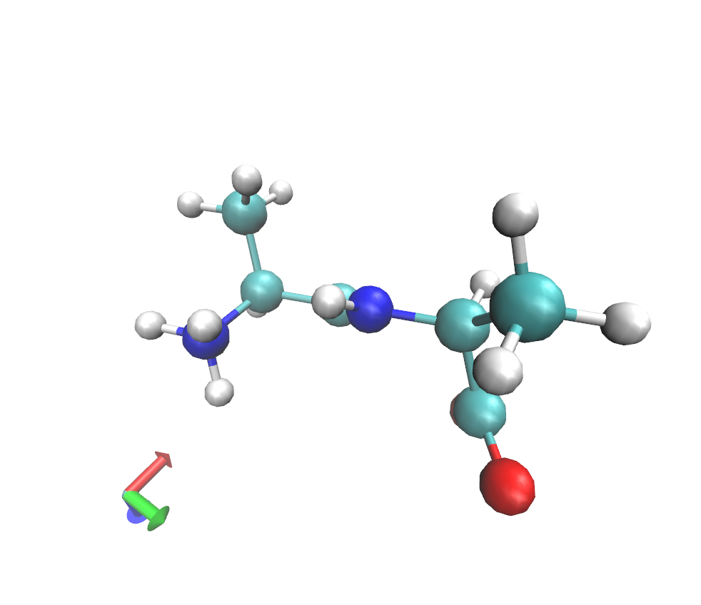
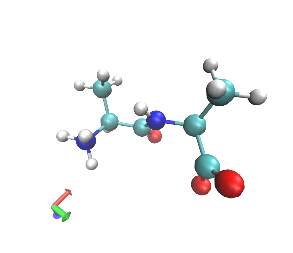
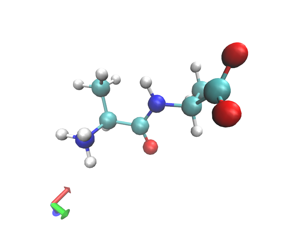
Figure 1: Snapshots from One Episode of Dialanine Folding

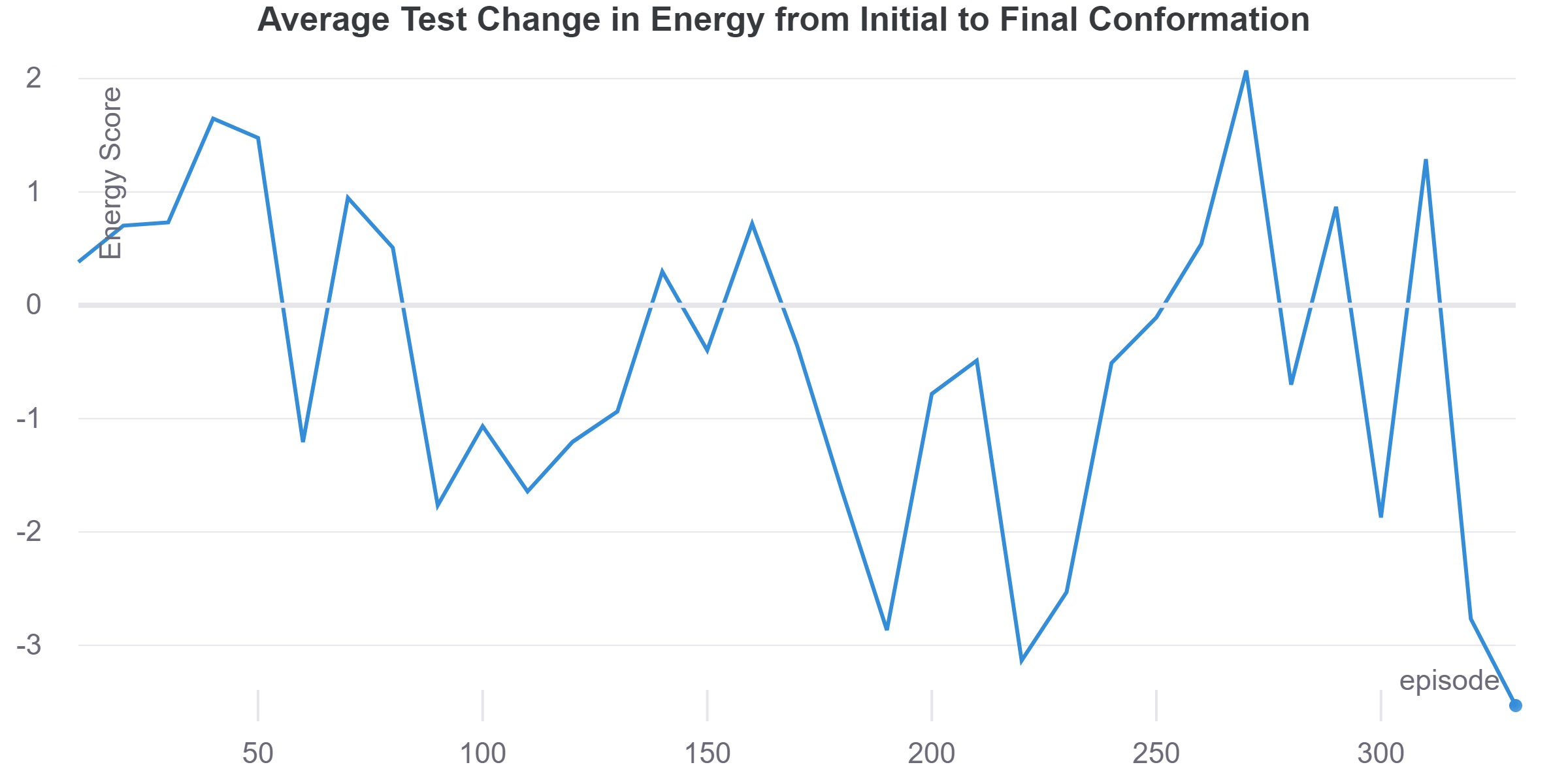
Figure 2: Average Change in Energy from Initial to Final Conformation at Test Time

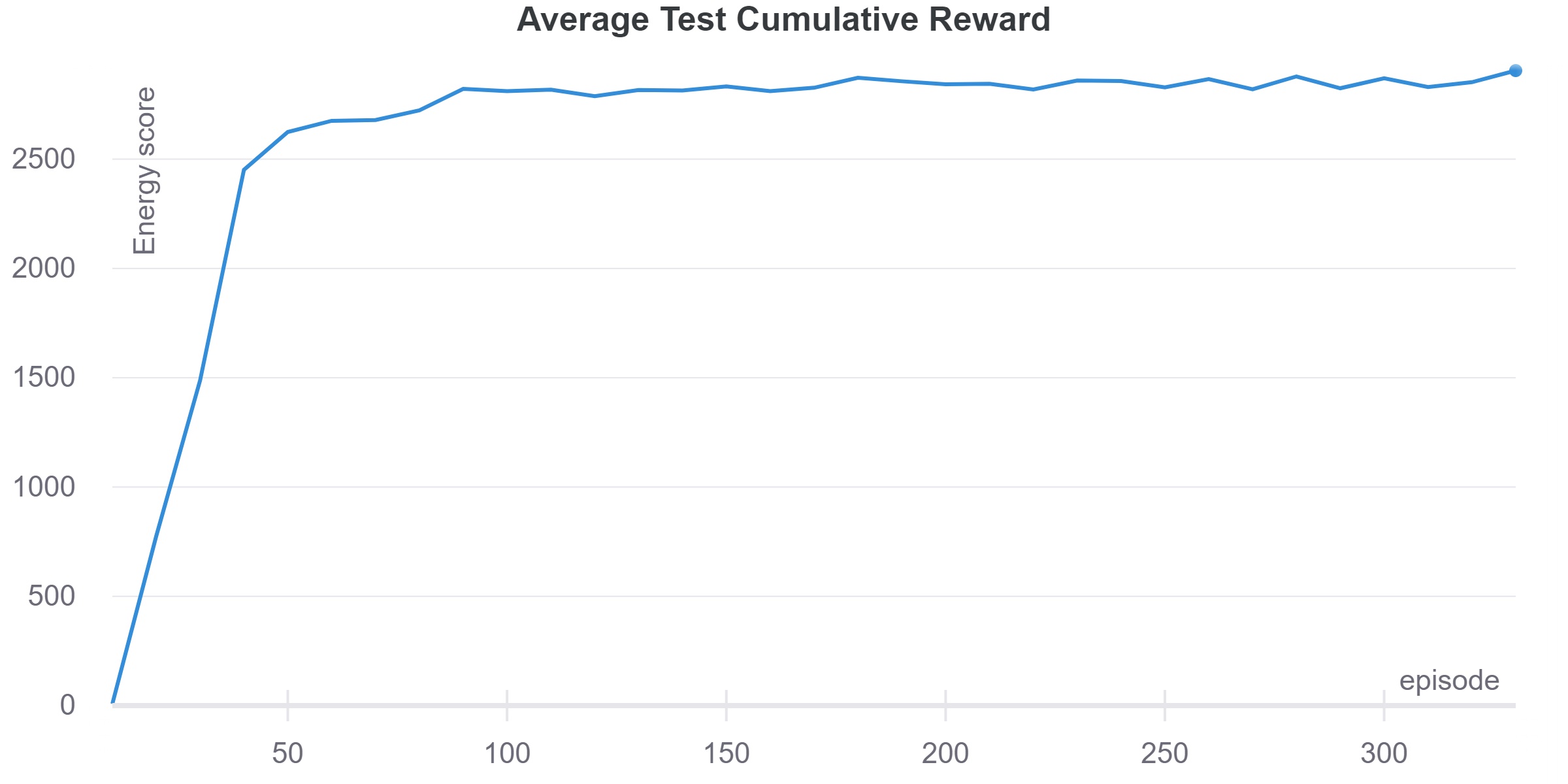
Figure 3: The Average Cumulative Reward at Evaluation Time

Figure 4: The Change in Energy at Training Time

4 Conclusions

In this paper, we learn the dihedral and/or rotamer angles of the optimal configuration of a protein structure by using a dynamic and continuous approach. The main continuous reinforcement learning formulation is derived from the stochastic Pontryagin’s maximum principle. Our algorithm is based on soft actor-critic and is guaranteed to converge to an optimal solution. Our optimal RL solution for a certain setting of our reward function and forward stochastic dynamics reduces to a general Langevin dynamics, which is considered as the suitable optimal dynamics for protein folding and structure prediction problems. We further show a variation of our formulation and its relation with the Nesterov’s accelerated gradient method. This suggests that one can use our general framework to derive further efficient reinforcement learning formulation for protein structure prediction and for learning dynamical systems in general.

5 Proofs of Lemma and Corollary

5.1 Proof of lemma 1

Proof.

By Pontryagin’s maximum principle, for the Hamiltonian $H(s,a,p,t)=p_{t}^{T}f(s_{t},a_{t})+l(s_{t},a_{t})$, we obtain the Hamiltonian system for the optimal trajectory $(s,a)=(s^{*},a^{*})$ (for simplicity we ignore the star notation):

$$ds =H_{p}(s(t),a(t),p(t),t)dt$$ (29)

$$dp =-H_{s}(s(t),a(t),p(t),t)dt$$ (30)

Moreover, $H_{a}(s(t),v,p(t),t)$ is minimized at $v=a(t)$ so that $H_{a}(s(t),a(t),p(t),t)=0$. Then for the dynamic function $f(s,a)=a$, and for the Lagrangian $l(x,u)=e^{\gamma t}(U(s)-a^{2}/2)$, we get:

$$p(t)+l_{a}(s_{t},a_{t})=0$$ (31)

Therefore, $p(t)=-l_{a}(s_{t},a_{t})=e^{\gamma t}a_{t}$. Plugging back into the dynamics of $p$, we get:

$$e^{\gamma t}(da+\gamma adt)=-l_{s}(s_{t},a_{t})dt=-e^{\gamma t}\nabla U(s_{t})dt$$ (32)

This yields the desired dynamics for 1 ∎

5.2 Proof of corollary 1

Proof.

By a similar proof to that of 1, we obtain the optimal trajectory $s_{t}$ with the following dynamics:

$$ds_{t} =a_{t}dt$$ (33)

$$da_{t} =-\gamma a_{t}dt-\nabla U(s_{t})dt-e^{-\gamma t}K_{t}dW_{t}$$ (34)

Because of the uniqueness of the solution to the adjoint stochastic differential equations 1, $e^{-\gamma t}K_{t}$ will be unique and must be the same as the constant in the Langevin dynamics because of the existence of the solution to the Langevin dynamics. Thus, this gives $e^{-\gamma t}K_{t}=K$ as desired. ∎

5.3 Further Enhancement

The Brownian motion term in equation 24 can be adjusted to better balance exploration and exploitation. To make this adjustment, we derived another formula based on our more general framework with stochastic Pontryagin maximum principle:

$$ds_{t} =a_{t}dt+\exp(-U(s_{t}))dW_{t}$$ (35)

$$da_{t} =-\gamma a_{t}dt-\nabla U(s_{t})dt$$ (36)

We still choose the same Lagrangian (or regret) function $l(s,a)=e^{\gamma t}(U(s)-a^{2}/2)$. For this formulation, the function $K$ in the Hamiltonian in equation 19 will become $0$. The function $u$ is now deterministic rather than a stochastic process as before. The proof is the same as that of the corollary 1. With this formulation, when the energy is large, the molecular agent dynamical process focuses more on exploitation and helps reduce the variance of the trajectory.

6 Trialanine Experiments

In addition to dialanine, we also tested our agent on the finding the minimal protein conformation for trialanine (i.e. three consecutively bonded alanines). Although the agent converged to a low energy conformation for trialanine, it did not converge to the global energy minimum. Moreover, thete

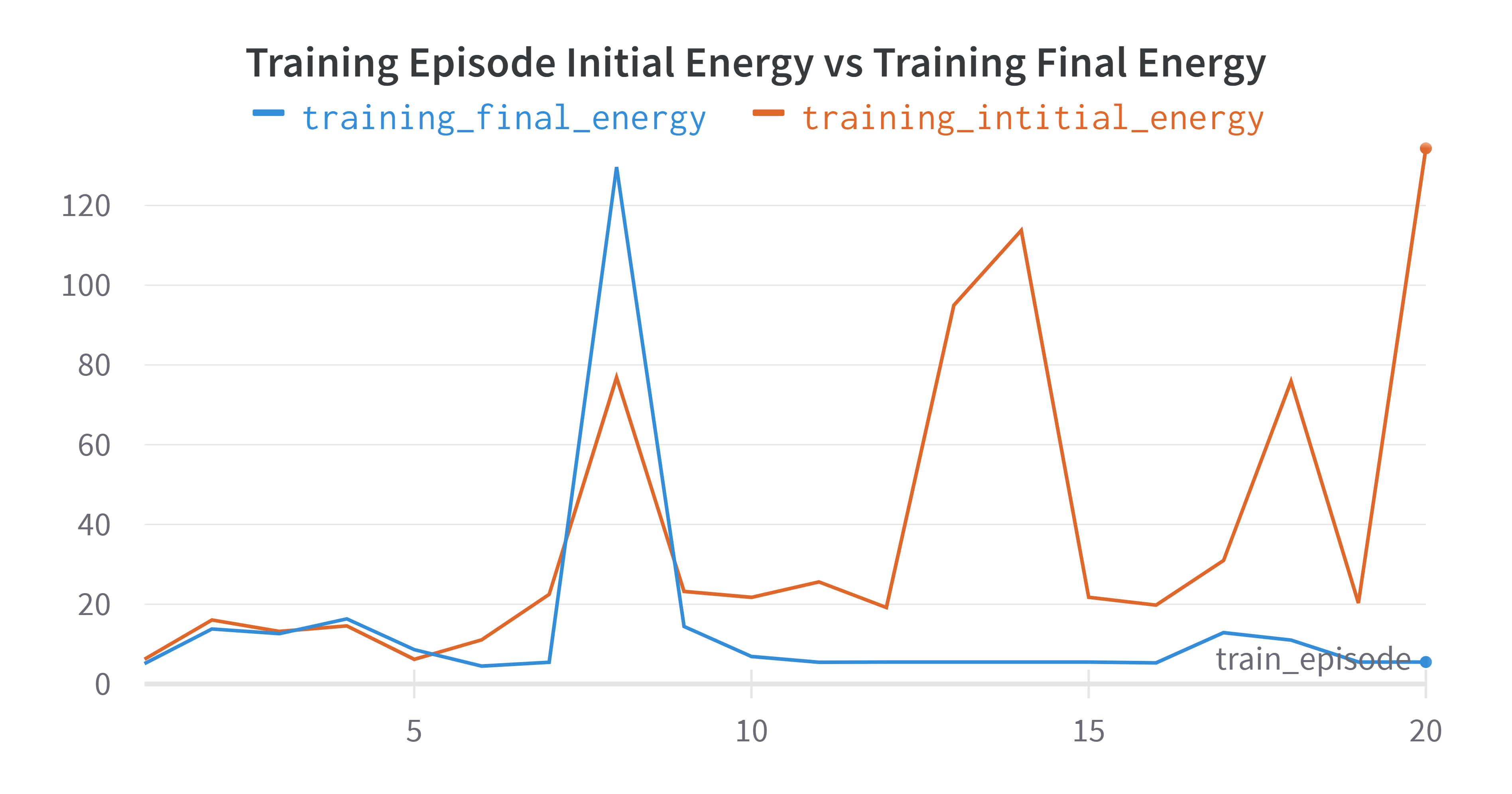
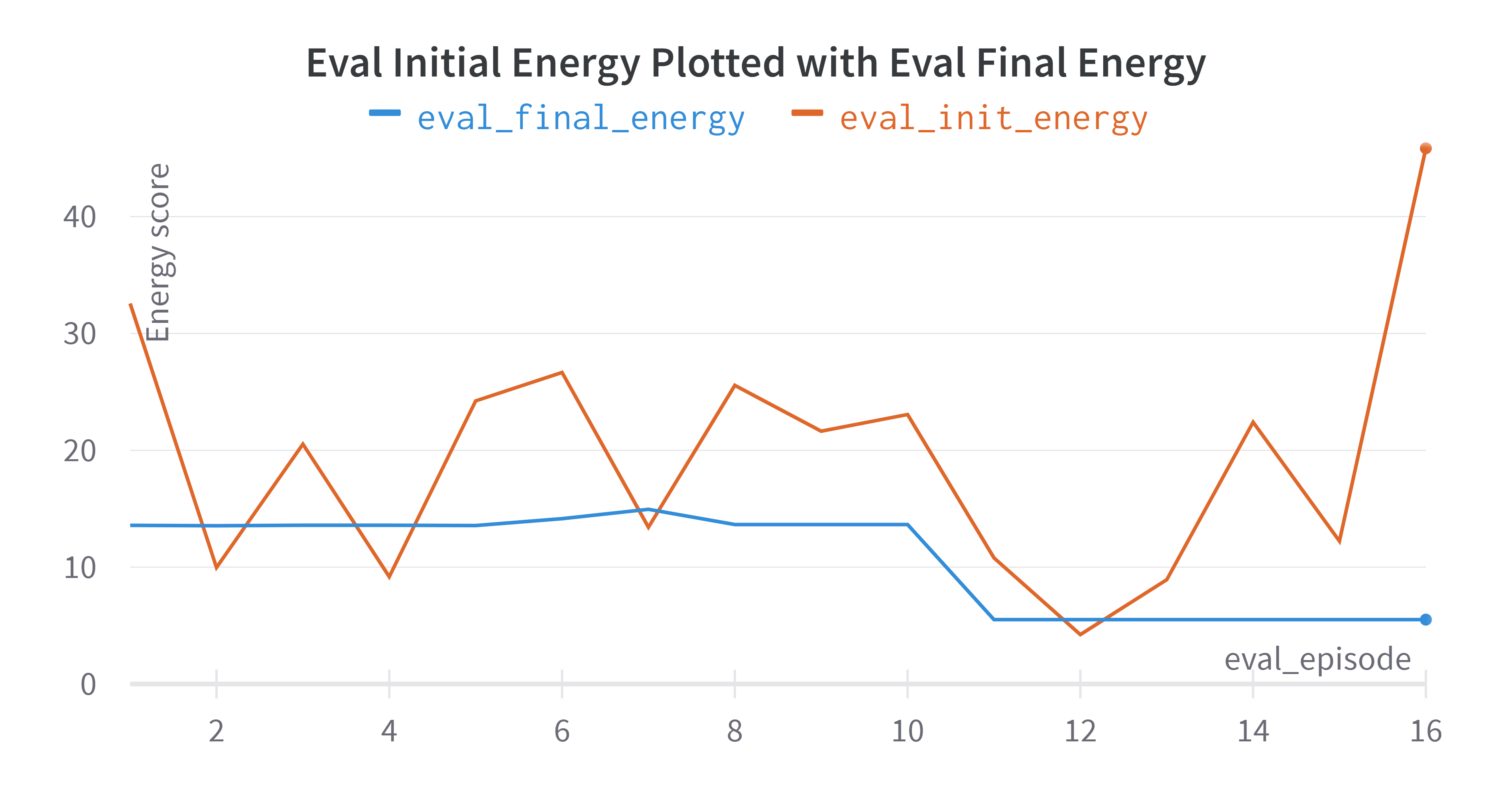
Figure 5: Initial vs final Energy plotted for each evaluation episode of trialanine

References

- [1] Tatsuya Akutsu. NP-hardness results for protein side-chain packing. In S. Miyano and T. Takagi, editors, Genome Informatics, volume 8, pages 180–186, 1997.
- [2] Niles A. Pierce and Erik Winfree. Protein design is NP-hard. Protein Eng., 15(10):779–782, 2002.
- [3] Bernard Chazelle, Carl Kingsford, and Mona Singh. A semidefinite programming approach to side chain positioning with new rounding strategies. INFORMS JOURNAL ON COMPUTING, 16(4):380–392, 2004.
- [4] Roland L. Dunbrack. Rotamer libraries in the 21st century. Current Opinion in Structural Biology, 12(4):431–440, 2002.
- [5] R. L. Dunbrack and F. E. Cohen. Bayesian statistical analysis of protein side-chain rotamer preferences. Protein Sci, 6(8):1661–1681, 1997.
- [6] Roland L. Dunbrack and Martin Karplus. Backbone-dependent rotamer library for proteins application to side-chain prediction. Journal of Molecular Biology, 230(2):543–574, 1993.
- [7] Roland L. Dunbrack and Martin Karplus. Conformational analysis of the backbone-dependent rotamer preferences of protein sidechains. Nat Struct Mol Biol, 1(5):334–340, 1994.
- [8] Simon C. Lovell, J. Michael Word, Jane S. Richardson, and David C. Richardson. The penultimate rotamer library. Proteins: Structure, Function, and Genetics, 40(3):389–408, 2000.
- [9] Marc De Maeyer, Johan Desmet, and Ignace Lasters. All in one: a highly detailed rotamer library improves both accuracy and speed in the modelling of sidechains by dead-end elimination. Folding and Design, 2(1):53–66, 1997.
- [10] Malcolm J. McGregor, Suhail A. Islam, and Michael J. E. Sternberg. Analysis of the relationship between side-chain conformation and secondary structure in globular proteins. Journal of Molecular Biology, 198(2):295–310, 1987.
- [11] Jay W. Ponder and Frederic M. Richards. Tertiary templates for proteins : Use of packing criteria in the enumeration of allowed sequences for different structural classes. Journal of Molecular Biology, 193(4):775–791, 1987.
- [12] P. Tuffery, C. Etchebest, S. Hazout, and R. Lavery. A new approach to the rapid determination of protein side chain conformations. J. Biomol.Struct. Dyn., 8:1267–1289, 1991.
- [13] Jinbo Xu. Rapid protein side-chain packing via tree decomposition. In Research in Computational Molecular Biology, pages 423–439. 2005.
- [14] Jinbo Xu and Bonnie Berger. Fast and accurate algorithms for protein side-chain packing. Journal of the ACM, 53(4):533–557, 2006. 1162350.
- [15] Shide Liang and Nick V. Grishin. Side-chain modeling with an optimized scoring function. Protein Sci, 11(2):322–331, 2002.
- [16] J. Mendes, A.M. Baptista, M.A. Carrondo, and C.M. Soares. Implicit solvation in the self-consistent mean field theory method: Side-chain modeling and prediction of folding free energies of protein mutants. J. Comp. Aided. Mol. Design, 5:721–740, 2001.
- [17] Zhexin Xiang and Barry Honig. Extending the accuracy limits of prediction for side-chain conformations. Journal of Molecular Biology, 311(2):421–430, 2001.
- [18] Johan Desmet, Marc De Maeyer, Bart Hazes, and Ignace Lasters. The dead-end elimination theorem and its use in protein side-chain positioning. Nature, 356(6369):539–542, 1992.
- [19] Johan Desmet, Marc De Maeyer, and Ignace Lasters. Theoretical and algorithmical optimization of the dead-end elimination theorem. In Pac. Symp. Biocomput., pages 122–133, 1997.
- [20] R. F. Goldstein. Efficient rotamer elimination applied to protein side-chains and related spin glasses. Biophys. J., 66(5):1335–1340, 1994.
- [21] D. Benjamin Gordon and Stephen L. Mayo. Branch-and-terminate: a combinatorial optimization algorithm for protein design. Structure, 7(9):1089–1098, 1999.
- [22] Donald A. Keller, Masayuki Shibata, Emil Marcus, Rick L. Ornstein, and Robert Rein. Finding the global minimum: a fuzzy end elimination implementation. Protein Eng., 8(9):893–904, 1995.
- [23] Ignace Lasters and Johan Desmet. The fuzzy-end elimination theorem: correctly implementing the side chain placement algorithm based on the dead-end elimination theorem. Protein Eng., 6(7):717–722, 1993.
- [24] Ignace Lasters, Marc De Maeyer, and Johan Desmet. Enhanced dead-end elimination in the search for the global minimum energy conformation of a collection of protein side chains. Protein Eng., 8(8):815–822, 1995.
- [25] Loren L. Looger and Homme W. Hellinga. Generalized dead-end elimination algorithms make large-scale protein side-chain structure prediction tractable: implications for protein design and structural genomics. Journal of Molecular Biology, 307(1):429–445, 2001.
- [26] N. A. Pierce, J. A. Spriet, J. Desmet, and S. L. Mayo. Conformational splitting: A more powerful criterion for dead-end elimination. Journal of Computational Chemistry, 21(11):999–1009, 2000.
- [27] Christopher A. Voigt, D. Benjamin Gordon, and Stephen L. Mayo. Trading accuracy for speed: a quantitative comparison of search algorithms in protein sequence design. Journal of Molecular Biology, 299(3):789–803, 2000.
- [28] Liisa Holm and Chris Sander. Database algorithm for generating protein backbone and side-chain co-ordinates from a C[alpha] trace : Application to model building and detection of co-ordinate errors. Journal of Molecular Biology, 218(1):183–194, 1991.
- [29] Andrej Sali and Tom L. Blundell. Comparative protein modelling by satisfaction of spatial restraints. Journal of Molecular Biology, 234(3):779–815, 1993.
- [30] Carleton L. Kingsford, Bernard Chazelle, and Mona Singh. Solving and analyzing side-chain positioning problems using linear and integer programming. Bioinformatics, 21(7):1028–1039, 2005.
- [31] Andrew R. Leach and Andrew P. Lemon. Exploring the conformational space of protein side chains using dead-end elimination and the a* algorithm. Proteins: Structure, Function, and Genetics, 33(2):227–239, 1998.
- [32] Christopher Lee and S. Subbiah. Prediction of protein side-chain conformation by packing optimization. Journal of Molecular Biology, 217(2):373–388, 1991.
- [33] Christopher Lee. Predicting protein mutant energetics by self-consistent ensemble optimization. Journal of Molecular Biology, 236(3):918–939, 1994.
- [34] K. C. D. Bahadur, E. Tomita, J. Suzuki, and T. Akutsu. Protein side-chain packing problem: a maximum edge-weight clique algorithmic approach. Journal of Bioinformatics and Computational Biology, 3:103–126, 2005.
- [35] E. Althaus, O. Kohlbacher, H. Lenhof, and P Müller. A combinatorial approach to protein docking with flexible side-chains. In Fourth Annual International Conference on Computational Molecular Biology, pages 15–24. ACM Press, 2000.
- [36] Olivia Eriksson, Yishao Zhou, and Arne Elofsson. Side chain-positioning as an integer programming problem. In Algorithms in Bioinformatics, pages 128–141. 2001.
- [37] Ke Liu, Xiangyan Sun, Jun Ma, Zhenyu Zhou, Qilin Dong, Shengwen Peng, Junqiu Wu, Suocheng Tan, Günter Blobel, and Jie Fan. Prediction of amino acid side chain conformation using a deep neural network, 2017.
- [38] Ken Nagata, Arlo Randall, and Pierre Baldi. Sidepro: A novel machine learning approach for the fast and accurate prediction of side-chain conformations. Proteins: Structure, Function, and Bioinformatics, 80(1):142–153, 2012.
- [39] Mohammed AlQuraishi. End-to-end differentiable learning of protein structure. Cell Systems, 8(4):292 – 301.e3, 2019.
- [40] Mohammed AlQuraishi. Proteinnet: a standardized data set for machine learning of protein structure. BMC Bioinformatics, 20(1):311, 2019.
- [41] Andrew W. Senior, Richard Evans, John Jumper, James Kirkpatrick, Laurent Sifre, Tim Green, Chongli Qin, Augustin Žídek, Alexander W. R. Nelson, Alex Bridgland, Hugo Penedones, Stig Petersen, Karen Simonyan, Steve Crossan, Pushmeet Kohli, David T. Jones, David Silver, Koray Kavukcuoglu, and Demis Hassabis. Improved protein structure prediction using potentials from deep learning. Nature, 577(7792):706–710, 2020.
- [42] John Jumper, Richard Evans, Alexander Pritzel, Tim Green, Michael Figurnov, Olaf Ronneberger, Kathryn Tunyasuvunakool, Russ Bates, Augustin Žídek, Anna Potapenko, Alex Bridgland, Clemens Meyer, Simon A. A. Kohl, Andrew J. Ballard, Andrew Cowie, Bernardino Romera-Paredes, Stanislav Nikolov, Rishub Jain, Jonas Adler, Trevor Back, Stig Petersen, David Reiman, Ellen Clancy, Michal Zielinski, Martin Steinegger, Michalina Pacholska, Tamas Berghammer, Sebastian Bodenstein, David Silver, Oriol Vinyals, Andrew W. Senior, Koray Kavukcuoglu, Pushmeet Kohli, and Demis Hassabis. Highly accurate protein structure prediction with alphafold. Nature, 596(7873):583–589, Aug 2021.
- [43] John Ingraham, Adam Riesselman, Chris Sander, and Debora Marks. Learning protein sturcture with a differentiable simulator. In ICLR, 2019.
- [44] Reza Jafari and Mohammad Masoud Javidi. Solving the protein folding problem in hydrophobic-polar model using deep reinforcement learning. SN Appl. Sci., 2(2), 2020.
- [45] Kit Fun Lau and Ken A Dill. A lattice statistical mechanics model of the conformational and sequence spaces of proteins. Macromolecules, 22(10):3986–3997, 1989.
- [46] Hongjie Wu, Ru Yang, Qiming Fu, Jianping Chen, Weizhong Lu, and Haiou Li. Research on predicting 2D-HP protein folding using reinforcement learning with full state space. BMC Bioinformatics, 20(Suppl 25):685, 2019.
- [47] Shige Peng. A general stochastic maximum principle for optimal control problems. SIAM j. control optim., 28(4):966–979, 1990.
- [48] Jordi Grau-Moya, Felix Leibfried, and Peter Vrancx. Soft q-learning with mutual-information regularization. In International Conference on Learning Representations, 2019.
- [49] Weijie Su, Stephen Boyd, and Emmanuel J Candes. A differential equation for modeling nesterov’s accelerated gradient method: Theory and insights. 2015.
- [50] Rebecca F. Alford, Andrew Leaver-Fay, Jeliazko R. Jeliazkov, Matthew J. O’Meara, Frank P. DiMaio, Hahnbeom Park, Maxim V. Shapovalov, P. Douglas Renfrew, Vikram K. Mulligan, Kalli Kappel, Jason W. Labonte, Michael S. Pacella, Richard Bonneau, Philip Bradley, Roland L Dunbrack Jr., Rhiju Das, David Baker, Brian Kuhlman, Tanja Kortemme, and Jeffrey J. Gray. The rosetta all-atom energy function for macromolecular modeling and design. Journal of chemical theory and computation, 13(6):3031–3048, Jun 2017. 28430426[pmid].
- [51] Tuomas Haarnoja, Aurick Zhou, Pieter Abbeel, and Sergey Levine. Soft actor-critic: Off-policy maximum entropy deep reinforcement learning with a stochastic actor. In ICML, 2018.
- [52] Nicola De Cao and Thomas Kipf. Molgan: An implicit generative model for small molecular graphs, 2018.
- [53] Daniel Ting, Guoli Wang, Maxim Shapovalov, Rajib Mitra, Michael I. Jordan, and Roland L. Dunbrack, Jr. Neighbor-dependent ramachandran probability distributions of amino acids developed from a hierarchical dirichlet process model. PLOS Computational Biology, 6:1–21, 04 2010.