The prevalence and influence of circumstellar material around hydrogen-rich supernova progenitors

Abstract

Narrow transient emission lines (flash-ionization features) in early supernova (SN) spectra trace the presence of circumstellar material (CSM) around the massive progenitor stars of core-collapse SNe. The lines disappear within days after the SN explosion, suggesting that this material is spatially confined, and originates from enhanced mass loss shortly (months to a few years) prior to explosion. We performed a systematic survey of H-rich (Type II) SNe discovered within less than two days from explosion during the first phase of the Zwicky Transient Facility (ZTF) survey (2018-2020), finding thirty events for which a first spectrum was obtained within $<2$ days from explosion. The measured fraction of events showing flash ionisation features ($>36\%$ at $95\%$ confidence level) confirms that elevated mass loss in massive stars prior to SN explosion is common. We find that SNe II showing flash ionisation features are not significantly brighter, nor bluer, nor more slowly rising than those without. This implies that CSM interaction does not contribute significantly to their early continuum emission, and that the CSM is likely optically thin. We measured the persistence duration of flash ionisation emission and find that most SNe show flash features for $\approx 5$ days. Rarer events, with persistence timescales $>10$ days, are brighter and rise longer, suggesting these may be intermediate between regular SNe II and strongly-interacting SNe IIn.

1 Introduction

Early observations of Type II supernovae (SNe II) reveal that a large fraction shows transient narrow emission lines of highly-ionised species (Khazov et al. 2016; Bruch et al. 2021). Such lines may result either from the recombination of slowly expanding circumstellar medium (CSM) excited and ionised by the SN shock breakout and the shock-cooling emission (Yaron et al., 2017; Gal-Yam et al., 2014; Niemela et al., 1985); or from the recombination of unshocked CSM excited by radiation originating from shocks driven by underlying ejecta-CSM interaction. The former excitation mechanism is called flash ionisation (Gal-Yam et al., 2014), while the latter would better be described by shock ionisation (Terreran et al., 2022). After a few days, in both cases, these lines disappear, which suggests that the CSM is confined to a small volume around the progenitor, and is swept up by the ejecta.

Follow-up observations (e.g. rapid-response spectroscopy and multiband photometry, Gal-Yam et al. 2011) are useful to probe the properties of the progenitor and its surroundings. For example, Rabinak & Waxman (2011) (RW11, hereafter) motivate acquiring daily multiband photometry at early times to constrain the radius of the progenitor as well as the explosion energy per unit mass. The RW11 model is no longer valid once the recombination phase has started, which is marked by the emergence of broad hydrogen P-Cygni-like lines. Rapid-response spectroscopy with a day cadence is hence needed to identify the beginning of the recombination phase. As we show below, detecting narrow emission lines at early time is indicative of interaction with CSM, which could also invalidate the use of such models. Studies of large samples of such events are important to establish the characteristic SN progenitor channels and the conditions which bring them to explosion.

Signatures of a dense and extended CSM are observed in Type IIn SNe. These are hydrogen rich SNe that show strong and narrow Balmer emission lines for an extended period of time and do not develop broad hydrogen features, characteristic of the high expansion velocity of the SN ejecta around peak light (Schlegel 1990; Filippenko 1997; Kiewe et al. 2012; Smith 2014). The narrow features come from slowly expanding CSM, energized from within by the shock interaction between the expanding ejecta and dense CSM, (Chugai & Danziger 1994). Such interaction can last from weeks to years after the explosion. Photometrically, SNe IIn are typically brighter (M${}_{peak,\text{r}}\approx-19$ mag) and can rise to peak on longer timescales ($t_{rise,\text{r}}>20$d) than SNe II (M${}_{peak,\text{r}}\approx-17.5$ mag and $t_{rise,\text{r}}<20$d, respectively), see Nyholm et al. (2020) for SNe IIn and Rubin et al. (2016) for SNe II. This extra luminosity is thought to come from the interaction with the CSM. Indeed, the kinetic energy from the ejecta is converted to X-Rays via collisionless shocks in the CSM, and then converted to visible light if enough optical depth is present.

The origin of this CSM is usually attributed to an elevated mass loss prior to the explosion. Indeed, massive stars are known to experience mass loss throughout their lives ($\dot{M}<10^{-4}M_{\odot}$.year^-1 for red supergiants (RSG), see chapter 8 in Prialnik (2009) and Figure 3 in Smith (2016)). However, there is also evidence for episodic elevated mass-loss just prior to the explosion (Ofek et al., 2013, 2014; Strotjohann et al., 2021; Jacobson-Galán et al., 2022). Such precursor emission with enhanced mass-loss could originate from strong convection close to the core, in the late stages of nuclear burning, which generates waves that heat the stellar envelope intensively (Quataert & Shiode, 2012; Shiode & Quataert, 2014). Other ideas involve for example sudden energy release in deep layers of the stars from late-stage nuclear burning instabilities (Meakin & Arnett, 2007). For SNe IIn, the CSM distribution requires extensive mass loss over a long period of time (years prior explosion, see Strotjohann et al. (2021); Ofek et al. (2013, 2014)). In the case of flash features, the CSM presumably lies in a more confined space and could result from mass-loss episodes, occurring shortly prior to the explosion (Gal-Yam et al., 2014; Yaron et al., 2017; Jacobson-Galán et al., 2022).

Since CSM shock interaction seems to power the light curve of SNe IIn, it is possible that CSM interaction contributes also to the early light curve of SNe II with a confined CSM shell, (Morozova et al., 2017). Thus we expect that SNe II with CSM reach higher luminosities than those without CSM, as hypothesised in Hosseinzadeh et al. (2018).

We present here a systematic search for flash-ionisation features in hydrogen-rich SNe shortly after explosion ($<2.5$  days). In Section 2, we describe our construction of a large sample of infant SNe and our observations. In section 3, we present our analysis, and thus discuss our results in section 4. We conclude in section 5.

In this paper, we assume cosmology parameters from Planck Collaboration et al. 2014, which yields a Hubble constant at $H_{0}=67.3\pm 1.2\,$ km.Mpc^-1.s^-1. Magnitudes are given in the AB system. The photometry and spectra presented in this paper will be made public through WiseRep (Yaron & Gal-Yam 2012).

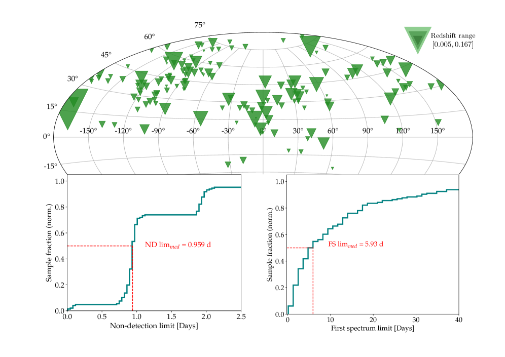
Figure 1: Sample statistics: celestial distribution of the 148 candidates of the real-infant sample. Large triangles designate low redshift events, smaller ones higher redshift. Our sample ranges from $z=0.005$ to $z=0.167$ Bottom left: Non-detection limit distribution. Half of the sample was discovered within $0.9\,\text{days}$ of the last non-detection. Bottom right: Time of the first spectrum. 22% of the sample has a first spectrum within less than 2.5d the last non-detection.

2 Observations

2.1 Sample construction

We constructed our sample through both real-time data scanning and complementary archival search. We consider SNe detected and classified by ZTF-I, i.e. between March 2018 and December 2020, and restrict our search to spectroscopically-classified SN II, IIn and IIb. A candidate is considered spectroscopically classified if at least one spectrum exists on the ZTF Growth Marshal (Kasliwal et al., 2019). To constrain non-detection limits, we consider exclusively the light curves provided by P48. We compute the non-detection limits from the light curves of 1252 spectroscopically-classified hydrogen rich SNe and find that 425 have a non-detection within $<2.5$ days from the first detection. We carried out forced photometry for the candidate sample composed of these 425 H-rich candidates. At this stage, the light curves were not corrected for extinction or redshift.
A candidate is qualified as a ”Real Infant” SN if for a given filter (r and/or g) there is a non-detection within $<2.5$ days, and if the magnitude rise above the limiting magnitude of this non-detection is $>0.5$ magnitudes, as described in Bruch et al. (2021).
Forced photometry is more sensitive than the ZTF alert detection pipeline (see Yao et al. 2019) and some initially reported non-detections turn into faint detections (e.g.: SN 2019eoh) and reveal an intra-night rise $>0.5$ mag. Such fast rising behaviour is characteristic of an infant SN and we therefore also add events with an intra-night rise of at least 0.5 magnitudes in the same band to our sample.

Some SNe were mistakenly classified as Type IIn SNe, based on early spectra where narrow hydrogen lines could be flash ionisation lines. Some candidates, such as SN 2019qch, were classified as a SN IIn based on long lasting flash ionisation features. This SN developed a classic broad P-Cygni profile, characteristic of spectroscopically normal SNe II later. Whenever an event was classified as a SNe IIn, but showed this latter behaviour, we changed the classification to SN II.

The final sample (see Tables 6,9,10 in the Annex) is composed of 148 SNe discovered between March 2018 and December 2020. The median non-detection limit from the first detection is 0.9 days. The median acquisition of a first spectrum from the last non detection is $\approx 6$ days, see Figure 1.

2.2 Photometry

Alert system photometry from P48

We had access to the partnership and public photometric data stream from ZTF (Bellm et al., 2019; Graham et al., 2019; Dekany et al., 2020). We used this pipeline and its real-time alert distribution via the GROWTH marshal to look for infant candidates on a daily basis. We complementary used the AMPEL system for filtering the incoming alerts, (Nordin et al., 2019; Soumagnac & Ofek, 2018).

Real time forced photometry bot

During the scanning campaign, we also used the fpbot (Reusch, 2022). The fpbot returns in real time the forced photometry of a ZTF object and sends it to the platform Slack. Such a service was useful upon the discovery of a candidate to ensure that the first detection was real prior to triggering spectroscopic follow up.

Forced photometry

We carried out forced photometry for the entirety of our sample and applied the quality cuts described in Bruch et al. (2021). We visually inspect the resulting magnitude light curves from forced photometry as well as the alert system photometry to determine the first detection and last non-detection. We retrieved pre-discovery detections from the forced photometry magnitude light curves for 53 candidates . The median value is 0.99 days prior to the detection from the alert system. From this point on, we use the first detection and last non-detection from the forced-photometry light curves. Some candidates from 2020 have measurements from Caltech-partnership data stream. Since we did not have access to them at the time of the analysis, they are not included in this study. This does not impact significantly our analysis. It was established in Bellm et al. (2019) that the ZTF single image limit is on average 21 magnitude. We hence remove any detections from the forced photometry which are below 21st magnitude. The forced-photometry light curves can be found in Table 1.

Table 1: Forced-photometry light curves of the 148 events in our Real Infant sample. The full version can be found online.

Time from	Time	Flux	Flux	Apparent	$\delta$m	Absolute	$\delta$M	Filter	ZTF
EED			error	magnitude		magnitude			name
	[JD]	$10^{-8}$[Mgy]	$10^{-8}$[Mgy]	(m)		(M)
…	…	…	…	…	…	…	…	…	…
17.420	2458898.817	4.97484548	0.16902504	18.26	0.04	-17.74	0.04	r	ZTF18aaaibml
18.404	2458899.801	5.09761181	0.14810007	18.23	0.03	-17.76	0.03	r	ZTF18aaaibml
20.478	2458901.875	4.67906920	0.13268852	18.32	0.03	-17.67	0.03	r	ZTF18aaaibml
22.413	2458903.810	4.40633990	0.12260471	18.39	0.03	-17.60	0.03	g	ZTF18aaaibml
23.330	2458904.727	5.04859332	0.15628758	18.24	0.03	-17.75	0.03	r	ZTF18aaaibml
23.377	2458904.774	3.85174173	0.10942362	18.54	0.03	-17.46	0.03	g	ZTF18aaaibml
…	…	…	…	…	…	…	…	…	…

2.3 Spectroscopy

Our goal was to obtain rapid spectroscopy of infant SN candidates following the methods of Gal-Yam et al. (2011). This was made possible using rapid ToO follow-up programs as well as on-request access to scheduled nights on various telescopes. During the active search for new transients, we applied the following criteria for rapid spectroscopic triggers: The robotic SEDm (see below) was triggered for all candidates brighter than a magnitude threshold of $19$ mag. The co-location of the P60 and ZTF/P48 on the same mountain, as well as the P60 robotic response capability, enable rapid, often same-night, response to ZTF events. However, the low resolution ($R\sim 100$) of the instrument limits our capability to characterise narrow emission lines. This, along with the overall sensitivity of the system, motivated us to obtain higher-resolution follow-up spectroscopy with larger telescopes, particularly for all infant SNe fainter than $r\sim 19$ mag at discovery. Higher-resolution spectra (using WHT, Gemini, or other available instruments) were triggered for events assured to be of extragalactic nature , showing recent non-detection limits (within $2.5$ d prior to first detection) as well as a significant brightening compared to a recent non-detection.

We present here the spectroscopic facilities we used during our search for infant SNe II.

P60/SEDm

The Spectral Energy Distribution Machine (SEDm; Ben-Ami et al. (2012); Blagorodnova et al. (2018); Neill (2019)) is a high-throughput, low-resolution spectrograph mounted on the 60” robotic telescope (P60; Cenko et al. (2006)) at Palomar observatory. $65\%$ of the time on the SEDm was dedicated to ZTF partnership follow up. SEDm data are reduced using an automated pipeline (Rigault et al., 2019; Kim et al., 2022).

LT/SPRAT

We used the Spectrograph for the Rapid Acquisition of Transients (SPRAT; Piascik et al. (2014)). It is a highthroughput, low-resolution spectrograph mounted on the Liverpool Telescope (LT; 58), a 2 meter robotic telescope at the Observatorio del Roque de Los Muchachos in Spain. All the spectra were reduced using the standard pipeline provided by the observatory.

P200/DBSP

We used the Double Beam SPectrograph (DBSP; Oke & Gunn (1982)) mounted on the 5m Hale telescope at Palomar Observatory (P200) to obtain follow-up spectroscopy in either ToO mode or during classically-scheduled nights. The default configuration used the 600/4000 grism on the blue side, the 316/7150 grating on the red side, along with the D55 dichroic, achieving a spectral resolution $R\sim 1000$. Spectra obtained with DBSP were reduced using the pyraf-dbsp pipeline (Bellm & Sesar, 2016).

WHT/ISIS&ACAM

We obtained access to the 4.2m William Herschel Telescope (WHT) at the Observatorio del Roque de los Muchachos in La Palma, Spain, via the Optical Infrared Coordination Network for Astronomy (OPTICON) program. We used both single-slit spectrographs ISIS and ACAM (Benn et al., 2008) in ToO service observing mode. The delivered resolutions were $R\sim 1000$ and $R\sim 400$, respectively. Spectral data were reduced using standard routines within IRAF .

Keck/LRIS

We used the Low-Resolution Imaging Spectrometer (LRIS; Oke et al. (1995)) mounted on the Keck-I 10m telescope at the W. M. Keck Observatory in Hawaii in either ToO mode or during scheduled nights. The data were reduced using the LRIS automated reduction pipeline Lpipe (Perley, 2019).

GMOS/Gemini

We used the Gemini Multi-Object Spectrograph (GMOS; Hook et al. 2004) mounted on the Gemini North 8m telescope at the Gemini Observatory on Mauna Kea, Hawaii. All observations were conducted at a small airmass ($\lesssim 1.2$). For each SN, we obtained 2$\times$900 s exposures using the B600 grating with central wavelengths of $520$ nm and $525$ nm. The $5$ nm shift in the effective central wavelength was applied to cover the chip gap, yielding a total integration time of $3600$ s. A 1.0$\arcsec$-wide slit was placed on each target at the parallactic angle. The GMOS data were reduced following standard procedures using the Gemini IRAF package.

ARC/DIS

We used the Dual Imaging Spectrograph (DIS) on the Astrophysical Research Consortium (ARC) 3.5 m telescope at Apache Point Observatory (APO) during scheduled nights. The data were reduced using standard procedures and calibrated to a standard star obtained on the same night using the PyDIS package (Davenport, 2018).

NOT/ALFOSC

Some data presented here were obtained with the Andalucia Faint Object Spectrograph and Camera (ALFOSC) mounted on the 2.56 meter Nordic Optical Telescope (NOT)

VLT/FORS2

Some data presented here were obtained with the FOcal Reducer/low dispersion Spectrograph 2 on the Very Large Telescope in Long Slit spectroscopic mode. The data were obtained as part of the adH0cc project, based on the ESO-VLT Large Programme 1104.A-0380.

VLT/X-Shooter

Some data presented here were obtained with X-Shooter (Vernet et al. (2011)) as part of the ToO programme for Infant Supernovae. Optical spectra were obtained with the VIS spectrograph with an exposure time of $1450$s.
The data were reduced following Selsing et al. (2019). In brief, we first removed cosmic-rays with the tool astroscrappy, which is based on the cosmic-ray removal algorithm by van Dokkum (2001). Afterwards, the data were processed with the X-shooter pipeline v3.3.5 and the ESO workflow engine ESOReflex (Goldoni et al., 2006; Modigliani et al., 2010). The UVB and VIS-arm data were reduced in stare mode to boost the S/N by a factor of $\sqrt{2}$ compared to the standard nodding mode reduction. The individual rectified, wavelength- and flux-calibrated two-dimensional spectra files were co-added using tools developed by J. Selsing.

The classification spectra of each SN can be found on the Transient Name Server.

3 Analysis

Since our goal is to compare the photometric and spectroscopic behaviour of SNe II showing flash features and SNe II that do not, we need to estimate the explosion time, peak magnitude and rise time for each SN. We also discuss the identification of flash ionisation features in early spectra of SNe II.

3.1 Explosion time estimation

We use the fitter iminuit (Dembinski et al. 2020) to fit the empirical function $f(t)=a\times(t-t_{exp})^{n}$, where $f(t)$ is the SN flux and $t_{exp}$ the time of zero flux. For each SN, we fit data from $-10$ until $2.5$, $3.5$, $4.5$ and $5.5$ days from first detection in $r$ and $g$ band. We inspect each fit visually. Whenever more than two fits (per band) were of poor quality, we adopted the time of zero flux as the mid point between the last non-detection limit and the first detection . We consider fits poor if they do not converge or if there are fewer than three observations after the first detection. We measure here the observer’s time of zero flux and present it as the estimated explosion date (EED).

3.2 Peak magnitude estimation

Using the methods described in Bruch et al. (2021), we estimate the peak magnitude: we correct the light curve for Milky Way extinction and redshift and fit a third degree polynomial to the light curve around the visual maximum. We repeat the fitting procedure 100 times and randomly vary the start and end dates of the fit. We estimate the value of the peak as the median of the maximum values. The rise time is the time from the estimated explosion date (EED) to the measured maximum. The error on the absolute peak magnitude is:

$$\delta M_{peak}=\sqrt{\delta m_{peak}^{2}+\delta\mu^{2}}$$ (1)

with $\delta m_{peak}$, the standard deviation on the peak magnitude measurements and $\delta\mu$ is the error on the distance modulus, calculated from the error on the redshift as: $\delta\mu=\frac{5\delta z}{ln(10)\times z}$.

3.3 Light curve interpolation

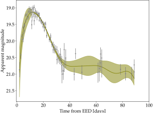
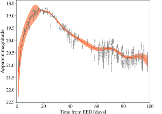
Figure 2: Full lightcurve interpolation of e.g. ZTF18abcezmh in the $g$ band (up) and $r$ band (down). The colored band represents the error on the interpolation from either the early time fit or the Gaussian process interpolation.

We also want to compare the colour at peak of each SN. We hence need to interpolate the light curve in each band. We divide the light curve into two parts: the rise and the decline. The rise is fit by either a simple exponential law or a broken power law until the estimated peak flux. The decline is fit using gaussian processes. We use the forced-photometry light curves corrected for galactic extinction and redshift.

The rising lightcurve usually shows a fast rise followed by a slower rise. We use either a simple exponential law or a broken power law inspired by Equation (2) in Jóhannesson et al. (2006). Indeed, a simple exponential law is not enough in some cases to fit the full rise from EED to peak. The best fit is determined by a $\chi^{2}$ test. We fit the rise in flux space. Both functions are bounded to the estimated peak flux at the estimated peak time. The simple power law can be written as:

$$F=-A\left(-\left(t-t_{peak}\right)\right)^{n}+F_{peak}$$ (2)

The broken power law is given by:

$$F=-A\left(\left(\frac{-(t-t_{peak})}{t_{break}}\right)^{-\alpha_{1}}+\left(\frac{-(t-t_{peak})}{t_{break}}\right)^{-\alpha_{2}}\right)+F_{peak}$$ (3)

Where $F_{peak}$, $t_{peak}$ are respectively the peak flux and rise time, and $t_{break}$ is the time where the transition between the two power laws happens. We use the Minuit optimiser, based on a least-square test, to choose which law fits best in each case. We then convert the obtained interpolation from flux space to magnitude space.

We use Gaussian processes to interpolate the decline part of the lightcurve. In order to estimate the overall decrease of magnitude per day after peak, we fit a linear function to the light curve after the estimated peak :

$$mag=a\times(t-t_{peak})+m_{peak}$$ (4)

We exclude data points below 21 st magnitude and visually select the end of the region we choose to fit (usually $\approx 40$ days), usually corresponding to the last measurements before the SN is not observable anymore. We use this estimated linear decline curve as the mean function for Gaussian processes interpolation.

Gaussian processes are not suitable to interpolate early SN light curves because they require a kernel that quantifies on what time scales the entire light curve varies. Indeed, Gaussian processes utilise a set of priors on the characteristic behaviour of the data. These priors are encapsulated in the Kernel from which each random function is drawn. One of the most basic assumptions for the Kernel is the characteristic size and amplitude of variation, i.e. two datapoints separated by length x have a correlated behaviour and can vary over A range of amplitude. For us, the characteristic length for two points to behave alike is time, and the amplitude is some range of magnitude. From explosion to peak, very young Cor-Collapse SNe (CC SNe) first rise within hours, but, as the ejecta have expanded to a larger radius, they then vary over much longer time scales. There is therefore no single characteristic time scale for this phase, and hence for the full lightcurve. However, in the linear decline phase from peak, we can assume that the characteristic timescale throughout the decline phase is almost constant. We choose this time to be $\tau\approx 100$ days. The full light curve interpolation is stitched together at the estimated peak mag and time. See Figure 2 for an example.

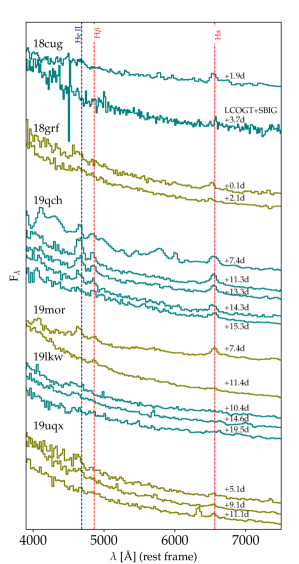
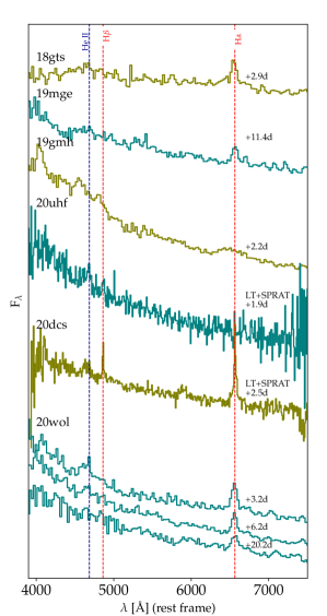
Figure 3: Collection of flash ionisation features spectra for the low-resolution group. Unless written otherwise, spectra were observed with SEDm+P60. The times indicated on the red side of the spectra correspond to the time of acquisition of the spectra from the estimated explosion date.

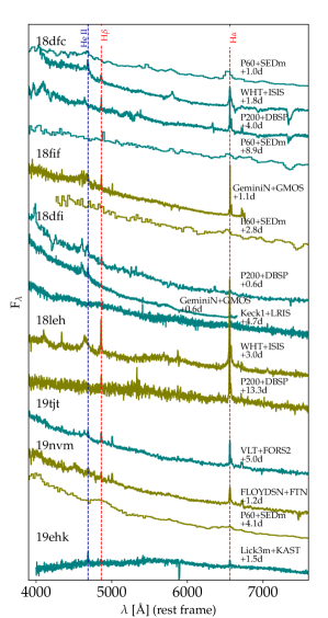
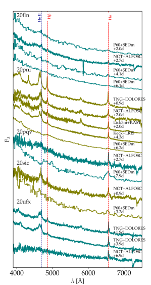
Figure 4: Collection of flash ionisation features spectra for the high-resolution group. The times indicated on the red side of the spectra correspond to the time of acquisition of the spectra from the estimated explosion date.

3.4 Subclassification of SNe II

Following Gal-Yam (2017), we sub-classify our sample in three categories: spectroscopically-normal SNe II, interacting SNe IIn and helium-rich SNe IIb. Spectroscopically-normal SNe II develop a high velocity ($\approx 10000$  km.s^-1) Balmer P-Cygni profile in the photospheric phase. We do not consider here the photometric subclassifications of SNe IIP or IIL. SNe IIn show narrow Balmer emission lines which last for several weeks. SNe IIb develop early on strong absorption lines of He I.

3.5 Flash features in SNe II

IAU	Type	Flasher	Instrument+Telescope	Time to	Spectrograph
name			(of first spectrum)	first spectrum	Resolution
(SN)				from EED
				[days]
2018grf	SN II	yes	SEDm+P60	0.14	low
2019nvm	SN II	yes	SEDm+P60	0.17	low
2018dfi	SN IIb	yes	DBSP+P200	0.60	high
2020pni	SN II	yes	DOLORES+TNG	0.86	high
2020sic	SN II	yes	ALFOSC+NOT	0.89	high
2018dfc	SN II	yes	SEDm+P60	1.02	low
2018fif	SN II	yes	DBSP+P200	1.13	high
2019ehk	SN IIb	yes	KAST+Lick	1.47	high
2018cyg	SN II	yes	ACAM+WHT	1.68	high
2020afdi	SN II	yes	DOLORES+TNG	1.69	high
2018egh	SN II	yes	ISIS+WHT	1.86	high
2019ust	SN II	yes	GMOS+Gemini	1.99	high
2020lfn	SN II	yes	SEDm+P60	2.01	low
2019gmh	SN II	yes	SEDm+P60	2.17	low
2020uhf	SN II	yes	SPRAT+LT	2.21	medium
2018cug	SN II	yes	SEDm+P60	2.22	low
2020ufx	SN II	yes	DOLORES+TNG	2.38	high
2020dcs	SN IIn	yes	SPRAT+LT	2.48	medium
2018gts	SN II	yes	SEDm+P60	2.88	low
2020pqv	SN II	yes	SEDm+P60	2.99	low
2018leh	SN II	yes	ISIS+WHT	3.04	high
2020uqx	SN II	yes	SEDm+P60	3.14	low
2020wol	SN II	yes	SEDm+P60	3.24	low
2019tjt	SN II	yes	FORS2+VLT	5.37	high
2019qch	SN II	yes	SEDm+P60	6.26	low
2019mor	SN II	yes	SEDm+P60	7.44	low
2019lkw	SN II	yes	SEDm+P60	9.54	low
2019mge	SN II	yes	SEDm+P60	11.40	low

Table 2: Sample of infant hydrogen rich objects which showed flash ionisation features. They are ordered according to the time from the estimated explosion date until the acquisition of the first spectrum. Events above the horizontal line are those for which a first spectrum was obtained within $\leq 2$ days from EED.

We identify flash features using the methods developed in Bruch et al. (2021): we base our identification on the presence of narrow He II emission lines at $\lambda=4686$Å. We identify 28 candidates with flash-ionisation features in our sample (see Table 2).
Twelve objects with flash ionisation features had their first spectrum within less than two days from the estimated explosion date. Two of those were classified as SN IIb. Sixteen candidates had their first spectrum more than two days from the EED. Examples of flash ionisation spectra can be found in Figures 3 and 4. Examples of spectra not showing flash ionisation can be found in Figure 9.

We describe our flasher candidates in three subgroups: the low-resolution group, for which we obtained spectra mainly with SEDm; the high-resolution group for which we have one or more spectra from higher resolution spectrographs; and the group of objects which show a broad emission line, as described in section 3.3.3 from Bruch et al. (2021).

3.5.1 The low-resolution group

This group is composed of SNe 2018cug, 2018grf, 2019qch, 2019mor, 2019lkw, 2019uqx, 2018gts, 2019mge, 2020uhf, 2020dcs, 2020wol. Those events had their first spectrum taken with either SEDm+P60 or SPRAT+LT, i.e. a resolution lower than 350. They are displayed in Figure 3. We obtained sequences of SNe 2019qch, 2019mor, 2019lkw and 2019uqx until the He II line was not visible anymore. SNe 2019qch and 2019lkw display the longest lasting flash-ionisation features, respectively fifteen days and nineteen days until the recorded full disappearance of the He II emission line. SNe 20uhf and 20dcs were observed with SPRAT+LT ($R\leq 350$).

3.5.2 The high-resolution group

This group is composed of SNe 2018dfc, 2018fif, 2018dfi, 2018leh, 2019tjt, 2019nvm, 2019ehk, 2020fln, 2020pni, 2020pqv, 2020sic and 2020ufx. They were followed up with higher-resolution spectrographs ($R>350$). SN2018fif has a short flashing timescale, with He II disappearing within less than 3 days from the estimated explosion time; it was thoroughly studied in Soumagnac et al. (2019). SNe 2018dfi, 2018ehk, 2019nvm also have short timescale of less than 5 days. SNe 2019ehk and 2019tjt show weak flash ionisation features, and would have been counted as non-flashers, if we had not obtained spectra with KAST ($R\approx 500$) and X-Shooter ($R\approx 5000$), respectively. SN2020pni (see Terreran et al. 2022 and Zimmerman et al. (in prep.)) and 2020ufx both have median flash timescales (around five days) but display very strong emission lines around 1 day after explosion. In both cases we distinguish the He II and N III emission lines.

3.5.3 The broad emission feature, aftermath of narrow flash emission

Figure 5: Events showing a broad emission feature (or ”bump”)

SNe 2018cyg and 2018egh were previously classified as dubious flashers due to presence of a broad feature in lieu of a narrow He II emission lines. SN 2020afdi also shows a broad feature rather than narrow emission lines at early time. However, we observed in SN 2019ust the transition from narrow He II lines to a broad structure within four days from estimated explosion time, see Figure 5. We hence assume that such a broad feature at early time is a signature of flash ionisation features. Such broad feature could be the result of the blending of a forest of lines. To our knowledge, there is no investigation of this structure in the literature. In 2019ust time sequence, this broad feature seems to originate from the blending of fading lines such as He II and N III.

In 19ust, this broad structure marks a transitional phase when the flash feature phase ends. The structure itself disappears afterwards. Hence, we now include events with this broad feature as identified flashers. SNe 2020adfi, 2018cyg and 2018egh have hence short flash-feature timescale (less than two days from EED).

It is clear however that low-resolution and low-throughput spectrographs could easily miss either low contrast He II lines or the broad emission structure around 4800 Å.

4 Results and discussion

4.1 Fraction of SNe II with flash ionisation features

As in Bruch et al. (2021), we estimate the fraction of SNe II with flash ionisation features using candidates who had a first spectrum within less than two days from EED. Twenty four spectroscopically-normal SNe II had a first spectrum within less than two days from EED, ten show flash ionisation emission lines, while fourteen did not.

IAU	Flasher	Time to FS	App. Mag	SNR
name		from EED	at FS
(SN)		[days]	[AB mag]
2019ewb	no	1.08	19.60	3.15
2020sjv	no	1.51	18.55	5.01
2019ikb	no	1.94	17.44	5.06
2020xhs	no	1.89	18.73	5.39
2019omp	no	1.05	19.33	5.43
2020acbm	no	0.17	18.11	11.90
2020dyu	no	1.12	18.69	12.56
2020dya	no	1.38	18.67	15.47
2020abbo	no	1.21	18.46	15.52
2018iuq	no	0.10	17.77	20.04
2019nvm	yes	0.17	17.78	22.83
2018grf	yes	0.14	18.91	23.53
2018dfc	yes	1.02	18.04	24.09

Table 3: SNR estimation of the first spectra obtained with SEDm in the 2-day subsample.

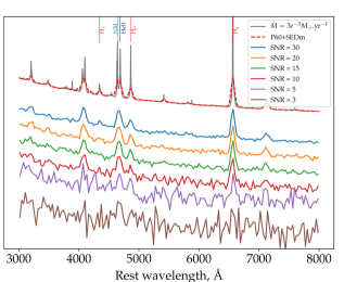
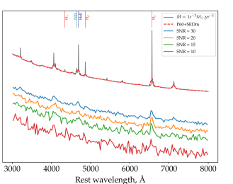
Figure 6: Simulating noisy SEDm spectra. Top: the strong flash-ionisation features template is used. With a SNR below 5, it is hard to detect even strong flash-ionisation features. Bottom: Weak flash ionisation template. Weak flash features can only be detected for a SNR above 15.

We used SEDm to obtain early spectra mainly due to its high availability and short response time. Being co-located with the survey telescope, we can obtain a spectrum $<1$ hour after we submit a trigger. However, due to the relatively small diameter of the telescope used (60”), the overall sensitivity of SEDm is limited. This makes it challenging to detect flash features in some spectra. For example, in Figure 7, we show a high resolution spectrum obtained with GMOS ($\mathcal{R}>1500$) and degrade it to the resolution of SEDm. Next, we change the SNR of the degraded spectrum to the measured SNR of a nearly contemporaneous SEDm spectrum. This shows that we cannot distinguish the flash lines (i.e. He II, and Balmer lines H$\alpha$ and H$\beta$) from the noisy continuum anymore. Hence if we had relied on a SEDm spectrum to identify flash features, this candidate would have been mislabeled as a non-flasher.
We examine the SNR of the ten non-flashers whose first spectrum was obtained with SEDm, see Table 3. In order to estimate a SNR threshold below which we cannot discriminate between flashers and non-flashers, we use the flash-spectra templates by Boian & Groh (2020) and degrade them to the resolution of SEDm and inject noise. We use templates with high mass-loss rate ($\dot{M}\approx 3\times 10^{-3}\,M_{\odot}$.yr^-1) to simulate strong flashers, and lower mass-loss rates ($\dot{M}\approx 1\times 10^{-3}\,M_{\odot}$.yr^-1) as weak flashers, see Figure 8. For weak flashers, a SNR $<15$ cannot be used to identify flash features. For strong flashers, a SNR $<5$ is unusable.

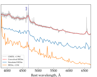
Figure 7: Simulation of an SEDm spectrum from a high-resolution GMOS spectrum, 2d after the estimated explosion. In blue is the simulated SEDm spectrum and in orange is a real SEDm spectrum obtained 3 days after estimated explosion time. Flash-ionisation features are visible in the GMOS spectrum. Once convolved to the SEDm resolution and noised, the flash features are indistinguishable from the noise. Without the GMOS spectrum, this candidate would have been classified as a non-flasher.

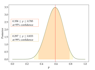
Figure 8: Posterior distribution of the probability for observing flash-features in the sample of candidates who had a first spectrum within less than 2 days from EED, having rejected candidates with a an SNR lower than 15 in their SEDm spectrum.

We eliminate seven events who have a SNR lower than 15,which leaves us with seventeen candidates, see Table 4. The spectra of the non flashers remaining in this sample can be found in Figure 9. The fraction of objects with CSM prior to explosion is then $58.8\%^{+19.7}_{-23}$, at 95% confidence interval (CI). In the unlikely case where we consider all flashers are strong flashers, only one candidate has a SNR lower than 5. In this case, the fraction lowers to $43.5\%^{+19.8}_{-17.9}$, at 95% CI (10 out of 23 have show flash features), see Figure 8. We conclude that it is likely that most progenitors of SNe II are embedded in CSM. These new results are consistent with our previously estimated fraction, Bruch et al. (2021).

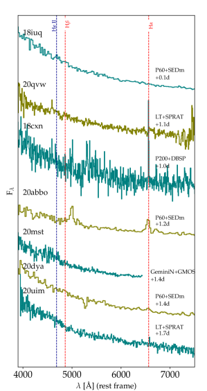
Figure 9: Spectra of the non-flashers from the 2-day subsample, excluding those which has a SNR lower than 15.

4.2 Comparison of the photometric properties of flashers and non-flasher events

Table 4: Subsample of SN II objects with a first spectrum within $<2$ d from EED. Objects with spectra whose SNR are below 15 were removed

IAU	Flasher	Time to	Telescope +	Redshift	Error on	Band	Peak Absolute	Error on	Rise	Error on
name		first spectrum	Instrument		redshift		magnitude	peak absolute	time	rise time
								magnitude
(SN)		[d]					[AB mag]	[AB mag]	[d]	[d]
2018iuq	no	0.11	SEDm+P60	0.026	0.0047	r	-18.60	0.39	12.18	1.30
						g	-18.75	0.39	11.51	0.39
2018grf	yes	0.14	SEDm+P60	0.054	0.0073	r	-18.52	0.30	6.29	0.39
						g	-18.58	0.30	4.88	0.29
2019nvm	yes	0.17	SEDm+P60	0.018	$<10^{-4}$	r	-17.64	0.01	8.58	0.57
						g	-17.47	0.02	7.68	1.22
2020qvw	no	0.71	SPRAT+LT	0.055	0.0028	r	-18.40	0.13	10.83	0.59
						g	-	-	-	-
2020pni	yes	0.86	DOLORES+TNG	0.017	$<10^{-4}$	r	-18.25	0.01	11.01	0.27
						g	-18.27	$<10^{-2}$	6.27	0.53
2020sic	yes	0.89	ALFOSC+NOT	0.033	0.0001	r	-17.87	0.29	12.37	1.57
						g	-	-	-	-
2018cxn	no	0.99	DBSP+P200	0.041	0.0001	r	-17.49	0.01	16.19	0.29
						g	-17.51	0.01	9.52	0.62
2018dfc	yes	1.02	SEDm+P60	0.037	0.0001	r	-18.50	0.02	10.43	1.50
						g	-18.55	0.01	7.37	1.35
2018fif	yes	1.13	DBSP+P200	0.017	$<10^{-4}$	r	-17.18	0.01	14.13	1.03
						g	-17.02	0.03	10.04	1.69
2020abbo	no	1.21	SEDm+P60	0.017	0.0012	r	-16.66	0.15	24.76	1.93
						g	-16.53	0.15	11.27	0.27
2020mst	no	1.30	GMOS+Gemini	0.058	0.0108	r	-18.13	0.41	15.06	0.72
						g	-18.09	0.41	10.90	0.84
2020dya	no	1.38	SEDm+P60	0.030	0.0001	r	-17.55	0.01	15.08	0.46
						g	-	-	-	-
2018cyg	yes?	1.68	ACAM+WHT	0.012	0.0002	r	-15.49	0.03	16.86	0.29
						g	-14.51	0.03	10.37	0.30
2020afdi	yes	1.69	DOLORES+TNG	0.024	0.0001	r	-15.88	0.01	6.26	0.92
						g	-15.94	0.01	4.72	0.55
2020uim	no	1.72	SPRAT+LT	0.018	0.0001	r	-16.78	0.02	18.62	1.46
						g	-16.87	0.02	7.19	0.73
2018egh	yes?	1.86	ISIS+WHT	0.038	0.0001	r	-16.81	0.01	16.74	0.78
						g	-16.66	0.03	5.72	0.60
2019ust	yes	1.99	GMOS+Gemini	0.022	$<10^{-4}$	r	-18.17	0.02	12.47	1.65
						g	-18.02	$<10^{-2}$	15.15	0.11

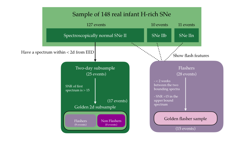
Figure 17: Schematic explanation of the subsamples used in this study. We use the golden 2-day subsample to compare the photometric parameters of flashers and non-flashers. We use the golden flasher sample to derive the durations of flash ionisation features

Strong CSM interaction may provide an additional power source, resulting usually in brighter events such as SNe IIn, see Smith (2016) and Nyholm et al. (2020). Since flash features also arise from CSM interaction, we want to test whether their early light curve behaviour differs from non-flashers. It was suggested that events showing flash features at early time would be brighter, see Hosseinzadeh et al. (2018).
In order to test this claim, we measure the peak absolute magnitude and rise time, as well as the color at peak in $g$ band of our sample, using the methods described earlier. We restrict our test to the subsample of normal SNe II for which we could robustly discriminate between flashers and non flashers, i.e. where we consider weak flashers (17 objects). We call this sub sample as the golden 2-day subsample, see Figure 17 in the Appendix.

We calculate the weighted mean of the peak absolute magnitude and rise time, and the standard deviation on the weighted mean. We find that flashers and non-flashers have almost identical peak magnitude distribution, see Fig. 10. Their mean values, M${}_{flash}=-18.02\pm 1.27$ mag and M${}_{noflash}=-18.10\pm 0.88$ mag in the $r$ band and M${}_{flash}=-17.90\pm 1.02$ mag and M${}_{noflash}=-18.08\pm 1.04$ mag in the $g$ band show that flashers are not brighter than non-flashers. A Kolmogorov-Smirnoff (KS) test reveals that the absolute peak magnitudes of flashers and non-flashers are not significantly different ($p_{value}=0.98$) in either of the bands (see Figure 11).
Flashers and non-flashers also have similar rise times (Figure 10), with flashers rising to peak in t${}^{g}_{rise}=7.81\pm 5.23$ days in the $g$ band and t${}^{r}_{rise}=11.62\pm 4.15$ days in the $r$ band compared to non-flashers : t${}^{g}_{rise}=9.77\pm 1.79$ days in the $g$ band and t${}^{r}_{rise}=17.73\pm 4.24$ days in the $r$ band. The KS test in the $g$ and $r$ band returns $p_{value,g}=0.30$ and $p_{value,r}=0.16$, respectively. As these values are higher than the threshold for a significant detection ($p=0.05$), we cannot reject the null hypothesis that these two distributions are drawn from the same parent distribution (see Figure 12).

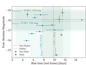
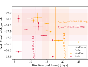
Figure 10: Peak absolute magnitude vs rise time for the 2d subsample in $g$ band (left) and $r$ band (right). The solid dark green (orange) lines indicate the weighted mean of the peak absolute magnitude (horizontal) and the weighted mean of the rise time (vertical) of non-flashers, the dashed teal (red) lines for flashers. The shaded area correspond to the corresponding weighted standard deviation.

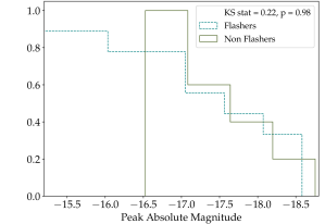
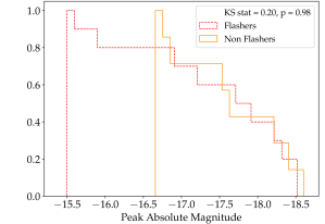
Figure 11: KS tests for the peak absolute magnitude distribution of flashers and non flashers in green (left) and red (right) bands.

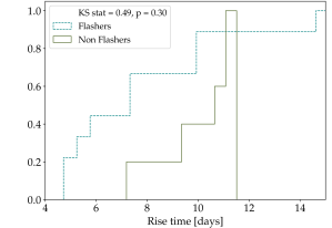
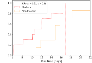
Figure 12: KS tests for the rise time distribution of flashers and non flashers in green (left) and red (right) bands.

We also investigate the color at the $g$ band peak . We use the interpolated light curves and subtract theirs values at peak g band. One candidate (SN2018cyg) has significant host extinction ($g-r$ = 0.9 mag). We had previously estimated the host extinction for this event using the method derived by Poznanski et al. (2012) and found that the absolute peak magnitude in the $g$ band is estimated to be extincted by nearly four magnitudes, see section 4.2 in Bruch et al. (2021). Excluding this object, the distribution in color at peak for flashers and non-flashers is similar. A KS test returns a p-value of 0.69, which indicates that the colors at peak in the $g$ band for flashers and non-flashers are also drawn from the same parent distribution.

At early time, SNe II with flash-ionisation features behave similarly to those without. This indicates that the CSM creating the flash features is not massive enough to contribute significantly to the luminosity of SNe II.

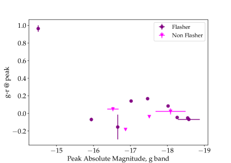
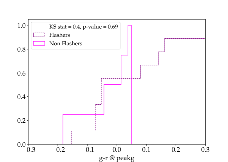
Figure 13: Top: color at peak of flasher (purple diamond) vs. non flasher (magenta triangle). Bottom: CDF of the two distributions, they are very likely to be drawn from the same distribution.

Table 5: Timescales of flash-ionisation features, peak absolute magnitudes in r band and g band.

IAU	Type	JD of	JD of	$\tau$	Error on	z	error	Band	Peak	$\delta$M	Rise	error on
name		last flash	no flash		$\tau$	z	on z		Abs. Mag		time	rise time
(SN)		[d]	[d]	[d]	[d]				[AB]	[AB]	[d]	[d]
2018grf	SN II	2458379.5	2458386.5	5.39	3.50	0.054	0.0073	r	-18.52	0.30	6.29	0.39
								g	-18.58	0.30	4.88	0.29
2019nvm	SN II	2458715.5	2458717.5	1.88	1.00	0.018	$<10^{-4}$	r	-17.64	0.01	8.58	0.57
								g	-17.47	0.02	7.68	1.22
2018dfi	SN IIb	2458307.5	2458311.5	2.25	2.05	0.031	0.0002	r	-17.61	0.01	2.66	0.43
								g	-17.76	0.02	1.72	0.44
2020pni	SN II	2459050.5	2459052.5	4.96	1.00	0.017	$<10^{-4}$	r	-18.25	0.01	11.01	0.27
								g	-18.27	$<10^{-2}$	6.27	0.53
2020sic	SN II	2459094.5	2459096.5	2.02	1.00	0.033	0.0001	r	-17.87	0.29	12.37	1.57
								g	-	-	-	-
2018dfc	SN II	2458307.5	2458312.5	6.23	2.83	0.037	0.0001	r	-18.50	0.02	10.43	1.50
								g	-18.55	0.01	7.37	1.35
2018fif	SN II	2458351.5	2458353.5	1.62	1.00	0.017	$<10^{-4}$	r	-17.18	0.01	14.13	1.03
								g	-17.02	0.03	10.04	1.69
2018cyg	SN II	2458295.5	2458296.5	1.28	0.50	0.012	0.0002	r	-15.49	0.03	16.86	0.29
								g	-14.51	0.03	10.37	0.30
2020afdi	SN II	2459071.5	2459072.5	1.30	0.50	0.024	0.0001	r	-15.88	0.01	6.26	0.92
								g	-15.94	0.01	4.72	0.55
2019ust	SN II	2458804.5	2458805.5	5.00	0.50	0.022	$<10^{-4}$	r	-18.17	0.02	12.47	1.65
								g	-18.02	$<10^{-2}$	15.15	0.11
2020lfn	SN II	2458998.5	2459001.5	4.18	1.50	0.044	0.0052	r	-18.95	0.26	10.80	0.63
								g	-18.96	0.26	9.13	0.29
2018cug	SN II	2458292.5	2458294.5	2.72	1.00	0.049	0.0024	r	-18.20	0.11	10.46	0.48
								g	-18.25	0.11	7.56	0.28
2020ufx	SN II	2459121.5	2459123.5	4.88	1.00	0.051	0.0021	r	-18.93	0.09	10.84	0.70
								g	-19.14	0.09	6.11	0.45
2020pqv	SN II	2459049.5	2459054.5	5.21	2.51	0.034	$<10^{-4}$	r	-18.02	0.01	24.65	0.87
								g	-17.72	$<10^{-2}$	4.56	0.16
2018leh	SN II	2458484.5	2458486.5	7.59	5.50	0.024	$<10^{-4}$	r	-18.01	0.01	14.70	0.15
								g	-18.05	$<10^{-2}$	12.49	0.14
2020wol	SN II	2459143.5	2459156.5	13.56	6.51	0.050	0.0100	r	-18.92	0.43	16.25	0.77
								g	-19.05	0.43	10.97	0.64
2019qch	SN II	2458750.5	2458751.5	14.64	1.13	0.024	0.0014	r	-18.23	0.13	19.74	1.03
								g	-18.40	0.13	15.67	1.04
2019mor	SN II	2458699.5	2458703.5	8.28	2.50	0.019	0.0001	r	-17.18	0.02	12.97	1.53
								g	-17.35	0.01	11.49	1.50
2019lkw	SN II	2458690.5	2458696.5	17.15	3.10	0.073	0.0021	r	-20.13	0.06	14.03	0.83
								g	-20.37	0.06	13.37	0.81

4.3 Duration of flash features

We estimate the flash timescale as the time from the estimated explosion date until the half-time between the last spectrum still showing a He II (4686Å) line and the first spectrum not showing He II line anymore, see Table 5. We designate these two spectra as bounding spectra. We look for correlations of flash-feature timescales against peak absolute magnitude and rise time, considering all the infant candidates which showed flash-features and from which we could estimate a timescale (15 out of 29). We disqualify those for which the time between the last spectrum showing the He II emission line and the first with no line or broad feature was longer than 14 days. We also disqualify candidates whose first spectrum with no He II line had a SNR lower than 15. We designate this subsample as the golden flasher sample, see Figure 17 in the Appendix.

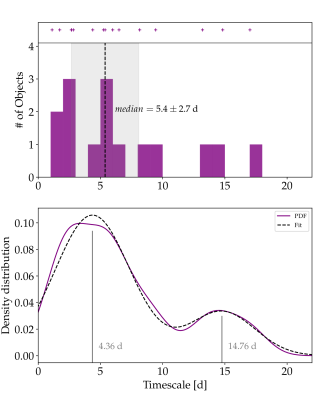
Figure 14: Histogram of the timescales for flash ionisation features over a sample of 15 candidates.

The distribution of flash timescales (Fig. 14) shows that most SNe have a characteristic timescale of flash features shorter than $5.4\pm 2.7$ days. We extract the probability distribution function of the timescale of flash features, using Kernel Density estimation. We represent each measurement as a Gaussian kernel function, whose mean is the value of the measurement. We chose a fixed-width kernel. The width is the median value of all the estimated errors, i.e. $\sigma=1.48$d. The resulting estimated density is the bottom panel in Figure 14. We fit two Gaussians and find two clusters at 4.36 d and 14.76 d respectively. The size of our sample is however too small to interpret this probability density function (PDF) meaningfully. While a single Gaussian cannot reproduce the timescale measurements at $\geq 12$ days, it is not yet possible to tell whether the longer-lived flasher belong to a distinct family (which would show different physical properties in interaction with the CSM); or if the PDF is a skewed normal distribution, hence making longer-lived flasher a rarer population.

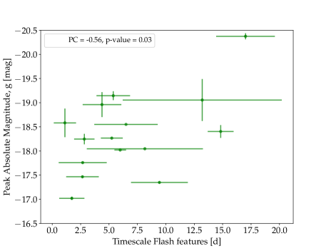
Figure 15: Flash timescale vs. peak magnitude

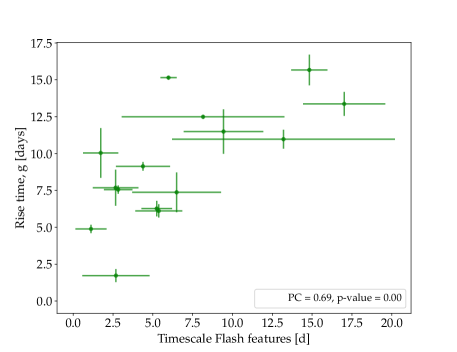
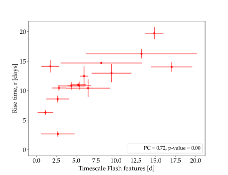
Figure 16: Flash timescale vs. rise time

We find a partial correlation between the flash features time scale and the peak absolute magnitude: the Pearson correlation coefficient is $-0.51$ in $r$ band and $-0.56$ in $g$ band, see Fig 15. The probability for an uncorrelated distribution to generate such a coefficient is low, with a p-value of $\lesssim 0.05$. However, it seems that the long-lived flasher population, with timescales longer than 10 days, are driving this correlation. The low number of observations in our sample does not allow us to make any strong conclusion. The flash feature timescale is correlated with the rise time, with a Pearson coefficient of 0.69 in the $g$ band and 0.72 in the $r$ band. The p-values in both cases are $\lesssim 0.05$, hence excluding the chance that an uncorrelated distribution could generate such coefficient. We observe that the longer the flash timescale is, the longer the rise time is to a brighter peak.

Our work suggests, for the first time, that there exist a characteristic timescale which may separate events where the CSM does not significantly influence the brightness of the light curve ($<9$ days, common flashers), and events where the CSM does ($>9$ days, long-lived flash features). In the latter case, such events display brighter peaks and a slower rise to the peak. This population of long-lasting flashers could be considered as the low-CSM mass tail of the population of SNe IIn.

5 Conclusion

We report the results of the search for flash-ionisation features in infant, hydrogen-rich SNe during the first phase of ZTF (from March 2018 to December 2020). We collected 148 such objects (at a rate of once to twice a week) and obtained rapid follow-up spectroscopy within $2$ d from estimated explosion for 25 of the SNe classified as spectroscopically-normal SNe II.
Fast response spectroscopic facilities were essential, such as the SEDm with which we obtained 13 of those spectra. However, 7 were disqualified due to their low S/N ratio. We corroborated our previous results, see Bruch et al. (2021), that flash-ionisation features occur in at least 30%, and likely most, hydrogen-rich SNe. This implies that a confined CSM is common around hydrogen-rich SN progenitors.
We also investigated the early light-curve behaviour (i.e. rise times, peak magnitudes and color at peak) of 17 events which have a spectrum less than two days from estimated explosion. We find that there is no significant difference between candidates showing flash-ionisation features and those who do not at early time. We hence conclude that the confined CSM of most SNe is not massive enough to contribute extra energy to the light curve at early time.
We present for the first time a sample of flash ionisation events with sequences measuring the timescale of disappearance of flash-ionisation features. Typical flash events last for $\approx 5$ days. A rarer population of flashers have timescales above $10$ days from the estimated explosion time. This population have longer rise times and reach brighter peak magnitudes. We hypothesize that this group bridges between spectroscopically-normal SNe II and strongly interacting SNe IIn. It is not clear yet if the distribution of timescale of flash-ionisation features is bimodal (i.e. two distinct population of typical flashers and long-lasting flashers) or a skewed normal distribution (i.e. long lasting flashers are just rarer). Our results also question the CSM properties as well as the regime of CSM interaction in which flash feature are.
Since no significant rise time or peak absolute magnitude difference is found between events with flash features and those without, we could hypothesize that no significant energy conversion is taking place between the ejecta and the CSM. Thus making the regime of interaction for common flash ionisation shockless. Events for which higher peak magnitudes and longer rise times are recorded could thus also represent a transitional population from flash ionisation to shock ionisation. These different regimes of interaction would be a direct consequence of the CSM properties, i.e. from optically thin and confined for regular flash ionisation to optically thick and extended for shock ionisation.
Our results motivate the systematic acquisition of series of spectra for young, hydrogen-rich SNe. While we have established that the presence of CSM is common around massive star progenitors, the properties of the CSM, such as density profile, composition, compactness were not studied over big samples. Mapping these properties will shed light on the environment and circumstances prior to the explosion of hydrogen-rich SN progenitors. Such studies are currently ongoing in partnership with the ePessto$+$ survey, using the EFOSC2 (R$\approx 390$) on the NTT spectrographs. They should be continued with the upcoming instrument SoXs, a mid-resolution spectrograph (R$\approx 4500$) with high throughput Rubin et al. (2020). This instrument will be dedicated to transient science with Target of Opportunity observing strategy, hence allowing for more systematic rapid-response spectroscopic follow up. The commissioning of SoXs is planned to start in September 2023.

Appendix A The hydrogen rich sample

Table 6: Hydrogen rich normal SNe II (part 1/3)

IAU	ZTF	Type	Explosion	Error	Last	First	RA	DEC	First	Flasher
name	name		JD date		Non	detection	(median)	(median)	spectrum
	(ZTF)				detection
			[d]	[d]	[d]	[d]	[degrees]	[degrees]	[d]
2018iuq	18acqwdla	SN II	2458443.832	0.042	-0.043	0.042	106.472662	12.8929375	0.105	no
2018grf	18abwlsoi	SN II	2458377.609	0.003	-0.869	0.021	261.897614	71.530251	0.142	yes
2020acbm	20acwgxhk	SN II	2459193.562	0.030	-0.850	0.125	40.0741593	2.4270671	0.167	no
2019nvm	19abqhobb	SN II	2458714.625	0.006	-0.883	0.038	261.4111	59.4467303	0.167	yes
2020qvw	20abqkaoc	SN II	2459067.290	0.490	-0.490	0.490	250.983335	77.879897	0.710	no
2020pni	20ablygyy	SN II	2459046.539	0.031	-0.785	0.159	225.958184	42.1140315	0.864	yes
2020sic	20abxyjtx	SN II	2459093.484	0.008	-1.768	0.150	236.937978	28.6403193	0.891	yes
2018cxn	18abckutn	SN II	2458289.758	0.015	0.000	0.107	237.026897	55.7148553	0.990	no
2018dfc	18abeajml	SN II	2458303.773	1.332	-0.976	0.026	252.03236	24.3040949	1.021	yes
2019omp	19abrlvij	SN II	2458718.809	0.010	0.001	0.841	260.142987	51.6327799	1.054	no
2019ewb	19aatqzrb	SN II	2458606.787	0.003	-0.899	0.012	221.652383	56.2342197	1.083	no
2020dyu	20aasfhia	SN II	2458912.697	0.012	-0.727	0.083	184.913045	33.0403926	1.121	no
2018fif	18abokyfk	SN II	2458350.877	0.008	-0.976	0.013	2.360629	47.3540827	1.129	yes
2020abbo	20acuaqlf	SN II	2459181.374	0.060	-1.703	0.234	357.775211	6.9424927	1.206	no
2020mst	20abfcdkj	SN II	2459013.701	0.008	-0.881	0.049	281.793965	60.4968018	1.299	no
2020dya	20aasijew	SN II	2458912.504	0.454	-0.454	0.454	216.905399	69.6864096	1.379	no
2020sjv	20abybeex	SN II	2459094.200	0.498	-0.499	0.498	260.769541	55.0724721	1.508	no
2018cyg	18abdbysy	SN II	2458294.724	0.002	0.057	0.981	233.535367	56.6968577	1.676	yes?
2020afdi	20abqwkxs	SN II	2459070.698	0.029	-0.899	0.006	224.868111	73.8986784	1.693	yes
2020uim	20acfdmex	SN II	2459118.846	0.005	-0.985	0.002	28.1887405	36.6231594	1.719	no
2018egh	18abgqvwv	SN II	2458312.710	0.001	0.128	1.020	254.316401	31.9631992	1.859	yes?
2020xhs	20acknpig	SN II	2459139.073	0.059	-0.206	1.685	30.7428678	45.0202856	1.888	no
2019ikb	19abbwfgp	SN II	2458661.817	3.554	-0.974	0.003	258.323795	43.7843194	1.942	no
2019ust	19acryurj	SN II	2458799.997	0.032	-0.192	0.793	13.5933959	31.6701819	1.994	yes
2020lfn	20abccixp	SN II	2458995.816	0.002	0.004	0.954	246.737034	20.2459056	2.011	yes
2019dky	19aapygmq	SN II	2458584.778	4.036	0.093	0.978	210.421485	38.5103291	2.047	no
2019odf	19abqrhvy	SN II	2458714.844	0.008	0.028	1.073	342.186213	27.5718269	2.139	no
2019gmh	19aawgxdn	SN II	2458633.768	5.618	0.078	1.940	247.763189	41.1539613	2.166	yes?
2018bqs	18aarpttw	SN II	2458246.812	0.001	-1.963	0.010	247.259916	43.6268251	2.188	no
2020uhf	20aceyolc	SN II	2459118.795	0.004	-0.903	0.001	44.102817	38.1871607	2.205	yes
2018cug	18abcptmt	SN II	2458290.779	0.022	-0.038	0.085	267.329908	49.412409	2.221	yes
2019oxn	19abueupg	SN II	2458724.584	0.012	-0.774	0.066	267.80329	51.3825496	2.281	no
2019szo	19acgbkzr	SN II	2458775.334	0.012	-0.619	0.471	4.9860264	15.0933857	2.282	no
2020ufx	20acedqis	SN II	2459117.623	0.010	-0.784	0.020	322.652706	24.6737523	2.377	yes
2020umi	20acfkzcg	SN II	2459119.496	0.477	-0.478	0.477	115.76978	50.2887543	2.413	no
2019dlo	19aapvltt	SN II	2458583.799	0.101	-0.810	0.087	267.6325156	58.6245046	2.701	no
2018fsm	18absldfl	SN II	2458362.965	0.009	0.005	0.915	33.5997569	30.811935	2.825	no

Table 7: Hydrogen rich normal SNe II (part 2/3)

IAU	ZTF	Type	Explosion	Error	Last	First	RA	DEC	First	Flasher
name	name		JD date		Non	detection	(median)	(median)	spectrum
	(ZTF)				detection
			[d]	[d]	[d]	[d]	[degrees]	[degrees]	[d]
2020zpt	20acqexmr	SN II	2459166.900	0.025	-1.966	0.014	57.9034378	43.6980162	2.828	no
2020xva	20aclvtnk	SN II	2459141.653	2.184	1.965	1.989	263.035128	53.6539888	2.847	no
2018gts	18abvvmdf	SN II	2458373.738	0.003	0.000	0.896	249.197462	55.7357948	2.881	yes
2018bge	18aaqkoyr	SN II	2458242.776	0.198	-0.126	0.909	166.066683	50.0306395	2.908	no
2020uao	20accrldu	SN II	2459114.783	0.004	-0.893	0.041	17.1983968	27.0450181	2.912	no
2020yui	18aadsuxd	SN II	2459154.018	0.007	0.000	1.947	129.533971	31.667916	2.921	no
2019eoh	19aatqzim	SN II	2458604.976	0.422	-3.194	1.715	195.955635	38.2891552	2.930	no
2020ifv	20aawgrcu	SN II	2458963.957	0.024	-0.007	0.943	310.650913	76.7817657	2.939	no
2020pqv	20abmoakx	SN II	2459046.791	0.164	-0.081	1.968	220.49818	8.46272355	2.989	yes
2018leh	18adbmrug	SN II	2458482.405	0.039	-1.603	0.294	61.2637726	25.2619268	3.044	yes
2020uqx	20acgided	SN II	2459123.544	0.049	-0.800	0.153	326.826979	32.0957996	3.143	yes
2020wol	20acjbhhp	SN II	2459136.445	0.291	-1.615	0.385	29.8613506	30.726751	3.240	yes
2020dbg	20aapycrh	SN II	2458900.752	0.056	-0.884	0.007	164.245241	43.0768461	3.248	no
2019twk	19aclobbu	SN II	2458788.242	0.087	-1.482	0.528	35.7720108	46.8824189	3.407	no
2020wog	20aciwrpn	SN II	2459135.971	0.067	-1.251	0.689	328.182556	33.6561827	3.797	no
2020ykb	20acocohy	SN II	2459149.954	0.042	-0.012	0.943	64.0382399	-25.474303	3.865	no
2020iez	20aavvaup	SN II	2458962.615	0.007	-7.898	0.065	147.118273	50.9224955	3.885	no
2019ssi	19acftfav	SN II	2458773.704	0.053	0.048	0.993	352.733873	15.4916278	3.890	no
2020sje	20abxmwwd	SN II	2459089.911	0.041	0.049	0.959	19.3414942	44.1948692	3.963	no
2020dbd	20aapjiwl	SN II	2458899.750	0.027	-0.940	0.011	142.988659	33.2096657	4.125	no
2019lnl	19abgrmfu	SN II	2458681.566	0.020	-0.811	0.117	255.526652	32.9977641	4.154	no
2020iyi	20aaxunbm	SN II	2458969.452	0.045	-0.712	0.231	152.764995	54.369596	4.233	no
2018iua	18acploez	SN II	2458439.478	0.469	-0.469	0.468	130.037293	68.9031911	4.303	no
2020ovk	20ablklei	SN II	2459042.418	0.024	-1.433	0.443	358.573861	26.3267084	4.472	no
2020cvy	20aaophpu	SN II	2458895.697	0.030	1.026	2.993	120.205292	27.4985715	4.943	no
2020ult	20acfkyll	SN II	2459119.496	0.477	-0.478	0.477	106.885226	48.9002151	5.160	no
2020rjd	20absgwch	SN II	2459075.643	0.033	-1.735	0.265	359.74376	3.7404556	5.214	no?
2020yts	20acongti	SN II	2459153.623	0.002	0.116	1.068	338.614616	25.0352627	5.223	no
2019tjt	19acignlo	SN II	2458782.626	2.238	-0.966	0.004	4.2653086	31.5725235	5.374	yes
2020rth	20abupxie	SN II	2459080.475	0.485	-0.485	0.485	52.1135451	-5.2545457	5.525	no
2018fpb	18abqyvzy	SN II	2458357.826	0.005	-0.856	0.089	359.9284	34.3444464	5.873	no
2020dbn	20aaqbach	SN II	2458899.926	0.009	0.068	0.911	187.036133	20.178184	5.990	no
2018gvn	18abyvenk	SN II	2458385.618	0.509	-0.858	0.002	273.976407	44.6964598	6.114	no
2019oba	19abpyqog	SN II	2458711.672	0.003	-0.824	1.079	299.264485	50.1889432	6.129	no
2020pnn	20abmihnc	SN II	2459044.747	0.026	-2.955	0.000	271.019773	22.0370976	6.193	no
2019qch	19abyuzch	SN II	2458736.360	1.017	2.281	3.280	277.30754	41.0423427	6.265	yes
2019cem	19aamtwiz	SN II	2458559.435	0.083	-0.581	0.334	199.151274	35.516058	6.345	no
2018clq	18aatlfus	SN II	2458248.900	0.958	-0.959	0.958	257.176414	28.5206041	6.925	no
2019mor	19abjsmmv	SN II	2458693.223	1.500	-1.500	1.500	234.658542	36.9586362	7.439	yes
2019vdl	19actnwtn	SN II	2458804.018	0.972	-0.972	0.971	142.38251	44.4222435	7.857	no
2019oot	19abrbmvt	SN II	2458716.891	0.004	-0.004	0.004	345.069535	24.7855163	8.014	no
2020jmb	20aayrobw	SN II	2458977.190	0.470	-0.470	0.470	142.804994	38.2540186	8.810	no

Table 8: Hydrogen rich normal SNe II (part 3/3)

IAU	ZTF	Type	Explosion	Error	Last	First	RA	DEC	First	Flasher
name	name		JD date		Non	detection	(median)	(median)	spectrum
	(ZTF)				detection
			[d]	[d]	[d]	[d]	[degrees]	[degrees]	[d]
2019tbq	19acgzzea	SN II	2458776.871	0.152	-0.939	0.062	77.9474245	52.5389439	8.845	no
2018inm	18achtnvk	SN II	2458432.878	2.559	0.073	1.983	96.1686908	46.5038794	9.047	no
2018ccp	18aawyjjq	SN II	2458262.857	0.024	-0.910	0.049	263.058847	36.0739975	9.143	no
2019rsw	19accbeju	SN II	2458757.761	0.037	-0.847	0.174	37.8938775	24.8167672	9.164	no
2020iho	20aawbzlo	SN II	2458964.616	0.020	-0.862	0.082	166.411236	30.8325541	9.191	no
2019lkw	19abgpgyp	SN II	2458676.348	0.790	0.475	1.420	256.287926	33.4425697	9.544	yes
2020jww	20aazpphd	SN II	2458982.874	1.077	-1.077	1.076	242.714935	27.1616704	9.988	no
2018lth	18aayxxew	SN II	2458276.725	0.007	0.015	1.975	197.139654	45.9862178	10.091	no
2020buc	18aaaibml	SN II	2458881.397	0.475	-0.476	0.475	152.130328	9.2397339	10.118	yes
2019mge	19abjioie	SN II	2458691.398	0.213	0.410	1.310	259.203094	39.1480677	11.405	yes
2018iwe	18abufaej	SN II	2458368.807	0.002	-0.906	0.001	4.4825224	12.091568	12.065	no
2020lam	20abbpkpa	SN II	2458992.833	2.776	0.000	2.082	254.098077	26.8138571	12.112	no
2019mkr	19abjrjdw	SN II	2458694.510	0.044	-1.792	0.167	257.774102	5.8520255	12.200	no
2020rhg	20abqferm	SN II	2459065.415	0.505	-0.505	0.505	9.7067662	3.4036991	12.494	no
2018iug	18acnmifq	SN II	2458437.855	0.040	-1.022	0.013	101.979329	67.9163152	12.834	no
2020smm	20abykfsr	SN II	2459094.835	0.005	0.055	1.092	60.9976329	28.6198327	13.162	no
2018egj	18abeewyu	SN II	2458303.653	0.308	-0.943	0.157	250.955014	47.4085778	13.347	no
2019wvz	19acytcsg	SN II	2458831.951	0.005	0.102	1.986	155.119472	50.4679327	13.827	no
2018fso	18abrlljc	SN II	2458357.603	0.005	-0.820	0.078	253.184108	70.0882348	14.107	no
2019kes	19abegizf	SN II	2458665.452	2.483	-2.484	2.483	328.034016	-23.364074	15.373	no
2020aasd	20actawpa	SN II	2459175.306	0.437	0.604	0.714	140.812575	33.5669093	15.694	no
2020sur	20abywoaa	SN II	2459092.390	0.510	-0.510	0.510	22.2482141	-11.491487	16.537	no
2020rid	20abpwdfd	SN II	2459060.662	4.501	0.017	2.001	181.833961	57.6346927	16.729	no
2018mbn	18abgxjie	SN II	2458312.713	0.048	0.220	1.004	285.008531	51.9231897	17.981	no
2019hln	19aaymhay	SN II	2458642.772	0.011	-0.805	0.010	287.957064	50.8476251	18.058	no
2018cyh	18abcezmh	SN II	2458284.848	2.120	0.035	0.964	269.451874	40.0763824	18.152	no
2019fkl	19aavbjfp	SN II	2458617.228	0.478	-0.479	0.478	186.753673	62.1638376	18.569	no
2020lcc	20abbeoaa	SN II	2458991.762	0.004	-5.973	0.030	231.265297	8.4907814	18.738	no
2018bdv	18aapifti	SN II	2458230.834	0.002	0.853	2.844	177.017646	30.3600716	18.883	no
2019fmv	19aavbkly	SN II	2458618.236	0.481	-0.481	0.480	187.390843	35.7700404	20.564	no
2020oco	20abjuxoy	SN II	2459025.703	0.836	4.057	5.187	292.040677	52.8939923	22.092	no
2018dzo	18abeteea	SN II	2458303.683	0.050	-0.843	0.027	230.63751	36.7986147	22.317	no
2019pkh	19abuzinv	SN II	2458726.450	0.520	-0.520	0.520	34.8642701	34.0819977	22.550	no
2020ttu	20acaiztt	SN II	2459109.845	0.023	-1.905	0.005	41.8004692	41.4099111	25.270	no
2019jhe	19aaxqwjx	SN II	2458639.712	0.002	-0.001	0.045	236.891446	33.5519041	26.142	no
2020umb	20acedspv	SN II	2459116.625	0.090	-0.875	0.125	336.870395	12.4784784	27.250	no
2019aaqx	19abmxtrm	SN II	2458696.792	0.015	-0.015	0.014	243.546215	59.0099127	32.209	no
2018bjh	18aahrzrb	SN II	2458217.581	0.044	-0.841	0.159	181.397225	34.3888042	34.236	no
2020drl	20aarbvub	SN II	2458905.178	0.478	-0.478	0.478	112.047976	72.5781035	34.456	no
2020yyo	20acpevli	SN II	2459157.715	0.002	-0.682	0.197	167.480755	79.0043096	36.939	no
2018lti	18abddjpt	SN II	2458294.706	0.036	-0.876	0.085	278.704811	38.2987135	40.294	no
2018efj	18abimhfu	SN II	2458320.653	0.002	-0.903	0.017	240.142272	31.6429506	42.014	no
2018mdz	18abcqhgr	SN II	2458290.743	0.389	0.119	1.041	254.818204	60.4317906	46.105	no
2020ks	20aaczkyw	SN II	2458850.736	0.045	-0.761	0.236	84.6766286	81.2087595	54.264	no
2018cfj	18aavpady	SN II	2458256.114	0.107	-0.138	0.816	273.003116	44.3601877	55.886	no
2020sfy	20abwftit	SN II	2459085.460	0.480	-0.480	0.480	33.103797	-12.375219	58.527	no
2018mdx	18aaxwrjt	SN II	2458273.777	0.007	-0.837	0.013	260.363393	25.6504719	70.223	no
2020pvg	20abojbrd	SN II	2459049.396	0.496	-0.497	0.496	342.184072	-19.829618	94.456	no

Table 9: Real infants classified as SN IIn

IAU	ZTF	Type	Explosion	Error	Last	First	RA	DEC	First	Flasher
name	name		JD date		Non	detection	(median)	(median)	spectrum
	(ZTF)				detection
			[d]	[d]	[d]	[d]	[degrees]	[degrees]	[d]
2019njv	ZTF19abpidqn	SN IIn	2458707.708	0.067	-0.816	0.005	304.988297	15.3774528	1.150	no
2020dcs	ZTF20aaocqkr	SN IIn	2458895.153	0.032	-0.168	0.778	183.356159	37.6993902	2.484	yes
2020rfs	ZTF20abrmbdl	SN IIn	2459072.375	0.445	-0.445	0.445	282.303159	74.3340239	3.125	no
2020xkx	ZTF20acklcyp	SN IIn	2459137.743	1.008	-1.008	1.007	350.11738	22.9869004	7.870	no
2019smj	ZTF19aceqlxc	SN IIn	2458767.998	0.970	-0.970	0.969	117.419661	5.0742059	11.899	no
2019dvw	ZTF19aapafqd	SN IIn	2458571.416	1.512	-1.513	1.512	239.944168	37.033706	15.539	no
2019pgu	ZTF19abulzhy	SN IIn	2458722.562	0.077	0.235	1.234	244.678475	67.9000902	18.120	no
2020cnv	ZTF20aahapgw	SN IIn	2458861.167	0.503	-0.504	0.503	62.6199901	34.112782	30.834	no
2018gfx	ZTF18abtswjk	SN IIn	2458366.563	0.212	-0.567	0.384	38.2980122	-1.3056566	31.380	no
2018dfa	ZTF18abcfdzu	SN IIn	2458286.576	0.214	-0.770	0.152	230.217161	54.2155543	32.424	no
2019pdm	ZTF19abmouqp	SN IIn	2458693.887	0.028	1.071	2.020	353.667326	16.4185618	39.113	no

Table 10: Real infants classified as SN IIb

IAU	ZTF	Type	Explosion	Error	Last	First	RA	DEC	First	Flasher
name	name		JD date		Non	detection	(median)	(median)	spectrum
	(ZTF)				detection
			[d]	[d]	[d]	[d]	[degrees]	[degrees]	[d]
2020sbw	ZTF20abwzqzo	SN IIb	2459087.465	0.482	-0.482	0.482	41.5138221	3.329908	0.578	no
2018dfi	ZTF18abffyqp	SN IIb	2458307.254	0.432	-0.432	0.432	252.708677	45.3978958	0.596	yes
2018fzn	ZTF18abojpnr	SN IIb	2458350.935	0.003	-0.001	0.724	297.487196	59.5927746	0.962	no
2019dwf	ZTF19aarfkch	SN IIb	2458592.665	0.013	-0.745	0.015	221.131644	70.4559895	1.183	no
2019ehk	ZTF19aatesgp	SN IIb	2458602.285	0.500	-0.500	0.500	185.733956	15.826127	1.474	yes
2019rwd	ZTF19acctwpz	SN IIb	2458761.165	0.485	-0.485	0.485	2.691207	21.1390942	1.568	no
2020urc	ZTF20acgiglu	SN IIb	2459123.366	0.474	-0.475	0.474	34.5461651	37.0971887	2.341	no
2018mdy	ZTF18aaymsbe	SN IIb	2458276.640	0.005	-1.756	0.166	243.77589	62.3191198	9.360	no
2018jak	ZTF18acqxyiq	SN IIb	2458442.985	0.960	-0.960	0.959	149.825817	34.8954985	14.033	no
2018efd	ZTF18abgrbjb	SN IIb	2458312.867	0.005	0.066	0.850	274.998606	51.7964817	14.964	no

References

- Bellm & Sesar (2016) Bellm, E. C., & Sesar, B. 2016, pyraf-dbsp: Reduction pipeline for the Palomar Double Beam Spectrograph. http://ascl.net/1602.002
- Bellm et al. (2019) Bellm, E. C., Kulkarni, S. R., Graham, M. J., et al. 2019, PASP, 131, 018002, doi: 10.1088/1538-3873/aaecbe
- Ben-Ami et al. (2012) Ben-Ami, S., Konidaris, N., Quimby, R., et al. 2012, in Society of Photo-Optical Instrumentation Engineers (SPIE) Conference Series, Vol. 8446, Proc. SPIE, 844686, doi: 10.1117/12.926317
- Benn et al. (2008) Benn, C., Dee, K., & Agócs, T. 2008, in Society of Photo-Optical Instrumentation Engineers (SPIE) Conference Series, Vol. 7014, Proc. SPIE, 70146X, doi: 10.1117/12.788694
- Blagorodnova et al. (2018) Blagorodnova, N., Neill, J. D., Walters, R., et al. 2018, PASP, 130, 035003, doi: 10.1088/1538-3873/aaa53f
- Boian & Groh (2020) Boian, I., & Groh, J. H. 2020, MNRAS, 496, 1325, doi: 10.1093/mnras/staa1540
- Bruch et al. (2021) Bruch, R. J., Gal-Yam, A., Schulze, S., et al. 2021, ApJ, 912, 46, doi: 10.3847/1538-4357/abef05
- Cenko et al. (2006) Cenko, S. B., Fox, D. B., Moon, D.-S., et al. 2006, PASP, 118, 1396, doi: 10.1086/508366
- Chugai & Danziger (1994) Chugai, N. N., & Danziger, I. J. 1994, MNRAS, 268, 173, doi: 10.1093/mnras/268.1.173
- Davenport (2018) Davenport. 2018, pyDIS, doi, doi: doi:10.5281/zenodo.58753
- Dekany et al. (2020) Dekany, R., Smith, R. M., Riddle, R., et al. 2020, PASP, 132, 038001, doi: 10.1088/1538-3873/ab4ca2
- Dembinski et al. (2020) Dembinski, H., Ongmongkolkul, P., Deil, C., et al. 2020, scikit-hep/iminuit: v2.2.1, v2.2.1, Zenodo, doi: 10.5281/zenodo.4386859
- Filippenko (1997) Filippenko, A. V. 1997, ARA&A, 35, 309, doi: 10.1146/annurev.astro.35.1.309
- Gal-Yam (2017) Gal-Yam, A. 2017, Observational and Physical Classification of Supernovae, ed. A. W. Alsabti & P. Murdin, 195, doi: 10.1007/978-3-319-21846-5_35
- Gal-Yam et al. (2011) Gal-Yam, A., Kasliwal, M. M., Arcavi, I., et al. 2011, ApJ, 736, 159, doi: 10.1088/0004-637X/736/2/159
- Gal-Yam et al. (2014) Gal-Yam, A., Arcavi, I., Ofek, E. O., et al. 2014, Nature, 509, 471, doi: 10.1038/nature13304
- Goldoni et al. (2006) Goldoni, P., Royer, F., François, P., et al. 2006, in Society of Photo-Optical Instrumentation Engineers (SPIE) Conference Series, Vol. 6269, Society of Photo-Optical Instrumentation Engineers (SPIE) Conference Series, ed. I. S. McLean & M. Iye, 62692K, doi: 10.1117/12.669986
- Graham et al. (2019) Graham, M. J., Kulkarni, S. R., Bellm, E. C., et al. 2019, PASP, 131, 078001, doi: 10.1088/1538-3873/ab006c
- Hook et al. (2004) Hook, I. M., Jørgensen, I., Allington-Smith, J. R., et al. 2004, PASP, 116, 425, doi: 10.1086/383624
- Hosseinzadeh et al. (2018) Hosseinzadeh, G., Valenti, S., McCully, C., et al. 2018, ApJ, 861, 63, doi: 10.3847/1538-4357/aac5f6
- Jacobson-Galán et al. (2022) Jacobson-Galán, W. V., Dessart, L., Jones, D. O., et al. 2022, ApJ, 924, 15, doi: 10.3847/1538-4357/ac3f3a
- Jóhannesson et al. (2006) Jóhannesson, G., Björnsson, G., & Gudmundsson, E. H. 2006, ApJ, 640, L5, doi: 10.1086/503294
- Kasliwal et al. (2019) Kasliwal, M. M., Cannella, C., Bagdasaryan, A., et al. 2019, PASP, 131, 038003, doi: 10.1088/1538-3873/aafbc2
- Khazov et al. (2016) Khazov, D., Yaron, O., Gal-Yam, A., et al. 2016, ApJ, 818, 3, doi: 10.3847/0004-637X/818/1/3
- Kiewe et al. (2012) Kiewe, M., Gal-Yam, A., Arcavi, I., et al. 2012, ApJ, 744, 10, doi: 10.1088/0004-637X/744/1/10
- Kim et al. (2022) Kim, Y. L., Rigault, M., Neill, J. D., et al. 2022, PASP, 134, 024505, doi: 10.1088/1538-3873/ac50a0
- Meakin & Arnett (2007) Meakin, C. A., & Arnett, D. 2007, ApJ, 665, 690, doi: 10.1086/519372
- Modigliani et al. (2010) Modigliani, A., Goldoni, P., Royer, F., et al. 2010, in Society of Photo-Optical Instrumentation Engineers (SPIE) Conference Series, Vol. 7737, Observatory Operations: Strategies, Processes, and Systems III, ed. D. R. Silva, A. B. Peck, & B. T. Soifer, 773728, doi: 10.1117/12.857211
- Morozova et al. (2017) Morozova, V., Piro, A. L., & Valenti, S. 2017, ApJ, 838, 28, doi: 10.3847/1538-4357/aa6251
- Neill (2019) Neill, J. D. 2019, in The Extragalactic Explosive Universe: the New Era of Transient Surveys and Data-Driven Discovery, 38, doi: 10.5281/zenodo.3478070
- Niemela et al. (1985) Niemela, V. S., Ruiz, M. T., & Phillips, M. M. 1985, ApJ, 289, 52, doi: 10.1086/162863
- Nordin et al. (2019) Nordin, J., Brinnel, V., van Santen, J., et al. 2019, A&A, 631, A147, doi: 10.1051/0004-6361/201935634
- Nyholm et al. (2020) Nyholm, A., Sollerman, J., Tartaglia, L., et al. 2020, A&A, 637, A73, doi: 10.1051/0004-6361/201936097
- Ochsenbein et al. (2000) Ochsenbein, F., Bauer, P., & Marcout, J. 2000, A&AS, 143, 23, doi: 10.1051/aas:2000169
- Ofek et al. (2013) Ofek, E. O., Sullivan, M., Cenko, S. B., et al. 2013, Nature, 494, 65, doi: 10.1038/nature11877
- Ofek et al. (2014) Ofek, E. O., Sullivan, M., Shaviv, N. J., et al. 2014, ApJ, 789, 104, doi: 10.1088/0004-637X/789/2/104
- Oke & Gunn (1982) Oke, J. B., & Gunn, J. E. 1982, PASP, 94, 586, doi: 10.1086/131027
- Oke et al. (1995) Oke, J. B., Cohen, J. G., Carr, M., et al. 1995, PASP, 107, 375, doi: 10.1086/133562
- Perley (2019) Perley, D. A. 2019, PASP, 131, 084503, doi: 10.1088/1538-3873/ab215d
- Piascik et al. (2014) Piascik, A. S., Steele, I. A., Bates, S. D., et al. 2014, in Society of Photo-Optical Instrumentation Engineers (SPIE) Conference Series, Vol. 9147, Ground-based and Airborne Instrumentation for Astronomy V, ed. S. K. Ramsay, I. S. McLean, & H. Takami, 91478H, doi: 10.1117/12.2055117
- Planck Collaboration et al. (2014) Planck Collaboration, Ade, P. A. R., Aghanim, N., et al. 2014, A&A, 571, A16, doi: 10.1051/0004-6361/201321591
- Poznanski et al. (2012) Poznanski, D., Prochaska, J. X., & Bloom, J. S. 2012, Monthly Notices of the Royal Astronomical Society, 426, 1465–1474, doi: 10.1111/j.1365-2966.2012.21796.x
- Prialnik (2009) Prialnik, D. 2009, An Introduction to the Theory of Stellar Structure and Evolution
- Quataert & Shiode (2012) Quataert, E., & Shiode, J. 2012, MNRAS, 423, L92, doi: 10.1111/j.1745-3933.2012.01264.x
- Rabinak & Waxman (2011) Rabinak, I., & Waxman, E. 2011, The Astrophysical Journal
- Reusch (2022) Reusch, S. 2022, simeonreusch/fpbot: Release 1.0.6, v1.0.6, Zenodo, doi: 10.5281/zenodo.7404998
- Rigault et al. (2019) Rigault, M., Neill, J. D., Blagorodnova, N., et al. 2019, A&A, 627, A115, doi: 10.1051/0004-6361/201935344
- Rubin et al. (2016) Rubin, A., Gal-Yam, A., De Cia, A., et al. 2016, ApJ, 820, 33, doi: 10.3847/0004-637X/820/1/33
- Rubin et al. (2020) Rubin, A., Ben-Ami, S., Hershko, O., et al. 2020, in Society of Photo-Optical Instrumentation Engineers (SPIE) Conference Series, Vol. 11447, Society of Photo-Optical Instrumentation Engineers (SPIE) Conference Series, 114475L, doi: 10.1117/12.2560644
- Schlegel (1990) Schlegel, E. M. 1990, MNRAS, 244, 269
- Selsing et al. (2019) Selsing, J., Malesani, D., Goldoni, P., et al. 2019, A&A, 623, A92, doi: 10.1051/0004-6361/201832835
- Shiode & Quataert (2014) Shiode, J. H., & Quataert, E. 2014, ApJ, 780, 96, doi: 10.1088/0004-637X/780/1/96
- Smith (2014) Smith, N. 2014, ARA&A, 52, 487, doi: 10.1146/annurev-astro-081913-040025
- Smith (2016) Smith, N. 2016, Interacting Supernovae: Types IIn and Ibn, ed. A. W. Alsabti & P. Murdin (Cham: Springer International Publishing), 1–27, doi: 10.1007/978-3-319-20794-0_38-1
- Soumagnac & Ofek (2018) Soumagnac, M. T., & Ofek, E. O. 2018, PASP, 130, 075002, doi: 10.1088/1538-3873/aac410
- Soumagnac et al. (2019) Soumagnac, M. T., Ganot, N., Gal-Yam, A., et al. 2019, arXiv e-prints, arXiv:1907.11252. https://arxiv.org/abs/1907.11252
- Strotjohann et al. (2021) Strotjohann, N. L., Ofek, E. O., Gal-Yam, A., et al. 2021, ApJ, 907, 99, doi: 10.3847/1538-4357/abd032
- Terreran et al. (2022) Terreran, G., Jacobson-Galán, W. V., Groh, J. H., et al. 2022, ApJ, 926, 20, doi: 10.3847/1538-4357/ac3820
- van Dokkum (2001) van Dokkum, P. G. 2001, PASP, 113, 1420, doi: 10.1086/323894
- Vernet et al. (2011) Vernet, J., Dekker, H., D’Odorico, S., et al. 2011, A&A, 536, A105, doi: 10.1051/0004-6361/201117752
- Yao et al. (2019) Yao, Y., Miller, A. A., Kulkarni, S. R., et al. 2019, ApJ, 886, 152, doi: 10.3847/1538-4357/ab4cf5
- Yaron & Gal-Yam (2012) Yaron, O., & Gal-Yam, A. 2012, PASP, 124, 668, doi: 10.1086/666656
- Yaron et al. (2017) Yaron, O., Perley, D. A., Gal-Yam, A., et al. 2017, Nature Physics, 13, 510, doi: 10.1038/nphys4025