PØDA: Prompt-driven Zero-shot Domain Adaptation

Abstract

Domain adaptation has been vastly investigated in computer vision but still requires access to target images at train time, which might be intractable in some uncommon conditions. In this paper, we propose the task of ‘Prompt-driven Zero-shot Domain Adaptation’, where we adapt a model trained on a source domain using only a general description in natural language of the target domain, i.e., a prompt. First, we leverage a pretrained contrastive vision-language model (CLIP) to optimize affine transformations of source features, steering them towards the target text embedding while preserving their content and semantics. To achieve this, we propose Prompt-driven Instance Normalization (PIN). Second, we show that these prompt-driven augmentations can be used to perform zero-shot domain adaptation for semantic segmentation. Experiments demonstrate that our method significantly outperforms CLIP-based style transfer baselines on several datasets for the downstream task at hand, even surpassing one-shot unsupervised domain adaptation. A similar boost is observed on object detection and image classification. The code is available at  https://github.com/astra-vision/PODA .

1 Introduction

The last few years have witnessed tremendous success of supervised semantic segmentation methods towards better high-resolution predictions [32, 5, 6, 9, 52], multi-scale processing [59, 31] or computational efficiency [58]. In controlled settings where segmentation models are trained using data from the targeted operational design domains, the accuracy can meet the high industry-level expectations on in-domain data; yet, when tested on out-of-distribution data, these models often undergo drastic performance drops [36]. This hinders their applicability in real-world scenarios for critical applications like in-the-wild autonomous driving.

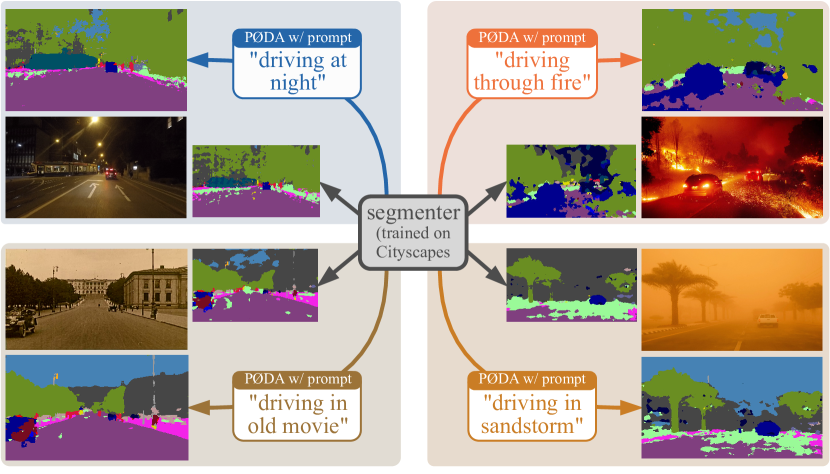
Figure 1: Zero-shot adaptation with prompt. PØDA enables the adaptation of a segmenter model (here, DeepLabv3+ trained on the source dataset Cityscapes) to unseen conditions with only a prompt. Source-only predictions are shown as smaller segmentation masks to the left or right of the test images.

To mitigate this domain-shift problem [2], unsupervised domain adaptation (UDA) [17, 46, 19, 61, 48, 50] has emerged as a promising solution. Training of UDA methods requires labeled data from source domain and unlabeled data from target domain. Though seemingly effortless, for some conditions even collecting unlabeled data is complex. For example, as driving through fire or sandstorm rarely occurs in real life, collecting raw data in such conditions is non-trivial. One may argue on using Internet images for UDA. However, in the industrial context, the practice of using public data is limited or forbidden. Recent works aim to reduce the burden of target data collection campaigns by devising one-shot [34, 56] UDA methods, i.e., using one target image for training. Pushing further this line of research, we frame the challenging new task of prompt-driven zero-shot domain adaptation where given a target domain description in natural language (i.e., a prompt), our method accordingly adapts the segmentation model to this domain of interest. Figure 1 outlines the primary goal of our work with a few qualitative examples. Without seeing any fire or sandstorm images during training, the adapted models succeed in segmenting out critical scene objects, exhibiting fewer errors than the original source-only model.
Our method, illustrated in Fig. 2, is made possible by leveraging the vision-language connections from the seminal CLIP model [40]. Trained on 400M web-crawled image-text pairs, CLIP has revolutionized multi-modal representation learning, bringing outstanding capability to zero-shot image synthesis [25, 16, 38], zero-shot multi-modal fusion [21], zero-shot semantic segmentation [27, 60], open-vocabulary object detection [35], few-shot learning [10], etc. In our work, we exploit the CLIP’s latent space and propose a simple and effective feature stylization mechanism that converts source-domain features into target-domain ones (Fig. 2, left), which can be seen as a specific form of data augmentation. Fine-tuning the segmentation model on these zero-shot synthesized features (Fig. 2, middle) helps mitigating the distribution gap between the two domains thus improving performance on unseen domains (Fig. 2, right). Owing to the standard terminology of “prompt” that designates the input text in CLIP-based image generation, we coin our approach Prompt-driven Zero-shot Domain Adaptation, PØDA in short.

To summarize, our contributions are as follows:

• We introduce the novel task of prompt-driven zero-shot domain adaptation, which aims at adapting a source-trained model on a target domain provided only an arbitrary textual description of the latter.

• Unlike other CLIP-based methods that navigate CLIP latent space using direct image representations, we alter only the features, without relying on the appearance in pixel space. We argue that this is particularly useful for downstream tasks such as semantic segmentation where good features are decisive (and sufficient). We present a simple and effective Prompt-driven Instance Normalization (PIN) layer to augment source features, where affine transformations of low-level features are optimized such that the representation in CLIP latent space matches the one of target-domain prompt.

• We show the versatility of our method by adapting source-trained semantic segmentation models to different conditions: (i) from clear weather/daytime to adverse conditions (snow, rain, night), (ii) from synthetic to real, (iii) from real to synthetic. Interestingly, PØDA outperforms state-of-the-art one-shot unsupervised domain adaptation without using any target image.

• We show that PØDA can also be applied to object detection and image classfication.

2 Related works

Unsupervised Domain Adaptation.  The UDA literature is vast and encompasses different yet connected approaches: adversarial learning [17, 48], self-training [62, 30], entropy minimization [50, 37], generative-based adaptation [19], etc. The domain gap is commonly reduced at the level of the input [19, 57], of the features [17, 46, 54, 33] or of the output [48, 50, 37].

Recently, the more challenging setting of One-Shot Unsupervised Domain Adaptation (OSUDA) has been proposed. To the best of our knowledge, two works on OSUDA for semantic segmentation exist [34, 56]. Luo et al. [34] show that traditional UDA methods fail when only a single unlabeled target image is available. To mitigate the risk of over-fitting on the style of the single available image, the authors propose a style mining algorithm, based on both a stylized image generator and a task-specific module. Wu et al. [56] introduce an approach based on style mixing and patch-wise prototypical matching (SM-PPM). During training, channel-wise mean and standard deviation of a randomly sampled source image’s features are linearly mixed with the target ones. Patch-wise prototypical matching helps overcome negative adaptation [28].

In the more challenging zero-shot setting (where no target image is available), Lengyel et al. [26] tackle day-to-night domain adaptation using physics priors. They introduce a color invariant convolution layer (CIConv) that is added to make the network invariant to different lighting conditions. We note that this zero-shot adaption is orthogonal to ours and restricted to a specific type of domain gap.

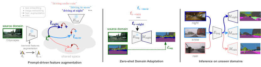
Figure 2: Overview of PØDA, a Prompt-driven Zero-shot Domain Adaptation. (Left) Using only a single textual description (“…”) of an unseen target domain, we leverage a frozen ResNet encoder with CLIP weights to learn $\text{source}{\shortrightarrow}\text{target}$ low-level feature stylizations. Applied to a source image low-level feature map ${\mathbf{f}}_{\text{s}}$ with latent embedding $\color[rgb]{0.0,0.4375,0.0}\bar{\mathbf{f}}_{\text{s}}$, these stylizations provide augmented features $\mathbf{f}_{\text{s}\shortrightarrow\text{t}}$ which embeddings (here, $\color[rgb]{0.0,0.0,0.8}\bar{\mathbf{f}}_{\text{night}}$, $\color[rgb]{0.2,0.6,1.0}\bar{\mathbf{f}}_{\text{snow}}$, $\color[rgb]{1.0,0.48,0.48}\bar{\mathbf{f}}_{\text{rain}}$) are closer to their respective target prompt embeddings (+). (Middle) Zero-shot domain adaptation is achieved by fine-tuning a segmenter model ($M$) on the feature-augmented source domain with the learned transformations. (Right) This enables inference on unseen domains.

Text-driven image synthesis.  Recently, contrastive image-language pretraining has shown unprecedented success for multimodal learning in several downstream tasks such as zero-shot classification [40], multi-modal retrieval [22] and visual question answering [29]. This encouraged the community to modify images using text descriptions, a task that was previously challenging due to the gap between vision and language representations. For example, StyleCLIP [38] uses prompts to optimize StyleGAN [23] latent vectors and guide the generation process. However, the generation is limited to the training distribution of StyleGAN. To overcome this issue, StyleGAN-NADA [16] utilizes CLIP embeddings of text-prompts to perform domain adaptation of the generator, which is in this case trainable. Similarly, for text-guided semantic image editing, FlexIT [12] optimizes the latent code in VQGAN autoencoder’s[14] space.

For text-guided style transfer, CLIPstyler [25] does not rely on a generative process. This setting is more realistic for not being restricted to a specific distribution, and challenging at the same time for the use of the encapsulated information in CLIP latent space. Indeed, there is no one-to-one mapping between image and text representations and regularization is needed to extract the useful information from a text embedding. Thus, in the same work [25], a U-net autoencoder that preserves the content is optimized while the output image embedding in CLIP latent space is varying during the optimization process.

We note that a common point in prior works is the mapping from pixel-space to CLIP latent space during the optimization process. In contrast with this, we directly manipulate deep features of the pre-trained CLIP visual encoder.

3 Prompt-driven Zero-shot Adaptation

Our framework, illustrated in Fig. 2, builds upon CLIP [40], a vision-language model pre-trained on 400M image-text pairs crawled from the Internet. CLIP trains jointly an image encoder $E_{\text{img}}$ and a text encoder $E_{\text{txt}}$ over many epochs and learns an expressive representation space that effectively bridges the two modalities. In this work, we leverage this property to “steer” features from any source image towards a target domain in the CLIP latent space, with guidance from an arbitrary prompt describing the target domain, e.g., “driving at night” or “navigating the roads in darkness” for the night domain. Our goal is to modify the style of source image features, bringing them closer to imaginary counterparts in the targeted domain (Fig. 2, left), while preserving their semantic content. The learned augmentations can then be applied on source images to generate features, in a zero-shot fashion, that correspond to the unseen target domain and can be further used to fine-tune the model towards handling target domain (Fig. 2, middle). This ultimately allows inference on unseen domains only described by a simple prompt at train time (Fig. 2, right).

Our approach faces several challenges: (i) How to generate informative features for the target domain without having access to any image from it; (ii) How to preserve pixel-wise semantics while augmenting features; (iii) Based on such features, how to adapt the source model to the unseen target domain. We address these questions in the following.

Problem formulation.  Our main task is semantic segmentation, that is, pixel-wise classification of input image into semantic segments. We start from a $K$-class segmentation model $M$, pre-trained on a source domain dataset ${\mathcal{D}}_{\text{s}}=\{({\mathbf{x}}_{\text{s}},{\mathbf{y}}_{\text{s}})\mid{\mathbf{x}}_{\text{s}}\in\mathbb{R}^{H\times W\times 3},{\mathbf{y}}_{\text{s}}\in\{0,1\}^{H\times W\times K}\}$. By using a single predefined prompt $\mathsf{TrgPrompt}$ describing the targeted domain, we adapt the model $M$ such that its performance on the unseen test target dataset ${\mathcal{D}}_{\text{t}}=\{{\mathbf{x}}_{\text{t}}\mid{\mathbf{x}}_{\text{t}}\in\mathbb{R}^{H\times W\times 3}\}$ is improved. The segmenter $M$ is a DeepLabv3+ model [6] with CLIP image encoder $E_{\text{img}}$ (e.g., ResNet-50) as the frozen feature extractor backbone $M_{\text{feat}}$ and a randomly initialized pixel classification head $M_{\text{cls}}$: $M=(M_{\text{feat}},M_{\text{cls}})$. We train $M$ in a supervised manner for the semantic segmentation task on the source domain. In order to preserve the compatibility of the encoder features with the CLIP latent space we keep $M_{\text{feat}}$ frozen and train only the pixel classifier $M_{\text{cls}}$. Interestingly, we empirically show in Tab. 1 that keeping the feature extractor $M_{\text{feat}}$ frozen also prevents overfitting to the source in favor of generalization. From the extractor we remove the attention pooling head of $E_{\text{img}}$ to keep the spatial information for the pixel classifier. We denote $\mathbf{f}$ the intermediate features extracted by $M_{\text{feat}}$ and $\bar{\mathbf{f}}$ their corresponding CLIP embedding computed with the attention pooling layer of $E_{\text{img}}$. In Fig. 3 we illustrate the difference between $\mathbf{f}$ and $\bar{\mathbf{f}}$.

$M_{\text{feat}}$ 2744	CS	Night	Snow	Rain	GTA5
Yes	66.82	18.31	39.28	38.20	39.59
No	69.17	14.40	22.27	26.33	32.91

Table 1: Segmentation with source-only trained models. Performance (mIoU %) on “night”, “snow” and “rain” parts of ACDC [45] validation set and on a subset of $1000$ GTA5 images for models trained on Cityscapes (CS). ‘$M_{\text{feat}}$2744’: frozen backbone.

Overview of the proposed method.  Our solution is to mine styles using source-domain low level features set ${\mathcal{F}}_{\text{s}}{=}\{{\mathbf{f}}_{\text{s}}{\mid}{\mathbf{f}}_{\text{s}}{=}\texttt{feat-ext}(M_{\text{feat}},{\mathbf{x}}_{\text{s}})\}$ and $\mathsf{TrgEmb}$, where $\mathsf{TrgEmb}{=}E_{\text{txt}}(\mathsf{TrgPrompt})$ is the CLIP text embedding of the target domain prompt. For generality, $\texttt{feat-ext}(\cdot)$ can pull features from any desired layer but we later show that using the lowest features works best.

1

Input : Set ${\mathcal{F}}_{\text{s}}$ of source image features

Target domain description embedding $\mathsf{TrgEmb}$

Param : Number $N$ of optimization steps

Learning rate $lr$ and momentum $m$

 of gradient descend (GD)

Output : Set ${\mathcal{S}}_{\text{s}\shortrightarrow\text{t}}$ of target styles

2

3${\mathcal{S}}_{\text{s}\shortrightarrow\text{t}}\leftarrow\emptyset$

4 foreach ${\mathbf{f}}_{\text{s}}\in{\mathcal{F}}_{\text{s}}$ do

5      $\bm{\mu}^{0}\leftarrow\textnormal{{mean}}({\mathbf{f}}_{\text{s}})$

6       $\bm{\sigma}^{0}\leftarrow\textnormal{{std}}({\mathbf{f}}_{\text{s}})$

       // Optimization

7       for $\text{i}=1,2,\cdots,N$ do

8            $\mathbf{f}_{\text{s}\shortrightarrow\text{t}}^{i}\leftarrow\textnormal{{PIN}}({\mathbf{f}}_{\text{s}},\bm{\mu}^{i-1},\bm{\sigma}^{i-1})$

9             $\bar{\mathbf{f}}_{\text{s}\shortrightarrow\text{t}}^{i}\leftarrow\textnormal{{get-embedding}}(\mathbf{f}_{\text{s}\shortrightarrow\text{t}}^{i})$

10             $\bm{\mu}^{i}\leftarrow\texttt{GD}^{lr}_{m}(\bm{\mu}^{i-1},\nabla_{\bm{\mu}}\mathcal{L}_{\bm{\mu},\bm{\sigma}}(\bar{\mathbf{f}}_{\text{s}\shortrightarrow\text{t}}^{i},\mathsf{TrgEmb}))$

11             $\bm{\sigma}^{i}\leftarrow\texttt{GD}^{lr}_{m}(\bm{\sigma}^{i-1},\nabla_{\bm{\sigma}}\mathcal{L}_{\bm{\mu},\bm{\sigma}}(\bar{\mathbf{f}}_{\text{s}\shortrightarrow\text{t}}^{i},\mathsf{TrgEmb}))$

12       end for

13      $(\bm{\mu}_{t},\bm{\sigma}_{t})\leftarrow(\bm{\mu}^{N},\bm{\sigma}^{N})$

14       ${\mathcal{S}}_{\text{s}\shortrightarrow\text{t}}\leftarrow{\mathcal{S}}_{\text{s}\shortrightarrow\text{t}}\cup\{(\bm{\mu}_{t},\bm{\sigma}_{t})\}$

15 end foreach

Algorithm 1 Style Mining (see Fig. 3)

The $\texttt{augment}(\cdot)$ operation, depicted in Fig. 3, augments the style-specific components of ${\mathbf{f}}_{\text{s}}$ with guidance from the target domain prompt, synthesizing ${\mathbf{f}}_{\text{s}\shortrightarrow\text{t}}$ with style information from the target domain. We emphasize that the features ${\mathbf{f}}_{\text{s}}$ and ${\mathbf{f}}_{\text{s}\shortrightarrow\text{t}}$ have the same size $h\times w\times c$ and identical semantic content, though they encapsulate different visual styles. For adaptation, the source features ${\mathbf{f}}_{\text{s}}$ are augmented with the mined styles then used to fine-tune the classifier $M_{\text{cls}}$, resulting in the final adapted model. The overall pseudo-code is provided in Supplementary Material.

3.1 Zero-shot Feature Augmentation

We take inspiration from Adaptive Instance Normalization (AdaIN) [20], an elegant formulation for transferring style-specific components across deep features. In AdaIN, the styles are represented by the channel-wise mean $\bm{\mu}\in\mathbb{R}^{c}$ and standard deviation $\bm{\sigma}\in\mathbb{R}^{c}$ of features, with $c$ the number of channels. Stylizing a source feature ${\mathbf{f}}_{\text{s}}$ with an arbitrary target style $(\mu({\mathbf{f}}_{\text{t}}),\sigma({\mathbf{f}}_{\text{t}}))$ reads:

$$\small\texttt{AdaIN}({\mathbf{f}}_{\text{s}},{\mathbf{f}}_{\text{t}})=\sigma({\mathbf{f}}_{\text{t}})\left(\frac{{\mathbf{f}}_{\text{s}}-\mu({\mathbf{f}}_{\text{s}})}{\sigma({\mathbf{f}}_{\text{s}})}\right)+\mu({\mathbf{f}}_{\text{t}}),$$ (1)

with $\mu(\cdot)$ and $\sigma(\cdot)$ as the two functions returning channel-wise mean and standard deviation of input feature; multiplications and additions are element-wise.

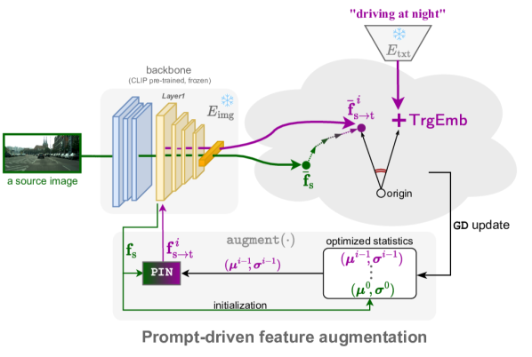
Figure 3: Target style mining from a source image. We illustrate here the optimization loops of Algorithm 1. The source image is forwarded through the CLIP image encoder $E_{\text{img}}$ to extract low-level features $\color[rgb]{0.0,0.4375,0.0}{\mathbf{f}}_{\text{s}}$ and subsequent CLIP embedding $\color[rgb]{0.0,0.4375,0.0}{\bar{\mathbf{f}}}_{\text{s}}$. At each optimization step $i$, $\texttt{augment}(\cdot)$ takes the style of the previous iteration, $\color[rgb]{0.5977,0.0,0.5977}(\bm{\mu}^{i-1}\!\!,\bm{\sigma}^{i-1})$ and injects it within $\color[rgb]{0.0,0.4375,0.0}{\mathbf{f}}_{\text{s}}$ via the PIN layer, to synthesize $\color[rgb]{0.5977,0.0,0.5977}\textbf{f}^{i}_{\text{s}\shortrightarrow\text{t}}$ and the corresponding embedding $\color[rgb]{0.5977,0.0,0.5977}\bar{\textbf{f}}^{i}_{\text{s}\shortrightarrow\text{t}}$. The loss $\color[rgb]{0,0,0}\mathcal{L}_{\bm{\mu},\bm{\sigma}}$ is the cosine distance between $\color[rgb]{0.5977,0.0,0.5977}\bar{\textbf{f}}^{i}_{\text{s}\shortrightarrow\text{t}}$ and the target prompt embedding $\mathsf{TrgEmb}$. Its optimization via gradient descent updates style to ${\color[rgb]{0.5977,0.0,0.5977}(\bm{\mu}^{i}\!,\bm{\sigma}^{i})}$.

We design our augmentation strategy around AdaIN as it can effectively manipulate the style information with a small set of parameters. In the following, we present our augmentation strategy which mines target styles.

As we do not have access to any target (i.e. style) image, $\mu({\mathbf{f}}_{\text{t}})$ and $\sigma({\mathbf{f}}_{\text{t}})$ are unknown. Thus, we propose Prompt-driven Instance Normalization (PIN):

$$\small\texttt{PIN}({\mathbf{f}}_{\text{s}},\bm{\mu},\bm{\sigma})=\bm{\sigma}\left(\frac{{\mathbf{f}}_{\text{s}}-\mu({\mathbf{f}}_{\text{s}})}{\sigma({\mathbf{f}}_{\text{s}})}\right)+\bm{\mu},$$ (2)

where ${\bm{\mu}}$ and ${\bm{\sigma}}$ are optimizable variables driven by a prompt.

We aim to augment source image features ${\mathcal{F}}_{\text{s}}$ such that they capture the style of the target domain. Here, the prompt describing a target domain could be fairly generic. For instance, one can use prompts like “driving at night” or “driving under rain” to bring source features closer to the nighttime or rainy domains. The prompt is processed by the CLIP text encoder $E_{\text{txt}}$ into the $\mathsf{TrgEmb}$ embedding.

We describe in Algorithm 1 the first step of our zero-shot feature augmentation procedure: mining the set ${\mathcal{S}}_{\text{s}\shortrightarrow\text{t}}$ of styles in targeted domain. For each source feature map ${\mathbf{f}}_{\text{s}}\in{\mathcal{F}}_{\text{s}}$, we want to mine style statistics corresponding to an imaginary target feature map ${\mathbf{f}}_{\text{t}}$. To this end, we formulate style mining as an optimization problem over the original source feature ${\mathbf{f}}_{\text{s}}$, i.e. optimizing $(\bm{\mu},\bm{\sigma})$ in Eq. 2. The optimization objective is defined as the cosine distance in the CLIP latent space between the CLIP embedding $\bar{\mathbf{f}}_{\text{s}\shortrightarrow\text{t}}$ of the stylized feature ${\mathbf{f}}_{\text{s}\shortrightarrow\text{t}}=\texttt{PIN}({\mathbf{f}}_{\text{s}},\bm{\mu},\bm{\sigma})$ and the description embedding $\mathsf{TrgEmb}$ of target domain:

$$\small\mathcal{L}_{\bm{\mu},\bm{\sigma}}(\bar{\mathbf{f}}_{\text{s}\shortrightarrow\text{t}},\mathsf{TrgEmb})=1-\frac{\bar{\mathbf{f}}_{\text{s}\shortrightarrow\text{t}}\cdot\mathsf{TrgEmb}}{\|\bar{\mathbf{f}}_{\text{s}\shortrightarrow\text{t}}\|\,\|\mathsf{TrgEmb}\|}\,.$$ (3)

This CLIP-space cosine distance, already used in prior text-driven image editing works [38], aims to steer the stylized features in the direction of the target text embedding. One step of the optimization is illustrated in Fig. 3. In practice, we run several such steps leading to the mined target style denoted $(\bm{\mu}_{t},\bm{\sigma}_{t})$.

As there might be a variety of styles in a target domain, our mining populates the ${\mathcal{S}}_{\text{s}\shortrightarrow\text{t}}$ set with as many variations of target style as there are source images, hence $|{\mathcal{S}}_{\text{s}\shortrightarrow\text{t}}|=|{\mathcal{D}}_{\text{s}}|$.

Intuitively, our simple augmentation strategy can be seen as a cost-efficient way to cover the distribution of the target domain by starting from different anchor points in the CLIP latent space coming from the source images and steering them in the direction of the target text embedding. This mitigates the diversity problem discussed in one-shot feature augmentation in [34, 56].

3.2 Fine-tuning for Adaptation

For adaptation, at each training iteration we stylize the source features using a mined target style $({\bm{\mu}}_{t},\bm{\sigma}_{t})$ randomly selected from ${\mathcal{S}}_{\text{s}\shortrightarrow\text{t}}$. The augmented features are computed as $\mathbf{f}_{\text{s}\shortrightarrow\text{t}}=\texttt{PIN}({\mathbf{f}}_{\text{s}},\bm{\mu}_{t},\bm{\sigma}_{t})$ and are used for fine-tuning the classifier $M_{\text{cls}}$ of the segmenter $M$ (Fig. 2, middle). As we only adjust the feature style which keeps the semantic-content unchanged [20], we can still use the labels ${{\mathbf{y}}_{\text{s}}}$ to train the classifier with a standard segmentation loss. To this end, we simply forward augmented features through remaining layers in $M_{\text{feat}}$ followed by $M_{\text{cls}}$. In the backward pass, only weights of $M_{\text{cls}}$ are updated by the loss gradients. We denote the fine-tuned model as $M^{\prime}=(M_{\text{feat}},M^{\prime}_{\text{cls}})$ and evaluate it on images with conditions and styles which were never seen during any of the training stages.

4 PØDA for semantic segmentation

4.1 Implementation details

We use the DeepLabv3+ architecture [6] with the backbone $M_{\text{feat}}$ initialized from the image encoder $E_{\text{img}}$ of the pre-trained CLIP-ResNet-50 model.

Source-only training.  The network is trained for $200$k iterations on random $768\times 768$ crops with batch size $2$. We use a polynomial learning rate schedule with initial $lr{=}10^{-1}$ for the classifier and $lr{=}10^{-4}$ for backbone when not frozen (see Tab. 1). We optimize with Stochastic Gradient Descent [4], momentum $0.9$ and weight decay $10^{-4}$. We apply standard color jittering and horizontal flip to crops.

Zero-shot feature augmentation.  For the feature augmentation step, we use the source feature maps after the first layer (Layer1): ${\mathbf{f}}_{\text{s}}\in\mathbb{R}^{192\times 192\times 256}$. The style parameters $\bm{\mu}$ and $\bm{\sigma}$ are $256$D real vectors. The CLIP embeddings are $1024$D vectors. We adopt the Imagenet templates from [40] to encode the target descriptions in $\mathsf{TrgPrompt}$.

Classifier fine-tuning.  Starting from the source-only pre-trained model, we fine-tune the classifier $M_{\text{cls}}$ on batches of $8$ augmented features ${\mathbf{f}}_{\text{s}\shortrightarrow\text{t}}$ for $2,000$ iterations. Polynomial schedule is used with the initial $lr=10^{-2}$. We always use the last checkpoint for evaluation.

Datasets.  As source, we use Cityscapes [11], composed of $2,975$ training and $500$ validation images featuring $19$ semantic classes. Though we adapt towards a prompt not a dataset, we need adhoc datasets to test on. We report main results using ACDC [45] because it has urban images captured in adverse conditions. We also study the applicability of PØDA to the two settings of real$\shortrightarrow$synthetic (Cityscapes as source, and evaluating on GTA5 [43]) and synthetic$\shortrightarrow$real (GTA5 as source, and evaluating on Cityscapes). We evaluate on the validation set when provided, and for GTA5 evaluation we use a random subset of $1,000$ images.

Evaluation protocol.  Mean Intersection over Union (mIoU%) is used to measure adaptation performance. We test all models on target images at their original resolutions. For baselines and PØDA, we always report the mean and standard deviation over five models trained with different random seeds.

4.2 Main results

We consider the following adaptation scenarios: day$\shortrightarrow$night, clear$\shortrightarrow$snow, clear$\shortrightarrow$rain,  real$\shortrightarrow$synthetic and synthetic$\shortrightarrow$real. We report zero-shot adaption results of PØDA in the addressed set-ups, comparing against two state-of-the-art baselines: CLIPstyler [25] for zero-shot style transfer and SM-PPM [56] for one-shot UDA. Both PØDA and CLIPstyler models see no target images during training. In this study, we arbitrarily choose a simple prompt to describe each domain. We show later in Sec. 4.3 more results using other relevant prompts with similar meanings – showcasing that our adaptation gain is little sensitive to prompt selection. For SM-PPM, one random target image from the training set is used.

Comparison to CLIPstyler [25].  CLIPstyler is a style transfer method that also makes use of the pre-trained CLIP model but for zero-shot stylizing of source images. We consider CLIPstyler as the most comparable zero-shot baseline for PØDA as both are built upon CLIP, though with different mechanisms and different objectives. Designed for style transfer, CLIPstyler produces images that exhibit characteristic styles of the input text prompt. However the stylized images can have multiple artifacts which hinder their usability in the downstream segmentation task. This is visible in Fig. 4 which shows stylized examples from CLIPstyler with PØDA target prompts. Zooming in, we note that stylization of snow or game added snowy roads or Atari game on the buildings, respectively.

Starting from source-only model, we fine-tune the classifier on stylized images, as similarly done in PØDA with the augmented features. Table 2 compares PØDA against the source-only model and CLIPstyler. PØDA consistently outperforms the two baselines. CLIPstyler brings some improvements over source-only in Cityscapes$\shortrightarrow$Night and Cityscapes$\shortrightarrow$Snow. In other scenarios, e.g., rain, CLIPstyler even performs worse than source-only.

Source	Target eval.	Method	mIoU[%]
CS	$\mathsf{TrgPrompt}$ = “driving at night”
	ACDC Night	source-only	18.31 $\pm$0.00
		CLIPstyler	21.38 $\pm$0.36
		PØDA	25.03 $\pm$0.48
	$\mathsf{TrgPrompt}$ = “driving in snow”
	ACDC Snow	source-only	39.28 $\pm$0.00
		CLIPstyler	41.09 $\pm$0.17
		PØDA	43.90 $\pm$0.53
	$\mathsf{TrgPrompt}$ = “driving under rain”
	ACDC Rain	source-only	38.20 $\pm$0.00
		CLIPstyler	37.17 $\pm$0.10
		PØDA	42.31 $\pm$0.55
	$\mathsf{TrgPrompt}$ = “driving in a game”
	GTA5	source-only	39.59 $\pm$0.00
		CLIPstyler	38.73 $\pm$0.16
		PØDA	41.07 $\pm$0.48
GTA5	$\mathsf{TrgPrompt}$ = “driving”
	CS	source-only	36.38 $\pm$0.00
		CLIPstyler	31.50 $\pm$0.21
		PØDA	40.08 $\pm$0.52

Table 2: Zero-shot domain adaptation in semantic segmentation. Performance (mIoU%) of PØDA compared against CLIPstyler [25] and source-only baseline. Results are grouped by source domain and $\mathsf{TrgPrompt}$. CS stands for Cityscapes [11]. The $\mathsf{TrgPrompt}$s are simply chosen, not engineered.

	Cityscapes	night	snow	rain	game

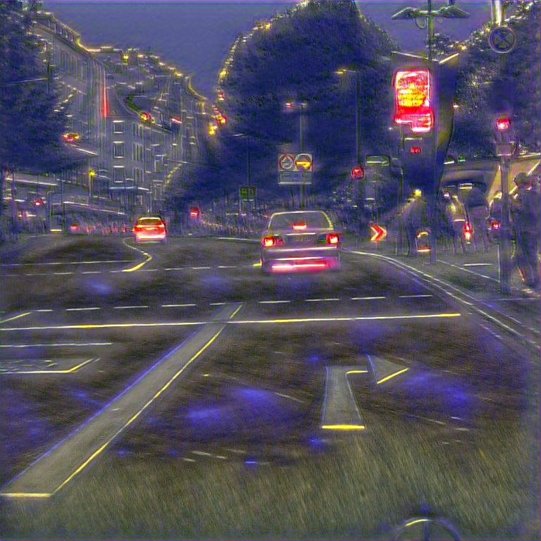
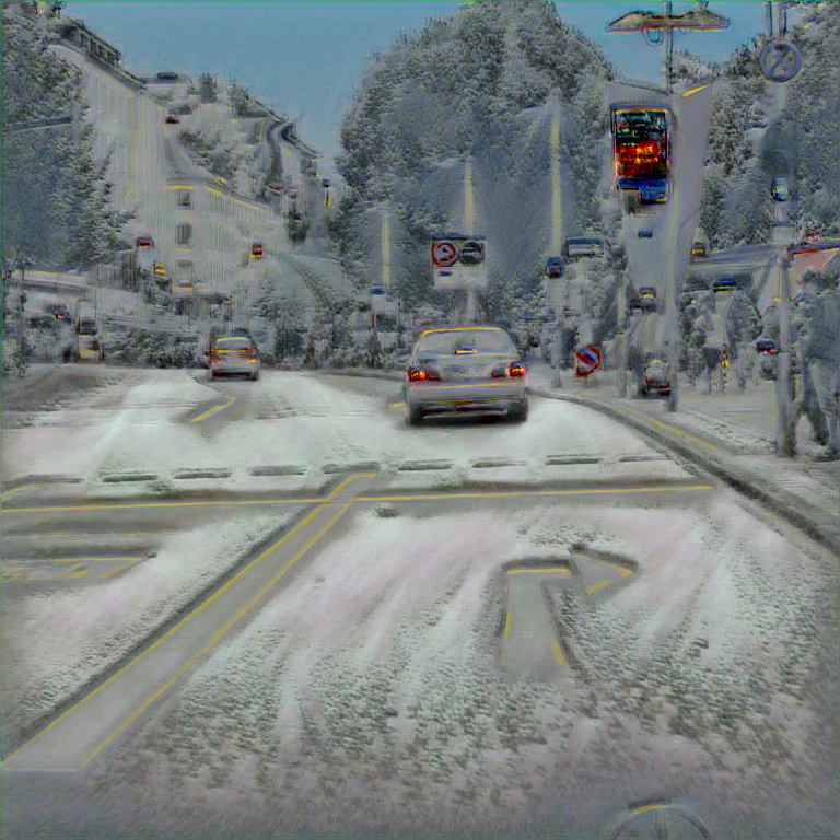
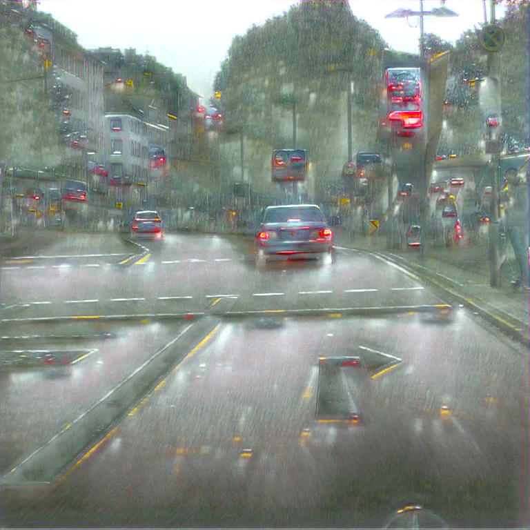
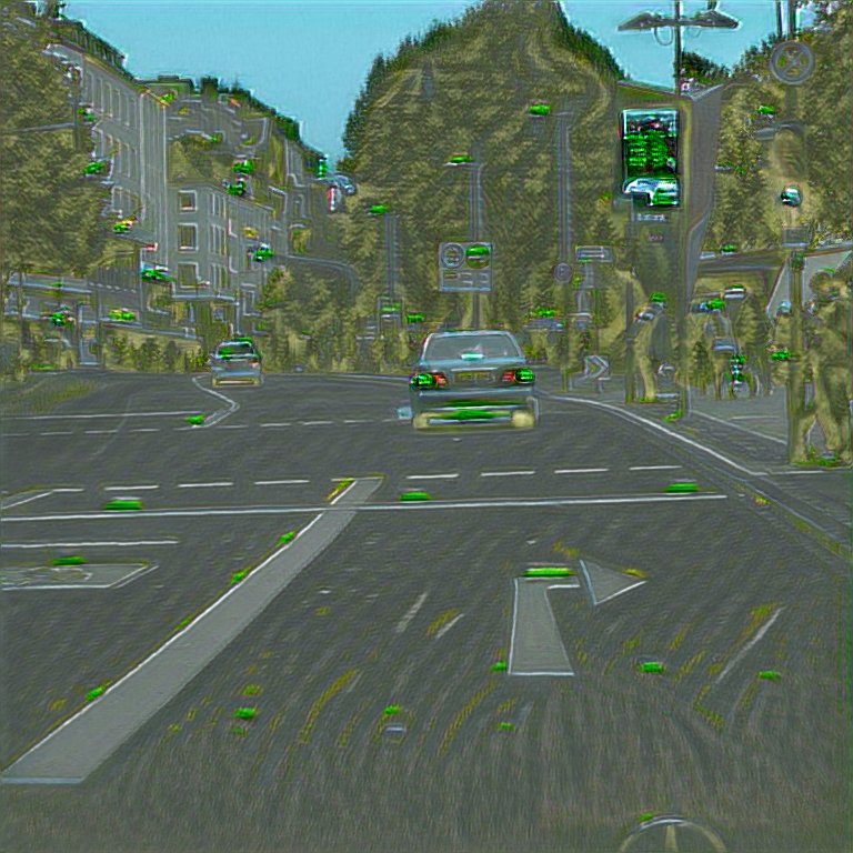
Figure 4: CLIPstyler [25] stylization. A sample Cityscapes image stylized using adhoc target prompts. Translated images exhibit visible artifacts, potentially harming adaptation, e.g. rain in Tab. 2

	input	ground truth	source-only	PØDA
CS$\shortrightarrow$Night
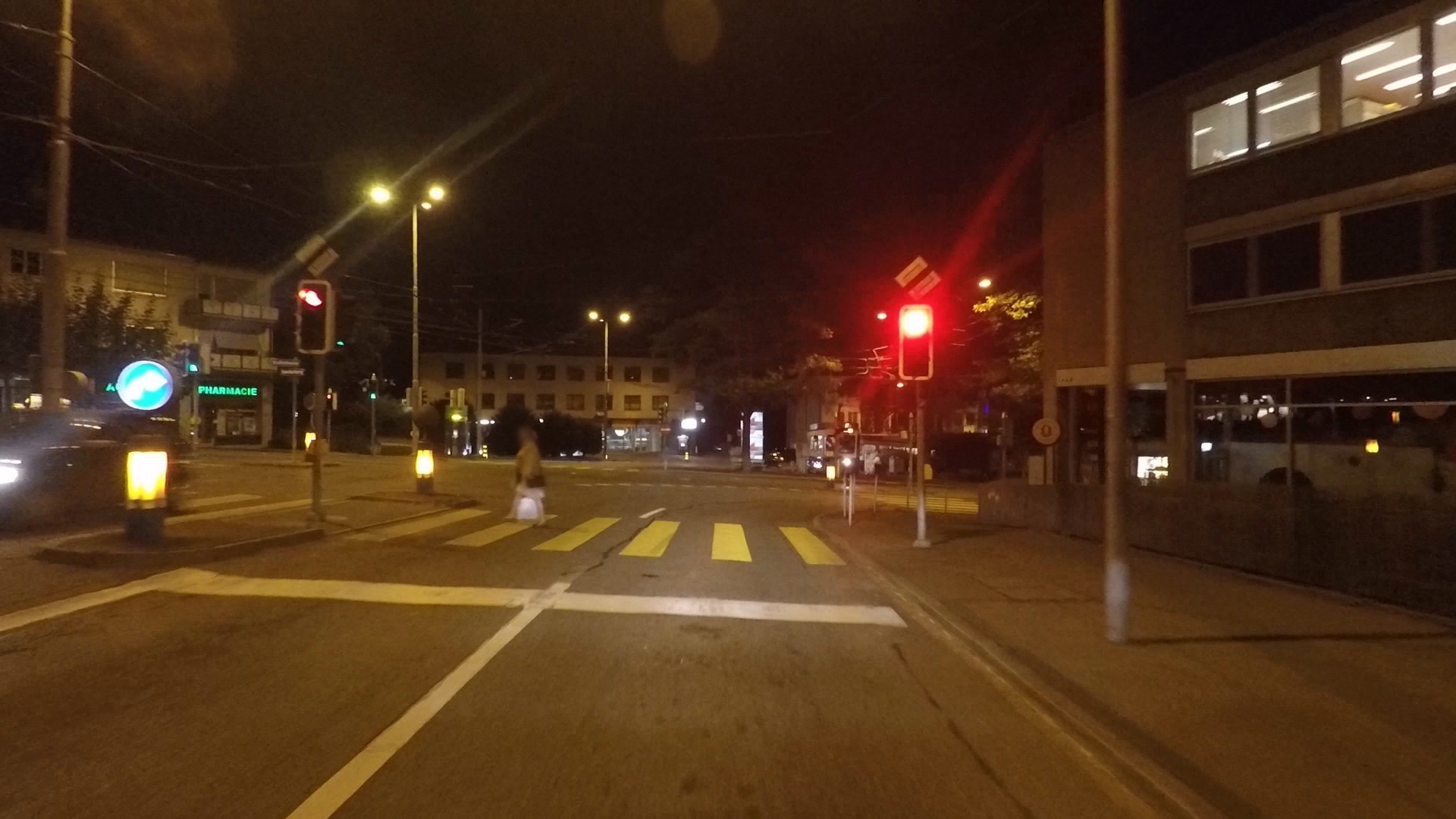
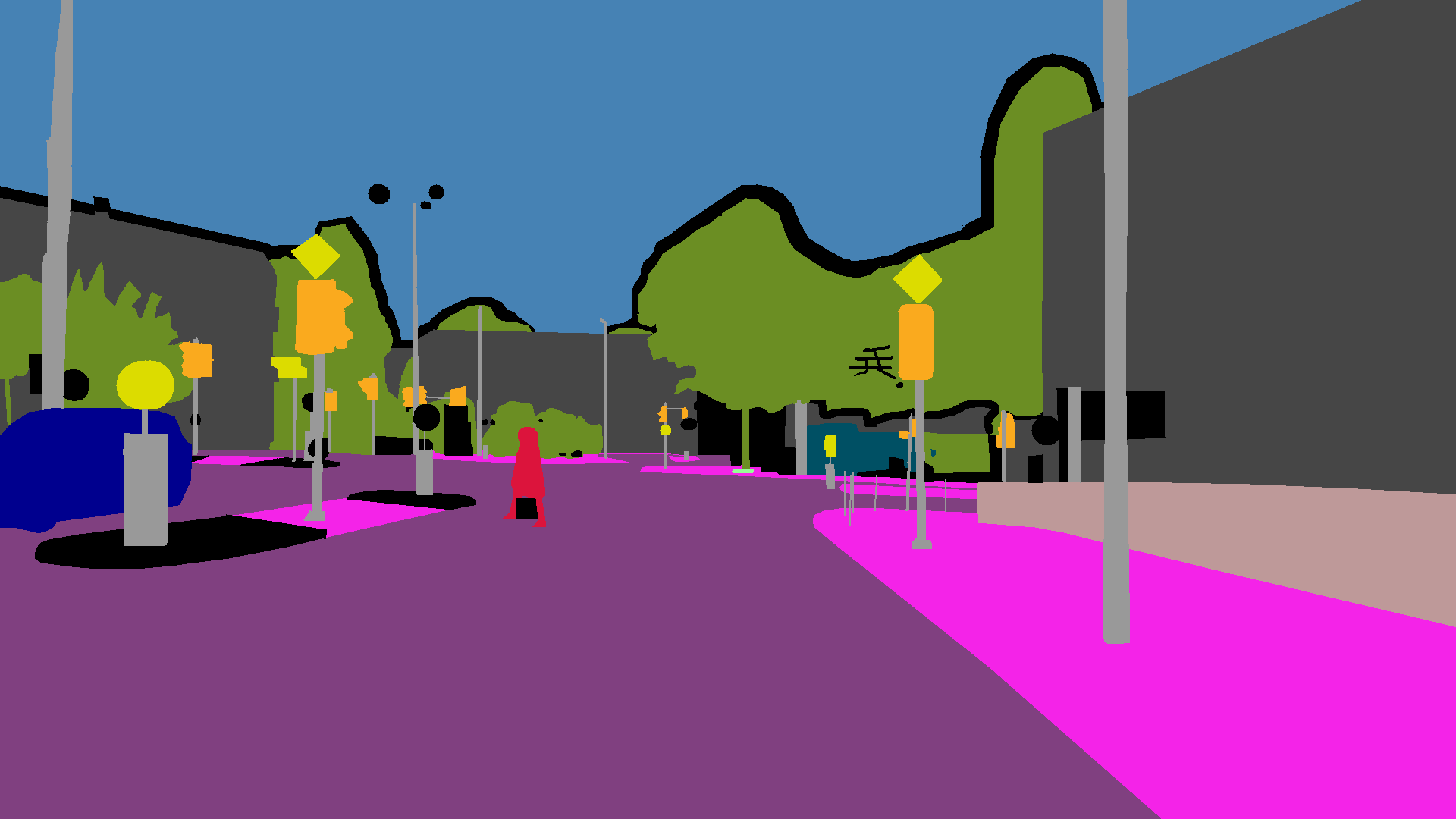
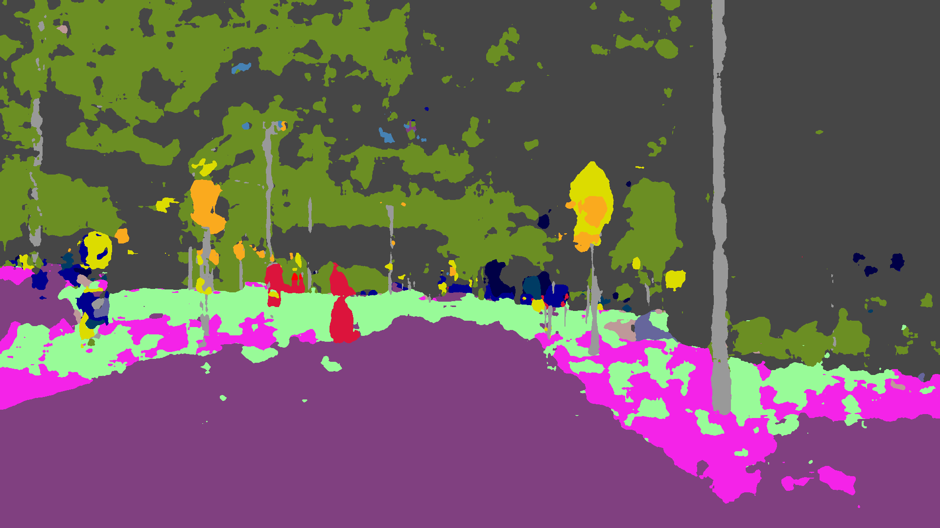
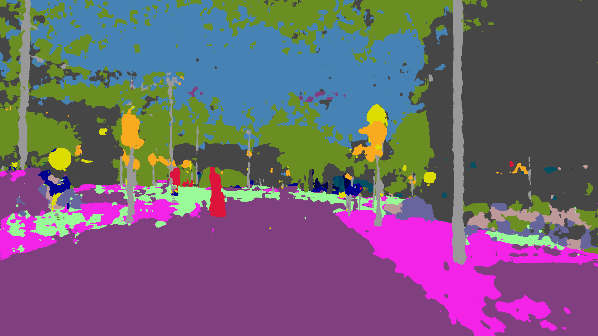
CS$\shortrightarrow$Rain
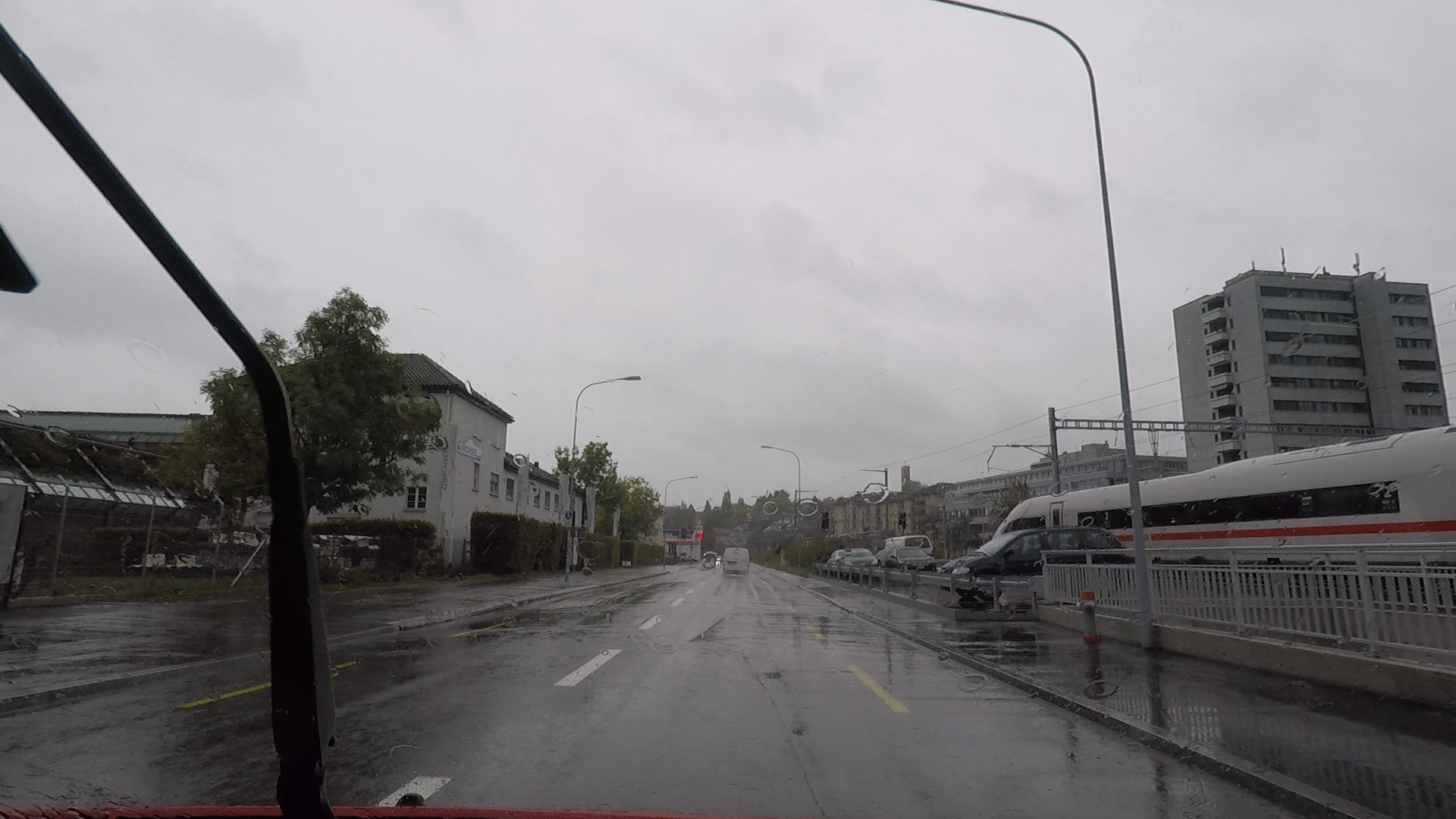
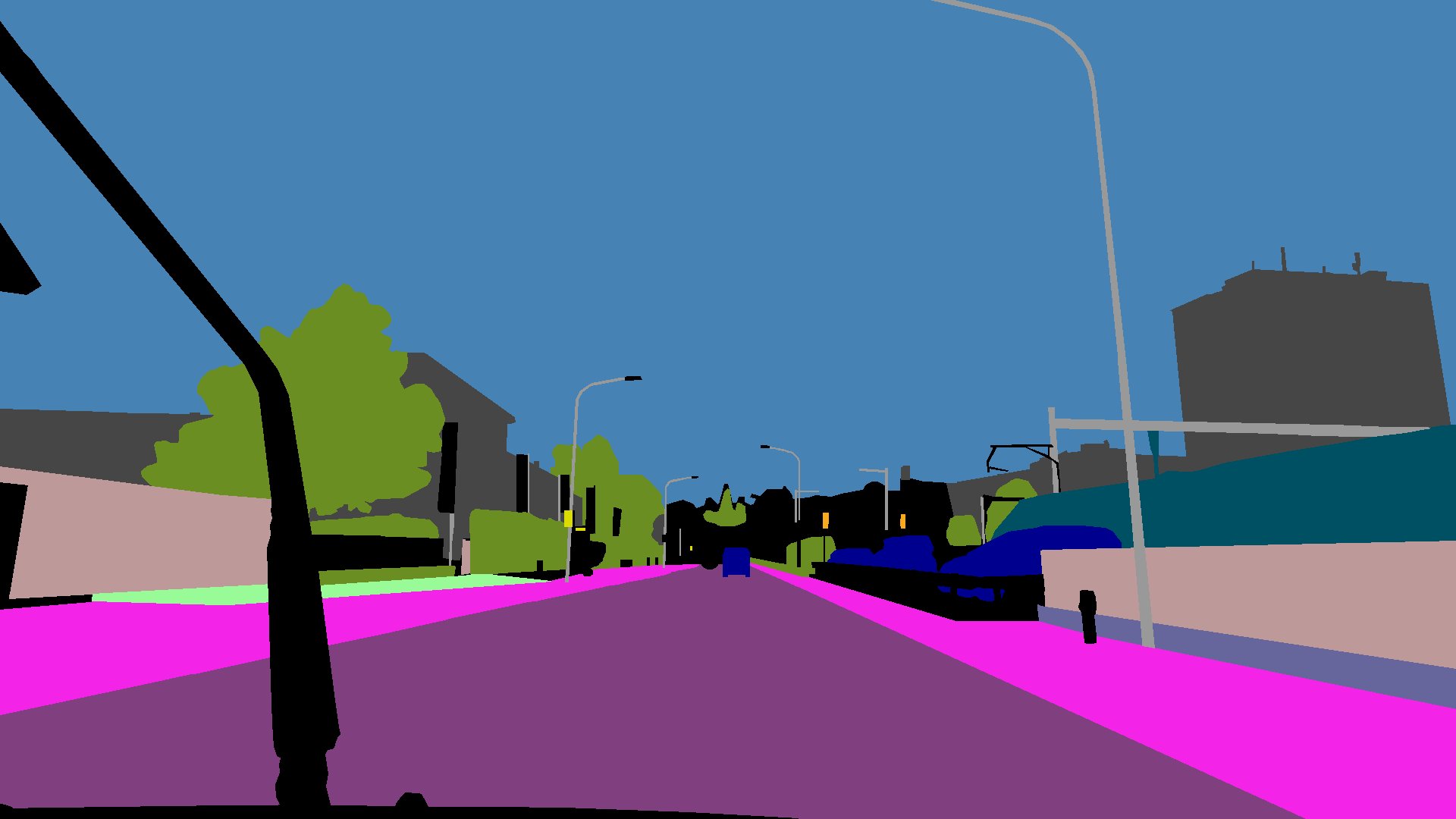
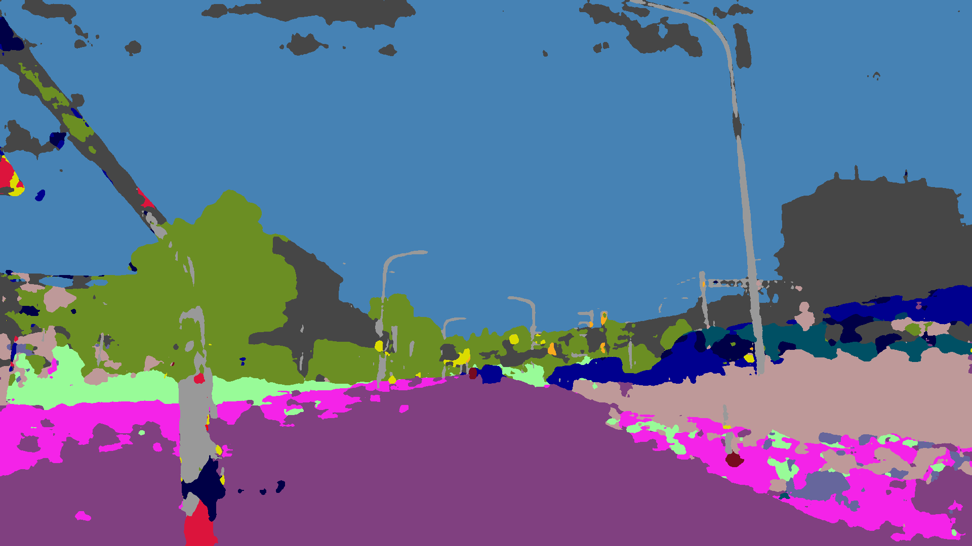
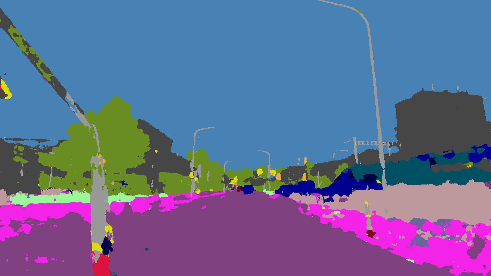
GTA5$\shortrightarrow$Real

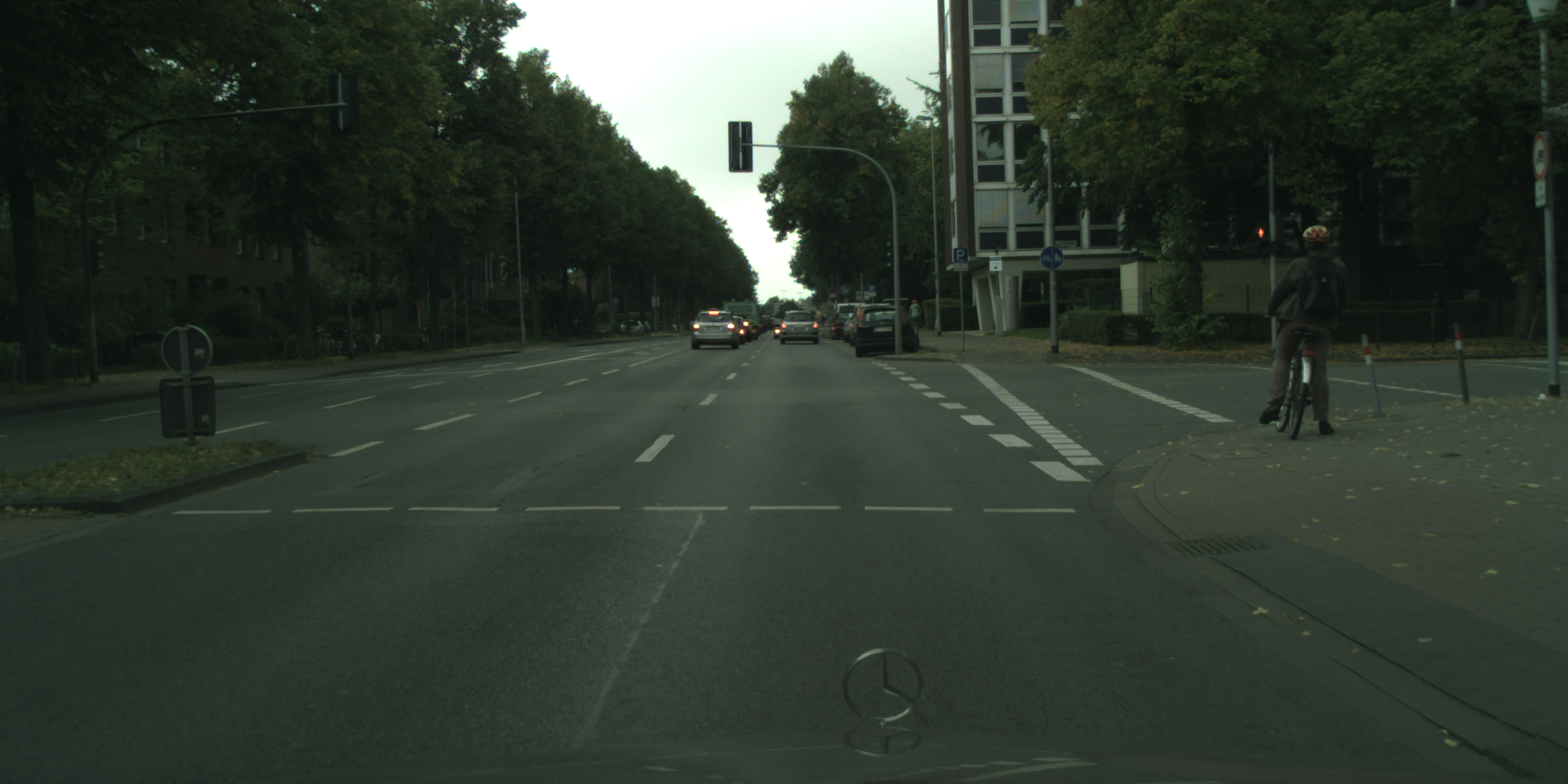
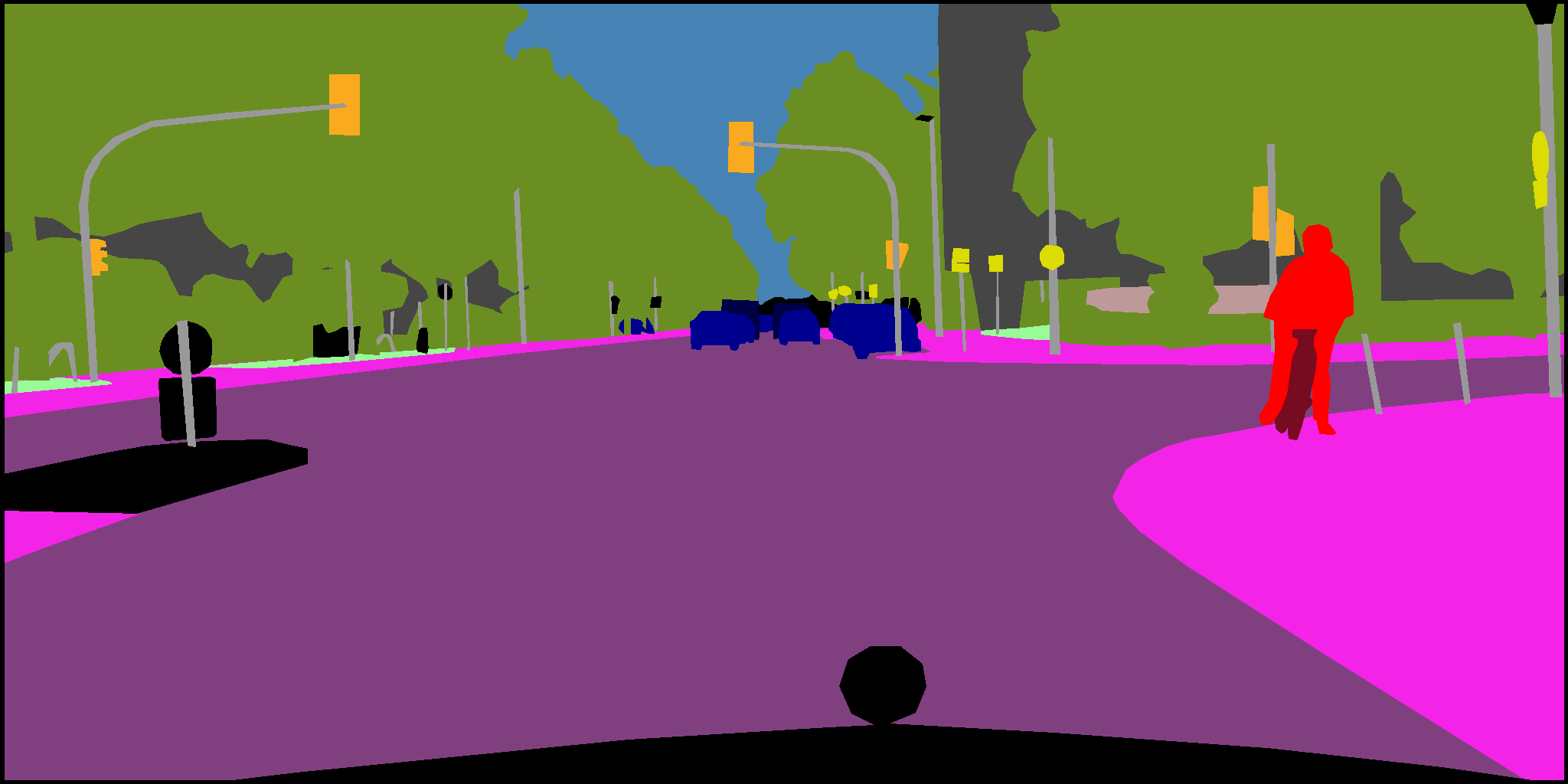
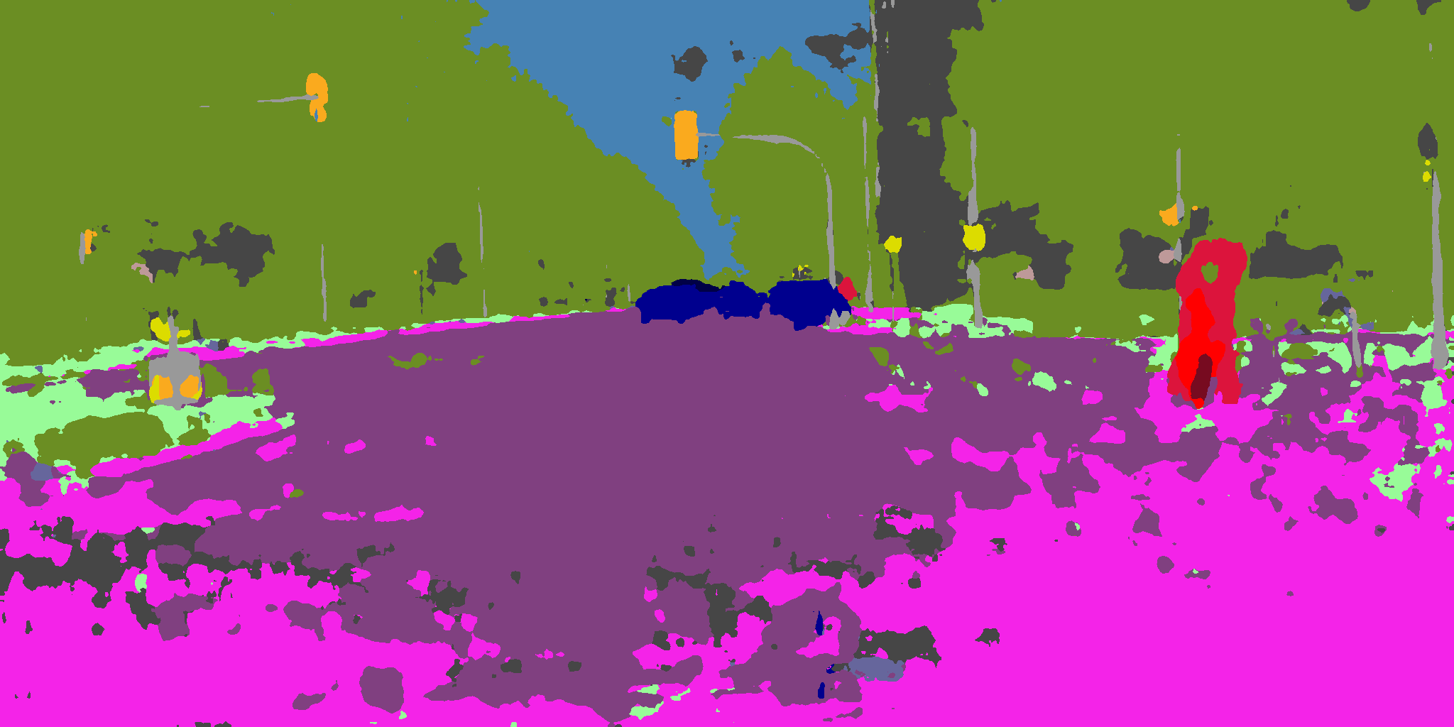
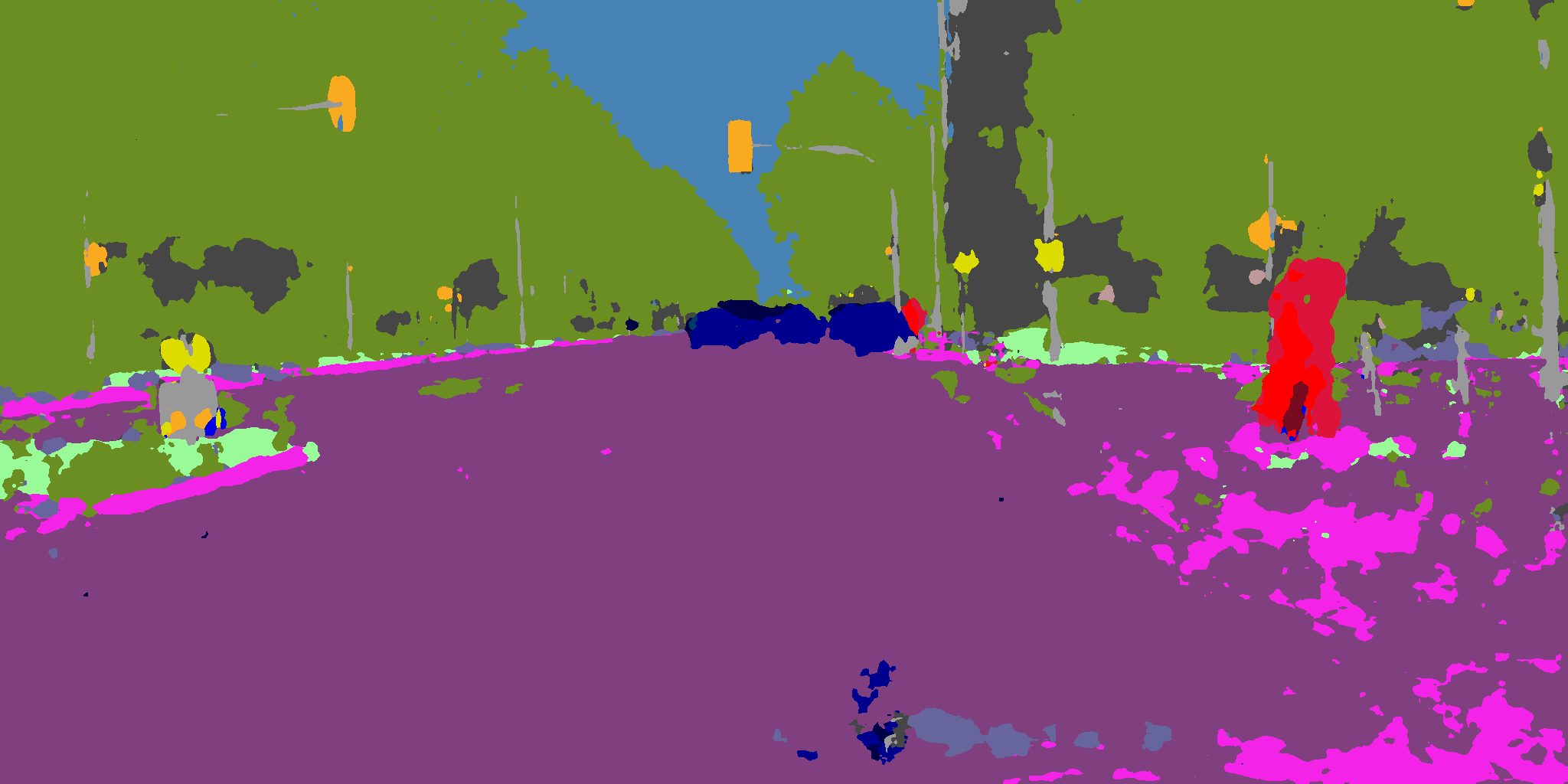
Figure 5: Qualitative results of zero-shot adaptation. (Columns 1-2) Input images and their ground truths; (Columns 3-4) Segmentation results of source-only and  PØDA models.

Real$\shortrightarrow$synthetic is an interesting though under-explored adaptation scenario. One potential application of real$\shortrightarrow$synthetic is for model validation in the industry, where some hazardous validations like driving accidents must be done in the virtual space. Here we test if our zero-shot mechanism can be also applied to this particular setting. Similarly, PØDA outperforms both baselines. Also in the reverse synthetic$\shortrightarrow$real setting, again our method performs the best. CLIPstyler undergoes almost $5\%$ drops in mIoU compared to source-only.

We argue on the simplicity of our method that only introduces minimal changes to the feature statistics, yet such changes are crucial for target adaptation. CLIPstyler, designed for style transfer, involves training an additional StyleNet with $\approx{}615$k parameters for synthesizing the stylized images. We base on the simplicity merit of PØDA to explain why it is more favorable than CLIPstyler for downstream tasks like semantic segmentation: the minimal statistics changes help avoiding significant drifts on the feature manifold which may otherwise result in unwanted errors. For comparison, it takes us $0.3$ seconds to augment one source feature, while stylizing an image with CLIPstyler takes $65$ seconds (as measured on one RTX 2080TI GPU).

Source	Target eval.	One-shot SM-PPM [56]	Zero-shot PØDA
CS	ACDC Night	13.07 / 14.60 ($\Delta$=1.53)	18.31 / 25.03  ($\Delta$=6.72)
	ACDC Snow	32.60 / 35.61  ($\Delta$=3.01)	39.28 / 43.90  ($\Delta$=4.62)
	ACDC Rain	29.78 / 32.23  ($\Delta$=2.45)	38.20 / 42.31  ($\Delta$=4.11)
GTA5	CS	30.48 / 39.32  ($\Delta$=8.84)	36.38 / 40.08  ($\Delta$=3.70)

Table 3: Comparison with SM-PPM. Semantic segmentation performance (mIoU%) for source / adapted models, and gain provided by adaptation ($\Delta$ in mIoU). For adaptation, SM-PPM (ResNet-101 DeepLabv2) has access to one target image, while PØDA (ResNet-50 DeepLabv3+) leverages a target prompt and a text encoder.

We show in Fig. 5 qualitative examples of predictions from source-only and PØDA models. We report class-wise performance in Supplementary Material.

Method	ACDC Night	ACDC Snow	ACDC Rain	GTA5
Source only	18.31 $\pm$0.00	39.28 $\pm$0.00	38.20 $\pm$0.00	39.59 $\pm$0.00
Trg	“driving at night”	“driving in snow”	“driving under rain”	“driving in a game”
	25.03 $\pm$0.48	43.90 $\pm$0.53	42.31 $\pm$0.55	41.07 $\pm$0.48
$\longleftarrow$Irrelevant ChatGPT-generated Relevant $\longrightarrow$	c“operating a
vehicle
after sunset”	c“operating a
vehicle in
snowy conditions”	c“operating a
vehicle in
wet conditions”	c“piloting a
vehicle in
a virtual world”
	24.38 $\pm$0.37	44.33 $\pm$0.36	42.21 $\pm$0.47	41.25 $\pm$0.40
	c“driving during
the nighttime
hours”	c“driving on
snow-covered
roads”	c“driving on
rain-soaked
roads”	c“controlling a car
in a digital
simulation”
	25.22 $\pm$0.64	43.56 $\pm$0.62	42.51 $\pm$0.33	41.19 $\pm$0.14
	c“navigating
the roads
in darkness”	c“piloting a
vehicle in
snowy terrain”	c“navigating
through rainfall
while driving”	c“maneuvering
a vehicle in a
computerized racing
experience”’
	24.73 $\pm$0.47	44.67 $\pm$0.18	41.11 $\pm$0.69	40.34 $\pm$0.49
	c“driving in
low-light
conditions”	c“driving in
wintry
precipitation”	c“driving in
inclement
weather”	c“operating
a transport
in a video game
environment”
	24.68 $\pm$0.34	43.11 $\pm$0.56	40.68 $\pm$0.37	41.34 $\pm$0.42
	c“travelling
by car
after dusk”	c“travelling
by car in
a snowstorm”	c“travelling by
car during
a downpour”	c“navigating a
machine through
a digital
driving simulation”
	24.89 $\pm$0.24	43.83 $\pm$0.17	42.05 $\pm$0.35	41.86 $\pm$0.10
	24.82 $\pm$0.00	43.90 $\pm$0.00	41.81 $\pm$0.00	41.18 $\pm$0.00
	c“mesmerizing northern lights display”
	20.05 $\pm$0.77	40.07 $\pm$0.66	38.43 $\pm$0.82	37.98 $\pm$0.31
	c“playful dolphins in the ocean”
	20.11 $\pm$0.31	39.87 $\pm$0.26	38.56 $\pm$0.58	37.05 $\pm$0.31
	c“breathtaking view from mountaintop”
	20.65 $\pm$0.33	42.08 $\pm$0.28	40.05 $\pm$0.52	40.09 $\pm$0.23
	c“cheerful sunflower field in bloom”
	21.10 $\pm$0.50	39.85 $\pm$0.68	40.09 $\pm$0.41	37.93 $\pm$0.55
	c“dramatic cliff overlooking the ocean”
	20.09 $\pm$0.98	38.20 $\pm$0.54	38.48 $\pm$0.37	37.57 $\pm$0.46
	c“majestic eagle in flight over mountains”
	20.70 $\pm$0.38	39.60 $\pm$0.27	40.38 $\pm$0.86	38.52 $\pm$0.21
	20.45 $\pm$0.00	39.95 $\pm$0.00	39.33 $\pm$0.00	38.19 $\pm$0.00

Table 4: Effect of prompts on PØDA. We show result for our $\mathsf{TrgPrompt}{}$ (top) as well as ChatGPT-generated relevant prompt (middle) and irrelevant prompt (bottom). Please refer to Sec. 4.3 for details. Best results (bold) are always obtained with relevant prompts for which mean mIoU (italic) also proves to be better.

Comparison to one-shot UDA (OSUDA). We also compare PØDA against SM-PPM [56], a state-of-the-art OSUDA method, see Tab. 3. The OSUDA setting allows the access to a single unlabeled target domain image for DA. In SM-PPM, this image is considered as an anchor point for target style mining. Using $5$ randomly selected target images, we trained, with each one, five models with different random seeds. The reported mIoUs are averaged over the 25 resulting models. We note that the absolute results of the two models are not directly comparable due to the differences in backbone (ResNet-101 in SM-PPM vs. ResNet-50 in PØDA) and in segmentation framework (DeepLabv2 in SM-PPM vs. DeepLabv3+ in PØDA). We thus analyze the improvement of each method over the corresponding naive source-only baseline while taking into account the source-only performance. We first notice that our source-only (CLIP ResNet) performs better than SM-PPM source-only (ImageNet pretrained ResNet), demonstrating the overall robustness of the frozen CLIP-based model. In Cityscapes$\shortrightarrow$ ACDC, both absolute and relative improvements of PØDA over source-only are greater than the ones of SM-PPM. Overall, PØDA exhibits on par or greater improvements over SM-PPM, despite the fact that our method is purely zero-shot.

Qualitative results on uncommon conditions. Figure 6 shows some qualitative results, training on Cityscapes, and adapting to uncommon conditions never found in datasets because they are either rare (sandstorm), dangerous (fire), or not labeled (old movie). For all, PØDA improves over source-only, which demonstrates its true benefit.

4.3 Ablation studies

$\mathsf{TrgPrompt}$ selection.  Using any meaningful descriptions of the target domain, one should obtain similar adaptation gain with PØDA. To verify this, we generate other relevant prompts by querying ChatGPT with Give me 5 prompts that have the same exact meaning as [PROMPT] using same prompts as in Tab. 2. Results in Tab. 4 show that adaptation gains are rather independent of the textual expression. Inversely, we query irrelevant prompts with Give me 6 random prompts of length from 3 to 6 words describing a random photo, which could result in negative transfer (See Tab. 4). By chance, small gains could occur; however we conjecture that such gains may originate from generalization by randomization rather than adaptation.

Input	Source-only	PØDA
$\mathsf{TrgPrompt}$ = “driving through fire”
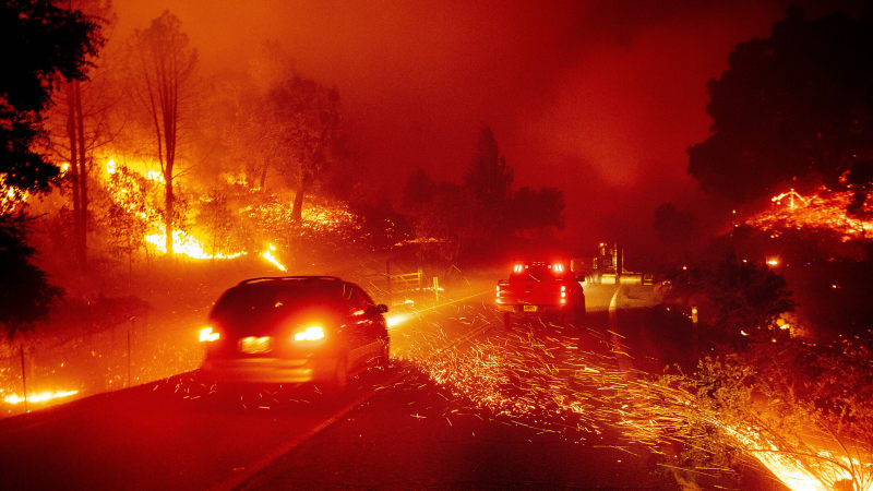
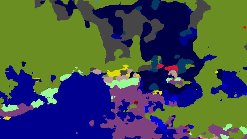
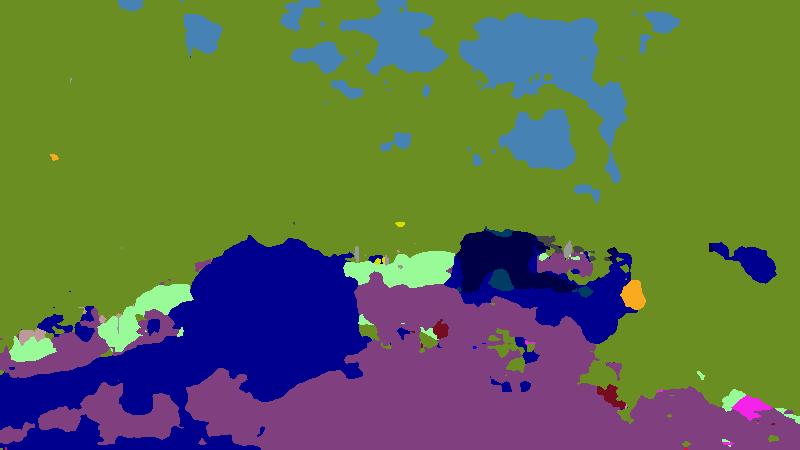
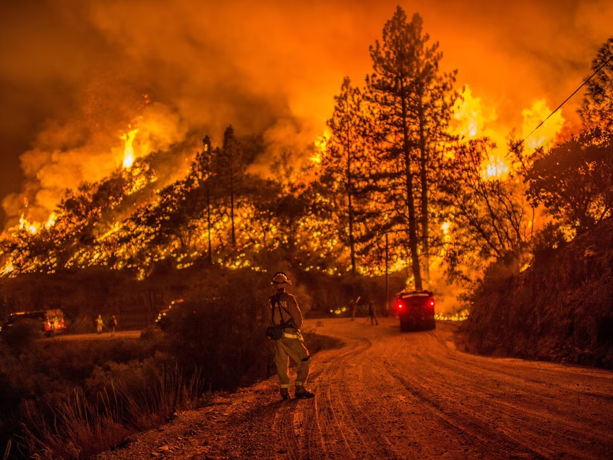
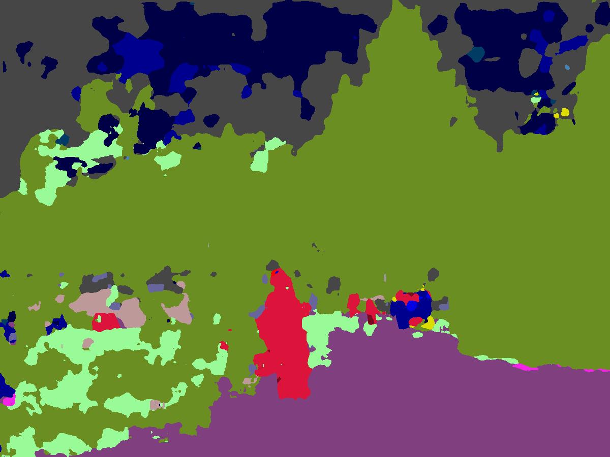
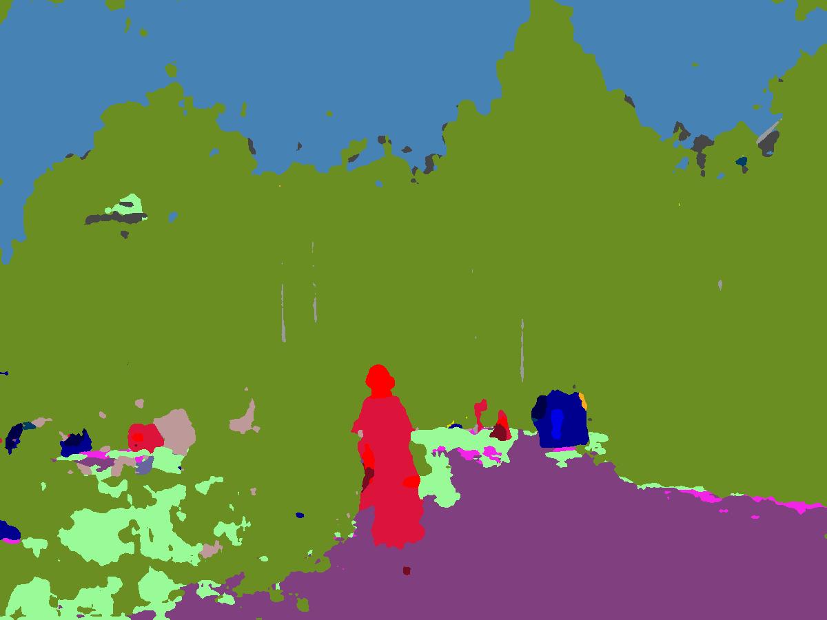
$\mathsf{TrgPrompt}$ = “driving in sandstorm”
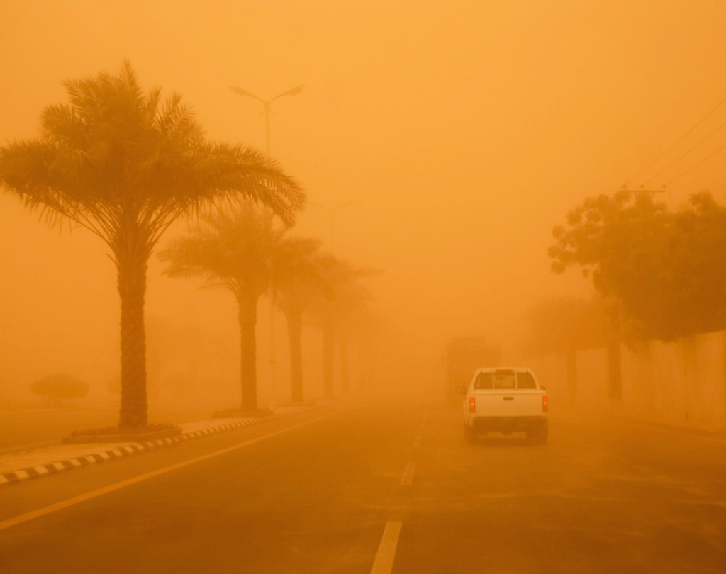
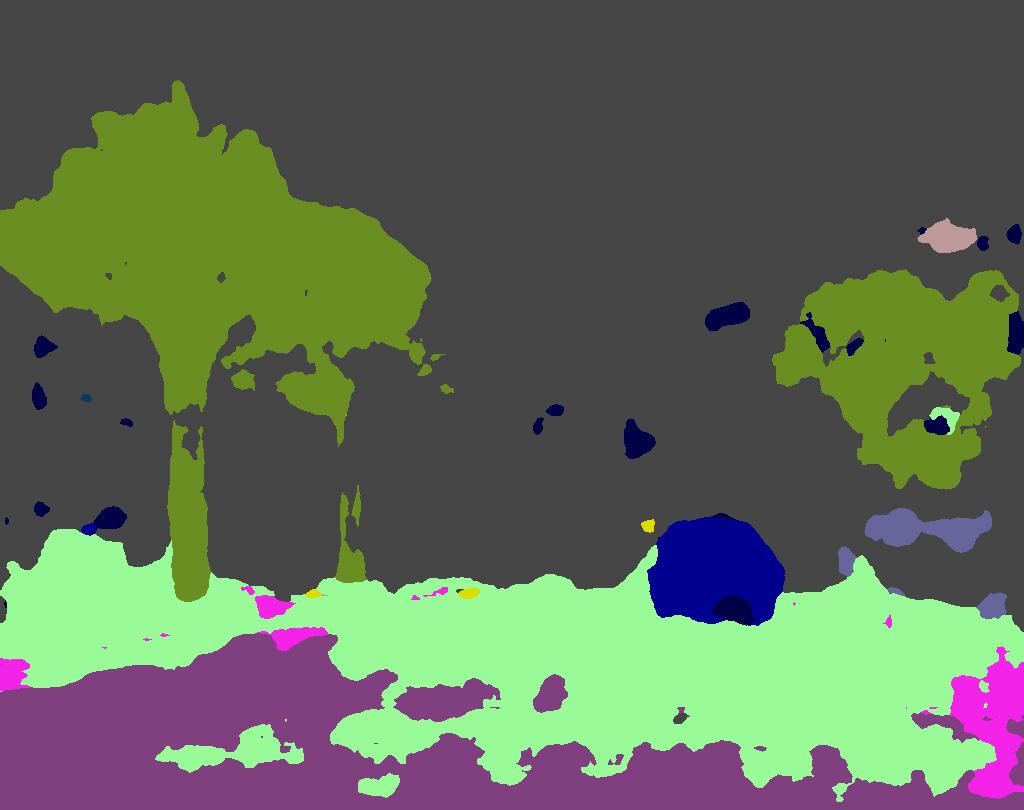
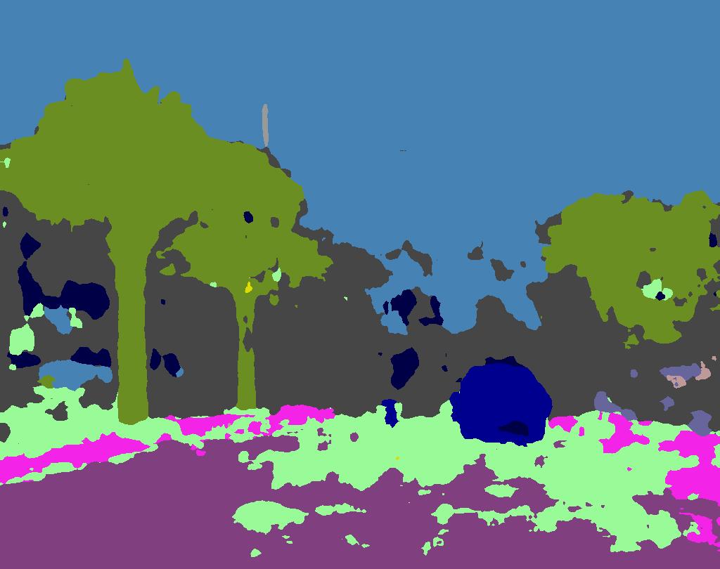
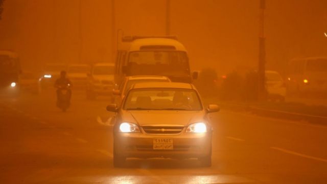
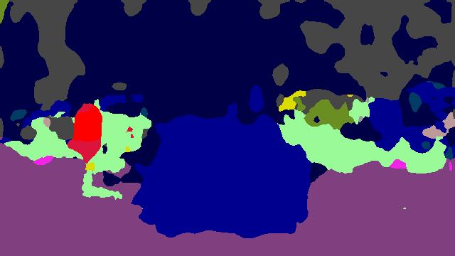
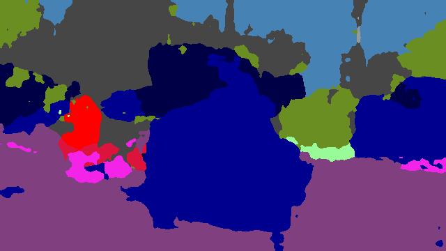
$\mathsf{TrgPrompt}$ = “driving in old movie”

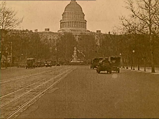
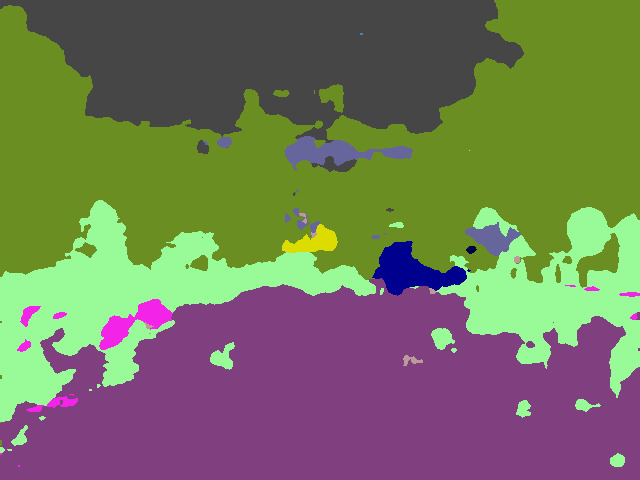
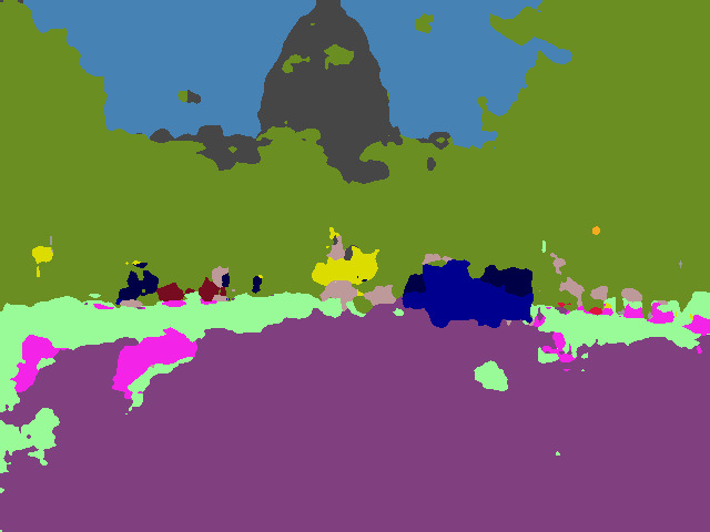
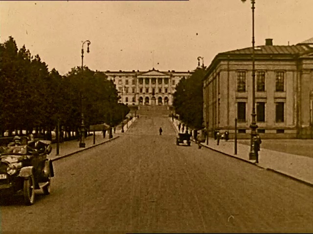
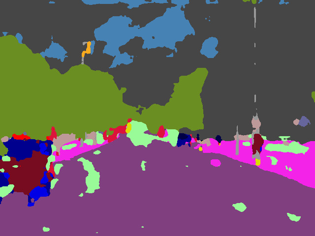
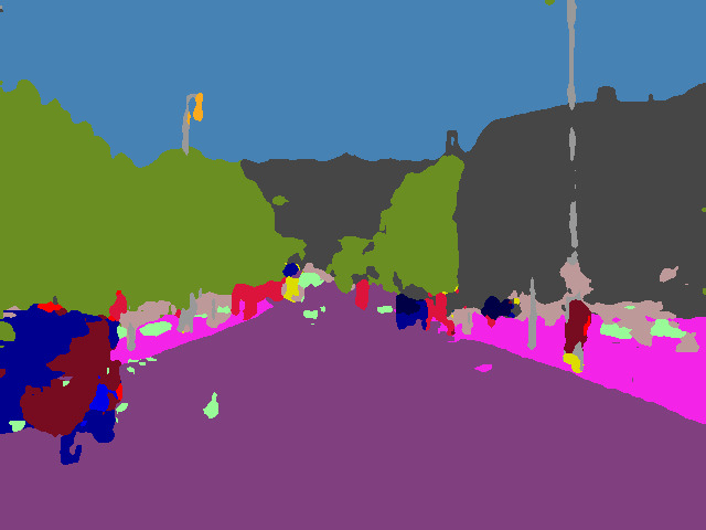
Figure 6: PØDA on uncommon conditions. Qualitative results here all use Cityscapes as source and PØDA uses $\mathsf{TrgPrompt}$.

Choice of features to augment.  DeepLabV3+ segmenter takes as inputs both low-level features from Layer1 and high-level features from Layer4. In PØDA, we only augment the Layer1 features and forward them through remaining layers 2-4 to obtain the Layer4 features. The input to the classifier is the concatenation of both. We study in Tab. 5 if one should augment other features in addition to the ones in Layer1: we observe the best performance with only Layer1 augmentation. We conjecture that it is important to preserve the consistency between the two inputs to the classifier, i.e., Layer4 features should be derived from the augmented one from Layer1.

Number of mined styles.  Our experiments use always $|{\mathcal{S}}_{\text{s}\shortrightarrow\text{t}}|=|{\mathcal{D}}_{\text{s}}|$ but we study the effect of changing the number $|{\mathcal{S}}_{\text{s}\shortrightarrow\text{t}}|$ of styles on the target domain performance. By performing ablation on CS$\shortrightarrow$Night with $|{\mathcal{S}}_{\text{s}\shortrightarrow\text{t}}|=$ 1, 10, 100, 1000, 2975 (i.e., $|{\mathcal{D}}_{\text{s}}|$), we obtain 16.00 $\pm$5.01, 22.04 $\pm$1.24, 23.90 $\pm$0.96, 24.27 $\pm$0.70, 25.03 $\pm$0.48 respectively. For $|{\mathcal{S}}_{\text{s}\shortrightarrow\text{t}}|<|{\mathcal{D}}_{\text{s}}|$, the styles are sampled randomly from ${\mathcal{D}}_{\text{s}}$ and results are reported in average on 5 different samplings. Interestingly, we observe that the variance decreases with the increase of $|{\mathcal{S}}_{\text{s}\shortrightarrow\text{t}}|$. Results also suggest that only few styles (e.g. $|{\mathcal{S}}_{\text{s}\shortrightarrow\text{t}}|=10$) could be sufficient for feature translation, similarly to few-shot image-to-image translation [39], though at the cost of higher variance.

Partial unfreezing of the backbone.  While our experiments use a frozen backbone due to the observed good out-of-distribution performance (Tab. 1), we highlight that during training only Layer1 must be frozen to preserve its activation space where augmentations are done; the remaining three layers could be optionally fine-tuned. Results in  Tab. 6 show that freezing the whole backbone (i.e., Layer1-4) achieves the best results. In all cases, PØDA consistently improves the performance over source-only.

Layer1	Layer2	Layer3	Layer4	ACDC Night
✓	✗	✗	✗	25.03 $\pm$0.48
✓	✓	✗	✗	23.43 $\pm$0.51
✓	✗	✓	✗	22.93 $\pm$0.53
✓	✗	✗	✓	21.05 $\pm$0.55

Table 5: Impact of selected layers for augmentation. Performance (mIoU) of PØDA’s day$\shortrightarrow$night adaptation for different choices of ResNet layers for feature augmentation. In addition to augmenting features of Layer1 (Row 1), one can augment Layer2 or Layer3 features (Rows 2-3), or of Layer4 directly (Row 4).

Method	Night	Snow	Rain	GTA5
src-only*	18.31 $\pm$0.00	39.28 $\pm$0.00	38.20 $\pm$0.00	39.59 $\pm$0.00
PØDA*	25.03 $\pm$0.48	43.90 $\pm$0.53	42.31 $\pm$0.55	41.07 $\pm$0.48
src-only (Layer1 2744)	9.60 $\pm$0.00	30.99 $\pm$0.00	30.89 $\pm$0,00	29.38 $\pm$0.00
PØDA (Layer1 2744)	19.43 $\pm$0.69	37.80 $\pm$2.65	40.71 $\pm$1.06	39.09 $\pm$1.23

Table 6: PØDA when freezing (2744) only Layer1. Both models with *, reported in Tab. 2, freeze the whole backbone Layer1-4.

Method	Night	Snow	Rain	GTA5
Source-only	18.31 $\pm$0.00	39.28 $\pm$0.00	38.20 $\pm$0.00	39.59 $\pm$0.00
Source-only-G	21.07 $\pm$0.00	42.84 $\pm$0.00	42.38 $\pm$0.00	41.54 $\pm$0.00
PØDA-G	24.86 $\pm$0.70	44.34 $\pm$0.36	43.17 $\pm$0.63	41.73 $\pm$0.39
PØDA-G+style-mix	24.18 $\pm$0.23	44.46 $\pm$0.34	43.56 $\pm$0.46	42.98 $\pm$0.12

Table 7: Generalization with PØDA. Source-only-G model is enhanced with a domain generalization technique. Training PØDA from Source-only-G (‘PØDA-G’) brings improvements. ‘style-mix’: style mixing as in [56].

4.4 Further discussion

Generalization with PØDA.  Inspired by the observation that some unrelated prompts improve performance on target domains (see Tab. 4), we study how PØDA can benefit from general style augmentation. First, we coin “Source-only-G” the generalized source-only model where we augment features by shifting the per-channel $(\bm{\mu},\bm{\sigma})$ with Gaussian noises sampled for each batch of features, such that the signal to noise ratio is 20 dB. This source-only variant takes inspiration from [15] where simple perturbations of feature channel statistics could help achieve SOTA generalization performance in object detection. Tab. 7 shows that Source-only-G always improves over Source-only, demonstrating a generalization capability. When applying our zero-shot adaptation on Source-only-G (denoted “PØDA-G”), target performance again improves – always performing best on the desired target. Performance is further boosted by the style mixing strategy used in [56], i.e. source and augmented features statistics being linearly mixed.

Effect of priors.  We now discuss existing techniques that approach zero-shot DA with different priors, revealing the potential combinations of different orthogonal methods. In Tab. 8, we report zero-shot results of CIConv [26] using physics priors, compared against CLIPstyler and PØDA, which use textual priors, i.e., prompts. We also include the one-shot SM-PPM [56] model as the single target sample it requires can be considered as a prior. CIConv, a dedicated physics-inspired layer, is proven effective in enhancing backbone robustness on night scenes. The layer could be straightforwardly included in the CLIP image encoder to achieve the same effect. Albeit interesting, this combination would however require extremely high computational resources to re-train a CLIP variant equipped with CIConv. We leave open such a combination, as well as others like (i) combining image-level (CLIPstyler) and feature-level augmentation (PØDA) or (ii) additionally using style information from one target sample (like in SM-PPM) to help in guiding better the feature augmentation.

Other architectures.  We show in Tab. 9 consistent gains brought by PØDA using new backbone (RN101 [18]) and segmenter (semantic FPN [24]).

Method	Prior	ACDC Night
CIConv* [26]	physics	30.60 / 34.50 ($\Delta$=3.90)
SM-PPM [56]	1 target image	13.07 / 14.60 ($\Delta$=1.53)
CLIPstyler [25]	1 prompt	18.31 / 21.38 ($\Delta$=3.07)
PØDA	1 prompt	18.31 / 25.03 ($\Delta$=6.72)

* Results of CIConv are on DarkZurich, a subset of ACDC Night [45].

Table 8: Effect of different priors for zero-shot/one-shot adaptation. We report mIoU% for source-only / adapted models, and gain brought by adaptation ($\Delta$ in mIoU). Note that [26, 56] use a deeper backbone making results not directly comparable.

Backbone	Method	Night	Snow	Rain	GTA5
Sem. FPN	src-only	18.10 $\pm$0.00	35.75 $\pm$0.00	36.07 $\pm$0.00	40.67 $\pm$0.00
	PØDA	21.48 $\pm$0.15	39.55 $\pm$0.13	38.34 $\pm$0.29	41.59 $\pm$0.24
DLv3+	src-only	22.17 $\pm$0.00	44.53 $\pm$0.00	42.53 $\pm$0.00	40.49 $\pm$0.00
	PØDA	26.54 $\pm$0.12	46.71 $\pm$0.43	46.36 $\pm$0.20	43.17 $\pm$0.13

Table 9: PØDA with different architectures. Backbones are RN50 for Semantic FPN (‘Sem. FPN’) and RN101 for DeepLabV3+ (‘DLv3+’).

5 PØDA for other tasks

PØDA operates at the features level, which makes it task-agnostic. We show in the following the effectiveness of our method for object detection and image classification.

PØDA for Object Detection.  We report in Tab. 10 some results when straightforwardly applying PØDA to object detection. Our Faster-RCNN [41] models, initialized with two backbones, are trained on two source datasets, either Cityscapes or the Day-Clear split in Diverse Weather Dataset (DWD) [55]. We report adaptation results on Cityscapes-Foggy [44] and four other conditions in DWD. For zero-shot feature augmentation in PØDA, we use simple prompts and take the default optimization parameters in previous experiments.  PØDA obtains on par or better results than UDA methods [8, 42] (which use target images) and domain generalization methods [15, 55, 49]. We also experimented with YOLOF [7] for object detection in CS$\shortrightarrow$Foggy; PØDA reaches $35.4\%$, improving $1.5\%$ from the source-only model. These results open up potential combinations of PØDA with generalization techniques like [15] and [49] for object detection.

		CS$\shortrightarrow$ CS Foggy	DWD-Day Clear $\shortrightarrow$
Method	Target		Night Clear	Dusk Rainy	Night Rainy	Day Foggy
DA-Faster [8]	✓	32.0	-	-	-	-
ViSGA [42]	✓	43.3	-	-	-	-
NP+ [15]	✗	46.3	-	-	-	-
S-DGOD [55]	✗	-	36.6	28.2	16.6	33.5
CLIP The Gap [49]	✗	-	36.9	32.3	18.7	38.5
PØDA	✗	47.3	43.4	40.2	20.5	44.4

Table 10: PØDA for object detection (mAP%). For Cityscapes$\shortrightarrow$Cityscapes-Foggy adaptation, the backbone is ResNet-50, while it is ResNet-101 for adaption from DWD-Day-Clear to other conditions in DWD.

PØDA for Image Classification. We show that PØDA can be also applied for image classification. We use the same augmentation strategy to adapt a linear probe on top of CLIP-RN50 features. In a first experiment we train a linear classifier on the features of CUB-200 dataset [51] of 200 real bird species; we then perform zero-shot adaptation to classify bird paintings of CUB-200-Paintings dataset [53] using the single prompt “Painting of a bird”. In our second experiment, we address the color bias in Colored MNIST [1]; while for training, even and odd digits are colored red and blue respectively, the test digits are randomly colored. We augment training digit features using the “Blue digit” and “Red digit” prompts for even and odd digits respectively, and create a separate set for each one to prevent styles from leaking, i.e. to avoid trivially using “red” styles coming from even digits to augment odd digits features and vice versa. Results in Tab. 11 show that PØDA significantly improves over the source-only models.

Method	CUB-200 paintings	Colored MNIST
src-only	28.90 $\pm$0.00	55.83  $\pm$0.00
PØDA	30.91 $\pm$0.69	64.16 $\pm$0.41

Table 11: PØDA for image classification (acc%). The backbone is ResNet-50, and a linear classifier is fit on top of the features. The source domains are CUB-200 (real bird images) and colored MNIST with color bias, in second and third columns respectively.

6 Conclusion

In this work, we leverage the powerful zero-shot ability of the CLIP model to make possible a new challenging task of domain adaptation using prompts. We propose a cost-effective feature augmentation mechanism that adjusts the style-specific statistics of source features to synthesize augmented features in the target domain, guided by domain prompts in natural language. Extensive experiments have proven the effectiveness of our framework for semantic segmentation in particular. They also show its applicability to other tasks and various backbones. Our line of research aligns with the collective efforts of the community to leverage large-scale pre-trained models (so-called “foundation models” [3]) for data- and label-efficient training of perception models for real-world applications.

Acknowledgment.  This work was partially funded by French project SIGHT (ANR-20-CE23-0016). The authors also thank Ivan Lopes and Fabio Pizzati for their kind proofreading.

Appendix A Overall pseudo-code of PØDA

Algorithm 2 presents the high-level pseudo-code of PØDA: from source-only training as model initialization, to prompt-driven feature augmentation, to zero-shot model adaptation.

Appendix B Experimental details

Feature augmentation. PIN operates on image features. For augmentation, we optimize ($\bm{\mu},\bm{\sigma}$) of source feature map ${\mathbf{f}}_{\text{s}}$; it is done in batches for the sake of speed. We fix the batch size $b=16$ and the learning rate $lr=1.0$.

Style mixing. In the discussion of PØDA (Sec. 4.4 and Tab. 7), we presented the performance gains that style-mixing [56] brings to our method in three settings. By randomly mixing original and augmented statistics, we introduce certain perturbations to the final augmented features. The mixed statistics $\bm{\mu}_{\text{mix}},\bm{\sigma}_{\text{mix}}$ are given by:

$$\bm{\mu}_{\text{mix}}=\bm{\alpha}{\bm{\mu}}_{\text{t}}+(1-\bm{\alpha}){\bm{\mu}}_{\text{s}}\,,$$ (4)

$$\bm{\sigma}_{\text{mix}}=\bm{\alpha}{\bm{\sigma}}_{\text{t}}+(1-\bm{\alpha}){\bm{\sigma}}_{\text{s}}\,,$$ (5)

where $\bm{\alpha}\in\mathbb{R}^{c}$ are per-channel mixing weights uniformly sampled in $[0,1]$, similarly to [56]; multiplications are element-wise. Finally, the augmented features are computed as follows:

$$\mathbf{f}_{\text{s}\shortrightarrow\text{t}}=\texttt{PIN}({\mathbf{f}}_{\text{s}},\bm{\mu}_{\text{mix}},\bm{\sigma}_{\text{mix}}),$$ (6)

with prompt-driven instance normalization PIN defined in Eq. 2.

Appendix C Additional experiments

Effect of style mining initialization. In our feature optimization step, we initialize $(\bm{\mu},\bm{\sigma})$ with $(\mu({\mathbf{f}}_{\text{s}}),\sigma({\mathbf{f}}_{\text{s}}))$. In Tab. 12, we report results using different initialization strategies. Starting from pre-defined or random initialization, instead of from original statistics, degrades badly the performance. As we do not use any regularization term in the CLIP cosine distance loss, we argue that initializing the optimized statistics with those of the source images is a form of regularization, favoring augmented features in a neighborhood of ${\bar{\mathbf{f}}}_{\text{s}}$ and better preserving the semantics.

Input : Source dataset ${\mathcal{D}}_{\text{s}}=\{({\mathbf{x}}_{\text{s}},{\mathbf{y}}_{\text{s}})\}$

CLIP encoders $E_{\text{img}}$ and $E_{\text{txt}}$

Target domain description $\mathsf{TrgPrompt}$

Feature backbone $M_{\text{feat}}\xleftarrow{}E_{\text{img}}$

Source model: $M=(M_{\text{feat}},M_{\text{cls}})$

Result: Target-adapted model $M^{\prime}=(M_{\text{feat}},M^{\prime}_{\text{cls}})$

// Initialization

1 $\mathsf{TrgEmb}=E_{\text{txt}}(\mathsf{TrgPrompt})$

2 $M_{\text{cls}}\leftarrow\textnormal{{train}}(M_{\text{cls}},{\mathcal{D}}_{\text{s}})$ $\triangleright$ source-only training

// Feature Augmentation

3 ${\mathcal{F}}_{\text{s}}\leftarrow\textnormal{{feat-ext}}(M_{\text{feat}},\{{\mathbf{x}}_{\text{s}}\})$

4 ${\mathcal{S}}_{\text{s}\shortrightarrow\text{t}}\leftarrow\texttt{augment}({\mathcal{F}}_{\text{s}},\mathsf{TrgEmb})$

// Adaptation

5 $M^{\prime}_{\text{cls}}\leftarrow\textnormal{{fine-tune}}(M_{\text{cls}},{\mathcal{F}}_{\text{s}},{\mathcal{S}}_{\text{s}\shortrightarrow\text{t}},\{{\mathbf{y}}_{\text{s}}\})$ $\triangleright$ fine-tuning

Algorithm 2 Prompt-driven Zero-shot DA

$\bm{\mu}^{0}$	$\bm{\sigma}^{0}$	mIoU
$\mu({\mathbf{f}}_{\text{s}})$	$\sigma({\mathbf{f}}_{\text{s}})$	25.03 $\pm$0.48
$\mathbf{0}$	$\mathbf{1}$	8.59 $\pm$0.82
$\sim\mathcal{N}(\mathbf{0},\mathbf{I})$	$\sim\mathcal{N}(\mathbf{0},\mathbf{I})$	6.80 $\pm$0.92

Table 12: Effect of style initialization. Performance (in mIoU) of PØDA on ACDC-Night val set (Cityscapes as source), with different style statistics initializations. Starting from source images’ statistics works substantially better.

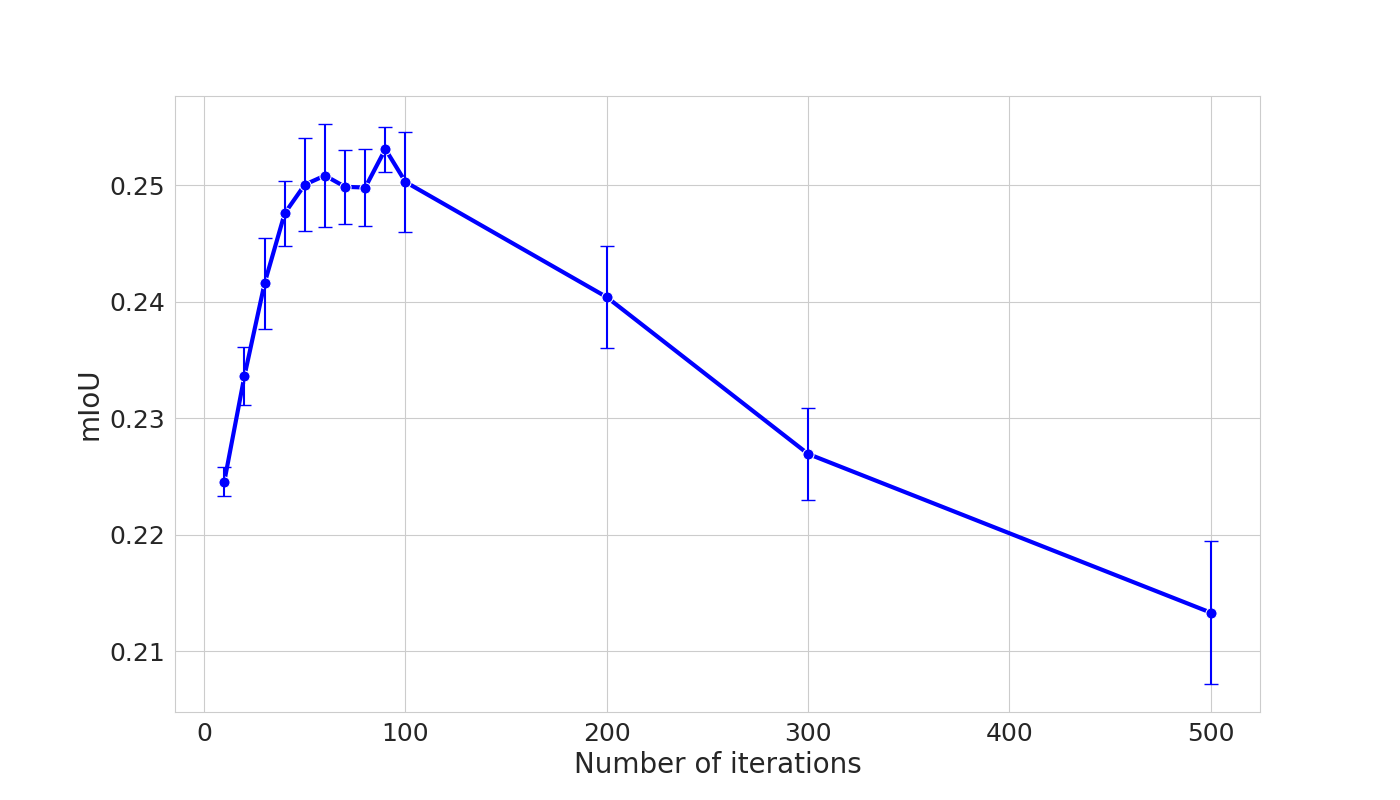
Figure 7: Effect of the number of optimization iterations. Performance (mIoU %) of PØDA adaptation from Cityscapes to ACDC-Night as a function of the number of statistics optimization iterations. The values are averages over 5 runs and the bars represent the standard deviation.

Optimization steps. In all our experiments, $100$ iterations of optimization are performed for each batch of source features. We show in Fig. 7 the effect of the total number of iterations. We see an inflection point at around 80-100 iterations. Using few iterations is not sufficient for style alignment. Above $100$, we also observe a performance drop. We refer to [25] and argue for the “over-stylization” problem in this case.

Diversity of optimized statistics. To verify that the statistics — optimized for the same number of iterations with the same $\mathsf{TrgPrompt}$ but from different starting anchor points $\bar{{\mathbf{f}}_{\text{s}}}$ — are diverse, we show in Fig. 8 the boxplots of optimized parameters on the first $20$ channels of ${\mathbf{f}}_{\text{s}\shortrightarrow\text{t}}$ (for prompt “driving at night”).

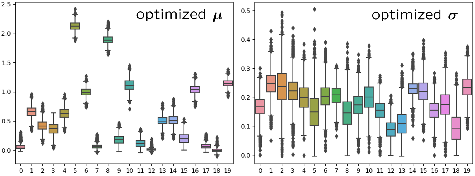
Figure 8: Per-channel optimized statistics. Distributions of the first $20$ channels of the optimized statistics of $\bm{\mu}$ (Left) and $\bm{\sigma}$ (Right). Each boxplot shows the interquartile range (IQR) that contains 50% of the data: Its bottom and top edges delimit the first and third quartiles respectively. The horizontal line inside the box denotes the data median. The whiskers extend from the edges of the box to the furthest point within $1.5$ times the IQR, in each direction. Outlier points beyond these limits are individually plotted (diamonds).

Training from scratch on augmented features. In PØDA, we start with a source-only trained model (Algorithm 2, line 2) then we fine-tune it on augmented features (Algorithm 2, line 5). This is the general setting for domain adaptation. However, since our method performs domain adaptation under the assumption of label preservation, we also experimented training the model from scratch on augmented features. The results (Tab. 13) show the importance of the first, source-only training step.

Method	Night	Snow	Rain	GTA5
PØDA no src pretrain	22.46	36.73	39.70	39.57
PØDA	25.03	43.90	42.31	41.07

Table 13: Importance of source-only pre-training. Semantic segmentation performance (mIoU %) of PØDA vs. its variant without source-only training, when adapting from Cityscapes to ACDC Nigt/Snow/Rain and to GTA5.

Testing PØDA on other datasets.  PØDA does not use target datasets at any point in training. Although there is no reason for the improvements observed to be specific for the datasets we test on, we show in Tab. 14 the performance of the model adapted using “driving at night” on two additional night-time driving scenes datasets:

• Nighttime Driving [13] test set, which consists of 50 annotated images of night driving scenes, with resolution of $1920\times 1080$.

• NightCity [47], which is a large dataset of 4297 night-time driving scenes collected from many cities around the world; We tested on the validation/testing set, which consists of 1299 images of resolution $1024\times 512$.

	ACDC Night	Nighttime Driving [13]	NightCity [47]
Source-only	18.31 $\pm$0.00	29.61 $\pm$0.00	25.63 $\pm$0.00
PØDA	25.03 $\pm$0.48	33.98 $\pm$0.61	28.90 $\pm$0.61

Table 14: PØDA at night. Segmentation performance (mIoU %) of PØDA adapted from Cityscapes to nighttime with $\mathsf{TrgPrompt}$ = “driving at night”, on three different night-time driving datasets.

Appendix D Class-wise performance

We report class-wise IoUs in Tab. 15.

Source	Target eval.	Method	road	sidewalk	building	wall	fence	pole	traffic light	traffic sign	vegetation	terrain	sky	person	rider	car	truck	bus	train	motorcycle	bicycle	mIoU%
CS	$\mathsf{TrgPrompt}$ = “driving at night”
	ACDC Night	source-only	70.42	18.32	43.83	6.11	17.08	23.52	24.51	19.76	39.74	6.11	0.78	21.62	8.96	23.08	2.53	0.00	3.27	8.42	9.87	18.31 $\pm$0.00
		CLIPstyler	73.96	23.26	42.16	3.31	7.21	35.49	23.34	19.01	45.41	8.81	27.87	21.06	8.48	38.17	1.84	0.00	11.54	10.38	4.89	21.38 $\pm$0.36
		PØDA	77.54	26.90	42.71	13.51	21.36	33.52	23.70	21.73	39.91	9.51	19.40	28.80	11.85	50.89	10.14	0.00	20.76	8.76	14.50	25.03 $\pm$0.48
	$\mathsf{TrgPrompt}$ = “driving in snow”
	ACDC snow	source-only	70.47	23.50	63.80	17.96	27.36	38.52	56.26	45.00	83.00	10.75	83.65	47.73	0.72	61.42	21.87	5.90	21.58	35.83	31.01	39.28 $\pm$0.00
		CLIPstyler	74.29	31.25	69.17	15.21	25.21	36.83	44.79	42.56	76.87	11.07	91.48	53.23	0.13	67.66	23.88	9.14	36.48	42.67	28.76	41.09 $\pm$0.17
		PØDA	75.40	34.61	75.22	26.77	27.34	35.20	52.68	44.37	82.01	14.16	93.72	50.51	0.99	69.11	26.64	2.72	46.98	42.64	33.09	43.90 $\pm$0.53
	$\mathsf{TrgPrompt}$ = “driving under rain”
	ACDC rain	source-only	74.10	31.98	63.07	15.08	23.92	41.31	50.12	44.43	79.93	22.07	87.45	47.99	4.39	68.92	10.35	18.52	13.64	7.03	21.58	38.20 $\pm$0.00
		CLIPstyler	73.71	36.09	68.91	3.77	16.99	36.94	39.75	36.44	78.21	20.64	91.79	40.34	9.65	74.54	13.16	20.33	12.73	14.06	18.26	37.17 $\pm$0.10
		PØDA	76.60	38.52	78.01	15.02	22.53	40.33	45.39	41.40	86.85	37.97	96.46	50.39	6.35	74.19	19.19	7.98	22.06	21.04	23.65	42.31 $\pm$0.55
	$\mathsf{TrgPrompt}$ = “driving in a game”
	GTA5	source-only	68.72	22.65	78.79	36.81	17.31	39.66	39.33	14.84	72.61	22.53	87.31	57.50	26.14	74.29	44.57	20.45	0.00	18.30	10.35	39.59 $\pm$0.00
		CLIPstyler	73.06	29.89	77.86	25.50	11.69	39.72	35.88	24.04	67.38	12.75	88.77	46.58	33.38	72.03	42.79	11.12	0.00	28.84	14.61	38.73 $\pm$0.16
		PØDA	73.93	22.69	78.82	37.52	14.17	36.97	33.14	17.34	72.44	26.22	88.85	62.69	37.04	74.33	43.03	11.91	0.00	35.33	13.91	41.07 $\pm$0.48
	$\mathsf{TrgPrompt}$ = “driving”
GTA5	CS	source-only	58.97	20.92	72.84	16.53	24.58	31.37	34.77	23.62	82.12	17.04	66.28	63.46	14.72	81.27	20.83	17.19	4.68	20.57	19.56	36.38 $\pm$0.00
		CLIPstyler	66.70	23.63	64.12	5.08	3.66	20.67	19.31	18.10	81.68	12.36	81.04	54.64	0.52	73.47	20.65	22.30	4.03	15.79	10.73	31.50 $\pm$0.21
		PØDA	84.34	36.73	79.43	18.33	16.54	36.93	38.45	33.81	82.44	19.14	75.90	62.65	16.47	75.48	15.68	19.57	11.28	16.53	21.76	40.08 $\pm$0.52

Table 15: Zero-shot domain adaptation in semantic segmentation. Performance (mIoU%) of PØDA compared against CLIPstyler [25] and source-only baseline. Results are grouped by source domain and target domain with associated $\mathsf{TrgPrompt}$. CS stands for Cityscapes [11]. This table provides details of the main results in Tab. 2.

Appendix E PØDA for Object Detection

Here, we share the implementation details for our object detection experiments (Sec. 5 and Tab. 10). We used the implementation of Faster R-CNN [41] from the MMDetection library. With Cityscapes as source dataset, we trained all models for $8$ epochs using the SGD optimizer with $0.9$ momentum and $1\text{e}{-4}$ weight decay. The initial learning rate $lr$ is set as $1\text{e}{-2}$ and is dropped by a factor of 10 after the $7$th epoch; the same $lr$ scheme is used in source only and PØDA trainings. With Day-Sunny split of the DWD dataset as source, models are trained for $20$ epochs using a similar SGD optimizer. When training on source, the learning rate starts at $1\text{e}{-3}$ and drops at the $9$th epoch to $1\text{e}{-4}$; in PØDA training, the learning rate is ten times less.

References

- [1] Martin Arjovsky, Léon Bottou, Ishaan Gulrajani, and David Lopez-Paz. Invariant risk minimization. arXiv preprint arXiv:1907.02893, 2019.
- [2] Shai Ben-David, John Blitzer, Koby Crammer, Alex Kulesza, Fernando Pereira, and Jennifer Wortman Vaughan. A theory of learning from different domains. ML, 2010.
- [3] Rishi Bommasani, Drew A Hudson, Ehsan Adeli, Russ Altman, Simran Arora, Sydney von Arx, Michael S Bernstein, Jeannette Bohg, Antoine Bosselut, Emma Brunskill, et al. On the opportunities and risks of foundation models. arXiv preprint arXiv:2108.07258, 2021.
- [4] Léon Bottou. Large-scale machine learning with stochastic gradient descent. In COMPSTAT, 2010.
- [5] Liang-Chieh Chen, George Papandreou, Iasonas Kokkinos, Kevin Murphy, and Alan L Yuille. Deeplab: Semantic image segmentation with deep convolutional nets, atrous convolution, and fully connected crfs. IEEE T-PAMI, 2017.
- [6] Liang-Chieh Chen, Yukun Zhu, George Papandreou, Florian Schroff, and Hartwig Adam. Encoder-decoder with atrous separable convolution for semantic image segmentation. In ECCV, 2018.
- [7] Qiang Chen, Yingming Wang, Tong Yang, Xiangyu Zhang, Jian Cheng, and Jian Sun. You only look one-level feature. In CVPR, 2021.
- [8] Yuhua Chen, Haoran Wang, Wen Li, Christos Sakaridis, Dengxin Dai, and Luc Van Gool. Scale-aware domain adaptive faster r-cnn. IJCV, 2021.
- [9] Bowen Cheng, Maxwell D. Collins, Yukun Zhu, Ting Liu, Thomas S. Huang, Hartwig Adam, and Liang-Chieh Chen. Panoptic-deeplab: A simple, strong, and fast baseline for bottom-up panoptic segmentation. In CVPR, 2020.
- [10] Niv Cohen, Rinon Gal, Eli A Meirom, Gal Chechik, and Yuval Atzmon. “this is my unicorn, fluffy”: Personalizing frozen vision-language representations. In ECCV, 2022.
- [11] Marius Cordts, Mohamed Omran, Sebastian Ramos, Timo Rehfeld, Markus Enzweiler, Rodrigo Benenson, Uwe Franke, Stefan Roth, and Bernt Schiele. The cityscapes dataset for semantic urban scene understanding. In CVPR, 2016.
- [12] Guillaume Couairon, Asya Grechka, Jakob Verbeek, Holger Schwenk, and Matthieu Cord. Flexit: Towards flexible semantic image translation. In CVPR, 2022.
- [13] Dengxin Dai and Luc Van Gool. Dark model adaptation: Semantic image segmentation from daytime to nighttime. In ITSC, 2018.
- [14] Patrick Esser, Robin Rombach, and Bjorn Ommer. Taming transformers for high-resolution image synthesis. In CVPR, 2021.
- [15] Qi Fan, Mattia Segu, Yu-Wing Tai, Fisher Yu, Chi-Keung Tang, Bernt Schiele, and Dengxin Dai. Towards robust object detection invariant to real-world domain shifts. In ICLR, 2023.
- [16] Rinon Gal, Or Patashnik, Haggai Maron, Gal Chechik, and Daniel Cohen-Or. StyleGAN-NADA: CLIP-guided domain adaptation of image generators. In SIGGRAPH, 2022.
- [17] Yaroslav Ganin, Evgeniya Ustinova, Hana Ajakan, Pascal Germain, Hugo Larochelle, François Laviolette, Mario Marchand, and Victor Lempitsky. Domain-adversarial training of neural networks. JMLR, 2016.
- [18] Kaiming He, Xiangyu Zhang, Shaoqing Ren, and Jian Sun. Deep residual learning for image recognition. In CVPR, 2016.
- [19] Judy Hoffman, Eric Tzeng, Taesung Park, Jun-Yan Zhu, Phillip Isola, Kate Saenko, Alexei Efros, and Trevor Darrell. Cycada: Cycle-consistent adversarial domain adaptation. In ICML, 2018.
- [20] Xun Huang and Serge Belongie. Arbitrary style transfer in real-time with adaptive instance normalization. In ICCV, 2017.
- [21] Krishna Murthy Jatavallabhula, Alihusein Kuwajerwala, Qiao Gu, Mohd Omama, Tao Chen, Shuang Li, Ganesh Iyer, Soroush Saryazdi, Nikhil Keetha, Ayush Tewari, et al. Conceptfusion: Open-set multimodal 3d mapping. arXiv preprint arXiv:2302.07241, 2023.
- [22] Chao Jia, Yinfei Yang, Ye Xia, Yi-Ting Chen, Zarana Parekh, Hieu Pham, Quoc Le, Yun-Hsuan Sung, Zhen Li, and Tom Duerig. Scaling up visual and vision-language representation learning with noisy text supervision. In ICML, 2021.
- [23] Tero Karras, Samuli Laine, and Timo Aila. A style-based generator architecture for generative adversarial networks. In CVPR, 2019.
- [24] Alexander Kirillov, Ross Girshick, Kaiming He, and Piotr Dollár. Panoptic feature pyramid networks. In CVPR, 2019.
- [25] Gihyun Kwon and Jong Chul Ye. Clipstyler: Image style transfer with a single text condition. In CVPR, 2022.
- [26] Attila Lengyel, Sourav Garg, Michael Milford, and Jan C van Gemert. Zero-shot day-night domain adaptation with a physics prior. In ICCV, 2021.
- [27] Boyi Li, Kilian Q Weinberger, Serge Belongie, Vladlen Koltun, and René Ranftl. Language-driven semantic segmentation. In ICLR, 2022.
- [28] Guangrui Li, Guoliang Kang, Wu Liu, Yunchao Wei, and Yi Yang. Content-consistent matching for domain adaptive semantic segmentation. In ECCV, 2020.
- [29] Junnan Li, Ramprasaath Selvaraju, Akhilesh Gotmare, Shafiq Joty, Caiming Xiong, and Steven Chu Hong Hoi. Align before fuse: Vision and language representation learning with momentum distillation. NeurIPS, 2021.
- [30] Yunsheng Li, Lu Yuan, and Nuno Vasconcelos. Bidirectional learning for domain adaptation of semantic segmentation. In CVPR, 2019.
- [31] Tsung-Yi Lin, Piotr Dollár, Ross Girshick, Kaiming He, Bharath Hariharan, and Serge Belongie. Feature pyramid networks for object detection. In CVPR, 2017.
- [32] Jonathan Long, Evan Shelhamer, and Trevor Darrell. Fully convolutional networks for semantic segmentation. In CVPR, 2015.
- [33] Mingsheng Long, Zhangjie Cao, Jianmin Wang, and Michael I Jordan. Conditional adversarial domain adaptation. In NeurIPS, 2018.
- [34] Yawei Luo, Ping Liu, Tao Guan, Junqing Yu, and Yi Yang. Adversarial style mining for one-shot unsupervised domain adaptation. In NeurIPS, 2020.
- [35] Matthias Minderer, Alexey Gritsenko, Austin Stone, Maxim Neumann, Dirk Weissenborn, Alexey Dosovitskiy, Aravindh Mahendran, Anurag Arnab, Mostafa Dehghani, Zhuoran Shen, et al. Simple open-vocabulary object detection with vision transformers. In ECCV, 2022.
- [36] Yaniv Ovadia, Emily Fertig, Jie Ren, Zachary Nado, David Sculley, Sebastian Nowozin, Joshua Dillon, Balaji Lakshminarayanan, and Jasper Snoek. Can you trust your model’s uncertainty? evaluating predictive uncertainty under dataset shift. In NeurIPS, 2019.
- [37] Fei Pan, Inkyu Shin, Francois Rameau, Seokju Lee, and In So Kweon. Unsupervised intra-domain adaptation for semantic segmentation through self-supervision. In CVPR, 2020.
- [38] Or Patashnik, Zongze Wu, Eli Shechtman, Daniel Cohen-Or, and Dani Lischinski. Styleclip: Text-driven manipulation of stylegan imagery. In ICCV, 2021.
- [39] Fabio Pizzati, Jean-François Lalonde, and Raoul de Charette. Manifest: Manifold deformation for few-shot image translation. In ECCV, 2022.
- [40] Alec Radford, Jong Wook Kim, Chris Hallacy, Aditya Ramesh, Gabriel Goh, Sandhini Agarwal, Girish Sastry, Amanda Askell, Pamela Mishkin, Jack Clark, et al. Learning transferable visual models from natural language supervision. In ICML, 2021.
- [41] Shaoqing Ren, Kaiming He, Ross Girshick, and Jian Sun. Faster r-cnn: Towards real-time object detection with region proposal networks. In NeurIPS, 2015.
- [42] Farzaneh Rezaeianaran, Rakshith Shetty, Rahaf Aljundi, Daniel Olmeda Reino, Shanshan Zhang, and Bernt Schiele. Seeking similarities over differences: Similarity-based domain alignment for adaptive object detection. In ICCV, 2021.
- [43] Stephan R Richter, Vibhav Vineet, Stefan Roth, and Vladlen Koltun. Playing for data: Ground truth from computer games. In ECCV, 2016.
- [44] Christos Sakaridis, Dengxin Dai, and Luc Van Gool. Semantic foggy scene understanding with synthetic data. IJCV, 2018.
- [45] Christos Sakaridis, Dengxin Dai, and Luc Van Gool. Acdc: The adverse conditions dataset with correspondences for semantic driving scene understanding. In ICCV, 2021.
- [46] Baochen Sun and Kate Saenko. Deep coral: Correlation alignment for deep domain adaptation. In ECCV, 2016.
- [47] Xin Tan, Ke Xu, Ying Cao, Yiheng Zhang, Lizhuang Ma, and Rynson WH Lau. Night-time scene parsing with a large real dataset. IEEE T-IP, 2021.
- [48] Yi-Hsuan Tsai, Wei-Chih Hung, Samuel Schulter, Kihyuk Sohn, Ming-Hsuan Yang, and Manmohan Chandraker. Learning to adapt structured output space for semantic segmentation. In CVPR, 2018.
- [49] Vidit Vidit, Martin Engilberge, and Mathieu Salzmann. Clip the gap: A single domain generalization approach for object detection. arXiv preprint arXiv:2301.05499, 2023.
- [50] Tuan-Hung Vu, Himalaya Jain, Maxime Bucher, Matthieu Cord, and Patrick Pérez. Advent: Adversarial entropy minimization for domain adaptation in semantic segmentation. In CVPR, 2019.
- [51] Catherine Wah, Steve Branson, Peter Welinder, Pietro Perona, and Serge Belongie. The caltech-ucsd birds-200-2011 dataset. 2011.
- [52] Jingdong Wang, Ke Sun, Tianheng Cheng, Borui Jiang, Chaorui Deng, Yang Zhao, Dong Liu, Yadong Mu, Mingkui Tan, Xinggang Wang, et al. Deep high-resolution representation learning for visual recognition. TPAMI, 2020.
- [53] Sinan Wang, Xinyang Chen, Yunbo Wang, Mingsheng Long, and Jianmin Wang. Progressive adversarial networks for fine-grained domain adaptation. In CVPR, 2020.
- [54] Yifei Wang, Wen Li, Dengxin Dai, and Luc Van Gool. Deep domain adaptation by geodesic distance minimization. In ICCV Workshops, 2017.
- [55] Aming Wu and Cheng Deng. Single-domain generalized object detection in urban scene via cyclic-disentangled self-distillation. In ECCV, 2022.
- [56] Xinyi Wu, Zhenyao Wu, Yuhang Lu, Lili Ju, and Song Wang. Style mixing and patchwise prototypical matching for one-shot unsupervised domain adaptive semantic segmentation. In AAAI, 2022.
- [57] Yanchao Yang and Stefano Soatto. Fda: Fourier domain adaptation for semantic segmentation. In CVPR, 2020.
- [58] Hengshuang Zhao, Xiaojuan Qi, Xiaoyong Shen, Jianping Shi, and Jiaya Jia. Icnet for real-time semantic segmentation on high-resolution images. In ECCV, 2018.
- [59] Hengshuang Zhao, Jianping Shi, Xiaojuan Qi, Xiaogang Wang, and Jiaya Jia. Pyramid scene parsing network. In CVPR, 2017.
- [60] Chong Zhou, Chen Change Loy, and Bo Dai. Extract free dense labels from clip. In ECCV, 2022.
- [61] Yang Zou, Zhiding Yu, BVK Kumar, and Jinsong Wang. Unsupervised domain adaptation for semantic segmentation via class-balanced self-training. In ECCV, 2018.
- [62] Yang Zou, Zhiding Yu, Xiaofeng Liu, BVK Kumar, and Jinsong Wang. Confidence regularized self-training. In ICCV, 2019.