Longest Common Substring in Longest Common Subsequence’s Solution Service: A Novel Hyper-Heuristic

Abstract

The Longest Common Subsequence (LCS) is the problem of finding a subsequence among a set of strings that has two properties of being common to all and is the longest. The LCS has applications in computational biology and text editing, among many others. Due to the NP-hardness of the general longest common subsequence, numerous heuristic algorithms and solvers have been proposed to give the best possible solution for different sets of strings. None of them has the best performance for all types of sets. In addition, there is no method to specify the type of a given set of strings. Besides that, the available hyper-heuristic is not efficient and fast enough to solve this problem in real-world applications. This paper proposes a novel hyper-heuristic to solve the longest common subsequence problem using a novel criterion to classify a set of strings based on their similarity. To do this, we offer a general stochastic framework to identify the type of a given set of strings. Following that, we introduce the set similarity dichotomizer ($S^{2}D$) algorithm based on the framework that divides the type of sets into two. This algorithm is introduced for the first time in this paper and opens a new way to go beyond the current LCS solvers. Then, we present a novel hyper-heuristic that exploits the $S^{2}D$ and one of the internal properties of the set to choose the best matching heuristic among a set of heuristics. We compare the results on benchmark datasets with the best heuristics and hyper-heuristics. The results show a higher performance of our proposed hyper-heuristic in both quality of solutions and run time factors. All supplementary files, including the source codes and datasets, are publicly available on GitHub.

1 Introduction

The Longest Common Subsequence (LCS) problem is a classical computer science problem whose goal is to find the longest possible common subsequence among a set of strings $S$ = $\{\textbf{s}_{1},\textbf{s}_{2},\cdots,\textbf{s}_{n}\}$ over a finite set of alphabet $\Sigma$. Where $n$ is the number of strings, and $|\Sigma|$ = $m$. The term subsequence in the LCS means the importance of order, and the consecutive position does not matter. The LCS has many applications in computational biology [1, 2, 3], pattern recognition [4], graph learning [5], text editing [6], web user clustering [7], trajectories, and similarity matching [8, 9]. The LCS is an NP-hard [10] problem for $n>2$ and does not have an algorithm to find the exact solution in a reasonable time. Thus, many researchers have tried to solve the LCS with heuristics methods. Plenty of heuristic functions work well on some datasets but not all. For example, BS-Ex [11] and $k_{analytic}$ [12] heuristic algorithms work well on $ES$ and $ACO$-$Random$ datasets, respectively. The above observations indicate that one of the key parameters to solving the LCS problem efficiently is the type of datasets. In another work [12], we have shown the impact of understanding the type of sets to have the best possible configuration of our heuristic function. In addition, specifying the type of a given set of strings avoids running all heuristics for the set to obtain the best possible solution. Nevertheless, there is no automatic way to obtain the type of a set. In the LCS literature, researchers have divided types of strings into two classes, correlated and uncorrelated. However, reporting the type of datasets has been due to being aware of their generation [13]. In other words, without knowing the dataset generation, there has been no algorithm to identify the type of a given set of strings. In addition, in real-world problems, we do not know the type of strings in advance, and obviously, it is not efficient to test all methods. To have higher performance, it is a must to classify sets, and it is also necessary to pick the best matching algorithm for each type. In this work, as one of our contributions, we propose a framework and an algorithm to identify the type of sets for the first time. This identification helps us to design a novel hyper-heuristic to find the best heuristic among a set of heuristics.

The contribution of this paper is three-fold. As the first contribution, the paper proposes a general stochastic framework to examine the similarity among the strings of a given set. Regarding the framework, we introduce our second contribution ($S^{2}D$ algorithm), a fast, simple algorithm that classifies any given set of strings and identifies its type. This algorithm is the first classification algorithm of sets of strings in the LCS literature. The last contribution of this paper is a novel hyper-heuristic based on the $S^{2}D$ algorithm and one of the internal properties of strings for the LCS problem. The proposed hyper-heuristic performs well and is time-efficient compared to the previously proposed hyper-heuristic and best methods for the LCS problem.

The rest of this paper comes as follows. Section 2 defines basic notations and preliminaries. Section 3 addresses the related work. We have divided this section into three subsections. Subsection 3.1 deals with the concepts of similarity among strings. Subsection 3.2 describes the only available hyper-heuristic for the LCS problem and its properties. The last subsection (3.3) describes base heuristic functions for our hyper-heuristic, and the upper bound function. In section 4, we introduce our contributions in three subsections. Subsection 4.1 provides the string classifier framework. After that, subsection 4.2 presents the $S^{2}D$ algorithm that classifies sets of strings into two types, correlated and uncorrelated. Using the mentioned classifier, we propose a novel hyper-heuristic to solve the LCS problem in subsection 4.3. Section 5 shows the experimental results and comparison of the proposed methods with the best methods from different aspects. Section 6 provides a statistical analysis of the results. Section 7 finally concludes the paper.

2 Basic definitions and preliminaries

In this section, we define the basic definitions of our work and some useful functions for a better understating of the following sections. Before all else, Table 1 presents all the symbols used in the paper.

Table 1: List of symbols

Symbol	Meaning	Type
S	set of strings	set
s	a string, $s\in S$	string
$\Sigma$	alphabet set	set
$\sigma$	a member of alphabet set, $\sigma\in\Sigma$	character
n	number of strings	scalar
m	number of alphabets	scalar
$\ell$	length of string s	scalar
LCS	longest common subsequence	string
LCT	longest common substring	string
$\beta$	beam width	scalar
$\beta_{h}$	trial beam width	scalar
$L_{C}$	list of children potential for expansion in beam search	set
$L_{B}$	list of best children chosen for next level in beam search	set
$\text{o}_{i}^{(\sigma)}$	number of occurrence of character $\sigma$ in si	scalar
r${}_{i}^{\sigma}$	postfix of si after deleting character $\sigma$	string
Rσ	list of all r${}_{i}^{\sigma}$	set
$\nu$	a node in beam search	node
Ssub	a subset of S	set
fsim	similarity evaluation function	function
S${}_{sub}^{partition}$	random substrings set from Ssub	set
simsub	the similarity value of S${}_{sub}^{partition}$	scalar
SimS	list of all simsubs	set
ei	end index	scalar
si	start index	scalar

$S=\{\textbf{s}_{1},\textbf{s}_{2},\cdots,\textbf{s}_{n}\}$ is the set of strings over an alphabet set $\Sigma=\{\sigma_{1},\sigma_{2},\cdots,\sigma_{m}\}$, where $n$ is the number of strings and $m$ is $|\Sigma|$. In this paper, we use beam search [14] as our search strategy. We choose beam search due to its high performance in solving the LCS problem [15]. Beam search is a limited version of breadth first search, which at each level expands $\beta$ nodes instead of all nodes. Its way of working is to start with the root node and put it in the list of best children ($L_{B}$). In each step, the algorithm expands the children nodes of the available nodes in the $L_{B}$ and puts them in a list called the children node list ($L_{C}$). Then, the algorithm applies a score or heuristic function on each node in $L_{C}$ and computes their value to locate the best possible paths to LCS. Finally, it chooses the $\beta$ most promising nodes among $L_{C}$ and puts them in $L_{B}$ for next-level expansion. This procedure iterates until the $L_{B}$ list becomes empty.

Beam search specifies each node by $\nu$, equivalent to choosing an alphabet. Each node $\nu$ has its own set of $R^{\nu}$. The set $R^{\nu}$ is the remainder of all strings after the deletion alphabet $\nu$ and its prefixes, $|R^{\nu}|=n$. The symbol $o_{i}^{(\sigma_{j})}$ is the cardinality of the unique alphabet $\sigma_{j}$ in the i-th string, where $1\leq i\leq n$ and $1\leq j\leq m$. For example, suppose $S$ is $\{\texttt{TGACTGCA},\texttt{GACTTGAG}\}$, which its $o_{1}^{(\texttt{A})}=2$. Here, $R^{\texttt{C}}$ is $\{$ r${}_{1}=\texttt{TGCA},$r${}_{2}=\texttt{TTGAG}\}$.

As mentioned above, beam search chooses the $\beta$ best nodes in each level from $L_{C}$. This sieving takes advantage of a heuristic function. Most promising heuristics assign the function $p(k,\ell)$, representing the probability of having a random subsequence with length $k$ from $s$ with length $\ell$ [16, 12].

In this paper, we take advantage of the Longest Common subsTring (LCT) to identify the type of a given set. So, it is necessary to describe it briefly. The LCT is the problem of finding the longest substring among a set of strings $S$. It is worth mentioning the difference between substring and subsequence. A substring of string $s$ is acquired consecutively. A subsequence of string $s$ is acquired successively [17]. For example, for set $S$ = $\{\texttt{heaaebdgbc},\texttt{heaabdbcde},$ $\texttt{heaaebdgbh}\}$, the string heaa is an LCT, and the string heaabdb is an LCS.

3 Related work

In this section, we first describe those works that addressed the type of sets in subsection 3.1. Reading those works makes clear that despite mentioning the string types, there is no algorithm to find the type of strings. Then, we explain the only hyper-heuristic proposed for the LCS problem in section 3.2. Lastly, we present the upper bound function as an internal property for a set and the base heuristic functions for our proposed hyper-heuristic.

3.1 Type of sets

Mostly, the researchers divided sets into two types and used different criteria (i.e., correlated vs. uncorrelated or uniform vs. non-uniform) to dichotomize them. All datasets had been uncorrelated in the history of the LCS problem. For the first time, Blum and Blesa [13] produced the “BB” dataset as a correlated dataset. They have divided the types of sets into correlated and uncorrelated types. In 2021, Nikolic et al. [18] divided sets into two types: “uniform” and “nonuniform”. The dichotomy between these two types roots in the frequency of unique alphabets — the uniform sets are those with uniform distribution of the number of unique alphabets, and the nonuniform sets are those without uniform distribution. Their definition for distinguishing the LCS benchmarks misses some facts and is not a complete and adequate criterion in some cases. As the authors mentioned in their paper, uniformity cannot determine the category of the “BB” dataset. Indeed, the cardinality distribution of characters in BB is uniform, but the LCS of this benchmark cannot be suitably located by methods designed for uniform strings. In addition to the author’s description about BB, the ACO-Rat, reversely, if we borrow the term uniform from [18], is a nonuniformly distributed dataset. Still, it is solvable by those methods with high performance for uniform datasets. These facts demonstrate that uniform-nonuniform classification misses the point in some cases. Thus, in this paper, we return to the correlated-uncorrelated dichotomy among sets of strings. However, there is no algorithm to automatically classify a set of strings into two correlated or uncorrelated types, and identifying the type of sets has roots in knowing the way of their generation.

3.2 Hyper-heuristics for the LCS

Hyper-heuristics are broadly concerned with efficiently choosing the best heuristic for a problem [19]. For the LCS problem, Mousavi and Tabataba [20] introduced the only hyper-heuristic that each set of strings is tested with all heuristic functions with small beam width ($\beta_{h}$), trial beam width. The winner — the heuristic with the best result among all heuristics — is chosen as the scoring function but with a bigger beam width or, equivalently, the actual beam width ($\beta$). The difference between $\beta_{h}$ and $\beta$ is in their size; $\beta_{h}$ is always smaller than $\beta$. We call this hyper-heuristic “trial $\&$ error” hyper-heuristic (TE-HH). Aside from its advantages, TE-HH has some drawbacks. First, each heuristic function is separately tested with $\beta_{h}$, causing redundancy and computational overhead. Secondly, choosing proper $\beta_{h}$ is a challenging task. Although when a heuristic obtains a better result for the smaller $\beta$, it will not guarantee that the bigger $\beta$ has a higher result. In other words, the size of the the $\beta$ is not a neutral variable. It can be called the neutrality fallacy.

3.3 Base heuristic functions

A hyper-heuristic has some base heuristic functions. Here, we describe the base heuristics for our proposed hyper-heuristic, which we introduce in section 4.3.

The first base heuristic is BS-Ex, introduced by Djukanovic et al. [11] to solve the LCS problem. It achieves high performance for the $ES$ dataset. Its equation for node evaluation is as follows.

$$\textit{BS-Ex}(R^{\nu})=\sum_{k=1}^{\ell_{min}}(1-(1-\prod_{i=1}^{m}p(k,|\text{r}_{i}|)^{|\Sigma|^{k}}),$$ (1)

where $\ell_{min}$ is the minimum length of strings in S. The second base heuristic of our hyper-heuristic is $k_{analytic}$, which we introduced in [12]. The $k_{analytic}$ has two versions. One is for correlated ($k_{analytic}^{cor}$) and one for uncorrelated ($k_{analytic}^{uncor}$) sets. The following equations show the score calculation for a node $\nu$ and how to set parameter $k$.

$$h(R^{\nu})=\prod_{i=1}^{n}p(k,|\text{r}_{i}|).$$ (2)

The parameter $k$ in Eq. 2 is set by Eq. 3 for uncorrelated strings and Eq. 4 for correlated strings.

$$k_{analytic}^{uncor}=\frac{max\{|R_{i}^{\nu}|\}*(a-\left(b\times{\ln n}\right))}{|\Sigma|},$$ (3)

$$k_{analytic}^{cor}=\frac{min\{|R_{i}^{\nu}|\}-c}{|\Sigma|},$$ (4)

where, $a=1.8233,b=0.1588$, $c=31$, and $i=\{1,...,|L_{C}|\},\nu\in L_{C}$. The last base heuristic is $GCoV$ which is based on the coefficient of variation [21]. We have introduced this heuristic in [12]. The equation of $GCoV$ is as follows.

$$GCoV(R^{\nu})=\frac{\left[\mu(R^{\nu})\right]^{2}}{\left[var(R^{\nu})\right]^{\gamma}}\times\sqrt{ub(R^{\nu})},$$ (5)

where, $\mu(\cdot)$ and $var(\cdot)$ are the mean function and the variance function, respectively, the parameter $\gamma$ depends on the number of strings and is equal to $(0.0036\times n)-0.0161$. These three heuristics, i.e., BS-Ex, $k_{analytic}$, and $GCoV$, are the base heuristic functions in our proposed hyper-heuristic.

In addition to the above heuristics, there is an upper bound (ub) function, which is introduced by Blum et al. [15] to evaluate partial solutions. We use the ub function as a measure in our proposed hyper-heuristic in section 4.3. It finds the maximum possible length of the LCS for $S$ as follows.

$$ub(R^{\nu})=\sum_{j=1}^{m}min\{o_{i}^{(\sigma_{j})}\mid i=1,\cdots,n\},$$ (6)

4 Methods

Each of the base heuristics we have introduced in section 3.3, i.e., BS-Ex, $k_{analytic}$, and GCoV, works well on different types of sets. For example, BS-Ex, as mentioned above, works well for the $ES$ dataset. The main reason behind the above observations is the type of datasets. Thus, automizing the type identification of a given set is the first stage to solving the LCS problem efficiently. To do this, in section 4.1, we propose a general stochastic framework to classify a given set of strings. As a practical case of the proposed framework, in section 4.2, we propose an algorithm to classify a set of strings into two correlated and uncorrelated classes for the first time. After identifying the type of a given set, choosing the best matching heuristic is the next stage to solve the LCS problem efficiently. Section 4.3 combines these two stages by proposing a novel hyper-heuristic (UB-HH) based on the upper bound function.

4.1 Set classification framework

First, for the $LCS$ problem, classifying a given set of strings implies evaluating the similarity among its strings to label it appropriately. These labels help to choose the best matching algorithms for the dataset in real-world problems. In other words, the label is a measure or criteria on strings that declares their total amount of similarities to each other. This similarity can be derived from many properties, from the strings’ length and characters’ distribution to more complicated measures. The similarity measure can classify sets into two or more types. Notably, this framework is not a hyper-heuristic because it does not choose a heuristic to use but classifies strings. In any event, we can use it in hyper-heuristics to select the best possible heuristics across a set of $LCS$ problem solvers. Our proposed similarity measurement framework relies on two pillars. First, when there exists a similarity among strings of a given set, this similarity will appear in all parts of strings—not only in a specific part of strings. Secondly, the resemblance must exist in all strings—not a subset of strings.

Checking all parts of all strings takes too much time, so we decide to design the framework in a reliable stochastic format. We introduce the Stochastic Classification Framework ($SCF$) with the above assumptions. As figure 1 presents, the $SCF$ input is a set of strings $S$. In addition to the mentioned set, defining the similarity evaluation function $f_{sim}$ as another input is necessary. The mentioned function is a measure function that computes the similarities among members of $S$. Utilizing the function $f_{sim}$, the $SCF$ randomly chooses an arbitrary number of strings and puts them in a subset $S_{sub}$ from the set $S$ in each iteration. In other words, the specifications of $f_{sim}$ dictate the number of strings we pick randomly. Then, the $SCF$ extracts a random partition—substring—from each member of $S_{sub}$ and puts them in the $S_{sub}^{partition}$ set. Following that, the $S_{sub}^{partition}$ is fed to the $f_{sim}$. The output of the $f_{sim}$ is the similarity value of strings in $S_{sub}^{partition}$ and it is added to the current set of such values $Sim_{sub}$. The $SCF$ repeats the procedure in several iterations. When the loop ends, the $SCF$ checks all acquired similarity values saved in the $Sim_{sub}$, applies a statistical function, and returns a value label $sim_{S}$. The output value is a prediction of the similarity of $S$. In short, the $SCF$ aims to classify the sets based on their similarity values. Thus, as mentioned earlier, we can classify the sets into two or more classes.

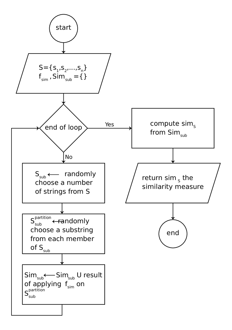
Figure 1: The SCF flowchart. The input is the set of strings, and its output is the amount of similarity among members of $S$. In each iteration, the $SCF$ chooses some substrings from sets and computes their similarity using $f_{sim}$. In the end, the total similarity of $S$ is returned. The similarity value is the measure of classifying $S$.

This framework provides an efficient way to check a set’s similarity dose. It leads to assigning an LCS algorithm to solve the LCS problem more efficiently.

4.2 $S^{2}D$ algorithm for set classification

The previous section proposes the $SCF$ to classify a set of strings based on their similarity. This section proposes Set Similarity Dichotomizer ($S^{2}D$) as an algorithm based on the $SCF$. The $S^{2}D$ algorithm utilizes LCT as $f_{sim}$ to evaluate the similarity of strings. Moreover, it classifies sets into two types “correlated” and “uncorrelated”.

Algorithm 1 shows the steps of the $S^{2}D$ algorithm. $S$ and the parameters, LCT, and end-index ($ei$) are algorithm inputs and represent a set of strings, $f_{sim}$, and the hyper-parameter of the algorithm, respectively. In each iteration, the procedure randomly chooses two strings, $\textbf{s}_{i}$, and $\textbf{s}_{j}$, from $S$, where $1\leq i,j\leq n$, and $i\neq j$. We define $l_{min}$ as the minimum length of $\textbf{s}_{i}$ and $\textbf{s}_{j}$. Then, we separate a part of $\textbf{s}_{i}$ and $\textbf{s}_{j}$ using two start-index (si) and $ei$ parameters. $si\in[1,(l_{min}-ei)]$ is a random number. In fact, $si$ and $ei$ are required to choose a random substring from $\textbf{s}_{i}$ and $\textbf{s}_{j}$. After that, we pass $\textbf{s}_{i}[si:si+ei]$ and $\textbf{s}_{j}[si:si+ei]$ as $S_{sub}$ to the $LCT$ function and obtain the length of the longest common substring, $x$. $S^{2}D$ iterates this process until the convergence. This iteration is necessary to be assured of the $S^{2}D$ result’s reliability. To show the importance of the iteration, we assume the correlated set of $S=\{s_{1}=\texttt{CCGTGCATTT}$, $s_{2}=\texttt{CCGTGCGGCA},s_{3}=\texttt{ACGTGCATT}$, $s_{4}=\texttt{ACGTGCATT}$, $s_{5}=\texttt{CCGTGAATTT}$, $s_{6}=\texttt{CCGTGCATAT}$, $\}$. There is a high correlation among the strings of $S$. Thus, it needs to be labeled as correlated. Nevertheless, if we repeat the $S^{2}D$ in just a single iteration, it is possible to choose the last parts of $s_{1}$ and $s_{2}$ (i.e., CATTT and CGGCA). Then, it labels $S$ as uncorrelated, which is wrong. To avoid this issue, $S^{2}D$ repeats the procedure for several iterations and reduces the probability of such problems. According to our extensive tests, repeating the $S^{2}D$ for $[\frac{n}{2}]$ times guarantees its correctness. Finally, the mean of the $Sim_{sub}$ list is compared to a threshold, and consequently, its type—correlated or uncorrelated—is revealed.

Algorithm 1 $S^{2}D$ algorithm for classifying sets.

$S=\{\textbf{s}_{1},\textbf{s}_{2},\cdots,\textbf{s}_{n}\}$, $LCT(\cdot,\cdot)$, $ei$

$Sim_{sub}=\{\}$

while Not Converged do

     $i,j=random(1,n)$ $\triangleright$ choose a random number between 1 and $n$

     $l_{min}=min(|\textbf{s}_{i}|,|\textbf{s}_{j}|)$

     $si=random(1,\ell_{min}-ei)$

     $x$ = $LCT(\textbf{s}_{i}[si:si+ei],\textbf{s}_{j}[si:si+ei])$

     $Sim_{sub}=Sim_{sub}\cup\{x\}$

end while

$sim_{s}$ = $\mu(Sim_{sub})$

if $sim_{s}>tr$ then

     return “correlated”

else

     return “uncorrelated”

end if

4.3 A novel upper bound hyper-heuristic

As mentioned earlier, while each heuristic has a high performance on some datasets, it has no proper performance for some other datasets. Our observations and experiments show that the upper bound size ($ubs$) is an important property in identifying the goodness of a heuristic function on a set of strings. By introducing the $S^{2}D$ algorithm and having $ubs$, we define a novel hyper-heuristic and name it UB-HH in this paper. It has several advantages. First, it avoids the redundancy of the previous hyper-heuristic, TE-HH. Second, while the TE-HH is designed for just beam search, the UB-HH can be used in any search strategy (e.g., $A^{*}$, greedy search) for solving the LCS problem. Thirdly, it is light and fast in comparison with the TE-HH. Figure 2 illustrates the UB-HH schema. The UB-HH consists of two parts. We refer to the first part as Strings Set Type Recognizer, shown in a green dotted box. It receives the set of strings, and its mission is to determine the set’s type. The second part, surrounded by a red dashed box, contains a set of $LCS$ heuristics. For each given set, UB-HH activates precisely one of the $LCS$ heuristics. The activated heuristic computes the $LCS$ of the given set and returns it as the output of the UB-HH algorithm. Below, we explain the components of the UB-HH in more detail.

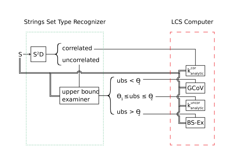
Figure 2: The UB-HH algorithm. It consists of two parts: Strings’ Set Type Recognizer (green dotted box) and LCS Computer (red dashed box). The former contains two modules—the first module ($S^{2}D$) examines the set of strings to identify whether they are correlated. If stamped as uncorrelated, the second module computes the upper bound of the set. Based on the information from the first part, one of the heuristic functions in the second part is activated to compute the LCS.

The Strings Set Type Recognizer part consists of two modules. The first module is the $S^{2}D$ algorithm which determines the class of a given set as correlated and uncorrelated. The correlated strings are directly fed to $k_{analytic}^{cor}$ in the second part of UB-HH to compute its $LCS$. If the given set receives the uncorrelated label, it will be fed into the upper bound examiner module. The upper bound examiner calculates the $ubs$ of the given set using Eq. 6 and divides it by $min(|\textbf{s}_{i}|)$ to map the $ubs$ into the interval $[0,1]$. Then, due to having three base heuristic functions for uncorrelated strings, i.e., BS-Ex, $k_{analytic}^{uncor}$, and GCoV, we define two thresholds, $\theta_{1}$ and $\theta_{2}$, to divide the output of the upper bound examiner into three intervals. Based on the result of ubs, one of them is chosen to find the LCS.

4.4 Complexity analysis of UB-HH

The UB-HH first checks the correlation of the $n$ strings using $S^{2}D$. As algorithm 1 shows, the time complexity of the main loop is O(n). The operations in the loop except for $LCT(\cdot,\cdot)$ are O(1). We use dynamic programming to solve the LCT problem, and its complexity is the multiplication of the length of two input strings [22]. Here, the length of our strings is $ei$. So, the complexity of the LCT procedure is $O(ei^{2})$. Thus, the time complexity of the loop is equal to $O(n\times ei^{2})$. The mean function is out of the loop and its time complexity is O(n). Thus, the total complexity of $S^{2}D$ is $O(n\times ei^{2}+n)$.

The UB-HH runs the upper bound examiner module for the uncorrelated strings. The upper bound examiner computes the $ubs$ of the strings, which is equal to $O(n\times\ell)$ in the worst case. Thus, the complexity of the UB-HH algorithm in the worst case is $O(n\times ei^{2}+n\times\ell+n)$. Because complexity deals with the larger terms, then its whole complexity is either $O(n\times ei^{2})$ or $O(n\times\ell)$—it depends on whether $ei^{2}>\ell$ or vice-versa.

We should note that TE-HH needs to run all heuristics with a smaller beam width ($\beta_{h}$) in advance to find the best LCS heuristic among them. In other words, its time complexity depends on the number and complexity of each base heuristic it uses. We have compared the run time of the UB-HH with the TE-HH in section 5.4.

5 Results

This section provides the results of comparing our proposed methods with the best methods in the LCS literature. To do this, we use three scenarios for comparing methods, low-time, balanced-time-quality, and high-quality. The difference among these scenarios is in their beam widths, which beam width ($\beta$) of low-time, balanced-time-quality, and high-quality are 50, 200, and 600, respectively. This paper proposes a set classifier, $S^{2}D$, and a novel hyper-heuristic UB-HH method. The $S^{2}D$ algorithm classifies sets of strings for the LCS problem. To evaluate our proposed methods, we use six benchmark datasets [23, 24, 13], $ACO$-$Random$, $ACO$-$Rat$, $ACO$-$Virus$, $SARS$-$CoV$-$2$, $BB$, and $ES$. $BB$ and $SARS$-$CoV$-$2$ datasets belong to the correlated class. The ACO-Random, ACO-Rat, ACO-Virus, and $ES$ datasets belong to the uncorrelated class. Each of these datasets contains several sets of strings. Each set has different properties based on the alphabet size ($|\Sigma|$), the length of its corresponding strings ($l$), and the number of strings ($n$). To the best of our knowledge, BS-Ex, BS-GMPSUM, $k_{analytic}^{uncor}$, $k_{analytic}^{cor}$, and GCoV reported the best results on benchmark datasets. So, we compare the UB-HH method with the mentioned methods. In addition to compare the UB-HH with the best methods, we have replaced the base heuristics of TE-HH with the base heuristics used in UB-HH. This replacement yields the comparison of both hyper-heuristics in the same condition. To have a fair comparison, we have re-implemented BS-Ex, BS-GMPSUM, $k_{analytic}^{uncor}$, $k_{analytic}^{cor}$, GCoV, and TE-HH methods in python version $3.8$ programming language. Thus, this section contains the following subsections. Subsection 5.1 reports the way of tuning the algorithms’ parameters in the simulation. Then, we report the performance of the $S^{2}D$ algorithm in section 5.2. Then, to show the performance of the UB-HH algorithm, we compare it with the best heuristics in the LCS literature in section 5.3. subsection 5.4 provides a run time comparison between TE-HH and UB-HH.

5.1 Parameter tuning

To tune parameters, we have generated several new correlated and uncorrelated datasets with different sizes of $|\Sigma|$ in the way that Blum and Blesa [13] generated the BB dataset. In other words, these generated datasets are just for parameter tuning. The mutation (deletion, insertion, change) probability for correlated and uncorrelated is set to 0.1 and 0.9, respectively. For more detail about generating datasets, see [13]. Using grid search [25], we tested different values of ei $=\{10,15,\cdots,\ell\}$, and tr ($1<tr<ei$) for generated datasets. Our extensive experiments revealed that if a set has a common substring with a length greater than $5$, the set in question is correlated. If the length of the common substring becomes lower than $5$, the set is uncorrelated. So, we set the threshold for distinguishing datasets type to $5$. Also, we have observed that a value of ei $\geq 20$ is suitable for the algorithm to work properly. To reduce the algorithm’s run time, we set the value of $ei=20$. When $|\Sigma|=2$, the chance for a common substring with a length greater than $5$ for both types (i.e., correlated and uncorrelated) is high, and all sets are identified as correlated. To address this issue, we reduced the size of ei for sets with $|\Sigma|=2$. To make the long story short, we set ei = 20 and $tr$ = 5 for $|\Sigma|>2$, and ei = 10 and $tr$ = 5 for $|\Sigma|=2$. For tuning the upper bound examiner module parameters (i.e., $\theta_{1}$ and $\theta_{2}$), we tested different values of $\theta$ from a list —$[0.01,0.02,\cdots,1]$— and obtained the best values of $\theta$, which for $\theta_{1}$ is $0.54$ and for $\theta_{2}$ is $0.9$.

5.2 $S^{2}D$ for classifying benchmarks

As introduced in section 4.2, the $S^{2}D$ algorithm classifies any given set of strings for the LCS problem and identifies its label. To the best of our knowledge, $S^{2}D$ is the first case of this type of set classification algorithm in the LCS literature. Thus, there is no other algorithm in this area to compare. Therefore, this section provides the result of applying the $S^{2}D$ algorithm on all mentioned benchmark datasets. Each of the strings’ sets is a sample for $S^{2}D$. This algorithm is applied to all samples provided by datasets, i.e., 751 sets. The $S^{2}D$ classifies instances into two sets of correlated and uncorrelated. Table 2 illustrates the confusion matrix resulting from applying $S^{2}D$ to the benchmark datasets. As the table shows, there are 91 correlated sets, and $S^{2}D$ identified all of them correctly. There are 660 uncorrelated sets, of which the $S^{2}D$ labels 650 correctly and ten wrongly. So, the $S^{2}D$’s accuracy is $98\%$. The wrong labels belong to those sets with an alphabet length equal to 2. The problem with $|\Sigma|=2$ is that existing of the exact binary substrings has a high probability.

Table 2: The confusion matrix of applying $S^{2}D$ on all sets available in $ACO$-$Rat$, $ACO$-$Virus$, $ACO$-$Random$, $ES$, $BB$, and $SARS$-$CoV$-$2$ datasets.

	Correlated	Uncorrelated
Correlated	91	10
Uncorrelated	0	650

5.3 Comparison of UB-HH with best methods

Here, we compare the performance of the UB-HH algorithm with the best methods in three mentioned scenarios over six mentioned benchmarks. Subsection 5.3.1 provides the result of balanced-time-quality, or $\beta=200$. In addition to the balanced-time-quality scenario ($\beta=200$), we provide two more scenarios of low-time ($\beta=50$) and high-quality ($\beta=600$) in the following subsections to fairly compare our proposal with existing methods in the literature. We call the $\beta=200$ as balanced-time-quality due to having both balances in time and quality simultaneously compared to the low-time and high-quality. Therefore, subsection 5.3.2 reports the low-time scenario, or $\beta=50$. Subsection 5.3.3 contains the result of the high-quality scenario, or $\beta=600$.

5.3.1 balanced-time-quality comparison of best methods

This subsection provides balanced-time-quality scenario, which is a new setting in which time and quality are in a balanced mode. Here, we compare UB-HH with the best methods and TE-HH. The TE-HH has two versions. The first one is the original base heuristics (i.e., h-prob and h-power). Instead of the original paper setting, we have replaced the base heuristics of TE-HH with the UB-HH base heuristics (i.e., BS-Ex, $k_{analytic}^{cor}$, $k_{analytic}^{uncor}$, and GCoV) in this paper. This update enables us to compare hyper-heuristics in a fair condition. TE-HH, in addition to the conventional beam width ($\beta$), intrinsically needs a parameter called trial beam width ($\beta_{h}$) to find the best base heuristic; we use the value noted in the original paper [20] for $\beta_{h}$, which is 50. Tables 3– 8 show the comparison among the best methods, TE-HH, and UB-HH. The UB-HH achieves the best results in five out of six benchmarks (i.e., ACO-Random, ACO-Rat, SARS-CoV-2, BB, and ES). Concerning LCS average length for each benchmark, UB-HH is the winner in ACO-Random, ACO-Rat, SARS-CoV-2, and ES benchmarks. For the ACO-Virus benchmark, BS-GMPSUM is better than other methods in both LCS average length and number of best solutions. In the BB benchmark, TE-HH obtains a longer average LCS length than others. As the results show, the UB-HH generally outperforms other methods in the case of $\beta=200$.

Table 3: Comparison of best methods, TE-HH, and UB-HH over ACO-Random benchmark in balanced-time-quality scenario.

$|\Sigma|$	$\ell$	n	BS-GMPSUM	$k_{analytic}^{cor}$	$k_{analytic}^{uncor}$	BS-Ex	GCoV	TE-HH	UB-HH
4	600	10	218	215	220	220	217	217	220
4	600	15	202	201	202	203	199	203	202
4	600	20	191	189	192	191	187	191	192
4	600	25	188	186	187	186	183	186	187
4	600	40	173	172	175	174	170	174	175
4	600	60	165	164	167	167	161	167	167
4	600	80	161	160	162	161	157	162	162
4	600	100	159	157	159	159	154	159	159
4	600	150	151	152	153	153	149	153	153
4	600	200	149	149	151	150	147	151	151
20	600	10	61	61	62	62	61	62	62
20	600	15	51	50	51	51	51	51	51
20	600	20	47	46	47	47	47	47	47
20	600	25	44	44	44	44	44	44	44
20	600	40	38	38	39	38	38	38	39
20	600	60	35	34	35	35	35	35	35
20	600	80	33	32	33	33	33	33	33
20	600	100	32	31	32	32	32	32	32
20	600	150	29	29	29	29	29	29	29
20	600	200	28	28	28	27	28	28	28
Average			107.75	106.9	108.4	108.1	106.05	108.1	108.4

Table 4: Comparison of best methods, TE-HH, and UB-HH over ACO-Rat benchmark in balanced-time-quality scenario.

$|\Sigma|$	$\ell$	n	BS-GMPSUM	$k_{analytic}^{cor}$	$k_{analytic}^{uncor}$	BS-Ex	GCoV	TE-HH	UB-HH
4	600	10	198	197	202	201	198	201	202
4	600	15	184	181	184	183	182	183	184
4	600	20	173	165	172	171	169	172	169
4	600	25	169	164	169	171	167	169	169
4	600	40	155	143	151	148	155	155	155
4	600	60	152	150	152	152	148	152	152
4	600	80	141	136	139	140	141	141	141
4	600	100	138	130	135	136	136	136	136
4	600	150	124	123	129	128	129	129	129
4	600	200	121	119	122	124	123	123	123
20	600	10	70	68	70	70	70	70	70
20	600	15	62	61	62	62	62	62	62
20	600	20	54	53	54	54	54	54	54
20	600	25	51	50	51	51	52	51	52
20	600	40	48	49	49	48	49	49	49
20	600	60	46	46	46	46	46	46	46
20	600	80	43	43	43	43	43	43	43
20	600	100	40	38	39	39	40	39	40
20	600	150	37	36	37	37	37	37	37
20	600	200	34	32	34	34	35	34	35
Average			102	99.2	102	101.9	101.8	102.3	102.4

Table 5: Comparison of best methods, TE-HH, and UB-HH over ACO-Virus benchmark in balanced-time-quality scenario.

$|\Sigma|$	$\ell$	n	BS-GMPSUM	$k_{analytic}^{cor}$	$k_{analytic}^{uncor}$	BS-Ex	GCoV	TE-HH	UB-HH
4	600	10	225	223	223	223	218	223	223
4	600	15	203	203	203	202	204	202	203
4	600	20	191	187	190	189	189	189	190
4	600	25	194	192	193	193	190	193	193
4	600	40	170	167	170	169	168	170	170
4	600	60	167	164	166	166	162	166	166
4	600	80	161	159	161	162	156	161	161
4	600	100	158	155	156	157	154	157	156
4	600	150	152	155	156	155	152	156	156
4	600	200	149	153	155	153	149	153	155
20	600	10	74	74	74	74	75	75	75
20	600	15	62	62	63	64	62	63	62
20	600	20	59	58	59	59	59	59	59
20	600	25	55	54	55	54	55	55	55
20	600	40	51	49	50	49	49	50	49
20	600	60	48	47	48	48	47	47	47
20	600	80	46	46	46	46	45	46	45
20	600	100	44	44	44	43	44	43	44
20	600	150	45	45	45	45	45	45	45
20	600	200	44	44	43	44	43	43	43
Average			114.9	114.05	115	114.75	113.3	114.8	114.85

Table 6: Comparison of best methods, TE-HH, and UB-HH over SARS-CoV-2 benchmark in balanced-time-quality scenario.

$|\Sigma|$	$\ell$	n	BS-GMPSUM	$k_{analytic}^{cor}$	$k_{analytic}^{uncor}$	BS-Ex	GCoV	TE-HH	UB-HH
4	400	10	189	198	179	182	172	179	198
4	400	20	193	191	195	189	176	191	191
4	400	30	178	175	174	173	156	175	175
4	400	40	164	168	154	150	146	168	168
4	400	50	157	160	156	145	141	160	160
4	400	60	153	153	146	139	139	153	153
4	400	70	148	142	140	137	136	140	142
4	400	80	151	150	147	140	140	150	150
4	400	90	158	163	152	150	145	163	163
4	400	100	144	148	140	139	132	148	148
4	400	110	141	143	142	143	133	143	143
Average			161.45	162.81	156.81	153.4	146.9	160.9	162.81

Table 7: Comparison of best methods, TE-HH, and UB-HH over BB benchmark in balanced-time-quality scenario.

$|\Sigma|$	$\ell$	n	BS-GMPSUM	$k_{analytic}^{cor}$	$k_{analytic}^{uncor}$	BS-Ex	GCoV	TE-HH	UB-HH
2	1000	10	629	635.7	594.1	604.8	614.1	631.5	635.7
2	1000	100	556	559.4	540.3	531.3	543.1	559.4	559.4
4	1000	10	467.5	464.3	426.9	424.4	452.4	463.4	464.3
4	1000	100	364.5	365.6	341.8	324.7	365.3	366.6	365.6
8	1000	10	343.4	359.6	307.2	289.9	359.5	368.3	359.6
8	1000	100	244.1	242.1	217	201.5	244.3	242.5	242.1
24	1000	10	263	274.1	226.7	220.6	277.1	296.7	274.1
24	1000	100	128.9	130.8	112.4	102.2	123	127.5	130.8
Average			374.63	378.95	345.8	337.42	372.35	381.98	378.95

Table 8: Comparison of best methods, TE-HH, and UB-HH over ES benchmark in balanced-time-quality scenario.

$|\Sigma|$	$\ell$	n	BS-GMPSUM	$k_{analytic}^{cor}$	$k_{analytic}^{uncor}$	BS-Ex	GCoV	TE-HH	UB-HH
2	1000	10	603.72	600.8	584.84	609.96	527.28	609.96	609.96
2	1000	50	353.98	532.66	531.62	537.02	510.8	537.02	536.9
2	1000	100	518.12	515.28	519	518.96	500.2	518.84	518.96
10	1000	10	197.44	195.32	198.88	199.16	190.13	198.86	198.88
10	1000	50	135.34	134.38	135.68	135.66	127.53	135.48	135.68
10	1000	100	122.74	121.72	122.82	122.7	116.35	122.62	122.82
25	2500	10	229.04	226.4	229.9	226.06	214.06	229.8	229.9
25	2500	50	138.61	136.98	138.74	138.7	128.92	138.66	138.74
25	2500	100	122.21	121.04	122.3	122.38	113.33	122.22	122.3
100	5000	10	138.98	137.36	139.08	138.94	134.81	138.98	139.08
100	5000	50	70.9	69.84	71	70.98	66.3	70.98	71
100	5000	100	59.93	59.2	60.06	59.98	56.74	60.04	60.06
Average			239.41	237.58	237.82	240.04	227.62	240.028	240.35

5.3.2 low-time comparison of best methods

We set the $\beta$ for all methods to $50$ in the second scenario — low-time scenario. Tables 9– 14 show the detailed comparison of UB-HH with the best methods in the low-time scenario. The UB-HH obtains the highest LCS average length and number of best solutions in four of six benchmarks, i.e., ACO-Random, ACO-Rat, BB, and ES. In the case of the ACO-Virus dataset, $k_{analytic}^{uncor}$ could obtain the best average rank and the highest number of best solutions. For the SARS-CoV-2 dataset, BS-GMPSUM is the winner in both LCS average length and number of best solutions. To sum up, the lowest average rank belongs to UB-HH in general in the case of $\beta=50$.

Table 9: Comparison of best methods and UB-HH over ACO-Random benchmark in low-time scenario.

$|\Sigma|$	$\ell$	n	BS-GMPSUM	$k_{analytic}^{cor}$	$k_{analytic}^{uncor}$	BS-Ex	GCoV	UB-HH
4	600	10	211	214	215	215	217	215
4	600	15	196	197	201	201	196	201
4	600	20	189	187	191	191	187	191
4	600	25	184	182	184	186	181	184
4	600	40	171	170	173	173	168	173
4	600	60	164	163	166	166	159	166
4	600	80	159	158	161	161	154	161
4	600	100	157	156	158	158	152	158
4	600	150	150	151	152	152	148	152
4	600	200	149	148	151	150	147	151
20	600	10	59	58	61	61	61	61
20	600	15	50	50	51	50	50	51
20	600	20	46	43	46	47	46	46
20	600	25	43	43	43	43	43	43
20	600	40	37	38	38	38	38	38
20	600	60	34	34	34	34	34	34
20	600	80	32	32	33	32	32	33
20	600	100	31	31	31	31	31	31
20	600	150	29	29	29	29	29	29
20	600	200	28	28	28	27	28	28
Average			105.95	105.6	107.3	107.25	105.05	107.3

Table 10: Comparison of best methods and UB-HH over ACO-Rat benchmark in low-time scenario.

$|\Sigma|$	$\ell$	n	BS-GMPSUM	$k_{analytic}^{cor}$	$k_{analytic}^{uncor}$	BS-Ex	GCoV	UB-HH
4	600	10	197	192	198	198	196	198
4	600	15	179	179	180	182	180	180
4	600	20	168	165	170	169	169	169
4	600	25	163	161	167	166	166	167
4	600	40	144	137	144	143	150	150
4	600	60	148	147	152	150	148	152
4	600	80	136	136	139	138	140	140
4	600	100	128	129	134	136	134	134
4	600	150	123	121	129	127	127	127
4	600	200	120	119	118	121	124	124
20	600	10	68	68	69	70	69	69
20	600	15	62	59	62	62	60	60
20	600	20	53	52	52	52	52	52
20	600	25	51	50	50	51	51	51
20	600	40	48	48	47	47	49	49
20	600	60	46	46	46	45	47	47
20	600	80	43	42	42	41	43	43
20	600	100	38	37	38	38	38	38
20	600	150	36	35	37	36	37	37
20	600	200	33	32	33	34	33	33
Average			99.2	97.75	100.35	100.3	100.65	101

Table 11: Comparison of best methods and UB-HH over ACO-Virus benchmark in low-time scenario.

$|\Sigma|$	$\ell$	n	BS-GMPSUM	$k_{analytic}^{cor}$	$k_{analytic}^{uncor}$	BS-Ex	GCoV	UB-HH
4	600	10	221	220	223	223	218	223
4	600	15	198	199	201	201	199	201
4	600	20	187	186	187	189	189	187
4	600	25	191	191	190	190	188	190
4	600	40	167	165	168	167	165	168
4	600	60	162	162	163	162	161	163
4	600	80	157	156	157	158	155	157
4	600	100	153	152	155	156	154	155
4	600	150	154	155	155	154	150	155
4	600	200	153	153	153	152	149	153
20	600	10	74	72	73	73	75	75
20	600	15	61	61	63	63	60	60
20	600	20	58	58	59	59	59	59
20	600	25	55	53	55	54	55	55
20	600	40	49	49	50	49	49	49
20	600	60	46	46	46	46	46	46
20	600	80	45	44	46	45	45	45
20	600	100	44	44	44	44	43	43
20	600	150	45	45	45	45	44	44
20	600	200	43	43	43	42	43	43
Average			113.15	112.7	113.8	113.6	112.35	113.55

Table 12: Comparison of best methods and UB-HH over SARS-CoV-2 benchmark in low-time scenario.

$|\Sigma|$	$\ell$	n	BS-GMPSUM	$k_{analytic}^{cor}$	$k_{analytic}^{uncor}$	BS-Ex	GCoV	UB-HH
4	400	10	189	192	195	186	168	192
4	400	20	195	190	186	183	175	190
4	400	30	190	176	167	160	156	176
4	400	40	154	157	151	144	146	157
4	400	50	153	152	151	148	143	152
4	400	60	147	149	143	142	136	149
4	400	70	139	139	143	134	133	139
4	400	80	148	146	146	139	135	146
4	400	90	155	155	152	152	137	155
4	400	100	141	140	139	139	129	140
4	400	110	144	143	140	135	127	143
Average			159.54	158.09	155.72	151.09	144.09	158.09

Table 13: Comparison of best methods and UB-HH over BB benchmark in low-time scenario.

$|\Sigma|$	$\ell$	n	BS-GMPSUM	$k_{analytic}^{cor}$	$k_{analytic}^{uncor}$	BS-Ex	GCoV	UB-HH
2	1000	10	627.6	625.6	587.1	607.6	613.1	625.6
2	1000	100	551.4	553.7	532.5	525.2	539.3	553.7
4	1000	10	462.3	454.2	420.2	413.3	451.2	454.2
4	1000	100	359	357.7	338.1	319	359.7	357.7
8	1000	10	361.5	366.3	306.4	294.2	367.2	366.3
8	1000	100	233.6	231.5	210.8	195.6	240.5	231.5
24	1000	10	262.8	274.6	240.1	204.3	265.7	274.6
24	1000	100	121.3	125	103.2	96.9	123.6	125
Average			372.43	373.57	342.3	332.01	370.03	373.57

Table 14: Comparison of best methods and UB-HH over ES benchmark in low-time scenario.

$|\Sigma|$	$\ell$	n	BS-GMPSUM	$k_{analytic}^{cor}$	$k_{analytic}^{uncor}$	BS-Ex	GCoV	UB-HH
2	1000	10	600.92	597.98	582.56	607.22	584.2	607.22
2	1000	50	533.6	530.46	529.6	535.04	513	535.04
2	1000	100	516.16	513.6	517.52	517.34	502.6	517.34
10	1000	10	195.18	194.16	196.84	197.18	193.1	196.84
10	1000	50	134.28	133.04	134.62	134.48	129	134.62
10	1000	100	121.94	120.86	122.04	121.94	117.8	122.04
25	2500	10	225.6	224.22	227.76	221.2	220.4	227.76
25	2500	50	137.32	135.82	137.64	137.82	130.4	137.64
25	2500	100	121.6	120.2	121.6	121.74	114.7	121.6
100	5000	10	135.64	135.34	137.72	135.64	132.1	137.72
100	5000	50	70.21	69.14	70.3	70.38	67.8	70.3
100	5000	100	59.33	58.76	59.6	59.6	58.1	59.6
Average			237.64	236.13	236.48	238.29	230.27	238.97

5.3.3 high-quality comparison of best methods

In the third scenario, we compare the UB-HH algorithm with the best methods in the high-quality setting, where it is $\beta=600$. Tables 15– 20 show that the UB-HH obtains a higher number of best solutions in four out of six benchmarks (i.e., ACO-Rat, SARS-CoV-2, BB, and ES) and the best LCS average length in ACO-Rat, BB, and ES benchmarks. BS-Ex obtains a better LCS average length and more best solutions concerning the ACO-Random benchmark. For ACO-Virus, BS-GMPSUM is better than other methods in both LCS average length and number of best solutions. However, concerning the lowest average rank, UB-HH is better than all methods overall.

Table 15: Comparison of best methods and UB-HH over ACO-Random benchmark in high-quality scenario.

$|\Sigma|$	$\ell$	n	BS-GMPSUM	$k_{analytic}^{cor}$	$k_{analytic}^{uncor}$	BS-Ex	GCoV	UB-HH
4	600	10	218	215	218	219	216	218
4	600	15	204	203	204	204	201	204
4	600	20	192	191	193	193	190	193
4	600	25	187	186	187	187	184	187
4	600	40	174	172	175	175	170	175
4	600	60	167	166	168	168	162	168
4	600	80	162	160	162	163	159	162
4	600	100	159	158	159	159	155	159
4	600	150	152	152	153	153	149	153
4	600	200	150	149	151	151	148	151
20	600	10	62	61	62	62	62	62
20	600	15	52	51	51	51	51	51
20	600	20	47	47	47	47	47	47
20	600	25	44	44	44	44	44	44
20	600	40	39	38	39	39	38	39
20	600	60	35	34	35	35	35	35
20	600	80	33	33	33	33	33	33
20	600	100	32	31	32	32	31	32
20	600	150	29	29	29	29	29	29
20	600	200	28	28	28	27	28	28
Average			108.3	107.4	108.5	108.55	106.6	108.5

Table 16: Comparison of best methods and UB-HH over ACO-Rat benchmark in high-quality scenario.

$|\Sigma|$	$\ell$	n	BS-GMPSUM	$k_{analytic}^{cor}$	$k_{analytic}^{uncor}$	BS-Ex	GCoV	UB-HH
4	600	10	200	198	204	204	202	204
4	600	15	183	183	185	185	184	185
4	600	20	173	167	173	172	171	171
4	600	25	169	165	170	170	168	170
4	600	40	155	145	148	152	153	153
4	600	60	153	149	152	152	149	152
4	600	80	141	137	142	142	140	140
4	600	100	137	134	135	137	137	137
4	600	150	125	124	128	129	129	129
4	600	200	119	119	123	124	124	124
20	600	10	70	70	70	70	70	70
20	600	15	62	62	62	63	62	62
20	600	20	54	53	54	54	54	54
20	600	25	51	50	51	51	52	52
20	600	40	48	49	49	49	50	50
20	600	60	47	46	47	46	48	48
20	600	80	43	44	43	43	44	44
20	600	100	40	39	39	40	40	40
20	600	150	38	36	38	37	38	38
20	600	200	35	33	35	34	35	35
Average			102.15	100.15	102.4	102.7	102.5	102.9

Table 17: Comparison of best methods and UB-HH over ACO-Virus benchmark in high-quality scenario.

$|\Sigma|$	$\ell$	n	BS-GMPSUM	$k_{analytic}^{cor}$	$k_{analytic}^{uncor}$	BS-Ex	GCoV	UB-HH
4	600	10	225	224	223	223	222	223
4	600	15	203	201	204	205	202	204
4	600	20	191	187	190	192	191	190
4	600	25	195	193	194	194	193	194
4	600	40	171	168	171	170	168	171
4	600	60	167	164	166	166	165	166
4	600	80	162	159	160	163	158	160
4	600	100	160	158	159	158	155	159
4	600	150	156	156	157	156	152	157
4	600	200	150	154	155	154	151	155
20	600	10	76	74	75	76	75	75
20	600	15	63	63	64	64	63	63
20	600	20	59	59	59	59	60	60
20	600	25	55	54	55	54	55	55
20	600	40	51	49	50	50	51	51
20	600	60	48	47	48	48	48	48
20	600	80	46	46	46	46	46	46
20	600	100	45	44	45	44	44	44
20	600	150	45	45	45	45	45	45
20	600	200	44	44	43	43	44	44
Average			115.6	114.45	115.45	115.5	114.4	115.5

Table 18: Comparison of best methods and UB-HH over SARS-CoV-2 benchmark in high-quality scenario.

$|\Sigma|$	$\ell$	n	BS-GMPSUM	$k_{analytic}^{cor}$	$k_{analytic}^{uncor}$	BS-Ex	GCoV	UB-HH
4	400	10	196	198	195	201	168	198
4	400	20	224	224	187	189	176	224
4	400	30	183	173	187	174	166	173
4	400	40	164	169	156	153	146	169
4	400	50	161	160	156	156	146	160
4	400	60	155	156	153	150	143	156
4	400	70	149	143	143	139	141	143
4	400	80	158	153	150	146	138	153
4	400	90	163	161	154	150	139	161
4	400	100	144	146	143	142	136	146
4	400	110	149	150	145	144	134	150
Average			167.81	166.63	160.81	158.54	148.45	166.63

Table 19: Comparison of best methods and UB-HH over BB benchmark in high-quality scenario.

$|\Sigma|$	$\ell$	n	BS-GMPSUM	$k_{analytic}^{cor}$	$k_{analytic}^{uncor}$	BS-Ex	GCoV	UB-HH
2	1000	10	632.8	634.9	587.4	614.6	620.9	634.9
2	1000	100	560.9	562	541.8	536.3	544.7	562
4	1000	10	468.2	453	421	419.2	459.8	453
4	1000	100	366.8	372.3	345.9	328.1	366.4	372.3
8	1000	10	353.9	341.4	317.6	303.6	363.1	341.4
8	1000	100	246.1	247.9	222.6	209.4	242.8	247.9
24	1000	10	265.1	281.8	233	225.6	272.5	281.8
24	1000	100	130.7	134.1	114.7	109.5	127.8	134.1
Average			378.06	378.42	348	343.28	374.75	378.42

Table 20: Comparison of best methods and UB-HH over ES benchmark in high-quality scenario.

$|\Sigma|$	$\ell$	n	BS-GMPSUM	$k_{analytic}^{cor}$	$k_{analytic}^{uncor}$	BS-Ex	GCoV	UB-HH
2	1000	10	605.94	603	585.94	611.48	593.52	611.48
2	1000	50	537.08	533.94	532.6	538.22	517.7	538.22
2	1000	100	519.28	516.26	519.92	519.84	503.62	519.84
10	1000	10	198.72	197.42	200.6	200.68	199.1	200.6
10	1000	50	136.19	134.96	136.22	136.14	132.1	136.22
10	1000	100	122.76	122.18	123.28	123.22	119.6	123.28
25	2500	10	229.9	228.76	231.92	228.5	221.2	231.92
25	2500	50	139.23	137.66	139.38	139.34	133.4	139.38
25	2500	100	122.65	121.44	122.78	122.74	119.71	122.78
100	5000	10	140.75	139.45	140.78	141.14	137.1	140.78
100	5000	50	71.27	70.1	71.28	71.32	67.5	71.28
100	5000	100	60.08	59.84	60.12	60.16	56.94	60.12
Average			240.32	238.75	238.73	241.06	233.45	241.32

5.4 Time comparison

Here, we compare the run time aspect of TE-HH and UB-HH to choose the suitable heuristic among the base heuristics. TE-HH needs to run all its base heuristics with $\beta_{h}$. So, by having four base heuristics, TE-HH run time is the summation of the running time of BS-Ex, $k_{analytic}^{cor}$, $k_{analytic}^{uncor}$, and GCoV with $\beta_{h}$. In contrast, UB-HH does not need to run base heuristics, and it instantly finds the suitable base heuristic based on strings’ internal properties (less than one second). Among six datasets, Fig. 3 shows the run time of TE-HH and UB-HH on the ACO-Random dataset. As the figure shows, UB-HH can instantly specify the suitable heuristic, but TE-HH run time depends on the run time of all heuristics and is very high compared to UB-HH. The same pattern happens for the other five benchmarks i.e., ACO-Rat, ACO-Virus, SARS-CoV-2, BB, and ES.

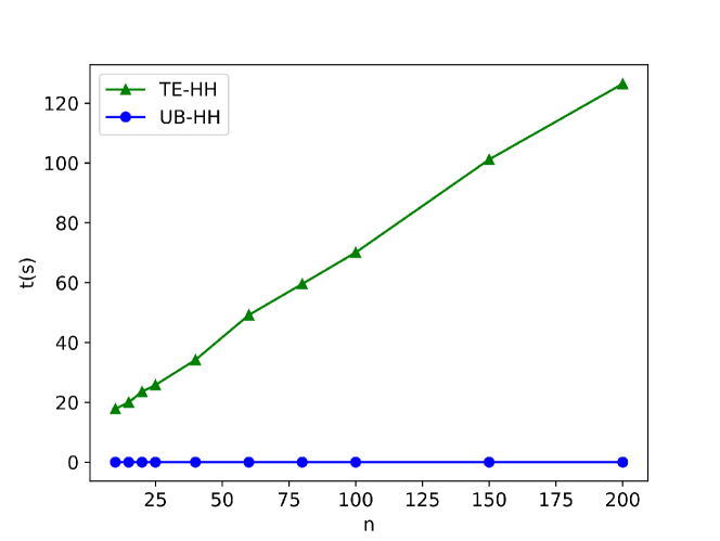
Figure 3: Comparison of the run time of TE-HH and UB-HH on ACO-Random dataset with $|\Sigma|=4$. The same pattern happens for other datasets.

6 Statistical analysis

In this section, we perform the statistical significance tests for all running scenarios: low-time, high-quality, and balanced-time-quality. For this purpose, we use the Friedman [26] test with the $5\%$ error level. Also, the Nemenyi post-hoc [27] test is employed to check the pairwise significance of algorithms.
Fig. 4 shows the critical difference plot for all methods on all benchmarks on the balanced-time-quality scenario. UB-HH is significantly better than all methods except TE-HH. In comparing UB-HH and TE-HH, these two algorithms perform equally on all benchmark datasets. However, in the case of uncorrelated benchmarks (i.e., ACO-Random, ACO-Rat, ACO-Virus, ES), the UB-HH is significantly better than TE-HH.

((a)) GCoV and UB-HH

((b)) BS-Ex and UB-HH

((c)) $k_{analytic}^{cor}$ and UB-HH

((d)) BS-GMPSUM and UB-HH

((e)) $k_{analytic}^{uncor}$ and UB-HH

((f)) TE-HH and UB-HH

Figure 4: Critical difference plot in balanced-time-quality setting for all considered benchmarks

Fig. 5 shows the critical difference plot for all methods on all benchmarks in the low-time scenario. UB-HH is significantly better than other methods except for $k_{analytic}^{uncor}$, which they perform equally.

((a)) GCoV and UB-HH

((b)) BS-Ex and UB-HH

((c)) $k_{analytic}^{cor}$ and UB-HH

((d)) BS-GMPSUM and UB-HH

((e)) $k_{analytic}^{uncor}$ and UB-HH

Figure 5: Critical difference plot in low-time setting for all considered benchmarks

Fig. 6 shows the critical difference plot for all methods on all benchmarks in the high-time scenario. UB-HH is significantly better than all methods.

((a)) GCoV and UB-HH

((b)) BS-Ex and UB-HH

((c)) $k_{analytic}^{cor}$ and UB-HH

((d)) BS-GMPSUM and UB-HH

((e)) $k_{analytic}^{uncor}$ and UB-HH

Figure 6: Critical difference plot in high-quality setting for all considered benchmarks

7 Conclusion

In this work, we have proposed, the SCF framework and $S^{2}D$ algorithm to classify a given set of strings for the first time. Set classification is an initial stage to choose the best matching LCS algorithm for a given set of strings. The $S^{2}D$ algorithm can classify all benchmarks in the LCS literature with $98\%$ accuracy. By employing the $S^{2}D$ algorithm and the upper bound value, we have introduced the hyper-heuristic UB-HH to identify the best heuristic for any set of strings. Unlike TE-HH, the UB-HH is very fast and independent of the “search strategy”. The results show that our proposed hyper-heuristic (UB-HH) outperforms TE-HH, even with the same base heuristics in both solution quality and run time factors. In future work, it is possible to use other properties of strings, e.g., information measures or complexity standards, instead of upper bound to recognize the relevant heuristic. Furthermore, designing high-quality heuristics for correlated strings enriches the available methods of correlated datasets.

References

- [1] T. F. Smith, M. S. Waterman, et al., Identification of common molecular subsequences, Journal of molecular biology 147 (1) (1981) 195–197.
- [2] T. Jiang, G. Lin, B. Ma, K. Zhang, A general edit distance between rna structures, Journal of computational biology 9 (2) (2002) 371–388.
- [3] R. Shikder, P. Thulasiraman, P. Irani, P. Hu, An openmp-based tool for finding longest common subsequence in bioinformatics, BMC research notes 12 (1) (2019) 1–6.
- [4] S.-Y. Lu, K. S. Fu, A sentence-to-sentence clustering procedure for pattern analysis, IEEE Transactions on Systems, Man, and Cybernetics 8 (5) (1978) 381–389.
- [5] J. Huang, Z. Fang, H. Kasai, Lcs graph kernel based on wasserstein distance in longest common subsequence metric space, Signal Processing 189 (2021) 108281.
- [6] J. B. Kruskal, An overview of sequence comparison: Time warps, string edits, and macromolecules, SIAM review 25 (2) (1983) 201–237.
- [7] A. Banerjee, J. Ghosh, Clickstream clustering using weighted longest common subsequences, in: Proceedings of the web mining workshop at the 1st SIAM conference on data mining, Vol. 143, Citeseer, 2001, p. 144.
- [8] H. Dong, J. Man, L. Jia, X. Wang, Y. Qin, K. Liu, Traffic speed estimation using mobile phone location data based on longest common subsequence, in: 2018 21st International Conference on Intelligent Transportation Systems (ITSC), IEEE, 2018, pp. 2819–2824.
- [9] J. Ding, J. Fang, Z. Zhang, P. Zhao, J. Xu, L. Zhao, Real-time trajectory similarity processing using longest common subsequence, in: 2019 IEEE 21st International Conference on High Performance Computing and Communications; IEEE 17th International Conference on Smart City; IEEE 5th International Conference on Data Science and Systems (HPCC/SmartCity/DSS), 2019, pp. 1398–1405. doi:10.1109/HPCC/SmartCity/DSS.2019.00194.
- [10] D. Maier, The complexity of some problems on subsequences and supersequences, Journal of the ACM (JACM) 25 (2) (1978) 322–336.
- [11] M. Djukanovic, G. R. Raidl, C. Blum, A beam search for the longest common subsequence problem guided by a novel approximate expected length calculation, in: International Conference on Machine Learning, Optimization, and Data Science, Springer, 2019, pp. 154–167.
- [12] A. Abdi, M. Hooshmand, Longest common subsequence: Tabular vs. closed-form equation computation of subsequence probability, arXiv preprint arXiv:2206.11726.
- [13] C. Blum, M. J. Blesa, Probabilistic beam search for the longest common subsequence problem, in: International Workshop on Engineering Stochastic Local Search Algorithms, Springer, 2007, pp. 150–161.
- [14] P. Norvig, Paradigms of artificial intelligence programming: case studies in Common LISP, Morgan Kaufmann, 1992.
- [15] C. Blum, M. J. Blesa, M. López-Ibáñez, Beam search for the longest common subsequence problem, Computers & Operations Research 36 (12) (2009) 3178–3186.
- [16] S. R. Mousavi, F. Tabataba, An improved algorithm for the longest common subsequence problem, Computers & Operations Research 39 (3) (2012) 512–520.
-
[17]
A. Aho, M. Lam, R. Sethi, J. Ullman,
Compilers: Principles,
Techniques, & Tools, Pearson/Addison Wesley, 2007.
URL https://books.google.nl/books?id=dIU_AQAAIAAJ -
[18]
B. Nikolic, A. Kartelj, M. Djukanovic, M. Grbic, C. Blum, G. Raidl,
Solving the longest common
subsequence problem concerning non-uniform distributions of letters in input
strings, Mathematics 9 (13).
doi:10.3390/math9131515.
URL https://www.mdpi.com/2227-7390/9/13/1515 - [19] E. Burke, G. Kendall, J. Newall, E. Hart, P. Ross, S. Schulenburg, Hyper-heuristics: An emerging direction in modern search technology, in: Handbook of metaheuristics, Springer, 2003, pp. 457–474.
- [20] F. S. Tabataba, S. R. Mousavi, A hyper-heuristic for the longest common subsequence problem, Computational biology and chemistry 36 (2012) 42–54.
- [21] B. Everitt, The cambridge dictionary of statistics cambridge university press, Cambridge, UK Google Scholar.
- [22] D. Gusfield, Algorithms on stings, trees, and sequences: Computer science and computational biology, Acm Sigact News 28 (4) (1997) 41–60.
- [23] S. J. Shyu, C.-Y. Tsai, Finding the longest common subsequence for multiple biological sequences by ant colony optimization, Computers & Operations Research 36 (1) (2009) 73–91.
- [24] T. Easton, A. Singireddy, A large neighborhood search heuristic for the longest common subsequence problem, J. Heuristics 14 (2008) 271–283. doi:10.1007/s10732-007-9038-y.
- [25] H. A. Fayed, A. F. Atiya, Speed up grid-search for parameter selection of support vector machines, Applied Soft Computing 80 (2019) 202–210.
- [26] M. Friedman, A comparison of alternative tests of significance for the problem of m rankings, The Annals of Mathematical Statistics 11 (1) (1940) 86–92.
- [27] J. Demšar, Statistical comparisons of classifiers over multiple data sets, The Journal of Machine learning research 7 (2006) 1–30.