Image Inpainting via Iteratively Decoupled Probabilistic Modeling

Abstract

Generative adversarial networks (GANs) have made great success in image inpainting yet still have difficulties tackling large missing regions. In contrast, iterative probabilistic algorithms, such as autoregressive and denoising diffusion models, have to be deployed with massive computing resources for decent effect. To achieve high-quality results with low computational cost, we present a novel pixel spread model (PSM) that iteratively employs decoupled probabilistic modeling, combining the optimization efficiency of GANs with the prediction tractability of probabilistic models. As a result, our model selectively spreads informative pixels throughout the image in a few iterations, largely enhancing the completion quality and efficiency. On multiple benchmarks, we achieve new state-of-the-art performance. Code is released at https://github.com/fenglinglwb/PSM.

Figure 1: Our model supports photo-realistic large-hole inpainting for various scenarios. The first example for object removal is a high-resolution image captured in the wild, while other inpainting examples ($512\times 512$) come from Places2 [82] and CelebA-HQ [23] datasets.

1 Introduction

Image inpainting, a fundamental computer vision task, aims to fill the missing regions in an image with visually pleasing and semantically appropriate content. It has been extensively employed in graphics and imaging applications, such as photo restoration [60, 61], image editing [3, 21], compositing [32], re-targeting [8], and object removal [10]. This task, especially filling large holes, is more ill-posed than other restoration problems, necessitating models of stronger generation abilities.

In past years, generative adversarial networks (GANs) have made great processes in image inpainting [43, 69, 71, 37, 62, 34]. By implicitly modeling a target distribution through a min-max game, GANs-based methods significantly outperform traditional exemplar-based techniques [16, 55, 10, 9] in terms of visual quality. However, the one-shot generation of GANs sometimes lead to unstable training [51, 14, 28] and makes it challenging to learn a complex distribution, particularly when inpainting large holes in high-resolution images.

Conversely, autoregressive models [57, 58, 42] and denoising diffusion models [53, 19, 11] recently demonstrated remarkable power in content generation [44, 49, 73, 52]. These models utilize tractable probabilistic modeling techniques to iteratively refine the image based on prior estimations, resulting in more stable training and improved coverage. However, it is widely known that autoregressive models process images pixel by pixel, which makes it cumbersome to handle high-resolution data. On the other hand, denoising diffusion models typically require thousands of iterations to achieve accurate estimations. Thus, using these methods directly in image inpainting incurs respective drawbacks – strategies for high-quality large-hole high-resolution image inpainting still fall short.

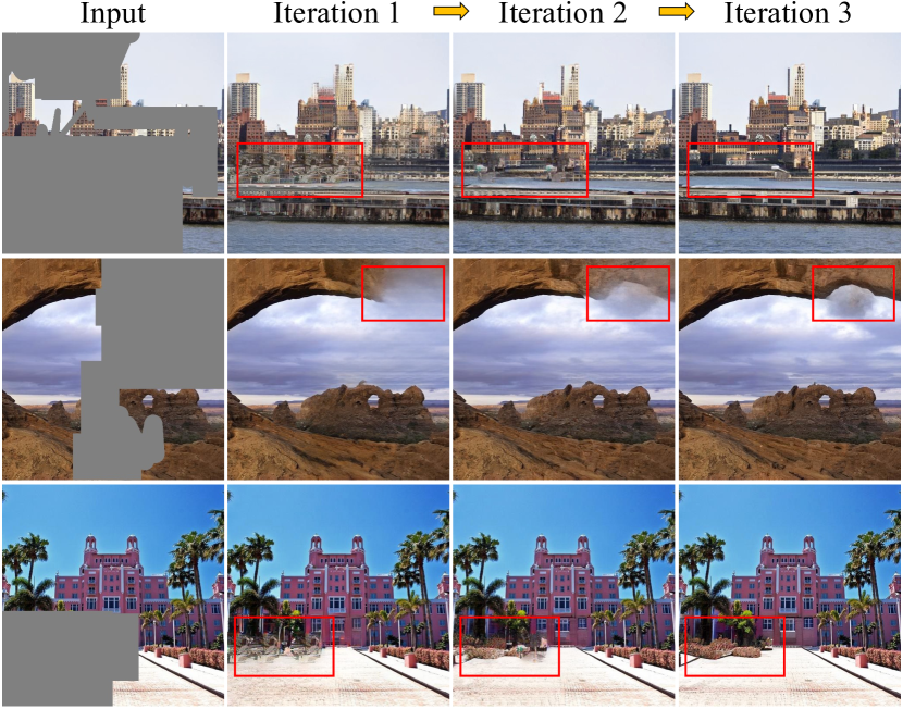
Figure 2: Inpainting results of our PSM at different iterations. One-shot generation usually results in blurry content with unpleasing artifacts, while more iterations yield better results.

To complete the map of inpainting, in this paper, we develop a new pixel spread model (PSM) tailored for the large-hole scenario. PSM operates in an iterative manner, where all pixels are predicted in parallel during each iteration, and only qualified predictions are retained for subsequent iterations. It acts as a process to gradually spread trustful pixels to unknown locations. Our core design lies in a simple yet highly effective decoupled probabilistic modeling (see Sec. 3.1.1), which enjoys the merits of GANs’ efficient optimization and the tractability of probabilistic models. In detail, our model simultaneously predicts an inpainted result (i.e., the mean term) and an uncertainty map (i.e., the variance term). The mean term is optimized using implicit adversarial training, yielding more accurate predictions with fewer iterations. The variance term, contrarily, is modeled explicitly using Gaussian regularization.

The adoption of our decoupled strategy offers numerous advantages. First, the use of adversarial optimization leads to a significant reduction in the number of iterative steps required to achieve promising results, as shown in Fig. 2, much faster than autoregressive and denoising diffusion models. Second, the Gaussian regularization employed produces a variance term that naturally acts as an uncertainty measure (see Sec. 3.1.2). This allows for the selection of reliable estimates for iterative refinement, largely reducing GANs’ artifacts. Furthermore, the explicit modeling of the distribution facilitates continuous sampling, thereby producing predictions with enhanced quality and diversity, as demonstrated in Sec. 4. Finally, the uncertainty measure is instrumental in constructing an uncertainty-guided attention mechanism (see Sec. A), which encourages the network to leverage more informative pixels for efficient reasoning. As a result, our PSM completes large missing regions with photo-realistic content, as illustrated in Fig. Image Inpainting via Iteratively Decoupled Probabilistic Modeling.

Our contributions can be summarized as follows:

• We develop a novel pixel spread model (PSM) customized for large-hole image inpainting. Thanks to the proposed iteratively decoupled probabilistic modeling, our model achieves efficient optimization and high-quality completion.

• Our method reaches cutting-edge performance on both Places [82] and CelebA-HQ [23] benchmark datasets. Notably, our PSM outperforms popular denoising diffusion models, e.g., LDM [46], by a large margin, yielding 1.1 FID improvement on Places2 [82] while being significantly more light-weighted (only 20% parameters, $10\times$ faster).

2 Related Work

2.1 Traditional Methods

Image inpainting is a classical computer vision problem. Early methods make use of image priors, such as self-similarity and sparsity. Diffusion-based methods [5, 2], for instance, convey information to the holes from nearby undamaged neighbors. Another line of exemplar-based approaches [16, 55, 29, 9, 12, 31] looks for highly similar patches to complete missing regions using human-defined distance metrics. The most representative work is PatchMatch [3], which employs heuristic searching in a multi-scale image space to speed up inpainting greatly. However, due to a lack of context understanding, they do not guarantee visually appealing and semantically consistent results.

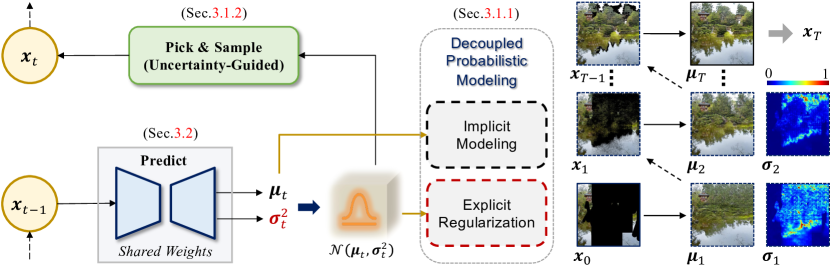
Figure 3: Our pixel spread model for high-quality large-hole image inpainting. Left illustration is the pixel spread pipeline with proposed decoupled probabilistic modeling, and the right images are visual examples. We simplify the input of the $t$-th iteration to $\boldsymbol{x}_{t-1}$, and denote the estimated mean and variance as $\boldsymbol{\mu}_{t}$ and $\boldsymbol{\sigma}^{2}_{t}$. The $\boldsymbol{\sigma}_{t}$ map on the right is normalized for better visualization. We observe gradual uncertainty reduction in missing regions during the pixel spread process.

2.2 Deep Learning Based Methods

Using a great amount of training data to considerably increase the ability of high-level understanding, deep-neural-network-based methods [43, 69, 75, 36, 64] achieve success. Pathak et al. [43] introduce the adversarial loss [13] to inpainting, yielding visually realistic results. Several approaches along this line continually push the performance to new heights. For example, in order to obtain locally fine-grained details and globally consistent structures, Iizuka et al. [20] adopt two discriminators for adversarial training. Additionally, partial [35] and gated [72] convolution layers are proposed to reduce artifacts, e.g., color discrepancy and blurriness, for irregular masks. Moreover, intermediate cues, including foreground contours [68], object structures [40, 45], and segmentation maps [54] are used in multi-stage generation. Despite nice inpainting content for small masks, these methods still do not guarantee large-hole inpainting quality.

2.3 Large Hole Image Inpainting

To deal with large missing regions, a surge of effort was made to improve the model capability. Attention techniques [71, 37, 67, 70] and transformer architectures [62, 81, 34] take advantage of context information. They work well when an image contains repeating patterns. Besides, Zhao et al. [80] propose a novel architecture, bridging the gap between image-conditional and unconditional generation, improving free-form large-scale image completion. There are also attempts to study the progressive generation. This line is to select only high-quality pixels each time and gradually fill holes. We note that these methods heavily rely on specially designed update algorithms [78, 15, 33, 41], or consume additional model capacity to separately assess the prediction accuracy [77], or need more training stages [7] when processing images.

Recently, benefiting from exact likelihood computation and iterative samplings, autoregressive models [62, 74, 66] and denoising diffusion models [48, 46, 38, 1] have shown great potential in producing diversified and realistic content. They inevitably incur high inference costs with thousands of steps and require massive computation resources. In this work, we present decoupled probabilistic modeling that obtains predictions and uncertainty measures simultaneously. Our model identifies reliable predicted pixels and sends them to subsequent iterations, thereby mitigating GANs-generated artifacts. Also, the proposed approach can be viewed as a diffusion model that learns pixel spreading rather than denoising and requires fewer iterations.

3 Our Method

Our objective is to use photo-realistic material to complete a masked image with substantial missing areas. In this section, we first formulate our pixel spread model (PSM) along with a comprehensive analysis. It is followed by the details of model design and loss functions.

3.1 Pixel Spread Model

Although GANs-based methods achieve significantly better results than traditional ones, they still face great difficulties handling large missing regions. We attribute one of the reasons to the one-shot nature of GANs and instead propose iterative inpainting.

In each pass, since there are inevitably some good predictions, we use these pixels as clues to assist the next-time generation. In this way, our pixel spread model gradually propagates valuable information to the entire image. In the following, we first discuss the single-pass modeling before moving on to the pixel spread process.

3.1.1 Decoupled Probabilistic Modeling

For iterative inpainting, it is essential to find a mechanism to evaluate the accuracy of predictions. One intuitive solution is introducing a tractable probabilistic model so that uncertainty information can be analytically calculated. However, this requirement often leads to the assumption that the approximated target distribution is Gaussian, which is considerably too simple to explain the truly complicated distributions. Although several iterative models, such as denoising diffusion models [19], enrich the expression of marginal distribution by including a number of hidden variables and optimizing the variational lower evidence bound, these methods typically yield a high inference cost.

To address these key issues, we propose a decoupled probabilistic modeling tailored for efficient iterative inpainting. The essential insight is that we leverage the advantages of implicit GANs-based optimization and explicit Gaussian regularization in a decoupled way. Thus we can simultaneously obtain accurate predictions and explicit uncertainty measures.

As shown in Fig. 3, given an input image $\boldsymbol{x}_{t}$ at time $t$ with large holes, our model (see architecture details in Sec. A) predicts the inpainting result $\boldsymbol{\mu}_{t}$ as well as an uncertainty map $\boldsymbol{\sigma}_{t}^{2}$. We use the adversarial loss (along with other losses of Sec. 3.3) to supervise image prediction $\boldsymbol{\mu}_{t}$, while jointly treating $(\boldsymbol{\mu}_{t},\boldsymbol{\sigma}_{t}^{2})$ as the mean and diagonal covariance of Gaussian distribution. GANs’ implicit optimization makes it possible to approximate the true distribution as closely as possible, greatly reducing the number of iterations. It also supplies us with an explicit uncertainty measure for the mean term, allowing us to select reliable pixels. The Gaussian regularization is mainly applied to the variance term using negative log likelihood (NLL) $\mathcal{L}_{nll}$ as

$$\small\mathcal{L}_{nll}=-\sum_{i=1}^{D}\log\int_{\delta_{-}(\boldsymbol{y}^{i})}^{{\delta_{+}(\boldsymbol{y}^{i})}}\mathcal{N}\left(y;{\rm sg}[\boldsymbol{\mu}^{i}_{\theta}(\boldsymbol{x})],{\boldsymbol{\sigma}^{i}_{\theta}}(\boldsymbol{x})^{2}\right)dy\,,$$ (1)

where $D$ is the data dimension and $i$ is the pixel index, $\theta$ denotes model parameters, and input $\boldsymbol{x}$ and output $\boldsymbol{y}$ are scaled to $[-1,1]$. $\delta_{+}(y)$ and $\delta_{-}(y)$ are defined as

$$\delta_{+}(y) =\left\{\begin{array}[]{cl}\infty&{\rm if}\ y\ =\ 1\,,\\ y+\frac{1}{255}&{\rm if}\ y\ <\ 1\,,\end{array}\right.$$ (4)

$$\delta_{-}(y) =\left\{\begin{array}[]{cl}-\infty&{\rm if}\ y\ =\ -1\,,\\ y-\frac{1}{255}&{\rm if}\ y\ >\ -1\,.\end{array}\right.$$ (7)

Specifically, we include a stop-gradient operation (i.e., ${\rm sg[\cdot]}$), which encourages the Gaussian constraint only to optimize the variance term and allows the mean term to be estimated from more accurate implicit modeling.

Discussion. We use the estimated mean and variance for sampling during the diffusion process, while taking the deterministic mean term as the output for the final iteration. The feasibility of this design is proved by the experiments in Sec. 4. Additionally, the probabilistic modeling enables us to apply continuous sampling during pixel spread, yielding higher quality and more diverse estimations. Finally, we find the uncertainty measure also enables us to design a more effective attention mechanism in Sec. A.

3.1.2 Pixel Spread Scheme

We use a feed-forward network, denoted as $f_{\theta}(\cdot)$, to gradually spread informative pixels to the entire image, starting from known regions as

$$\boldsymbol{x}_{t},\boldsymbol{m}_{t},\boldsymbol{u}_{t}=f_{\theta}(\boldsymbol{x}_{t-1},\boldsymbol{m}_{t-1},\boldsymbol{u}_{t-1})\,,$$ (8)

where $t$ is the time step, $\boldsymbol{x}_{t}$ refers to the masked image, $\boldsymbol{m}_{t}$ stands for a binary mask, and $\boldsymbol{u}_{t}$ is the uncertainty map. The output includes the updated image, mask, and uncertainty map. Network parameters are shared across all iterations.

We use several iterations for both training and testing to improve performance. Specifically, as shown in Fig. 3 and Eq. (8), our method runs as follows at the $t$-th iteration.

1. Predict. Given the masked image $\boldsymbol{x}_{t-1}$, mask $\boldsymbol{m}_{t-1}$, and uncertainty map $\boldsymbol{u}_{t-1}$, our method estimates mean $\boldsymbol{\mu}_{t}$ and variance $\boldsymbol{\sigma}^{2}_{t}$ for all pixels. Then a preliminary uncertainty map $\tilde{\boldsymbol{u}}_{t}$ scaled to $\left[0,1\right]$ is generated by converting the variance map.

2. Pick. We first sort the uncertainty scores for unknown pixels. According to the pre-defined mask schedule, we calculate the number of pixels that are to be added in this iteration, and insert those with the lowest uncertainty to the known category, updating the mask to $\boldsymbol{m}_{t}$. Based on the preliminary uncertainty map $\tilde{\boldsymbol{u}}_{t}$, by marking locations that are still missing as 1 and the initially known pixels as 0, we obtain the final uncertainty map $\boldsymbol{u}_{t}$.

3. Sample. We consider two situations. First, for the initially known locations $\boldsymbol{m}_{0}$, we always use the original input pixels $\boldsymbol{x}_{0}$. Second, we apply continuous sampling in accordance with $\boldsymbol{\mu}_{t}$ and $\boldsymbol{\sigma}_{t}$ for the inpainting areas. The result is formulated as

   $$\boldsymbol{x}_{t}=\boldsymbol{x}_{0}+(\boldsymbol{m}_{t}-\boldsymbol{m}_{0})\odot(\boldsymbol{\mu_{t}}+\alpha\cdot\boldsymbol{\sigma}_{t}\odot\boldsymbol{z})\,,$$ (9)

   where $\alpha$ is an adjustable ratio and $\boldsymbol{z}\sim\mathcal{N}(\boldsymbol{0},\boldsymbol{I})$, and $\odot$ denotes the Hadamard product. Note that we do not use the $\boldsymbol{\sigma}_{t}\boldsymbol{z}$ term in the final iteration.

3.2 Model Architecture

We use a deep U-Net [47] architecture with a StyleGAN [25, 26] decoder, reaching large receptive fields with stacked convolutions to take advantage of context information in images [6, 39, 4, 63]. In addition, we introduce multiple attention blocks at various resolutions, in light of the discovery that global interaction significantly improves reconstruction quality on much larger and more diverse datasets at higher resolutions [71, 70, 11].

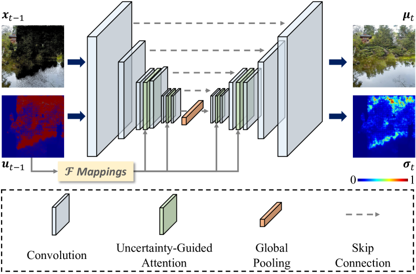
Figure 4: U-Net architecture with the proposed uncertainty-guided attention. We omit the mask update for clarity.

Based only on feature similarity, the conventional attention mechanism [59] offers equal opportunity for pixels to exchange information. For the inpainting task, however, missing pixels are initialized with the same specified values, making them close to one another. As a result, it is usually unable to effectively leverage useful information from visible regions. Even worse, the valid pixels are compromised, resulting in blurry content and unpleasing artifacts.

In this situation, as shown in Fig. 4, we take into account the pixels’ uncertainty scores to adjust the aggregating weights in attention. It properly resolves the problem mentioned above. The attention output is computed by

$${\rm Attention}(\boldsymbol{q},\boldsymbol{k},\boldsymbol{v},\boldsymbol{u})={\rm Softmax}\left(\frac{\boldsymbol{q}\boldsymbol{k}^{T}}{\sqrt{d_{k}}}+\mathcal{F}(\boldsymbol{u})\right)\boldsymbol{v}\,,$$ (10)

where $\{\boldsymbol{q},\boldsymbol{k},\boldsymbol{v}\}$ are the query, key, value matrices, $d_{k}$ denotes the scaling factor, and $\mathcal{F}$ represents learnable functions that predict biased pixel weights based on the uncertainty map $\boldsymbol{u}$ and also include a reshape operation.

3.3 Loss Functions

In each iteration, our model outputs the mean and variance estimates, as shown in Fig 3. The mean term is optimized using adversarial loss [13] $\mathcal{L}_{adv}$ and perceptual loss [56, 22] $\mathcal{L}_{pcp}$, which aims to produce natural-looking images. The losses are described as follows.

Adversarial loss. We formulate the adversarial loss as

$$\mathcal{L}_{ag} =-\mathbb{E}_{\hat{x}}\left[\log\left(D\left(\hat{x}\right)\right)\right]\,,$$ (11)

$$\mathcal{L}_{ad} =-\mathbb{E}_{x}\left[\log\left(D\left(x\right)\right)\right]-\mathbb{E}_{\hat{x}}\left[\log\left(1-D\left(\hat{x}\right)\right)\right]\,,$$ (12)

where $D$ is the discriminator implemented as [25], $x$ and $\hat{x}$ are real and predicted images.

Perceptual loss. We adopt a high receptive filed perceptual loss [56], which is formulated as

$$\mathcal{L}_{pcp}=\sum_{i}\left\|\phi_{i}(x)-\phi_{i}(\hat{x})\right\|^{2}_{2}\,,$$ (13)

where $\phi_{i}$ is the layer output of a pre-trained ResNet50 [17].

As discussed in Sec. 3.1.1, we apply the negative log likelihood $\mathcal{L}_{nll}$ to constrain the variance for uncertainty modeling. Thus the final loss function for the generator is

$$\mathcal{L}=\sum\nolimits_{j}\lambda_{1}\mathcal{L}_{ag}^{j}+\lambda_{2}\mathcal{L}_{pcp}^{j}+\lambda_{3}\mathcal{L}_{nll}^{j},$$ (14)

where $j$ is the number of spread iterations. We empirically set $\lambda_{1}=1$, $\lambda_{2}=2$ and $\lambda_{3}$ to $1\times 10^{-4}$.

4 Experiments

4.1 Datasets and Metrics

We train our models at $512\times 512$ resolution on Places2 [82] and CelebA-HQ [23] in order to adequately assess the proposed method. Places2 is a large-scale dataset with nearly 8 million training images in various scene categories. Additionally, 36,500 images make up the validation split. During training, images undergo random flipping, cropping, and padding, while testing images are centrally cropped to the $512\times 512$ size. For CelebA-HQ, we employ 24,183 and 2,993 images, respectively, to train and test our models. Following [72, 80, 56, 34], we use on-the-fly generated masks during training, where the detailed setup is from MAT [34]. We evaluate all models using identical masks provided by [34] for fair comparisons. Besides, for evaluating model robustness, we use the same model to inpaint both small and large masks.

Despite being adopted in early inpainting work, L1 distance, PSNR, and SSIM [65] are found not strongly associated with human perception when assessing image quality [30, 50]. In this work, in light of [80, 34], we use FID [18], P-IDS [80], and U-IDS [79], which robustly measures the perceptual fidelity of inpainted images, as more suitable metrics.

4.2 Implementation Details

We use an encoder-decoder architecture. The encoder is made up of convolution blocks, while the decoder is adopted from StyleGAN2 [26]. The encoder’s channel size starts at 64 and doubles after each downsampling until the maximum of 512. The decoder has a symmetrical configuration. We adopt attention blocks at $32\times 32$ and $16\times 16$ resolutions for both the encoder and decoder. The uncertainty map is initialized as “1 - mask” at the first iteration. Given an $H\times W$ input, we first downsample the feature size to $\frac{H}{32}\times\frac{W}{32}$ before returning to $H\times W$.

We train our models for 20M images on Places2 and CelebA-HQ using 8 NVIDIA A100 GPUs. We utilize exponential moving average (EMA), adaptive discriminator augmentation (ADA), and weight modulation training strategies [24, 34]. The batch size is 32, and the learning rate is $1\times 10^{-3}$. We employ an Adam [27] optimizer with $\beta_{1}=0$ and $\beta_{2}=0.99$. We empirically set $\alpha=0.01$ in Eq. (9) based on experimental results. To generate $512\times 512$ images, we iterate twice for training and four times for testing.

The fact that previous work [80, 34] trains models on Places2 with 50M or more images – much more extensive data than ours – evidences the benefit of our method. It is found that additional training can further improve our approach, and yet 20M images currently already deliver cutting-edge performance.

4.3 Ablation Study

Model	Iter.	DPM	CS	UGA	Att. Res.	FID$\downarrow$
A	3	✓	✓	✓	32,16	2.36
B	1	-	-	✓	32,16	2.95
C	2	✓	✓	✓	32,16	2.55
D	3		✓	✓	32,16	2.49
E	3	✓		✓	32,16	2.45
F	3	✓	✓		32,16	2.44
G	3	✓	✓	✓	16	2.64

Table 1: Quantitative ablation study of the number of training iterations, modeling and sampling strategies, and architecture designs. Model “A” refers to the full model. Models “B” and “C” use fewer iterations. We tease apart the decoupled probabilistic modeling (DPM), continuous sampling (CS), and uncertainty-guided attention (UGA) in models “D”, “E”, and “F”. Model “G” only adopts attention blocks at $16\times 16$ resolution.

Iter.	4	5	6	7	8	9	10
Model A	2.23	2.16	2.12	2.09	2.07	2.05	2.05
Model B	2.27	2.20	2.16	2.14	2.12	2.11	2.11

Table 2: Quantitative ablation study of the number of testing iterations. As the number of iterations increases, the FID$\downarrow$ results get better and then saturate.

In this section, we conduct a comprehensive investigation of the proposed designs in our method. For quick evaluation, we train our models for 6M images at $256\times 256$ resolution using Places365-Standard, a subset of Places2 [82]. We start with model “A”, which employs our full designs and adopts three iterations during training.

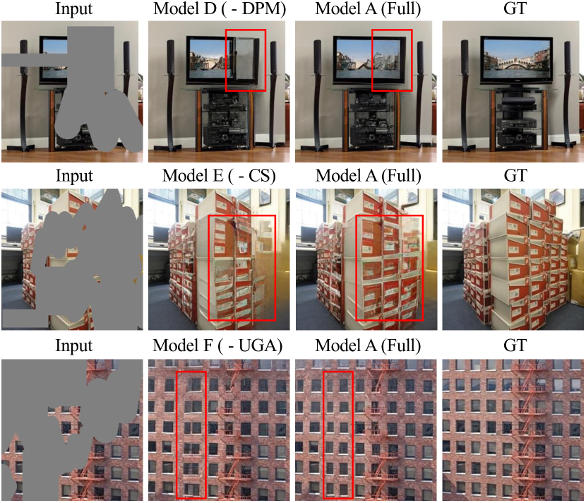
Figure 5: Qualitative ablation study. Model “A” is our full model. The proposed decoupled probabilistic modeling, continuous sampling, and uncertainty-guided attention designs are not used in models “D”, “E”, and “F”.

Iterative number. Our core idea is to employ iterative optimization to enhance the generation quality. We adjust the iteration number and maintain the same setup during training and testing. As illustrated in Table 1, models with one and two iterations, dubbed “B” and “C”, yield 0.59 and 0.19 FID decreases compared to model “A”. Additionally, as shown in Fig. 2, adopting more iterations is capable of producing more aesthetically pleasing content. The first and third cases exhibit obviously fewer artifacts, and the arch in the second example is successfully restored after three iterations. Both the quantitative and qualitative results manifest the importance of iterative generation.

Method	#Param. $\times 10^{6}$	Places2 ($512\times 512$)						CelebA-HQ ($512\times 512$)
		Small Mask			Large Mask			Small Mask			Large Mask
		FID$\downarrow$	P-IDS($\%$)$\uparrow$	U-IDS($\%$)$\uparrow$	FID$\downarrow$	P-IDS($\%$)$\uparrow$	U-IDS($\%$)$\uparrow$	FID$\downarrow$	P-IDS($\%$)$\uparrow$	U-IDS($\%$)$\uparrow$	FID$\downarrow$	P-IDS($\%$)$\uparrow$	U-IDS($\%$)$\uparrow$
PSM (ours)	74	0.72	30.95	43.91	1.68	25.33	39.30	2.34	22.42	33.43	4.05	16.10	28.25
Stable Diffusion†	860	1.32	12.69	34.78	2.11	12.01	32.57	-	-	-	-	-	-
LDM [46]	387	1.06	16.23	39.61	2.76	12.11	33.02	-	-	-	-	-	-
MAT [34]	62	1.07	27.42	41.93	2.90	19.03	35.36	2.86	21.15	32.56	4.86	13.83	25.33
CoModGAN [80]	109	1.10	26.95	41.88	2.92	19.64	35.78	3.26	19.65	31.41	5.65	11.23	22.54
LaMa [56]	51/27	0.99	22.79	40.58	2.97	13.09	32.29	4.05	9.72	21.57	8.15	2.07	7.58
ICT [62]	150	-	-	-	-	-	-	6.28	2.24	9.99	12.84	0.13	0.58
MADF [83]	85	2.24	14.85	35.03	7.53	6.00	23.78	3.39	12.06	24.61	6.83	3.41	11.26
AOT GAN [76]	15	3.19	8.07	30.94	10.64	3.07	19.92	4.65	7.92	20.45	10.82	1.94	6.97
HFill [70]	3	7.94	3.98	23.60	28.92	1.24	11.24	-	-	-	-	-	-
DeepFill v2 [72]	4	3.02	9.17	32.56	9.27	4.01	21.32	10.11	3.11	9.52	24.42	0.17	0.42
EdgeConnect [40]	22	4.03	5.88	27.56	12.66	1.93	15.87	10.58	4.14	12.45	39.99	0.10	0.22

Table 3: Quantitative comparisons on Places [82] and CelebA-HQ [23]. “$\dagger$”: the officially released Stable Diffusion inpainting model trained on a large-scale high-quality dataset LAION-Aesthetics V2 5+. Our method achieves the best performance under both large and small mask settings. The best and second best results are in red and blue.

It is noted that we can test the system with a different number of iterations from the training stage. Using more iterations results in higher FID performance, as demonstrated in Table 2, yet at the expense of longer inference time. Thus, there is a trade-off between inference speed and generation quality. Additionally, when comparing models “A” and “B”, it is clear that introducing more iterations in the training process is beneficial. But the number of iterations in the inference stage is more important.

Decoupled probabilistic modeling. To deliver accurate prediction while supporting the uncertainty measure for iterative inpainting, we propose decoupled probabilistic modeling. When putting all supervision on the sampled result, we observe the training diminishes the variance term (close to 0 for all pixels). It is because, unlike denoising diffusion models that precisely quantify the noise levels at each step, our GANs-based method no longer provides specific optimization targets for the mean and variance terms. The variance term is underestimated for trivial optimization in this case. It renders the picking process less effective.

As illustrated in Table 1, model “D” obtains an inferior FID result compared with the full model “A”. Besides, from the visual comparison in Fig. 5, it is observed that model “D” tends to generate blurry content, while model “A” produces sharper structures and fine-grained details. All these observations prove the effectiveness of this design.

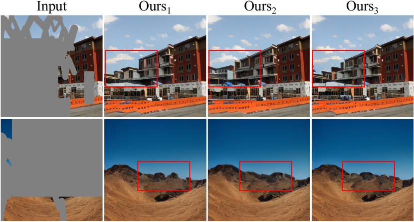
Figure 6: Visual examples of diverse generation for our method. The differences mainly lie in the fine-grained details.

Continuous sampling. Our approach may use the estimated variance to perform continuous sampling. Table 1 indicates that FID decreases by nearly 0.1 when continuous sampling (model ”E”) is not involved. Also, it is observed that our full model leads to more visually consistent content. For example, box structures are well restored according to the visible pixels in Fig. 5. Thus, continuous sampling brings higher fidelity to our results. As shown in Fig. 6, our model also supports the pluralistic generation, particularly in the hole’s center. However, when the mean term is estimated with low uncertainty or the iteration number is constrained, the differences in results are not always instantly obvious. A detailed analysis of fidelity-diversity trade-off is further provided in the supplementary file.

Uncertainty-guided attention. To fully exploit distant context, we add attention blocks to our framework. We first compare using attention at $32\times 32$, $16\times 16$ (model “A”) and only at $16\times 16$ (model “G”). We discover a 0.28 FID drop in model “G” from the quantitative comparison in Table 1, demonstrating the significance of long-range interaction in large-hole image inpainting.

Besides, as aforementioned in Sec. A, the conventional attention mechanism may result in color consistency and blurriness. To support this claim, we tease apart the uncertainty guidance and notice a minor performance drop in Table 1. Also, we provide a visual comparison in Fig. 5. We observe that model “A” produces more visually appealing window details than model “F”.

Mask schedule. As illustrated in Table 4 and Fig. 4, we analyze various mask schedule strategies and discover that the uniform strategy achieves the best FID. We argue that this is because the mask ratios of input images vary widely, and uniform schedule results in more stable training for different iterations.

Mask Sche.	Iter.	FID$\downarrow$
Cubic	3	2.54
Cosine	3	2.48
Linear	3	2.36
Square Root	3	2.47

Table 4: Ablation study of mask schedule functions.

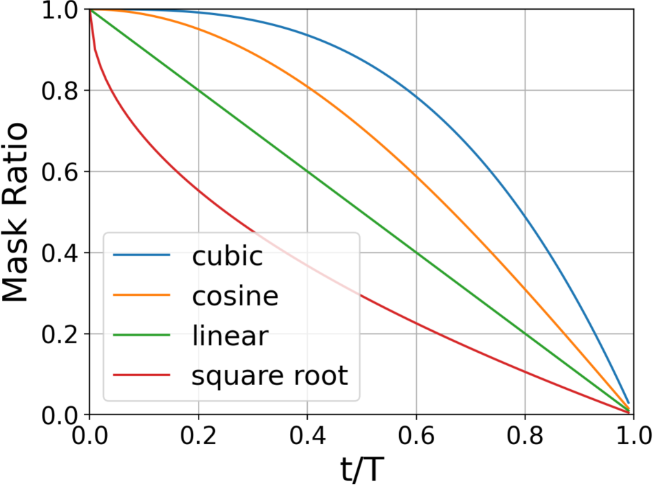
Figure 7: Visualization of mask schedule functions.

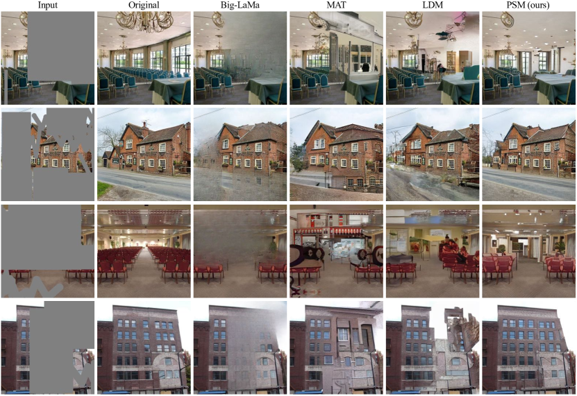
Figure 8: Qualitative side-by-side comparisons of state-of-the-art methods on $512\times 512$ Places2. Our PSM produces structures and details that are more realistic and reasonable.

4.4 Comparisons to State-of-the-Art Methods

We thoroughly compare the proposed pixel spread model (PSM) with GANs-based models [34, 80, 56, 83, 76, 70, 72], autoregressive models [62], and denoising diffusion models [46] in Table 3. Although the last two lines have lately made notable progress even for commercial use, the majority of off-the-shelf techniques can only handle images with up to $256\times 256$ resolution. We use publicly accessible models for $512\times 512$ resolution and test them on the same masks to make a fair comparison.

As shown in Table 3, our PSM achieves the state-of-the-art performance on Places2 and CelebA-HQ benchmarks under both large and small mask settings. It can be seen that our method significantly performs better than the existing GANs-based models. Besides, even with only $20\%$ of the parameters of strong denoising diffusion model LDM [46], our method delivers superior results in terms of all metrics. For example, on the Places2 benchmark, our PSM brings about 1.1 improvement on FID and larger gains on P-IDS and U-ID under the large mask setup. As for the inference speed, our PSM costs nearly 250ms to obtain a $512\times 512$ image, which is $10\times$ faster than LDM ($\sim$3s). Notably, our model is trained using far fewer samples (our 20M images vs. CoModGAN’s [80] 50M images). We observe that more extended training can further boost performance. All these results demonstrate the effectiveness of our method.

We also provide visual comparisons in Fig. 8. In a variety of scenes, our method generates more aesthetically pleasing textures with fewer artifacts when compared to existing methods. For instance, room layouts and building structures are better inpainted by our approach. More examples are provided in the supplementary materials.

5 Conclusion

We have proposed a new pixel spread model for large-hole image inpainting. Utilizing the proposed iteratively decoupled probabilistic modeling, our method can assess the prediction accuracy and retain the pixels with the lowest uncertainty as hints for subsequent processing, yielding high-quality completion. Furthermore, our approach exhibits favorable inference efficiency, significantly surpassing that of prevalent denoising diffusion models. The state-of-the-art performance on multiple benchmarks demonstrate the effectiveness of our method. Additionally, our model has potential for extension to other tasks, such as text-to-image generation, which we will explore in the future.

Limitation analysis. Our method shows a tendency to make more changes in small details rather than in large structures. We aim to improve the diversity of our generation in this regard. Additionally, our method sometimes struggles to understand objects when only a few hints are given, as illustrated by a few failure cases presented in the supplemental materials.

Image Inpainting via Iteratively Decoupled Probabilistic Modeling
(Supplementary Material)

A Architecture Details

Apart from the descriptions in Sec. 3.2 and Sec. 4.2, we here provide a more through illustration of architecture details. We adopt a U-Net architecture with skip connections, where the encoder downsamples the size of an $H\times W$ input to $\frac{H}{32}\times\frac{W}{32}$ and the decoder upsamples it back to $H\times W$. At each resolution, there is just one residual block made up of two $3\times 3$ convolutional layers, unless otherwise stated. Both the encoder and the decoder employ attention blocks at feature sizes of $\frac{H}{16}\times\frac{W}{16}$ and $\frac{H}{32}\times\frac{W}{32}$, and an early convolutional block is also introduced at these scales. Different attention blocks use adaptive mapping functions in Fig. 4, each of which is composed of 4 convolutional layers with a kernel size of $3\times 3$.

The input consists of 7 channels: 3 for color images, 1 for the initial mask, 1 for the updated mask, 1 for the uncertainty map, and 1 for the time step. The number of channels is initially converted to 64, then doubled after each downsampling, up to a maximum of 512, and the decoder employs a symmetrical setup. The output contains 6 channels: 3 for the mean term and 3 for the log variance term.

We use a weight modulation technique, where the style representation is derived from an image global feature and a random latent code. As for the global feature, we employ convolutional layers to further downsample the feature size from $\frac{H}{32}\times\frac{W}{32}$ to $\frac{H}{256}\times\frac{W}{256}$ and a global pooling layer to obtain 1$d$ representation. The random latent code is mapped from Gaussian noise by 8 fully connected layers.

B Generalization to 1024$\times$1024 Resolution

To evaluate the generalization ability of models, we compare our pixel spread model (PSM), MAT [34] and LaMa [56] trained on $512\times 512$ Places2 [82] at the $1024\times 1024$ resolution. As illustrated in Table B.1, our PSM performs significantly better than MAT and LaMa on all metrics, despite using fewer training samples. Remarkably, our approach results in an approximately 1.9 FID improvement. We do not involve denoising diffusion models (e.g., LDM) and other GANs-based models (e.g., CoModGAN) for comparisons because scaling them up to the $1024\times 1024$ resolution is impractical.

Method	FID$\downarrow$	P-IDS($\%$)$\uparrow$	U-IDS($\%$)$\uparrow$
PSM (Ours)	3.95	14.40	32.23
MAT [34]	5.83	9.51	28.02
LaMa [56]	6.31	4.98	23.24

Table B.1: Quantitative comparisons on $1024\times 1024$ Places2 [82] dataset under the large mask setup by transferring models trained at the $512\times 512$ resolution. The best and second best results are in red and blue. Our PSM generalizes well to higher resolutions.

C 512$\times$512 LPIPS Results

Method	#Param.	Places		CelebA-HQ
	$\times 10^{6}$	Small	Large	Small	Large
PSM (Ours)†	74	0.084	0.161	0.052	0.099
Stable Diffusion‡	860	0.148	0.220	-	-
LDM [46]	387	0.100	0.190	-	-
MAT [34]	62	0.099	0.189	0.065	0.125
CoModGAN [80]	109	0.101	0.192	0.073	0.140
LaMa [56]	51/27	0.086	0.166	0.075	0.143
ICT [62]	150	-	-	0.105	0.195
MADF [83]	85	0.095	0.181	0.068	0.130
AOT GAN [76]	15	0.101	0.195	0.074	0.145
HFill [70]	3	0.148	0.284	-	-
DeepFill v2 [72]	4	0.113	0.213	0.117	0.221
EdgeConnect [40]	22	0.114	0.275	0.101	0.208

Table C.2: LPIPS$\downarrow$ results on $512\times 512$ Places2 [82] and CelebA-HQ [23] datasets. “$\dagger$”: our models are trained with 20M samples, much less than other methods (e.g., MAT uses 50M samples on Places2 and 25M samples on CelebA-HQ). We use a single model for both the small and large mask setups. “$\ddagger$”: the official Stable Diffusion inpainting model is trained on a large-scale high-quality dataset LAION-Aesthetics V2 5+. The best and second best results are in red and blue.

LPIPS [79] is also a widely used perceptual metric in image inpainting. For a comprehensive comparison with state-of-the-art methods, we provide LPIPS results in Table C.2. We argue that LPIPS may not be suitable for large-hole image inpainting because it is calculated pixel-by-pixel. This measure is for reference only.

D 256$\times$256 CelebA-HQ Results

We also conduct quantitative comparisons on $256\times 256$ CelebA-HQ [23] dataset. As shown in Table D.3, our method achieves the best performance among all methods.

Method	Small Mask			Large Mask
	FID$\downarrow$	P-IDS$\uparrow$	U-IDS$\uparrow$	FID$\downarrow$	P-IDS$\uparrow$	U-IDS$\uparrow$
PSM (Ours)†	2.58	21.35	33.70	4.57	14.07	25.28
MAT [34]	2.94	20.88	32.01	5.16	13.90	25.13
LaMa [56]	3.98	8.82	22.57	8.75	2.34	8.77
ICT [62]	5.24	4.51	17.39	10.92	0.90	5.23
MADF [83]	10.43	6.25	14.62	23.59	0.50	1.44
AOT GAN [76]	9.64	5.61	14.62	22.91	0.47	1.65
DeepFill v2 [72]	5.69	6.62	16.82	13.23	0.84	2.62
EdgeConnect [40]	5.24	5.61	15.65	12.16	0.84	2.31

Table D.3: Quantitative comparisons on $256\times 256$ CelebA-HQ [23] dataset. The P-IDS and U-IDS results are shown in percentage ($\%$). “$\dagger$”: our model is trained with 12M samples, far less than other methods (e.g., MAT uses 25M samples). We use a single model for both the small and large mask setups. The best and second best results are in red and blue.

E Comparison to RePaint

Considering that the sizes of RePaint [38] results are at $256\times 256$ on Places2 and CelebA-HQ while ours are at $512\times 512$, we don’t compare it in the main body of the paper. Here we compare our model PSM to RePaint at $256\times 256$ resolution on Places2 and CelebA-HQ in Table E.4, where PSM achieves better performance and is $1000\times$ faster than RePaint (i.e., 0.25s v.s. 250s for one image processing). For saving time, we just use the first 10K Places2 validation images for evaluation.

Method	Places2-10K ($256\times 256$)			CelebA-HQ ($256\times 256$)
	FID$\downarrow$	P-IDS($\%$)$\uparrow$	U-IDS($\%$)$\uparrow$	FID$\downarrow$	P-IDS($\%$)$\uparrow$	U-IDS($\%$)$\uparrow$
Ours	3.47	18.32	34.52	4.57	14.07	25.28
RePaint	6.15	11.11	27.16	10.55	0.07	1.47

Table E.4: Quantitative comparisons with RePaint [38] on $256\times 256$ Places [82] and CelebA-HQ [23] datasets.

F Fidelity-Diversity Trade-Off

Apart from FID (depending on both diversity and fidelity), we follow previous work to use Improved Precision and Recall as fidelity (precision) and diversity (recall) measures. As shown in Table F.5, our model yields better FID, higher precision yet slightly lower recall than LDM on Places2, while outperforming MAT on all metrics. Improving diversity will be our future work.

Method	#Param.	FID$\downarrow$	Precision$\uparrow$	Recall$\uparrow$
PSM (Ours)	74M	1.68	0.983	0.971
LDM	387M	2.76	0.962	0.975
MAT	62M	2.90	0.965	0.939

Table F.5: FID, precision and recall comparisons for evaluating fidelity-diversity traed-off on $512\times 512$ Places [82] dataset.

G Additional Pluralistic Generation

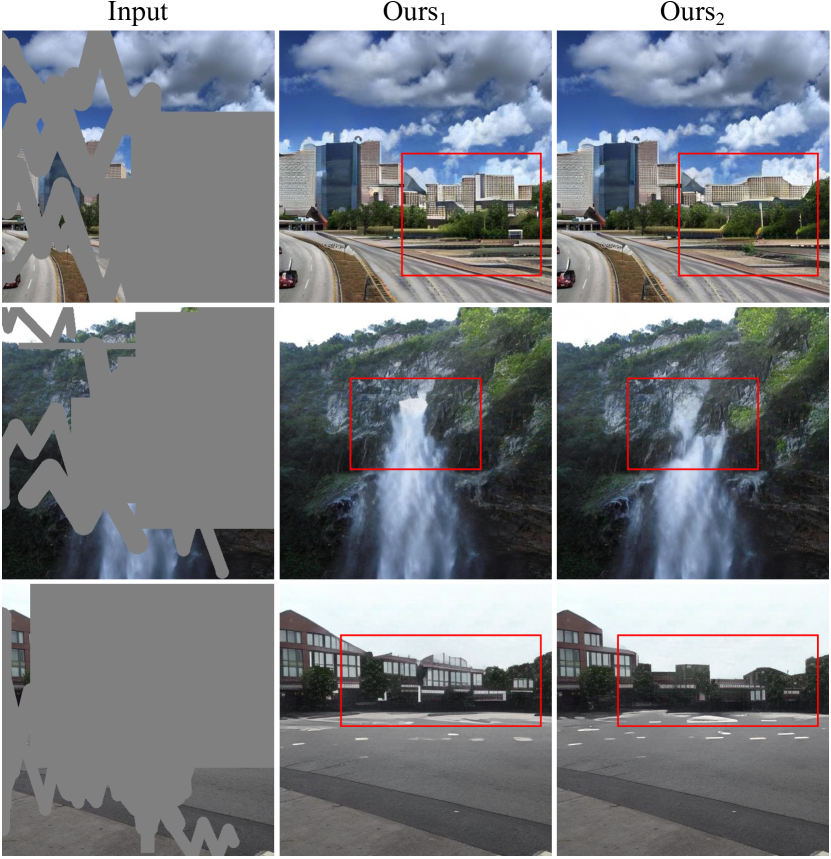
Figure G.1: Visual examples of diverse generation for our method.

As shown in Fig. 6 and Sec. 5, our method also supports pluralistic generation. From the visual examples in Fig. G.1, we observe that the differences mainly lie in the fine-grained details. We will work on improving the generating diversity.

H Additional Qualitative Comparisons

We provide more visual examples on $512\times 512$ Places2 [82] and CelebA-HQ [23] in Fig. H.2, Fig. H.3, Fig. H.4, Fig. H.5, and Fig. H.6. Due to space limit, we additionally add comparisons with CoModGAN [80] in Fig. H.7. Compared to other methods, our method generates more photo-realistic and semantically consistent content. For example, our method successfully recovers human legs, airplane structures, and more realistic indoor and outdoor scenes. All the results demonstrate the effectiveness of our method.

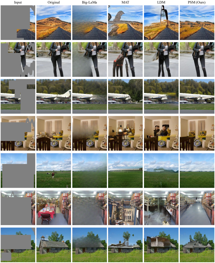
Figure H.2: Qualitative side-by-side comparisons of state-of-the-art methods on $512\times 512$ Places2 dataset. Please zoom in for a better view. Our PSM produces structures and details that are more realistic and reasonable.

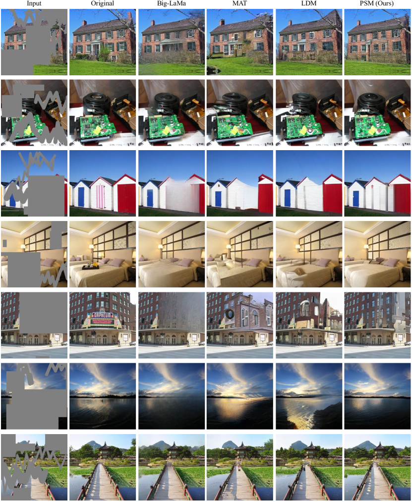
Figure H.3: Qualitative side-by-side comparisons of state-of-the-art methods on $512\times 512$ Places2 dataset. Please zoom in for a better view. Our PSM produces structures and details that are more realistic and reasonable.

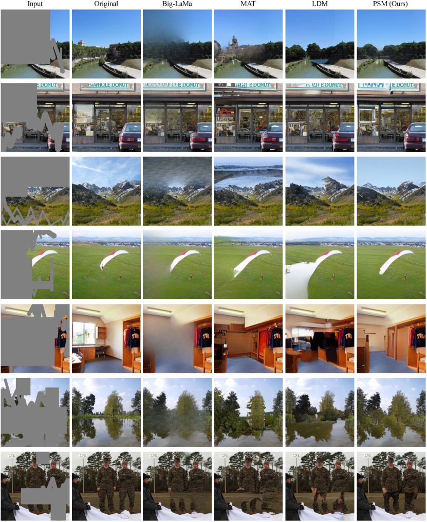
Figure H.4: Qualitative side-by-side comparisons of state-of-the-art methods on $512\times 512$ Places2 dataset. Please zoom in for a better view. Our PSM produces structures and details that are more realistic and reasonable.

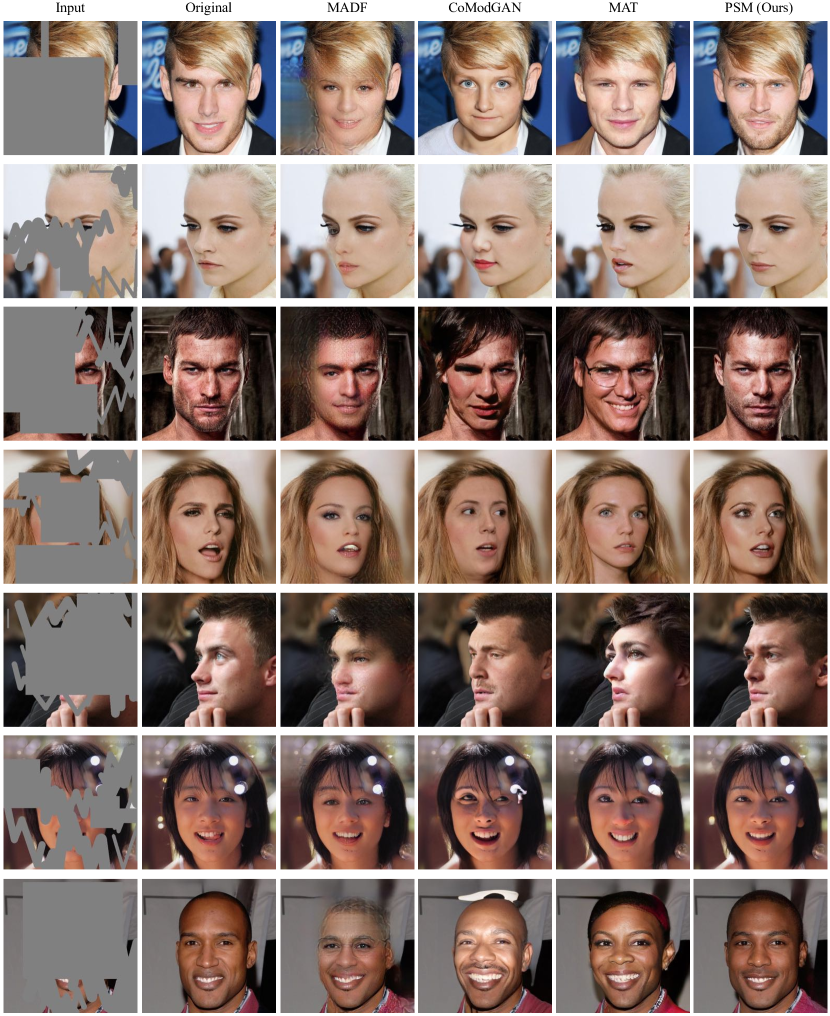
Figure H.5: Qualitative side-by-side comparisons of state-of-the-art methods on $512\times 512$ CelebA-HQ dataset. Please zoom in for a better view. Our PSM produces face outlines and details that are more realistic and reasonable.

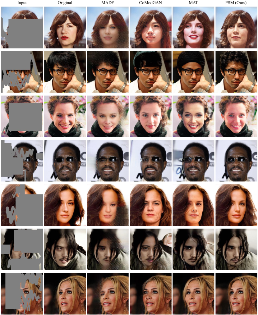
Figure H.6: Qualitative side-by-side comparisons of state-of-the-art methods on $512\times 512$ CelebA-HQ dataset. Please zoom in for a better view. Our PSM produces face outlines and details that are more realistic and reasonable.

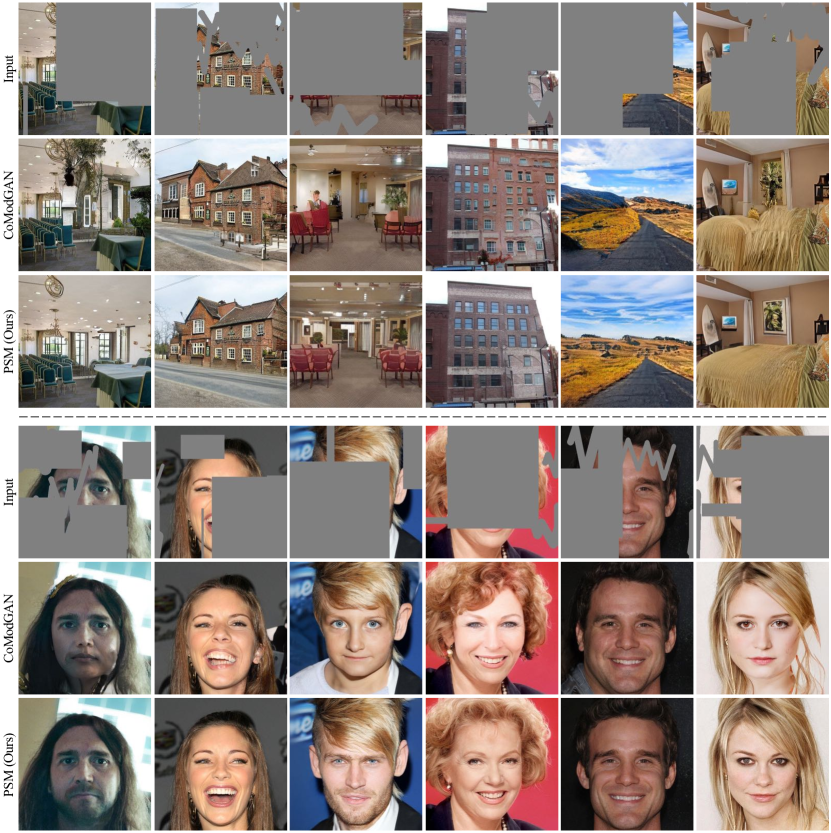
Figure H.7: Qualitative comparisons between CoModGAN and our PSM on $512\times 512$ Places2 and CelebA-HQ datasets. Please zoom in for a better view. Our PSM produces structures and details that are more realistic and reasonable.

I Failure Cases

As discussed in Sec. 5, our model sometimes fails to recover the damaged objects when limited clues are provided. We show some failure cases in Fig. I.8. For instance, the missing part of the notebook is filled with the background, and the recovered bus structure is incomplete. We attribute one of the reasons to the lack of high-level semantic understanding. We will further improve the generative capability of our model.

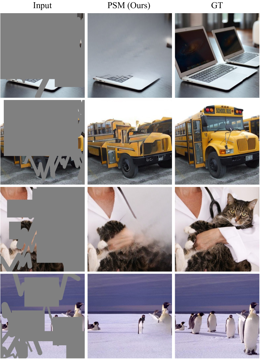
Figure I.8: Failure cases of our PSM. It is difficult to recover the objects when large-scale regions are missing.

References

- [1] Omri Avrahami, Dani Lischinski, and Ohad Fried. Blended diffusion for text-driven editing of natural images. In CVPR, pages 18208–18218, 2022.
- [2] Coloma Ballester, Marcelo Bertalmio, Vicent Caselles, Guillermo Sapiro, and Joan Verdera. Filling-in by joint interpolation of vector fields and gray levels. TIP, 10(8):1200–1211, 2001.
- [3] Connelly Barnes, Eli Shechtman, Adam Finkelstein, and Dan B Goldman. Patchmatch: A randomized correspondence algorithm for structural image editing. TOG, 28(3):24, 2009.
- [4] Dana Berman, Shai Avidan, et al. Non-local image dehazing. In CVPR, pages 1674–1682, 2016.
- [5] Marcelo Bertalmio, Guillermo Sapiro, Vincent Caselles, and Coloma Ballester. Image inpainting. In Proceedings of the 27th annual conference on Computer graphics and interactive techniques, pages 417–424, 2000.
- [6] Antoni Buades, Bartomeu Coll, and J-M Morel. A non-local algorithm for image denoising. In CVPR, volume 2, pages 60–65. IEEE, 2005.
- [7] Huiwen Chang, Han Zhang, Lu Jiang, Ce Liu, and William T Freeman. Maskgit: Masked generative image transformer. In CVPR, pages 11315–11325, 2022.
- [8] Donghyeon Cho, Jinsun Park, Tae-Hyun Oh, Yu-Wing Tai, and In So Kweon. Weakly-and self-supervised learning for content-aware deep image retargeting. In ICCV, pages 4558–4567, 2017.
- [9] Antonio Criminisi, Patrick Perez, and Kentaro Toyama. Object removal by exemplar-based inpainting. In CVPR, volume 2, pages II–II. IEEE, 2003.
- [10] Antonio Criminisi, Patrick Pérez, and Kentaro Toyama. Region filling and object removal by exemplar-based image inpainting. TIP, 13(9):1200–1212, 2004.
- [11] Prafulla Dhariwal and Alexander Nichol. Diffusion models beat gans on image synthesis. NIPS, 34:8780–8794, 2021.
- [12] Ding Ding, Sundaresh Ram, and Jeffrey J Rodríguez. Image inpainting using nonlocal texture matching and nonlinear filtering. TIP, 28(4):1705–1719, 2018.
- [13] Ian Goodfellow, Jean Pouget-Abadie, Mehdi Mirza, Bing Xu, David Warde-Farley, Sherjil Ozair, Aaron Courville, and Yoshua Bengio. Generative adversarial nets. NIPS, 27, 2014.
- [14] Ishaan Gulrajani, Faruk Ahmed, Martin Arjovsky, Vincent Dumoulin, and Aaron C Courville. Improved training of wasserstein gans. NIPS, 30, 2017.
- [15] Zongyu Guo, Zhibo Chen, Tao Yu, Jiale Chen, and Sen Liu. Progressive image inpainting with full-resolution residual network. In ACMMM, pages 2496–2504, 2019.
- [16] James Hays and Alexei A Efros. Scene completion using millions of photographs. ToG, 26(3):4–es, 2007.
- [17] Kaiming He, Xiangyu Zhang, Shaoqing Ren, and Jian Sun. Deep residual learning for image recognition. In CVPR, pages 770–778, 2016.
- [18] Martin Heusel, Hubert Ramsauer, Thomas Unterthiner, Bernhard Nessler, and Sepp Hochreiter. Gans trained by a two time-scale update rule converge to a local nash equilibrium. NIPS, 30, 2017.
- [19] Jonathan Ho, Ajay Jain, and Pieter Abbeel. Denoising diffusion probabilistic models. NIPS, 33:6840–6851, 2020.
- [20] Satoshi Iizuka, Edgar Simo-Serra, and Hiroshi Ishikawa. Globally and locally consistent image completion. ToG, 36(4):1–14, 2017.
- [21] Youngjoo Jo and Jongyoul Park. Sc-fegan: Face editing generative adversarial network with user’s sketch and color. In ICCV, pages 1745–1753, 2019.
- [22] Justin Johnson, Alexandre Alahi, and Li Fei-Fei. Perceptual losses for real-time style transfer and super-resolution. In ECCV, pages 694–711. Springer, 2016.
- [23] Tero Karras, Timo Aila, Samuli Laine, and Jaakko Lehtinen. Progressive growing of gans for improved quality, stability, and variation. In ICLR, 2018.
- [24] Tero Karras, Miika Aittala, Janne Hellsten, Samuli Laine, Jaakko Lehtinen, and Timo Aila. Training generative adversarial networks with limited data. NIPS, 33:12104–12114, 2020.
- [25] Tero Karras, Samuli Laine, and Timo Aila. A style-based generator architecture for generative adversarial networks. In CVPR, pages 4401–4410, 2019.
- [26] Tero Karras, Samuli Laine, Miika Aittala, Janne Hellsten, Jaakko Lehtinen, and Timo Aila. Analyzing and improving the image quality of stylegan. In CVPR, pages 8110–8119, 2020.
- [27] Diederik P Kingma and Jimmy Ba. Adam: A method for stochastic optimization. In ICLR, 2015.
- [28] Naveen Kodali, Jacob Abernethy, James Hays, and Zsolt Kira. On convergence and stability of gans. arXiv preprint arXiv:1705.07215, 2017.
- [29] Olivier Le Meur, Josselin Gautier, and Christine Guillemot. Examplar-based inpainting based on local geometry. In ICIP, pages 3401–3404. IEEE, 2011.
- [30] Christian Ledig, Lucas Theis, Ferenc Huszár, Jose Caballero, Andrew Cunningham, Alejandro Acosta, Andrew Aitken, Alykhan Tejani, Johannes Totz, Zehan Wang, et al. Photo-realistic single image super-resolution using a generative adversarial network. In CVPR, pages 4681–4690, 2017.
- [31] Joo Ho Lee, Inchang Choi, and Min H Kim. Laplacian patch-based image synthesis. In CVPR, pages 2727–2735, 2016.
- [32] Anat Levin, Assaf Zomet, Shmuel Peleg, and Yair Weiss. Seamless image stitching in the gradient domain. In ECCV, pages 377–389. Springer, 2004.
- [33] Jingyuan Li, Ning Wang, Lefei Zhang, Bo Du, and Dacheng Tao. Recurrent feature reasoning for image inpainting. In CVPR, pages 7760–7768, 2020.
- [34] Wenbo Li, Zhe Lin, Kun Zhou, Lu Qi, Yi Wang, and Jiaya Jia. Mat: Mask-aware transformer for large hole image inpainting. In CVPR, pages 10758–10768, 2022.
- [35] Guilin Liu, Fitsum A Reda, Kevin J Shih, Ting-Chun Wang, Andrew Tao, and Bryan Catanzaro. Image inpainting for irregular holes using partial convolutions. In ECCV, pages 85–100, 2018.
- [36] Hongyu Liu, Bin Jiang, Yibing Song, Wei Huang, and Chao Yang. Rethinking image inpainting via a mutual encoder-decoder with feature equalizations. In ECCV, pages 725–741. Springer, 2020.
- [37] Hongyu Liu, Bin Jiang, Yi Xiao, and Chao Yang. Coherent semantic attention for image inpainting. In ICCV, pages 4170–4179, 2019.
- [38] Andreas Lugmayr, Martin Danelljan, Andres Romero, Fisher Yu, Radu Timofte, and Luc Van Gool. Repaint: Inpainting using denoising diffusion probabilistic models. In CVPR, pages 11461–11471, 2022.
- [39] Julien Mairal, Francis Bach, Jean Ponce, Guillermo Sapiro, and Andrew Zisserman. Non-local sparse models for image restoration. In ICCV, pages 2272–2279. IEEE, 2009.
- [40] Kamyar Nazeri, Eric Ng, Tony Joseph, Faisal Z Qureshi, and Mehran Ebrahimi. Edgeconnect: Generative image inpainting with adversarial edge learning. arXiv preprint arXiv:1901.00212, 2019.
- [41] Seoung Wug Oh, Sungho Lee, Joon-Young Lee, and Seon Joo Kim. Onion-peel networks for deep video completion. In ICCV, pages 4403–4412, 2019.
- [42] Niki Parmar, Ashish Vaswani, Jakob Uszkoreit, Lukasz Kaiser, Noam Shazeer, Alexander Ku, and Dustin Tran. Image transformer. In ICML, pages 4055–4064. PMLR, 2018.
- [43] Deepak Pathak, Philipp Krahenbuhl, Jeff Donahue, Trevor Darrell, and Alexei A Efros. Context encoders: Feature learning by inpainting. In CVPR, pages 2536–2544, 2016.
- [44] Aditya Ramesh, Prafulla Dhariwal, Alex Nichol, Casey Chu, and Mark Chen. Hierarchical text-conditional image generation with clip latents. arXiv preprint arXiv:2204.06125, 2022.
- [45] Yurui Ren, Xiaoming Yu, Ruonan Zhang, Thomas H Li, Shan Liu, and Ge Li. Structureflow: Image inpainting via structure-aware appearance flow. In ICCV, pages 181–190, 2019.
- [46] Robin Rombach, Andreas Blattmann, Dominik Lorenz, Patrick Esser, and Björn Ommer. High-resolution image synthesis with latent diffusion models. In CVPR, pages 10684–10695, 2022.
- [47] Olaf Ronneberger, Philipp Fischer, and Thomas Brox. U-net: Convolutional networks for biomedical image segmentation. In International Conference on Medical image computing and computer-assisted intervention, pages 234–241. Springer, 2015.
- [48] Chitwan Saharia, William Chan, Huiwen Chang, Chris Lee, Jonathan Ho, Tim Salimans, David Fleet, and Mohammad Norouzi. Palette: Image-to-image diffusion models. In ACM SIGGRAPH 2022 Conference Proceedings, pages 1–10, 2022.
- [49] Chitwan Saharia, William Chan, Saurabh Saxena, Lala Li, Jay Whang, Emily Denton, Seyed Kamyar Seyed Ghasemipour, Burcu Karagol Ayan, S Sara Mahdavi, Rapha Gontijo Lopes, et al. Photorealistic text-to-image diffusion models with deep language understanding. arXiv preprint arXiv:2205.11487, 2022.
- [50] Mehdi SM Sajjadi, Bernhard Scholkopf, and Michael Hirsch. Enhancenet: Single image super-resolution through automated texture synthesis. In ICCV, pages 4491–4500, 2017.
- [51] Tim Salimans, Ian Goodfellow, Wojciech Zaremba, Vicki Cheung, Alec Radford, and Xi Chen. Improved techniques for training gans. NIPS, 29, 2016.
- [52] Uriel Singer, Adam Polyak, Thomas Hayes, Xi Yin, Jie An, Songyang Zhang, Qiyuan Hu, Harry Yang, Oron Ashual, Oran Gafni, et al. Make-a-video: Text-to-video generation without text-video data. arXiv preprint arXiv:2209.14792, 2022.
- [53] Yang Song and Stefano Ermon. Generative modeling by estimating gradients of the data distribution. NIPS, 32, 2019.
- [54] Yuhang Song, Chao Yang, Yeji Shen, Peng Wang, Qin Huang, and C-C Jay Kuo. Spg-net: Segmentation prediction and guidance network for image inpainting. arXiv preprint arXiv:1805.03356, 2018.
- [55] Jian Sun, Lu Yuan, Jiaya Jia, and Heung-Yeung Shum. Image completion with structure propagation. In ACM SIGGRAPH 2005 Papers, pages 861–868. 2005.
- [56] Roman Suvorov, Elizaveta Logacheva, Anton Mashikhin, Anastasia Remizova, Arsenii Ashukha, Aleksei Silvestrov, Naejin Kong, Harshith Goka, Kiwoong Park, and Victor Lempitsky. Resolution-robust large mask inpainting with fourier convolutions. arXiv preprint arXiv:2109.07161, 2021.
- [57] Aaron Van den Oord, Nal Kalchbrenner, Lasse Espeholt, Oriol Vinyals, Alex Graves, et al. Conditional image generation with pixelcnn decoders. NIPS, 29, 2016.
- [58] Aäron Van Den Oord, Nal Kalchbrenner, and Koray Kavukcuoglu. Pixel recurrent neural networks. In ICML, pages 1747–1756. PMLR, 2016.
- [59] Ashish Vaswani, Noam Shazeer, Niki Parmar, Jakob Uszkoreit, Llion Jones, Aidan N Gomez, Łukasz Kaiser, and Illia Polosukhin. Attention is all you need. In NIPS, pages 5998–6008, 2017.
- [60] Ziyu Wan, Bo Zhang, Dongdong Chen, Pan Zhang, Dong Chen, Jing Liao, and Fang Wen. Bringing old photos back to life. In CVPR, pages 2747–2757, 2020.
- [61] Ziyu Wan, Bo Zhang, Dongdong Chen, Pan Zhang, Dong Chen, Fang Wen, and Jing Liao. Old photo restoration via deep latent space translation. TPAMI, 2022.
- [62] Ziyu Wan, Jingbo Zhang, Dongdong Chen, and Jing Liao. High-fidelity pluralistic image completion with transformers. arXiv preprint arXiv:2103.14031, 2021.
- [63] Xiaolong Wang, Ross Girshick, Abhinav Gupta, and Kaiming He. Non-local neural networks. In CVPR, pages 7794–7803, 2018.
- [64] Yi Wang, Xin Tao, Xiaojuan Qi, Xiaoyong Shen, and Jiaya Jia. Image inpainting via generative multi-column convolutional neural networks. NIPS, 2018.
- [65] Zhou Wang, Alan C Bovik, Hamid R Sheikh, and Eero P Simoncelli. Image quality assessment: from error visibility to structural similarity. TIP, 13(4):600–612, 2004.
- [66] Chenfei Wu, Jian Liang, Xiaowei Hu, Zhe Gan, Jianfeng Wang, Lijuan Wang, Zicheng Liu, Yuejian Fang, and Nan Duan. Nuwa-infinity: Autoregressive over autoregressive generation for infinite visual synthesis. NIPS, 2022.
- [67] Chaohao Xie, Shaohui Liu, Chao Li, Ming-Ming Cheng, Wangmeng Zuo, Xiao Liu, Shilei Wen, and Errui Ding. Image inpainting with learnable bidirectional attention maps. In ICCV, pages 8858–8867, 2019.
- [68] Wei Xiong, Jiahui Yu, Zhe Lin, Jimei Yang, Xin Lu, Connelly Barnes, and Jiebo Luo. Foreground-aware image inpainting. In CVPR, pages 5840–5848, 2019.
- [69] Zhaoyi Yan, Xiaoming Li, Mu Li, Wangmeng Zuo, and Shiguang Shan. Shift-net: Image inpainting via deep feature rearrangement. In ECCV, pages 1–17, 2018.
- [70] Zili Yi, Qiang Tang, Shekoofeh Azizi, Daesik Jang, and Zhan Xu. Contextual residual aggregation for ultra high-resolution image inpainting. In CVPR, pages 7508–7517, 2020.
- [71] Jiahui Yu, Zhe Lin, Jimei Yang, Xiaohui Shen, Xin Lu, and Thomas S Huang. Generative image inpainting with contextual attention. In CVPR, pages 5505–5514, 2018.
- [72] Jiahui Yu, Zhe Lin, Jimei Yang, Xiaohui Shen, Xin Lu, and Thomas S Huang. Free-form image inpainting with gated convolution. In ICCV, pages 4471–4480, 2019.
- [73] Jiahui Yu, Yuanzhong Xu, Jing Yu Koh, Thang Luong, Gunjan Baid, Zirui Wang, Vijay Vasudevan, Alexander Ku, Yinfei Yang, Burcu Karagol Ayan, et al. Scaling autoregressive models for content-rich text-to-image generation. arXiv preprint arXiv:2206.10789, 2022.
- [74] Yingchen Yu, Fangneng Zhan, Rongliang Wu, Jianxiong Pan, Kaiwen Cui, Shijian Lu, Feiying Ma, Xuansong Xie, and Chunyan Miao. Diverse image inpainting with bidirectional and autoregressive transformers. arXiv preprint arXiv:2104.12335, 2021.
- [75] Yanhong Zeng, Jianlong Fu, Hongyang Chao, and Baining Guo. Learning pyramid-context encoder network for high-quality image inpainting. In CVPR, pages 1486–1494, 2019.
- [76] Yanhong Zeng, Jianlong Fu, Hongyang Chao, and Baining Guo. Aggregated contextual transformations for high-resolution image inpainting. arXiv preprint arXiv:2104.01431, 2021.
- [77] Yu Zeng, Zhe Lin, Jimei Yang, Jianming Zhang, Eli Shechtman, and Huchuan Lu. High-resolution image inpainting with iterative confidence feedback and guided upsampling. In ECCV, pages 1–17. Springer, 2020.
- [78] Haoran Zhang, Zhenzhen Hu, Changzhi Luo, Wangmeng Zuo, and Meng Wang. Semantic image inpainting with progressive generative networks. In ACMMM, pages 1939–1947, 2018.
- [79] Richard Zhang, Phillip Isola, Alexei A Efros, Eli Shechtman, and Oliver Wang. The unreasonable effectiveness of deep features as a perceptual metric. In CVPR, pages 586–595, 2018.
- [80] Shengyu Zhao, Jonathan Cui, Yilun Sheng, Yue Dong, Xiao Liang, I Eric, Chao Chang, and Yan Xu. Large scale image completion via co-modulated generative adversarial networks. In ICLR, 2020.
- [81] Chuanxia Zheng, Tat-Jen Cham, and Jianfei Cai. Tfill: Image completion via a transformer-based architecture. arXiv preprint arXiv:2104.00845, 2021.
- [82] Bolei Zhou, Agata Lapedriza, Aditya Khosla, Aude Oliva, and Antonio Torralba. Places: A 10 million image database for scene recognition. PAMI, 40(6):1452–1464, 2017.
- [83] Manyu Zhu, Dongliang He, Xin Li, Chao Li, Fu Li, Xiao Liu, Errui Ding, and Zhaoxiang Zhang. Image inpainting by end-to-end cascaded refinement with mask awareness. TIP, 30:4855–4866, 2021.