A Cost-Efficient Space-Time Adaptive Algorithm for Coupled Flow and Transport

Abstract

In this work, a cost-efficient space-time adaptive algorithm based on the Dual Weighted Residual (DWR) method is developed and studied for a coupled model problem of flow and convection-dominated transport. Key ingredients are a multirate approach adapted to varying dynamics in time of the subproblems, weighted and non-weighted error indicators for the transport and flow problem, respectively, and the concept of space-time slabs based on tensor product spaces for the data structure. In numerical examples the performance of the underlying algorithm is studied for benchmark problems and applications of practical interest. Moreover, the interaction of stabilization and goal-oriented adaptivity is investigated for strongly convection-dominated transport.

Keywords: Cost-Efficiency $\cdot$ Multirate $\cdot$ Coupled Problems $\cdot$ Goal-Oriented A Posteriori Error Control $\cdot$ Dual Weighted Residual Method $\cdot$ Space-Time Adaptivity $\cdot$ Space-Time Slabs

1 Introduction

In this day and age, the efficient numerical approximation of multi-physics and multi-scale problems is associated with an ever-increasing complexity; cf., e.g., [1, 2, 36, 25, 3, 16, 31]. Challenges include, inter alia, different characteristic time scales of the subproblems, different characteristic spatial scales by means of layers and sharp moving fronts, and thus an efficient handling of the underlying discretization parameters in space and time likewise. In order to reduce complexity, we propose in this work a multirate approach using different time step sizes adapted to the dynamics and characteristic scales of the respective subproblems. For a general review of multirate methods including a list of references we refer to [21, 17].

Furthermore, with regard to efficiency reasons it is indispensable that additional adaptive mesh refinement strategies in space and time are necessary; cf., e.g., [19, 5, 31]. For this purpose, our multirate approach is combined with goal-oriented error control based on the Dual Weighted Residual (DWR) method [8, 6]. In the DWR approach, an a posteriori error representation is derived in terms of a user-chosen goal functional of physical relevance, where the local residuals are weighted by means of approximating an additional so-called dual problem. Consisten with the underlying goal, local error indicators manage the adaptive mesh refinement process automatically by marking the respective cells in space and time and thus further reduce an aspect regarding the above mentioned complexity. In spite of all the advantages associated with this goal-oriented approach, the main criticism is referred to increasing numerical costs by means of solving the additional dual problem, in particular when using an higher-order finite elements approach. Thus, in order to reduce numerical costs significantly, but obtain adaptive meshes as efficient as possible at the same time, we present a cost-efficient space-time adaptive algorithm applied to a model problem of coupled flow and transport. Here, the adaptive mesh refinements in space and time are based on weighted and non-weighted local error indicators for the transport and flow problem, respectively. The transport problem is represented by a convection-diffusion-reaction equation involving high dynamic behavior in time, whereas the flow problem is modeled by a viscous time-dependent Stokes flow problem. More precisely, the underlying model problem is described by the following equations, where the dimensionless Stokes flow system read as

$$\begin{array}[]{rcl @{\,\,}l @{\,\,}l @{\,}l}\partial_{t}\mathbf{v}-\nu\Delta\mathbf{v}+\nabla p&=&\mathbf{f}&\textnormal{in}&Q&=\Omega\times I\,,\\[2.15277pt] \nabla\cdot\mathbf{v}&=&0&\textnormal{in}&Q&=\Omega\times I\,,\\[2.15277pt] \mathbf{v}&=&\mathbf{0}&\textnormal{on}&\Sigma&=\partial\Omega\times I\,,\\[2.15277pt] \mathbf{v}&=&\mathbf{v}_{0}&\textnormal{on}&\Sigma_{0}&=\Omega\times\{0\}\,,\end{array}$$ (1.1)

and the convection-diffusion-reaction transport problem in dimensionless form is given by

$$\begin{array}[]{rcl @{\,\,}l @{\,\,}l @{\,}l}\partial_{t}u-\nabla\cdot(\varepsilon\nabla u)+\mathbf{v}\cdot\nabla u+\alpha u&=&g&\textnormal{in}&Q&=\Omega\times I\,,\\[2.15277pt] u&=&0&\textnormal{on}&\Sigma&=\partial\Omega\times I\,,\\[2.15277pt] u&=&u_{0}&\textnormal{on}&\Sigma_{0}&=\Omega\times\{0\}\,.\end{array}$$ (1.2)

In (1.1), (1.2), we denote by $Q=\Omega\times I$ the space-time domain, where $\Omega\subset\mathbb{R}^{d}$, with $d=2,3$, is a polygonal or polyhedral bounded domain with Lipschitz boundary $\partial\Omega$ and $I=(0,T]$, $0<T<\infty$, is a finite time interval. Within the flow problem (1.1), $\mathbf{v}$ is the velocity and $p$ is the pressure variable, the parameter $\nu>0$ is the dimensionless viscosity, $\mathbf{f}$ is a given volume force, and $\mathbf{v}_{0}$ is a given initial condition, respectively. Regarding the transport problem (1.2), we assume that $0<\varepsilon\leq 1$ is a constant diffusion coefficient, $\alpha>0$ is a non-negative reaction coefficient, $g$ is a given source of the unknown scalar quantity $u$, and $u_{0}$ is a given initial condition, respectively. To measure different dynamics in time with regard to the two subproblems, we introduce parameter dependent characteristic times $t_{\textrm{transport}}$ and $t_{\textrm{flow}}$, respectively, defined by

$$t_{\textrm{flow}}:=\frac{L}{V}\,,\qquad t_{\textrm{transport}}:=\min\Bigg{\{}\frac{L^{2}}{\varepsilon}\,;\,\frac{L}{V}\,;\,\frac{1}{\alpha}\Bigg{\}}\,,$$ (1.3)

where $L$ denotes the characteristic length of the domain $\Omega$ , for instance, its diameter, and $V$ denotes a characteristic velocity of the flow field $\mathbf{v}$; cf.[13, 22, 32] for more details. These characteristic times can be understood as dimensionless time variables and serve as indicators for the underlying temporal meshes.

Finally, for the sake of physical realism, the transport problem is supposed to be convection-dominated by assuming high Péclet numbers, cf. [14, 28]. This poses a further challenge for finding numerical solutions avoiding non-physical oscillations or smearing effects close to sharp moving fronts and layers; cf. e.g., [27]. The application of stabilization techniques is a typical approach to overcome these difficulties. Here, we apply the streamline upwind Petrov–Galerkin (SUPG) method [24, 11]. In this context, we investigate the interaction of stabilization and goal-oriented error control within our multirate approach.

This work is organized as follows. In Sec. 2 we introduce the variational formulations of the subproblems as well as our multirate approach including the space-time discretizations. In Sec. 3 we derive a posteriori error representations for both the flow and transport problem. In Sec. 4 we present the underlying algorithm and explain some implementational aspects regarding our multirate approach. Numerical examples are given in Sec. 5 and in Sec. 6 we summarize with conclusions and give some outlook for future work.

2 Variational Formulation and Discretization

In this section, we introduce the variational formulation of the coupled model problem and explain some details about the discretization in space and time.

2.1 Variational Formulation

The variational formulation of the Stokes flow problem (1.1) reads as follows: For $\mathbf{f}\in L^{2}(I;(V^{\prime})^{d})$ and $\mathbf{v}_{0}\in V^{d}$, find $\mathbf{u}=\{\mathbf{v},p\}\in\mathcal{Y}:=\mathcal{Y}_{1}\times\mathcal{Y}_{2}$, such that

$$B(\mathbf{u})(\boldsymbol{\varphi})=F(\boldsymbol{\psi})\quad\forall\boldsymbol{\varphi}=\{\boldsymbol{\psi},\chi\}\in\mathcal{Y}\,,$$ (2.1)

where the bilinear form $B(\cdot)(\cdot)$ and the linear form $F(\cdot)$ are defined by

$$\begin{array}[]{rcl}B(\mathbf{u})(\boldsymbol{\varphi})&:=&\displaystyle\int_{I}\big{\{}(\partial_{t}\mathbf{v},\boldsymbol{\psi})+b(\mathbf{u})(\boldsymbol{\varphi})\big{\}}\;\mathrm{d}t+(\mathbf{v}(0),\boldsymbol{\psi}(0))\,,\\[6.45831pt] F(\boldsymbol{\psi})&:=&\displaystyle\int_{I}\big{\{}(\mathbf{f},\boldsymbol{\psi})\big{\}}\;\mathrm{d}t+(\mathbf{v}_{0},\boldsymbol{\psi}(0))\,,\end{array}$$

with the inner bilinear form $b(\cdot)(\cdot)$ given by

$$b(\mathbf{u})(\boldsymbol{\varphi}):=\nu(\nabla\mathbf{v},\nabla\boldsymbol{\psi})-(p,\nabla\cdot\boldsymbol{\psi})+(\nabla\cdot\mathbf{v},\chi)\,.$$ (2.2)

Here, $(\cdot,\cdot)$ denotes the inner product of $L^{2}(\Omega)$ or duality pairing of $H^{-1}(\Omega)$ with $H^{1}_{0}(\Omega)$, respectively, and the appearing function spaces are given as follows

$$\begin{array}[]{rcl}\mathcal{Y}_{1}&:=&\{\mathbf{v}\in L^{2}(0,T;V^{d})\mid\partial_{t}\mathbf{v}\in L^{2}(0,T;(V^{\prime})^{d})\}\,,\textrm{ with }V:=\{\mathbf{v}\in H^{1}_{0}(\Omega)\mid\nabla\cdot\mathbf{v}=0\}\,,\\[6.45831pt] \mathcal{Y}_{2}&:=&\{p\in L^{2}(0,T;H)\}\,,\textrm{ with }H=L_{0}^{2}(\Omega):=\{q\in L^{2}(\Omega)\mid\int_{\Omega}q\;\mathrm{d}x=0\}\,.\end{array}$$ (2.3)

Remark 2.1

In some numerical examples, we also consider more general boundary conditions as introduced in (1.1). More precisely, we consider a boundary partition $\partial\Omega=\Gamma_{\textnormal{in}}\cup\Gamma_{\textnormal{wall}}\cup\Gamma_{\textnormal{out}}$ given by

$$\mathbf{v}=\mathbf{v}_{D}\textrm{ on }\Gamma_{\textnormal{in}}\times I\,,\quad\mathbf{v}=\mathbf{0}\textrm{ on }\Gamma_{\textnormal{wall}}\times I\,,\quad(\nu\nabla\mathbf{v}-p\mathbf{I})\mathbf{n}=\mathbf{0}\textrm{ on }\Gamma_{\textnormal{out}}\times I\,.$$ (2.4)

For this configuration, including a so-called ”do nothing” outflow condition, the space $\mathcal{Y}_{2}$ has to be modified by $\mathcal{Y}_{2}=\{p\in L^{2}(0,T;L^{2}(\Omega))\}\,.$ For more information about these boundary conditions as well as results regarding existence and uniqueness of solutions, we refer to [20, 26].

Using the velocity solution $\mathbf{v}$ of (1.1), the variational formulation of the transport problem (1.2) reads as follows: For a given $\mathbf{v}\in\mathcal{Y}_{1}$ of (1.1), find $u\in\mathcal{X}$ such that

$$A(u;\mathbf{v})(\varphi)=G(\varphi)\quad\forall\varphi\in\mathcal{X}\,,$$ (2.5)

where the bilinear form $A(\cdot;\cdot)(\cdot)$ and the linear form $G(\cdot)$ are defined by

$$\begin{array}[]{rcl}A(u;\mathbf{v})(\varphi)&:=&\displaystyle\int_{I}\big{\{}(\partial_{t}u,\varphi)+a(u;\mathbf{v})(\varphi)\big{\}}\mathrm{d}t\;+(u(0),\varphi(0))\,,\\[6.45831pt] G(\varphi)&:=&\displaystyle\int_{I}(g,\varphi)\;\mathrm{d}t+(u_{0},\varphi(0))\,,\end{array}$$

with the inner bilinear form $a(\cdot;\cdot)(\cdot)$ given by

$$a(u;\mathbf{v})(\varphi):=(\varepsilon\nabla u,\nabla\varphi)+(\mathbf{v}\cdot\nabla u,\varphi)+(\alpha u,\varphi)\,,$$ (2.6)

where the function space $\mathcal{X}$ is defined as $\mathcal{X}:=\{\mathbf{v}\in L^{2}(0,T;H^{1}_{0}(\Omega))\mid\partial_{t}\mathbf{v}\in L^{2}(0,T;H^{-1}(\Omega))\}\,.$

Remark 2.2

We note that the coupling here is uni-directional via the flow field $\mathbf{v}$ from the flow to the transport problem. Well-posedness and the existence of a sufficiently regular solution, such that all of the arguments and terms used below are well-defined, are tacitly assumed without mentioning all technical assumptions about the data and coefficients explicitly, cf. [33] and [20].

2.2 Multirate and Discretization in Space and Time

Here, we present our multirate in time approach as well as the underlying discretization schemes in space and time. Since the multirate approach is explained in detail in our previous work [13] and the discretization is rather standard, we keep this section short and refer to our former works [12, 13, 7] for more details.

Assuming a high dynamic behavior in time within the transport problem compared to a rather slow behavior of the flow problem, along with with characteristic times $t_{\textrm{transport}}\ll t_{\textrm{flow}}$, we are using a finer temporal mesh for the transport problem compared to a rather coarse mesh used for the flow problem. In addition, we allow for adaptive time refinements within both subproblems, obtaining temporal meshes being as efficient as possible. For this multirate decoupling, we divide the time interval $I$ into not necessarily equidistant, left-open subintervals $I_{n}:=(t_{n-1},t_{n}]\,,$ with $n=1,\dots,N\,,$ where $0=:t_{0}<\dots<t_{N}:=T$. Since we take different temporal meshes as a basis for the two subproblems, we use indexes $\mathrm{f}$ and $\mathrm{t}$ to distinguish between flow and transport here and in the following. For simplicity of the implementation, we ensure that each element of the flow set $\{t_{0}^{\mathrm{f}},\dots,t_{N^{\mathrm{f}}}^{\mathrm{f}}\}$ corresponds to an element of the transport set $\{t_{0}^{\mathrm{t}},\dots,t_{N^{\mathrm{t}}}^{\mathrm{t}}\}$ such that the temporal mesh of the flow problem is not finer than that of the transport problem. With this in mind, we consider a separation of the global space-time domain $Q=\Omega\times I$ into a partition of so-called space-time slabs $\hat{Q}_{n}=\Omega\times I_{n}$. The time domain of each space-time slab $\hat{Q}_{n}$ is then discretized using a one-dimensional triangulation $\mathcal{T}_{\sigma,n}$ or $\mathcal{T}_{\tau,n}$ for the subinterval $I_{n}^{\mathrm{f}}$ or $I_{n}^{\textrm{t}}$ of the flow or transport problem, respectively. This allows to have more than one cell in time on a slab $\hat{Q}_{n}$ and a different number of cells in time of pairwise different slabs $\hat{Q}_{i}$ and $\hat{Q}_{j}\,,1\leq i,j\leq N$. Furthermore, within this context let $\mathcal{F}_{\sigma}$ and $\mathcal{F}_{\tau}$ be the sets of all interior time points given as

$$\begin{array}[]{rcl}\mathcal{F}_{\sigma}&:=&(\{t_{1}^{\mathrm{f}},\dots,t_{N^{\mathrm{f}}}^{\mathrm{f}}\}\cup\{t^{\mathrm{f}}\in\partial K_{n}^{\mathrm{f}}\mid K_{n}^{\mathrm{f}}\in\mathcal{T}_{\sigma,n}\})\setminus\{0,T\}\,,\\[6.45831pt] \mathcal{F}_{\tau}&:=&(\{t_{1}^{\mathrm{t}},\dots,t_{N^{\mathrm{t}}}^{\mathrm{t}}\}\cup\{t^{\mathrm{t}}\in\partial K_{n}^{\mathrm{t}}\mid K_{n}^{\mathrm{t}}\in\mathcal{T}_{\tau,n}\})\setminus\{0,T\}\,.\end{array}$$

The commonly used time step size $\sigma_{K}$ or $\tau_{K}$ is here the diameter or length of the cell in time $K_{n}^{\mathrm{f}}$ of $\mathcal{T}_{\sigma,n}$ or $K_{n}^{\mathrm{t}}$ of $\mathcal{T}_{\tau,n}$ and the global time discretization parameter $\sigma$ or $\tau$ is the maximum time step size $\sigma_{K}$ or $\tau_{K}$ of all cells in time of all slabs $\hat{Q}_{n}^{\mathrm{f}}$ or $\hat{Q}_{n}^{\mathrm{t}}$, respectively.

For the discretization in time, we use a discontinuous Galerkin method dG($r$) with an arbitrary polynomial degree $r\geq 0$. Then, the time-discrete function spaces for the flow and transport problem, respectively, are given by

$$\begin{array}[]{r@{\,}c@{\,}l@{\,}}\mathcal{Y}_{\sigma}^{r}&:=\Big{\{}&\{\mathbf{v}_{\sigma},p_{\sigma}\}\in L^{2}(0,T;V^{d}\times H)\,\,\big{|}\mathbf{v}_{\sigma}|_{K_{n}^{\mathrm{f}}}\in\mathcal{P}_{r}(K_{n}^{\mathrm{f}};V^{d})\,,\mathbf{v}_{\sigma}(0)\in L^{2}(\Omega)\,,\\[6.45831pt] &{}\hfil&p_{\sigma}|_{K_{n}^{\mathrm{f}}}\in\mathcal{P}_{r}(K_{n}^{\mathrm{f}};H)\,,K_{n}^{\mathrm{f}}\in\mathcal{T}_{\sigma,n}\,,\,\,n=1,\dots,N^{\mathrm{f}}\Big{\}}\,,\\[6.45831pt] \mathcal{X}_{\tau}^{r}&:=\Big{\{}&u_{\tau}\in L^{2}(0,T;H_{0}^{1}(\Omega))\,\,\big{|}\,\,u_{\tau}|_{K_{n}^{\mathrm{t}}}\in\mathcal{P}_{r}(K_{n}^{\mathrm{t}};H_{0}^{1}(\Omega))\,,\\[6.45831pt] &{}\hfil&K_{n}^{\mathrm{t}}\in\mathcal{T}_{\tau,n}\,,\,\,n=1,\dots,N^{\mathrm{t}}\,,\,\,u_{\tau}(0)\in L^{2}(\Omega)\Big{\}}\,,\end{array}$$ (2.7)

where $\mathcal{P}_{r}(K_{n};V)$ denotes the space of all polynomials in time up to degree $r\geq 0$ on $K_{n}$ with values in some function space $V$. Exemplary for some discontinuous in time function $u_{\tau}\in\mathcal{X}_{\tau}^{r}$, we define the limits $u_{\tau}(t_{F}^{\pm})$ from above and below as well as their jump at $t_{F}$ by

$$u_{\tau}(t_{F}^{\pm}):=\displaystyle\lim_{t\to t_{F}\pm 0}u_{\tau}(t)\,,\quad[u_{\tau}]_{t_{F}}:=u_{\tau}(t_{F}^{+})-u_{\tau}(t_{F}^{-})\,.$$

Now, the semi-discrete in time scheme of the the flow problem (2.1) reads as follows: Find $\mathbf{u}_{\sigma}=\{\mathbf{v}_{\sigma},p_{\sigma}\}\in\mathcal{Y}_{\sigma}^{r}$ such that

$$B_{\sigma}(\mathbf{u}_{\sigma})(\boldsymbol{\varphi}_{\sigma})=F_{\sigma}(\boldsymbol{\psi}_{\sigma})\quad\forall\boldsymbol{\varphi}_{\sigma}=\{\boldsymbol{\psi}_{\sigma},\chi_{\sigma}\}\in\mathcal{Y}_{\sigma}^{r}\,,$$ (2.8)

where the bilinar form $B_{\sigma}(\cdot,\cdot)(\cdot,\cdot)$ and the linear form $F_{\sigma}(\cdot)$ are defined by

$$\begin{array}[]{rcl}\displaystyle B_{\sigma}(\mathbf{u}_{\sigma})(\boldsymbol{\varphi}_{\sigma})&:=&\displaystyle\sum_{n=1}^{N^{\textrm{f}}}\sum_{K_{n}^{\textrm{f}}\in\mathcal{T}_{\sigma,n}}\int_{K_{n}^{\textrm{f}}}\big{\{}(\partial_{t}\mathbf{v}_{\sigma},\boldsymbol{\psi}_{\sigma})+b(\mathbf{u}_{\sigma})(\boldsymbol{\varphi}_{\sigma})\big{\}}\mathrm{d}t\\[6.45831pt] &&\displaystyle+\sum_{t_{\mathcal{F}}\in\mathcal{F}_{\sigma}}([\mathbf{v}_{\sigma}]_{t_{\mathcal{F}}},\boldsymbol{\psi}_{\sigma}(t_{\mathcal{F}}^{+}))+(\mathbf{v}_{\sigma}(0^{+}),\boldsymbol{\psi}_{\sigma}(0^{+}))\,,\\[6.45831pt] F_{\sigma}(\boldsymbol{\psi}_{\sigma})&:=&\displaystyle\sum_{n=1}^{N^{\textrm{f}}}\sum_{K_{n}^{\textrm{f}}\in\mathcal{T}_{\sigma,n}}\int_{K_{n}^{\textrm{f}}}(\mathbf{f},\boldsymbol{\psi}_{\sigma})\;\mathrm{d}t+(\mathbf{v}_{0},\boldsymbol{\psi}_{\sigma}(0^{+}))\,,\end{array}$$ (2.9)

with the inner bilinear form $b(\cdot)(\cdot)$ given by Eq. (2.2). The semi-discrete in time scheme of the the transport problem (2.5) reads as follows: For a given $\mathbf{v}_{\sigma}\in\mathcal{Y}_{\sigma}^{r}$ of (2.8), find $u_{\tau}\in\mathcal{X}_{\tau}^{r}$ such that

$$A_{\tau}(u_{\tau};\mathbf{v}_{\sigma})(\varphi_{\tau})=G_{\tau}(\varphi_{\tau})\quad\forall\varphi_{\tau}\in\mathcal{X}_{\tau}^{r}\,,$$ (2.10)

where the bilinear form $A_{\tau}(\cdot;\cdot)(\cdot)$ and the linear form $G_{\tau}(\cdot)$ are defined by

$$\begin{array}[]{rcl}A_{\tau}(u;\mathbf{v})(\varphi)&:=&\displaystyle\sum_{n=1}^{N^{\textrm{t}}}\sum_{K_{n}^{\textrm{t}}\in\mathcal{T}_{\tau,n}}\int_{K_{n}^{\textrm{t}}}\big{\{}(\partial_{t}u_{\tau},\varphi_{\tau})+a(u_{\tau};\mathbf{v}_{\sigma})(\varphi_{\tau})\big{\}}\mathrm{d}t\\[6.45831pt] &&\displaystyle+\sum_{t_{\mathcal{F}}\in\mathcal{F}_{\tau}}([u_{\tau}]_{t_{\mathcal{F}}},\varphi_{\tau}(t_{\mathcal{F}}^{+}))+(u_{\tau}(0^{+}),\varphi_{\tau}(0^{+}))\,,\\[6.45831pt] G_{\tau}(\varphi_{\tau})&:=&\displaystyle\sum_{n=1}^{N^{\textrm{t}}}\sum_{K_{n}^{\textrm{t}}\in\mathcal{T}_{\tau,n}}\int_{K_{n}^{\textrm{t}}}(g,\varphi_{\tau})\;\mathrm{d}t+(u_{0},\varphi_{\tau}(0^{+}))\,,\end{array}$$ (2.11)

with the inner bilinear form $a(\cdot;\cdot)(\cdot)$ given by Eq. (2.6) depending on the semi-discrete flow solution $\mathbf{v}_{\sigma}$.

For the discretization in space we use standard Lagrange type finite element spaces of continuous functions that are piecewise polynomials. More precisely, we define the discrete finite element space $V_{h}^{p,n}:=\big{\{}v\in C(\overline{\Omega})\mid v_{|K}\in Q_{h}^{p}(K)\,,\forall K\in\mathcal{T}_{h,n}\,,1\leq n\leq N\big{\}}$ on a triangulation $\mathcal{T}_{h,n}$ building a decomposition of the domain $\Omega$ into disjoint elements $K$. Here, the space $Q_{h}^{p}(K)$ is defined on the reference element with maximum degree $p$ in each variable. Now, by replacing the respective spaces in the definition of the semi-discrete function spaces $\mathcal{Y}_{\sigma}^{r}$ and $\mathcal{X}_{\tau}^{r}$ by $V_{h}^{p,n}$, we obtain the fully discrete function spaces for the transport and flow problem, respectively,

$$\begin{array}[]{r@{\,}c@{\,}l@{\,}}\mathcal{Y}_{\sigma h}^{r,p_{\mathbf{v}},p_{p}}:=&\Big{\{}&\{\mathbf{v}_{\sigma h},p_{\sigma h}\}\in\mathcal{Y}_{\sigma}^{r}\,\,\big{|}\,\,\mathbf{v}_{\sigma h}|_{K_{n}}\in\mathcal{P}_{r}(K_{n};(H_{h}^{p_{\mathbf{v}},n})^{d})\,,\mathbf{v}_{\sigma h}(0)\in(H_{h}^{p_{\mathbf{v}},0})^{d}\,,\\[4.30554pt] &{}\hfil&p_{\sigma h}|_{K_{n}}\in\mathcal{P}_{r}(K_{n};L_{h}^{p_{p},n})\,,K_{n}\in\mathcal{T}_{\sigma,n}\,,\,\,n=1,\dots,N^{\textrm{f}}\Big{\}}\,,\\[6.45831pt] \mathcal{X}_{\tau h}^{r,p}:=&\Big{\{}&u_{\tau h}\in\mathcal{X}_{\tau}^{r}\,\,\big{|}\,\,u_{\tau h}|_{K_{n}}\in\mathcal{P}_{r}(K_{n};H_{h}^{p_{u},n})\,,u_{\tau h}(0)\in H_{h}^{p_{u},0},K_{n}\in\mathcal{T}_{\tau,n}\,,\,\,n=1,\dots,N^{\textrm{t}}\Big{\}}\,,\end{array}$$ (2.12)

$$H_{h}^{p_{\mathbf{v}},n}:=V_{h}^{p_{\mathbf{v}},n}\cap H_{0}^{1}(\Omega),\quad L_{h}^{p_{p},n}:=V_{h}^{p_{p},n}\cap L_{0}^{2}(\Omega),\quad H_{h}^{p_{u},n}:=V_{h}^{p_{u},n}\cap H_{0}^{1}(\Omega).$$

We note that the spatial finite element space $V_{h}^{p,n}$ is allowed to be different on all subintervals $I_{n}$, which is natural in the context of a discontinuous Galerkin approximation of the time variable and allows dynamic mesh changes in time. Due to the conformity of $H_{h}^{p_{u},n}$, $H_{h}^{p_{\mathbf{v}},n}$ and $L_{h}^{p_{p},n}$, we get $\mathcal{X}_{\tau h}^{r,p}\subseteq\mathcal{X}_{\tau}^{r}$ and $\mathcal{Y}_{\sigma h}^{r,p_{\mathbf{v}},p_{p}}\subseteq\mathcal{Y}_{\sigma}^{r}$, respectively. Then, the fully discrete schemes of the flow and transport problem can be easily obtained from the semi-discrete in time schemes given by (2.8) and (2.10), respectively, by simply adding the additional index $h$ to the variables and by replacing the respective semi-discrete spaces by the above defined fully discrete counterparts. For the sake of completeness, the fully discrete scheme for the flow problem reads as follows: Find $\mathbf{u}_{\sigma h}=\{\mathbf{v}_{\sigma h},p_{\sigma h}\}\in\mathcal{Y}_{\sigma h}^{r,p_{\mathbf{v}},p_{p}}$ such that

$$B_{\sigma}(\mathbf{u}_{\sigma h})(\boldsymbol{\varphi}_{\sigma h})=F_{\sigma}(\boldsymbol{\psi}_{\sigma h})\quad\forall\boldsymbol{\varphi}_{\sigma h}=\{\boldsymbol{\psi}_{\sigma h},\chi_{\sigma h}\}\in\mathcal{Y}_{\sigma h}^{r,p_{\mathbf{v}},p_{p}}\,,$$ (2.13)

where the bilinar form $B_{\sigma}(\cdot,\cdot)(\cdot,\cdot)$ and the linear form $F_{\sigma}(\cdot)$ are defined by (2.9).

Finally, since the transport problem is assumed to be convection-dominated, the finite element approximation needs to be stabilized in order to avoid spurious and non-physical oscillations of the discrete solution arising close to sharp fronts and layers. Here, we apply the streamline upwind Petrov–Galerkin (SUPG) method introduced by Hughes and Brooks [24, 11]. Then, the stabilized fully discrete scheme for the transport problem reads as follows: For a given $\mathbf{v}_{\sigma h}\in\mathcal{Y}_{\sigma h}^{r,p_{\mathbf{v}},p_{p}}$ of (2.13), find $u_{\tau h}\in\mathcal{X}_{\tau h}^{r,p}$ such that

$$A_{S}(u_{\tau h};\mathbf{v}_{\sigma h})(\varphi_{\tau h})=G_{\tau}(\varphi_{\tau h})\quad\forall\varphi_{\tau h}\in\mathcal{X}_{\tau h}^{r,p}\,,$$ (2.14)

where the linear form $G_{\tau}(\cdot)$ is defined in (2.11) and the stabilized bilinear form $A_{S}(\cdot;\cdot)(\cdot)$ is given by

$$A_{S}(u_{\tau h};\mathbf{v}_{\sigma h})(\varphi_{\tau h}):=A_{\tau}(u_{\tau h};\mathbf{v}_{\sigma h})(\varphi_{\tau h})+S_{A}(u_{\tau h};\mathbf{v}_{\sigma h})(\varphi_{\tau h})\,,$$

with $A_{\tau}(\cdot;\cdot)(\cdot)$ being defined in (2.11). Here, $S_{A}(\cdot;\cdot)(\cdot)$ is the SUPG stabilized bilinear form obtained by adding weighted residuals. In order to keep this work short, we skip here the explicit presentation of $S_{A}$ that can be found, e.g., in our work [7, Sec. 2.5].

3 A Posteriori Error Estimation for Coupled Flow and Transport

In this section, we present DWR-based a posteriori error representations for the flow as well as the stabilized transport problem. The latter are depending, among other things, on additional so-called coupling terms that account for the influence of the error within the flow problem and may be interpreted as a modeling error, cf. [31]. The ideas and concepts below are based on the works of Besier and Rannacher [9] as well as Schmich and Vexler [35], where stabilized Navier-Stokes equations and parabolic problems in general have been investigated, respectively. In order to keep this section short and clear, we restrict ourselves to the presentation of the main results regarding the seperation of the temporal and spatial discretization errors for both subproblems and refer to our works [12, 13] for a detailed derivation and further details.

The following error representation formulas are given in terms of a user-chosen goal functional $J(\cdot)$ by using Lagrangian functionals $\mathcal{L}$ within a constraint optimization approach, cf. [8, 6, 9]. We assume the goal $J(\cdot)$ to be a linear functional, generally given as a sum

$$J(u)=\int_{0}^{T}J_{1}(u(t))\mathrm{d}t+J_{2}(u(T))\,,$$

where $J_{1}$ and $J_{2}$ are three times differentiable functionals and each of them may be zero; cf. [35, 9]. Here, we separate the error representation formulas into temporal and spatial amounts such that their localized forms can be used as cell-wise error indicators for the adaptive mesh refinement process in space and time.

3.1 An A Posteriori Error Estimator for the Flow Problem

To derive the temporal and spatial error representation formulas for the flow problem, we first define Lagrangian functionals $\mathcal{L}:\mathcal{Y}\times\mathcal{Y}\rightarrow\mathbb{R}$, $\mathcal{L}_{\sigma}:\mathcal{Y}_{\sigma}^{r}\times\mathcal{Y}_{\sigma}^{r}\rightarrow\mathbb{R}$, and $\mathcal{L}_{\sigma h}:\mathcal{Y}_{\sigma h}^{r,p_{\mathbf{v}},p_{p}}\times\mathcal{Y}_{\sigma h}^{r,p_{\mathbf{v}},p_{p}}\rightarrow\mathbb{R}$ in the following way:

$$\begin{array}[]{r@{\,}c@{\,}l@{\,}}\mathcal{L}(\mathbf{u},\mathbf{z})&:=&\displaystyle J(\mathbf{u})+F(\mathbf{w})-B(\mathbf{u})(\mathbf{z})\,,\\[6.45831pt] \mathcal{L}_{\sigma}(\mathbf{u}_{\sigma},\mathbf{z}_{\sigma})&:=&\displaystyle J(\mathbf{u}_{\sigma})+F(\mathbf{w}_{\sigma})-B_{\sigma}(\mathbf{u}_{\sigma})(\mathbf{z}_{\sigma})\,,\\[6.45831pt] \mathcal{L}_{\sigma h}(\mathbf{u}_{\sigma h},\mathbf{z}_{\sigma h})&:=&\mathcal{L}_{\sigma}(\mathbf{u}_{\sigma h},\mathbf{z}_{\sigma h})\,.\end{array}$$ (3.1)

The Lagrangian functionals are defined on different discretization levels such that the corresponding optimality or stationary conditions can be identified with primal and dual problems. While the primal problems correspond to the continuous, the semi-discrete in time and the fully discrete problems given by (2.1), (2.8) and (2.13), respectively, the dual problems are kind of auxiliary problems providing dual variables (Lagrange multipliers) $\mathbf{z}=\{\mathbf{w},q\},\mathbf{z}_{\sigma}=\{\mathbf{w}_{\sigma},q_{\sigma}\}$ and $\mathbf{z}_{\sigma h}=\{\mathbf{w}_{\sigma h},q_{\sigma h}\}$. These dual solutions are used for weighting the influence of the local residuals on the error within the underlying goal quantity.

Now, using the Lagrangian functionals defined above, we derive the following a posteriori error representations for the flow problem in space and time.

Theorem 3.1

Let $\{\mathbf{u},\mathbf{z}\}\in\mathcal{Y}\times\mathcal{Y}$, $\{\mathbf{u}_{\sigma},\mathbf{z}_{\sigma}\}\in\mathcal{Y}_{\sigma}^{r}\times\mathcal{Y}_{\sigma}^{r}$, and $\{\mathbf{u}_{\sigma h},\mathbf{z}_{\sigma h}\}\in\mathcal{Y}_{\sigma h}^{r,p_{\mathbf{v}},p_{p}}\times\mathcal{Y}_{\sigma h}^{r,p_{\mathbf{v}},p_{p}}$ be stationary points of $\mathcal{L},\mathcal{L}_{\sigma}$, and $\mathcal{L}_{\sigma h}$ on the different levels of discretization, i.e.,

$$\begin{array}[]{r@{\;}c@{\;}l@{\;}}\mathcal{L}^{\prime}(\mathbf{u},\mathbf{z})(\delta\mathbf{u},\delta\mathbf{z})=\mathcal{L}_{\sigma}^{\prime}(\mathbf{u},\mathbf{z})(\delta\mathbf{u},\delta\mathbf{z})&=&0\quad\forall\,\{\delta\mathbf{u},\delta\mathbf{z}\}\in\mathcal{Y}\times\mathcal{Y}\,,\\[6.45831pt] \mathcal{L}_{\sigma}^{\prime}(\mathbf{u}_{\sigma},\mathbf{z}_{\sigma})(\delta\mathbf{u}_{\sigma},\delta\mathbf{z}_{\sigma})&=&0\quad\forall\,\{\delta\mathbf{u}_{\sigma},\delta\mathbf{z}_{\sigma}\}\in\mathcal{Y}_{\sigma}^{r}\times\mathcal{Y}_{\sigma}^{r}\,,\\[6.45831pt] \mathcal{L}_{\sigma h}^{\prime}(\mathbf{u}_{\sigma h},\mathbf{z}_{\sigma h})(\delta\mathbf{u}_{\sigma h},\delta\mathbf{z}_{\sigma h})&=&\\[6.45831pt] =\mathcal{L}_{\sigma}^{\prime}(\mathbf{u}_{\sigma h},\mathbf{z}_{\sigma h})(\delta\mathbf{u}_{\sigma h},\delta\mathbf{z}_{\sigma h})&=&0\quad\forall\,\{\delta\mathbf{u}_{\sigma h},\delta\mathbf{z}_{\sigma h}\}\in\mathcal{Y}_{\sigma h}^{r,p_{\mathbf{v}},p_{p}}\times\mathcal{Y}_{\sigma h}^{r,p_{\mathbf{v}},p_{p}}\,.\end{array}$$

Then, for the discretization errors in space and time we get the representation formulas

$$\begin{array}[]{r@{\;}c@{\;}l@{\;}}J(\mathbf{u})-J(\mathbf{u}_{\sigma})&=&\frac{1}{2}\rho_{\sigma}(\mathbf{u}_{\sigma})(\mathbf{z}-\tilde{\mathbf{z}}_{\sigma})+\frac{1}{2}\rho_{\sigma}^{\ast}(\mathbf{u}_{\sigma},\mathbf{z}_{\sigma})(\mathbf{u}-\tilde{\mathbf{u}}_{\sigma})+\mathcal{R}_{\sigma}\,,\end{array}$$ (3.2a)

$$\begin{array}[]{r@{\;}c@{\;}l@{\;}}J(\mathbf{u}_{\sigma})-J(\mathbf{u}_{\sigma h})&=&\frac{1}{2}\rho_{\sigma}(\mathbf{u}_{\sigma h})(\mathbf{z}_{\sigma}-\tilde{\mathbf{z}}_{\sigma h})+\frac{1}{2}\rho_{\sigma}^{\ast}(\mathbf{u}_{\sigma h},\mathbf{z}_{\sigma h})(\mathbf{u}_{\sigma}-\tilde{\mathbf{u}}_{\sigma h})+\mathcal{R}_{\sigma h}\,.\end{array}$$ (3.2b)

Here, $\{\tilde{\mathbf{u}}_{\sigma},\tilde{\mathbf{z}}_{\sigma}\}\in\mathcal{Y}_{\sigma}^{r}\times\mathcal{Y}_{\sigma}^{r}$, and $\{\tilde{\mathbf{u}}_{\sigma h},\tilde{\mathbf{z}}_{\sigma h}\}\in\mathcal{Y}_{\sigma h}^{r,p_{\mathbf{v}},p_{p}}\times\mathcal{Y}_{\sigma h}^{r,p_{\mathbf{v}},p_{p}}$ can be chosen arbitrarily and the remainder terms $\mathcal{R}_{\sigma},\mathcal{R}_{\sigma h}$ are of higher-order with respect to the errors $\mathbf{u}-\mathbf{u}_{\sigma},\mathbf{z}-\mathbf{z}_{\sigma}$ $\mathbf{u}_{\sigma}-\mathbf{u}_{\sigma h},\mathbf{z}_{\sigma}-\mathbf{z}_{\sigma h}$, respectively. Furthermore, $\rho_{\sigma}$ and $\rho_{\sigma}^{\ast}$ denote the primal and dual residuals based on the semi-discrete in time schemes, where their explicit definitions are given in the Appendix.

Proof.

A detailed proof can be found in [12, Ch. 5], which is based on the idea given for parabolic problems in general that can be found in [35, Thm. 3.2]. Basically, we are using a general result given in [35, Prop. 3.1], first derived in [8], with the following settings:

$$\begin{array}[]{r@{\;}c@{\;}l@{\;} @{\,\,}l @{\,\,}l @{\,}l @{\,\,}l}L&=&\mathcal{L}_{\sigma}\,,\;\;Y=(\mathcal{Y}+\mathcal{Y}_{\sigma}^{r})\times(\mathcal{Y}+\mathcal{Y}_{\sigma}^{r})\,,&Y_{0}&=\mathcal{Y}_{\sigma}^{r}\times\mathcal{Y}_{\sigma}^{r}\,,&\textnormal{ for \eqref{eq:19:ER_stokes_time}: }\\[6.45831pt] L&=&\mathcal{L}_{\sigma}\,,\;\;Y=\mathcal{Y}_{\sigma}^{r}\times\mathcal{Y}_{\sigma}^{r}\,,&Y_{0}&=\mathcal{Y}_{\sigma h}^{r,p_{\mathbf{v}},p_{p}}\times\mathcal{Y}_{\sigma h}^{r,p_{\mathbf{v}},p_{p}}\,,&\textnormal{ for \eqref{eq:19:ER_stokes_space}: }\end{array}$$

where $\mathcal{L}_{\sigma}$ is the Lagrangian functional given by (3.1) and $Y,Y_{0}$ are function spaces defined in [35, Prop. 3.1]. $\blacksquare$

3.2 An A Posteriori Error Estimator for the Transport Problem

To derive the temporal and spatial error representation formulas for the transport problem, we define Lagrangian functionals $\mathcal{L}:\mathcal{X}\times\mathcal{X}\rightarrow\mathbb{R}$, $\mathcal{L}_{\tau}:\mathcal{X}_{\tau}^{r}\times\mathcal{X}_{\tau}^{r}\rightarrow\mathbb{R}$, and $\mathcal{L}_{\tau h}:\mathcal{X}_{\tau h}^{r,p}\times\mathcal{X}_{\tau h}^{r,p}\rightarrow\mathbb{R}$ by means of:

$$\begin{array}[]{r@{\,}c@{\,}l@{\,}}\mathcal{L}(u,{z};\mathbf{v})&:=&J(u)+G({z})-A(u;\mathbf{v})({z})\,,\\[4.30554pt] \mathcal{L}_{\tau}(u_{\tau},{z}_{\tau};\mathbf{v}_{\sigma})&:=&J(u_{\tau})+G_{\tau}({z}_{\tau})-A_{\tau}(u_{\tau};\mathbf{v}_{\sigma})({z}_{\tau})\,,\\[4.30554pt] \mathcal{L}_{\tau h}(u_{\tau h},{z}_{\tau h};\mathbf{v}_{\sigma h})&:=&J(u_{\tau h})+G_{\tau}({z}_{\tau h})-A_{S}(u_{\tau h};\mathbf{v}_{\sigma h})({z}_{\tau h})\,.\end{array}$$ (3.3)

Using these Lagrangian functionals, we derive the following a posteriori error representations for the transport problem in space and time. Compared to the result given in Thm. 3.1, additional non-vanishing Galerkin orthogonality terms caused by the uni-directional coupling occur here, cf. Rem. 2.2.

Theorem 3.2

Let $\{{u},{z}\}\in X\times X$, $\{{u}_{\tau},{z}_{\tau}\}\in X_{\tau}^{r}\times X_{\tau}^{r}$, and $\{{u}_{\tau h},{z}_{\tau h}\}\in X_{\tau h}^{r,p}\times X_{\tau h}^{r,p}$ be stationary points of $\mathcal{L},\mathcal{L}_{\tau}$, and $\mathcal{L}_{\tau h}$ on the different levels of discretization, i.e.,

$$\begin{array}[]{r@{\;}c@{\;}l@{\;}}\mathcal{L}^{\prime}({u},{z};\mathbf{v})(\delta{u},\delta{z})&=&0\quad\forall\{\delta{u},\delta{z}\}\in\mathcal{X}\times\mathcal{X}\,,\\[4.30554pt] \mathcal{L}_{\tau}^{\prime}({u}_{\tau},{z}_{\tau};\mathbf{v}_{\sigma})(\delta{u}_{\tau},\delta{z}_{\tau})&=&0\quad\forall\{\delta{u}_{\tau},\delta{z}_{\tau}\}\in\mathcal{X}_{\tau}^{r}\times\mathcal{X}_{\tau}^{r}\,,\\[4.30554pt] \mathcal{L}_{\tau h}^{\prime}({u}_{\tau h},{z}_{\tau h};\mathbf{v}_{\sigma h})(\delta{u}_{\tau h},\delta{z}_{\tau h})&=&0\quad\forall\{\delta{u}_{\tau h},\delta{z}_{\tau h}\}\in\mathcal{X}_{\tau h}^{r,p}\times\mathcal{X}_{\tau h}^{r,p}\,.\end{array}$$

Then, for the discretization errors in space and time we get the representation formulas

$$\begin{array}[]{r@{\;}c@{\;}l@{\;}}J({u})-J({u}_{\tau})&=&\frac{1}{2}\rho({u}_{\tau};\mathbf{v})({z}-\tilde{{z}}_{\tau})+\frac{1}{2}\rho^{\ast}({u}_{\tau},{z}_{\tau};\mathbf{v})({u}-\tilde{{u}}_{\tau})\\[6.45831pt] &&+\frac{1}{2}\mathcal{D}_{\tau}^{\prime}({u}_{\tau},{z}_{\tau})(\tilde{{u}}_{\tau}-{u}_{\tau},\tilde{{z}}_{\tau}-{z}_{\tau})\\[6.45831pt] &&+\mathcal{D}_{\tau}({u}_{\tau},{z}_{\tau})+\mathcal{R}_{\tau}\,,\end{array}$$ (3.4a)

$$\begin{array}[]{r@{\;}c@{\;}l@{\;}}J({u}_{\tau})-J({u}_{\tau h})&=&\frac{1}{2}\rho_{\tau}({u}_{\tau h};\mathbf{v}_{\sigma})({z}_{\tau}-\tilde{{z}}_{\tau h})+\frac{1}{2}\rho_{\tau}^{\ast}({u}_{\tau h},{z}_{\tau h};\mathbf{v}_{\sigma})({u}_{\tau}-\tilde{{u}}_{\tau h})\\[6.45831pt] &&+\frac{1}{2}\mathcal{D}_{\tau h}^{\prime}({u}_{\tau h},{z}_{\tau h})(\tilde{{u}}_{\tau h}-{u}_{\tau h},\tilde{{z}}_{\tau h}-{z}_{\tau h})\\[6.45831pt] &&+\mathcal{D}_{\tau h}({u}_{\tau h},{z}_{\tau h})+\mathcal{R}_{h}\,,\end{array}$$ (3.4b)

with non-vanishing Galerkin orthogonality terms $\mathcal{D}_{\tau}(\cdot,\cdot)$ and $\mathcal{D}_{\tau h}(\cdot,\cdot)$, given by

$$\begin{array}[]{r@{\;}c@{\;}l@{\;}}\mathcal{D}_{\tau}({u}_{\tau},{z}_{\tau})&=&\displaystyle\sum_{t_{F}\in\mathcal{F}_{\tau}}([{u}_{\tau}]_{t_{F}},{z}_{\tau}(t_{F}^{+}))\displaystyle-\sum_{n=1}^{N^{\textrm{t}}}\sum_{K_{n}\in\mathcal{T}_{\tau,n}}\int_{K_{n}}\big{(}(\mathbf{v}-\mathbf{v}_{\sigma})\cdot\nabla{u}_{\tau},{z}_{\tau}\big{)}\;\mathrm{d}t\,,\\ \mathcal{D}_{\tau h}({u}_{\tau h},{z}_{\tau h})&=&\displaystyle S_{A}({u}_{\tau h};\mathbf{v}_{\sigma h})({z}_{\tau h})\displaystyle-\sum_{n=1}^{N^{\textrm{t}}}\sum_{K_{n}\in\mathcal{T}_{\tau,n}}\int_{K_{n}}\big{(}(\mathbf{v}_{\sigma}-\mathbf{v}_{\sigma h})\cdot\nabla{u}_{\tau h},{z}_{\tau h}\big{)}\;\mathrm{d}t\,,\end{array}$$ (3.5)

where $\mathcal{D}^{\prime}_{\tau}(\cdot,\cdot)(\cdot,\cdot)$ and $\mathcal{D}^{\prime}_{\tau h}(\cdot,\cdot)(\cdot,\cdot)$ denote the Gâteaux derivatives with respect to the first and second argument. Here, $\{\tilde{{u}}_{\tau},\tilde{{z}}_{\tau}\}\in X_{\tau}^{r}\times X_{\tau}^{r}$, and $\{\tilde{{u}}_{\tau h},\tilde{{z}}_{\tau h}\}\in X_{\tau h}^{r,p}\times X_{\tau h}^{r,p}$ can be chosen arbitrarily and the remainder terms $\mathcal{R}_{\tau},\mathcal{R}_{h}$ are of higher-order with respect to the errors ${u}-{u}_{\tau},{z}-{z}_{\tau}$ and ${u}_{\tau}-{u}_{\tau h},{z}_{\tau}-{z}_{\tau h}$, respectively. Furthermore, The explicit presentations of the primal and dual residuals based on the continuous and semi-discrete schemes $\rho,\rho^{\ast}$ and $\rho_{\tau},\rho_{\tau}^{\ast}$, respectively, are given in the Appendix.

Proof.

A detailed proof can be found in [12, Ch. 5], which is based on the idea given in [9, Thm. 5.2] stated for the nonstationary Navier-Stokes equations stabilized by local projection stabilization. Basically, we are using a general result given in [9, Lemma 5.1] with the following settings:

$$\begin{array}[]{r@{\;}c@{\;}l@{\;} @{\,\,}l @{\,\,}l @{\,}l @{\,\,}l @{\,\,}l @{\,}l @{\,\,}l @{\,\,}l @{\,}l @{\,\,}l @{\,\,}l @{\,}l @{\,\,}l}L&=&\mathcal{L}\,,&\tilde{L}&=\mathcal{L}_{\tau}\,,&Y_{1}&=\mathcal{X}\times\mathcal{X}\,,&Y_{2}&=\mathcal{X}_{\tau}^{r}\times\mathcal{X}_{\tau}^{r}\,,&Y&=Y_{1}+Y_{2}&\textnormal{ for \eqref{eq:21:ER_transport_time}: }\\[6.45831pt] L&=&\mathcal{L}_{\tau}\,,&\tilde{L}&=\mathcal{L}_{\tau h}\,,&Y_{1}&=\mathcal{X}_{\tau}^{r}\times\mathcal{X}_{\tau}^{r}\,,&Y_{2}&=\mathcal{X}_{\tau h}^{r,p}\times\mathcal{X}_{\tau h}^{r,p}\,,&Y&=Y_{1}&\textnormal{ for \eqref{eq:21:ER_transport_space}: }\end{array}$$

where $\mathcal{L},\mathcal{L}_{\tau}$ and $\mathcal{L}_{\tau h}$ are the Lagrangian functionals given by (3.3) and $Y,Y_{1}$ and $Y_{2}$ are function spaces defined in [9, Lemma 5.1]. $\blacksquare$

4 Algorithm and Practical Aspects

In this section, we illustrate some useful aspects for the practical implementation of the DWR-based error estimators derived in the section before. We introduce localized forms of the error representations called error indicators and explain how to compute them. Moreover, we give insight into some implementational aspects with regard to our multirate approach. Finally, we present the underlying cost-efficient adaptive space-time algorithm for the coupled flow and transport problem.

4.1 Error Indicators and Approximation of Weights

With regard to most application scenarios of the underlying model problem of coupled flow and transport, for instance oil reservoir simulations or reactive transport and degradation in the subsurface, the primary focus is to control the transport problem under the condition that the influence of the error in the flow problem stays comparatively small. With this in mind, we focus here on creating most efficient, adaptively refined meshes in space and time for the transport problem using so-called weighted error indicators derived by means of the DWR approach. Furthermore, as proclaimed at the beginning, we try to minimize numerical costs as far as possible. Thus, to reduce these costs significantly, but at the same time obtaining adaptive meshes as efficient as possible, we use here non-weighted, so-called auxiliary error indicators for the flow problem which avoid an explicit computation of the dual problem.

To use these error indicators locally within the adaptive mesh refinement process in space and time, we have to consider elementwise contributions of the error representation formulas derived in Thm. 3.1 and Thm. 3.2, respectively More precisely, the local error indicators $\eta_{\tau}^{\textrm{t}}$ and $\eta_{h}^{\textrm{t}}$ for the transport problem are obtained by neglecting the higher-order remainder terms $\mathcal{R}_{\tau}$ and $\mathcal{R}_{\tau h}$ in (3.4) and splitting the resulting quantities into elementwise contributions by means of the classical approach using integration by parts on every single mesh element, cf. [8].

$$\begin{array}[]{r@{\;}c@{\;}l@{\;}}J(u)-J(u_{\tau})&\doteq&\eta_{\tau}^{\textrm{t}}=\displaystyle\sum_{n=1}^{N^{\textrm{t}}}\eta_{\tau}^{\textrm{t},n}=\displaystyle\sum_{n=1}^{N^{\textrm{t}}}\sum_{K_{n}^{\textrm{t}}\in\mathcal{T}_{\tau,n}}\eta_{\tau,K_{n}^{\textrm{t}}}^{\textrm{t}}\,,\\[6.45831pt] J(u_{\tau})-J(u_{\tau h})&\doteq&\eta_{h}^{\textrm{t}}=\displaystyle\sum_{n=1}^{N^{\textrm{t}}}\eta_{h}^{\textrm{t},n}=\displaystyle\sum_{n=1}^{N^{\textrm{t}}}\sum_{K_{n}^{\textrm{t}}\in\mathcal{T}_{\tau,n}}\sum_{K^{\textrm{t}}\in\mathcal{T}_{h}^{\textrm{t},n}}\eta_{h,K^{\textrm{t}}}^{\textrm{t},n}\,.\end{array}$$ (4.1)

Here, $\eta_{\tau,K_{n}^{\textrm{t}}}^{\textrm{t}}$ and $\eta_{h,K^{\textrm{t}}}^{\textrm{t},n}$ denote the elementwise contributions on a temporal and spatial mesh cell $K_{n}^{\textrm{t}}$ and $K^{\textrm{t}}$, respectively, where the contribution on a single temporal cell is computed by collecting the contributions of all spatial cells of the spatial triangulation $\mathcal{T}_{h}^{\textrm{t},n}$ corresponding to this temporal cell, more precisely $\eta_{\tau,K_{n}^{\textrm{t}}}^{\textrm{t}}:=\sum_{K^{\textrm{t}}\in\mathcal{T}_{h}^{\textrm{t},n}}\eta_{h,K^{\textrm{t}}}^{\textrm{t},n}\,.$ For an explicit presentation of these elementwise indicators and further details, we refer to [12, Ch. 5.3.2.2]. The non-weighted, auxiliary error indicators $\tilde{\eta}_{\sigma h}^{\textrm{f}}=\tilde{\eta}_{\sigma}^{\textrm{f}}+\tilde{\eta}_{h}^{\textrm{f}}$ are given by

$$\begin{array}[]{r@{\;}c@{\;}l@{\;}}J(\mathbf{u})-J(\mathbf{u}_{\sigma})&\approx&\tilde{\eta}_{\sigma}^{\textrm{f}}=\displaystyle\sum_{n=1}^{N^{\textrm{f}}}\tilde{\eta}_{\sigma}^{\textrm{f},n}=\displaystyle\sum_{n=1}^{N^{\textrm{f}}}\sum_{K_{n}^{\textrm{f}}\in\mathcal{T}_{\sigma,n}}\tilde{\eta}_{\sigma,K_{n}^{\textrm{f}}}^{\textrm{f}}\,,\\[6.45831pt] J(\mathbf{u}_{\sigma})-J(\mathbf{u}_{\sigma h})&\approx&\tilde{\eta}_{h}^{\textrm{f}}=\displaystyle\sum_{n=1}^{N^{\textrm{f}}}\tilde{\eta}_{h}^{\textrm{f},n}=\displaystyle\sum_{n=1}^{N^{\textrm{f}}}\sum_{K_{n}^{\textrm{f}}\in\mathcal{T}_{\sigma,n}}\sum_{K^{\textrm{f}}\in\mathcal{T}_{h}^{\textrm{f},n}}\tilde{\eta}_{h,K^{\textrm{f}}}^{\textrm{f},n}\,,\end{array}$$ (4.2)

where, in contrast to the classical DWR-based derived indicators above, the local errror indicators $\tilde{\eta}_{h,K^{\textrm{f}}}^{\textrm{f},n}$ are based on the so-called Kelly Error Estimator, cf. [29] as well as the reference documentation of the deal.II library [4] for more details.

To compute these error indicators, we replace all unknown solutions by the approximated fully discrete solutions $u_{\tau h}\in\mathcal{X}_{\tau h}^{r,p}$, $z_{\tau h}\in\mathcal{X}_{\tau h}^{r,q}$, with $p<q$, and $\mathbf{u}_{\sigma h}=\{\mathbf{v}_{\sigma h},p_{\sigma h}\}\in\mathcal{Y}_{\sigma h}^{0,p_{\mathbf{v}},p_{p}}$, $p_{p}+1=p_{\mathbf{v}}\geq 2$. More precisely, we restrict the solution $\{\mathbf{v}_{\sigma h},p_{\sigma h}\}$ of the flow problem on each $I_{n}^{\textrm{f}}$ to a piecewise constant discontinuous Galerkin (dG($0$)) time approximation. This is due to simplicity reasons for the implementation of the solution transfer of the flow field $\mathbf{v}_{\sigma h}$ required within the transport problem (2.14), which is described in detail in the following section. Moreover, the temporal and spatial weights as well as the flow field differences arising within the DWR-based error indicators (4.1) of the transport problem are approximated in the following way:

• Approximate the temporal weights $u-\tilde{u}_{\tau},z-\tilde{z}_{\tau}$ by means of a higher-order reconstruction using Gauss-Lobatto quadrature points, exemplary given by

  $$\begin{array}[]{r@{\,}c@{\,}l}u-\tilde{u}_{\tau}&\approx&\mathrm{E}_{\tau}^{(r+1)}u_{\tau h}-u_{\tau h}\,,\end{array}$$

  using an reconstruction in time operator $\mathrm{E}_{\tau}^{(r+1)}$ thats acts on a time cell $K_{n}$ of length $\tau_{K}$ and lifts the solution to a piecewise polynomial of degree ($r$+$1$) in time, cf. Fig. 4.1.

  Figure 4.1: Reconstruction of a discontinuous constant (left), linear (middle) and quadratic (right) in time function on an exemplary cell in time $K_{n}$ using Gauss-Lobatto quadrature points.

  We point out that within this approximation strategy the respective dual problem is solved in the same finite element space $\mathcal{X}_{\tau}^{r}$ as used for the primal problem. This approximation technique is done for the purpose to further reduce numerical costs solving the dual transport problem compared to a higher-order finite element approximation that is used, for instance, in [7, Sec. 4].

• Approximate the spatial weights $u_{\tau}-\tilde{u}_{\tau h}$ and $z_{\tau}-\tilde{z}_{\tau h}$ by means of a patch-wise higher-order interpolation and a higher-order finite elements approach, respectively, given by

  $$\begin{array}[]{r@{\,}c@{\,}l}u_{\tau}-\tilde{u}_{\tau h}&\approx&\mathrm{I}_{2h}^{(2p)}u_{\tau h}-u_{\tau h}\,,\\[4.30554pt] z_{\tau}-\tilde{z}_{\tau h}&\approx&z_{\tau h}-\mathrm{R}_{h}^{p}z_{\tau h}\,,\end{array}$$

  using an interpolation in space operator $\mathrm{I}_{2h}^{(2p)}$ and an restriction in space operator $\mathrm{R}_{h}^{p}$ that are described in detail in our work [7, Sec. 4].

• Approximate the temporal flow field difference $\mathbf{v}-\mathbf{v}_{\sigma}$ by means of a higher-order extrapolation using Gauss-Lobatto quadrature points given by

  $$\mathbf{v}-\mathbf{v}_{\sigma}\approx\boldsymbol{\operatorname{E}}_{\tau}^{(r+1)}\mathbf{v}_{\sigma}-\mathbf{v}_{\sigma}\,,$$

  with $\boldsymbol{\operatorname{E}}_{\tau}^{(r+1)}$ acting componentwise like $\operatorname{E}_{\tau}^{(r+1)}$.

• Approximate the spatial flow field difference $\mathbf{v}_{\sigma}-\mathbf{v}_{\sigma h}$ by means of a patch-wise higher-order interpolation given by

  $$\mathbf{v}_{\sigma}-\mathbf{v}_{\sigma h}\approx\boldsymbol{\operatorname{I}}_{2h}^{(2p)}\mathbf{v}_{\sigma h}-\mathbf{v}_{\sigma h}\,,$$

  with $\boldsymbol{\operatorname{I}}_{2h}^{(2p)}$ acting componentwise like $\operatorname{I}_{2h}^{(2p)}$. Note that the fully discrete solution $\mathbf{v}_{\sigma h}$ has to be transferred to the spatial mesh used for the transport problem. We call this process a solution mesh transfer that will be explained in greater detail in Sec. 4.2.

4.2 Implementation of Multirate Aspects

Here, we present some implementational aspects with regard to our multirate approach for coupled flow and transport problems. With regard to a practical realization of this approach, the following three aspects are of particular importance, being specified subsequently:

• Initialization of spatial and temporal meshes for both flow and transport problem: Space-time slabs.

• Interaction of spatial and temporal meshes between flow and transport problem: Solution mesh transfer.

• Realization of adaptive mesh refinement in space and time: Involvement of slabs.

In order to keep this work short, we only address the main parts of these aspects and refer to [13, 12] for a detailed explanation.

Initialization of Spatial and Temporal Meshes for Flow and Transport

For an adaptive numerical approximation of the coupled flow and transport problem (1.1), (1.2), the space-time domain $Q=\Omega\times I$ is divided into non-overlapping space-time slabs $Q_{n}^{\textrm{f}}=\mathcal{T}_{h,n}^{\textrm{f}}\times\mathcal{T}_{\sigma,n},n=1,\dots,N^{\textrm{f}}\,,$ as well as $Q_{n}^{\textrm{t}}=\mathcal{T}_{h,n}^{\textrm{t}}\times\mathcal{T}_{\tau,n},n=1,\dots,N^{\textrm{t}}\,,$ with $N^{\textrm{f}}\leq N^{\textrm{t}}\,,$ for the flow and transport problem, respectively. On such a slab, a tensor-product of a $d$-dimensional, $d=1,2,3\,,$ spatial finite element space with a one-dimensional temporal finite element space is implemented. An exemplary illustration of such slabs is given by Fig. 4.4. The temporal finite element space is based on a discontinuous Galerkin dG($r$) method of arbitrary order $r\,,r\geq 0$, whereas the spatial finite element space is based on a continuous Galerkin cG($p$) method of arbitrary order $p\,,p\geq 1$. Thus, we are using here and in the following the notation cG($p$)-dG($r$) method.

As mentioned at the beginning of this work, the behavior of the underlying flow and transport problem is rather contrary with regard to the processes that take place in time. Due to these contrary behaviors, measured by means of the introduced characteristic times (1.3), the flow and transport problem are initialized independently on different time scales fulfilling the following conditions, cf. Fig. 4.2:

• The temporal mesh of the flow problem is coarser or equal to that of the transport problem.

• The endpoints of the temporal mesh of the flow problem must match with endpoints of the temporal mesh of the transport problem.

Figure 4.2: Exemplary initialization of different temporal meshes for flow and transport.

With regard to the underlying spatial triangulations, we state the following. We assume the spatial triangulations to be regular and organized in a patch-wise manner, but allowing hanging nodes with regard to adaptive refinements, cf. Fig. 4.3. We point out that the global conformity of the finite element approach is preserved since the unknowns at such hanging nodes are eliminated by interpolation between the neighboring ’regular’ nodes; cf. [15, 6]. For the sake of implementational simplicity, we allow the spatial meshes to change between two consecutive slabs, but to be equal on all degrees of freedom in time used within one slab, cf. Fig. 4.4. This approach is referred to as the concept of dynamic meshes, cf., e.g., [35]. Thus, for the initialization of the spatial meshes for the flow and transport problem, we assume the following:

• The spatial mesh of the flow problem is coarser or equal to that of the transport problem.

• If the flow spatial mesh is coarser, the transport spatial mesh has to be emerged from the flow mesh in the sense of a patch-wise manner, i.e. $\mathcal{T}_{h,n}^{\textrm{t}}$ is obtained by uniform refinement of the coarser decomposition $\mathcal{T}_{h,n}^{\textrm{f}}$ such that it is always possible to combine four ($d=2$) or eight ($d=3$) adjacent elements of $\mathcal{T}_{h,n}^{\textrm{t}}$ to obtain one element of $\mathcal{T}_{h,n}^{\textrm{f}}$, cf. Fig. 4.3.

Figure 4.3: Exemplary initialization of different spatial meshes for the flow ($\mathcal{T}_{h,n}^{\textrm{f}}$) and transport ($\mathcal{T}_{h,n}^{\textrm{t}}$) problem organized in a patch-wise manner.

Interaction of Spatial and Temporal Meshes between Transport and Flow

As outlined in Rem. 2.2, the coupling within the underlying model problem (1.1), (1.2) is given via the convection variable $\mathbf{v}$. Thus, we need the fully discrete flow field solution $\mathbf{v}_{\sigma h}$ for the numerical approximation of the stabilized primal and dual transport problems given by (2.14) and (6.3), respectively. More precisely, the fully discrete flow field solution $\mathbf{v}_{\sigma h}$ has to be transferred to the respective transport meshes in an appropriate way. This solution mesh transfer is handled in a similar fashion as used for the transfer of a solution between two consecutive slabs with different underlying spatial meshes and will be specified in the following.

Figure 4.4: Exemplary solution mesh transfer from a flow slab $Q_{n}^{\textrm{f}}$ (discontinuous Galerkin dG($0$) time discretization generated with one Gaussian quadrature point) to transport slabs $Q_{n}^{\textrm{t}}$ and $Q_{n+1}^{\textrm{t}}$ (discontinuous Galerkin dG($2$) time discretization generated with three Gaussian quadrature points), respectively. Here, each of the illustrated slabs consists of one cell in time and an independent and adaptively refined spatial triangulation.

For the sake of simplicity, we approximate the solution $\{\mathbf{v},p\}$ of the flow problem on each $I_{n}^{\textrm{f}}$ by means of a globally piecewise constant discontinuous Galerkin (dG($0$)) time approximation. Thus, in accordance with the above described conditions for the temporal discretizations of both subproblems, we simply have to guarantee the correct choice of the corresponding flow slab when solving on the current transport slab and avoid an additional evaluation of the flow solution at the temporal degrees of freedom within the slab.

The flow solution transfer with regard to the spatial meshes is handled by means of introducing a temporary additional flow triangulation build as a copy of the transport triangulation. Then, the flow field solution is interpolated to this temporary triangulation using an interpolation operator $\operatorname{I}_{h}^{n}$ onto the primal or dual finite element space used on the current slab $Q_{n}^{\textrm{t}}$, handled by a precasted function called interpolate_to_different_mesh() within the deal.II library [4]. An exemplary solution transfer of the flow field solution to the transport meshes is illustrated in Fig. 4.4. Of course, this approach entails an additional interpolation error. However, in our numerical examples in Sec. 5, we observe that this impact as well as the restriction to a dG($0$) approximation in time for the flow problem is negligibly to obtain quantitatively good results with regard to the transport solution.

Realization of Adaptive Mesh Refinement in Space and Time

A further important aspect when dealing with goal-oriented error control of coupled problems is the treatment of adaptive mesh refinement within the single subproblems as well as the question of the consequences for the respective other meshes due to these refinements. The adaptive refinement is performed cell-wise in space and time based on the local error indicators $\tilde{\eta}_{\sigma}^{\textrm{f}},\tilde{\eta}_{h}^{\textrm{f}}$ and $\eta_{\tau}^{\textrm{t}},\eta_{h}^{\textrm{t}}$ for the flow and transport problem, respectively. With regard to a single subproblem, the adaptive mesh refinement process including the involvement of additional space-time slabs is handled in the following way, cf. [12] for more details:

• Store the space-time slabs within a std::list object; cf. [30] for more details about this list approach.

• Execute at first the spatial refinement and coarsening of the underlying triangulations on all slabs.

• Refine in time by involving new created slabs by copying the just refined spatial triangulation of a slab that is marked for refinement.

In order to respond the question above regarding the resulting consequences for the meshes of the other subproblem within the adaptive refinement process, we assume the following:

• Refine the transport meshes after the flow meshes.

• As in the case of the initialization of the temporal meshes, the endpoints of the temporal mesh of the flow problem must match with endpoints of the temporal mesh of the transport problem.

4.3 Algorithm

Finally, we present our cost-efficient space-time adaptive algorithm for coupled flow and transport problems. Here, we are primary interested to control the transport problem under the condition that the influence of the error in the flow problem stays small by reducing the incidental numerical costs at the same time. This is enabled by using auxiliary, non-weighted error indicators (4.2) in the flow problem avoiding an explicit computation of the dual flow problem. Moreover, the temporal weights arising within the DWR-based error indicators in the transport problem are approximated by a higher-order reconstruction approach using the same polynomial degree $r$ within the discontinuous Galerkin dG($r$) time discretization for the primal and dual transport problem.

 

Algorithm: DWR cost-efficient multirate space-time adaptivity

  Initialization: Generate the initial space-time slabs $Q_{n}^{\textrm{t},1}=\mathcal{T}_{h,n}^{\textrm{t},1}\times\mathcal{T}_{\tau,n}^{\textrm{t},1}\,,n=1,\dots,N^{\textrm{t},1}\,,$ as well as $Q_{n}^{\textrm{f},1}=\mathcal{T}_{h,n}^{\textrm{f},1}\times\mathcal{T}_{\sigma,n}^{\textrm{f},1}\,,n=1,\dots,N^{\textrm{f},1}\,,$ $N^{\textrm{f},1}\leq N^{\textrm{t},1}\,,$ for the transport and Stokes flow problem, respectively, where we restrict $\mathcal{T}_{\tau,n}^{\textrm{t},1},\mathcal{T}_{\sigma,n}^{\textrm{f},1}$ to consist of only one cell in time on each slab. Set DWR-loop $\ell=1,\dots$:

 

1. Find the solution $\mathbf{u}_{\sigma h}^{\ell}=\{\mathbf{v}_{\sigma h}^{\ell},p_{\sigma h}^{\ell}\}\in\mathcal{Y}_{\sigma h}^{0,p_{\mathbf{v}},p_{p}}$, $p_{p}+1=p_{\mathbf{v}}\geq 2$ of the flow problem (2.13).

2. Find the primal solution ${u}_{\tau h}^{\ell}\in X_{\tau h}^{r,p}$ of the stabilized transport problem (2.14).

3. Break if the goal is reached (here, i.e. $\|{u}-{u}_{\tau h}^{\ell}\|<\texttt{tol}$).

4. Find the dual solution ${z}_{\tau h}^{\ell}\in X_{\tau h}^{r,q},q>p,$ of the dual transport problem (6.3).

5. Evaluate the localized DWR-weighted error indicators $\eta_{\tau}^{\textrm{t},\ell}$ and $\eta_{h}^{\textrm{t},\ell}$ given by (4.1) for the transport problem and the localized non-weighted Kelly error indicators $\tilde{\eta}_{\sigma}^{\textrm{f},\ell}$ and $\tilde{\eta}_{h}^{\textrm{f},\ell}$ given by (4.2) for the flow problem.

6. If $|\tilde{\eta}_{\sigma h}^{\textrm{f},\ell}|=|\tilde{\eta}_{\sigma}^{\textrm{f},\ell}|+|\tilde{\eta}_{h}^{\textrm{f},\ell}|>\varpi\,|\eta_{\tau}^{\textrm{t},\ell}|+|\eta_{h}^{\textrm{t},\ell}|\,,\varpi\geq 1$:

   Refine the temporal and spatial meshes of the flow problem as follows:

   1. Mark the slabs $Q_{\tilde{n}}^{\textrm{f},\ell}$, $\tilde{n}\in\{1,\dots,N^{\textrm{f},\ell}\}$, for temporal refinement if the corresponding $\tilde{\eta}_{\sigma}^{\textrm{f},\tilde{n},\ell}$ is in the set of $\theta_{\sigma}^{\textnormal{top}}\,,0\leq\theta_{\sigma}^{\textnormal{top}}\leq 1\,,$ percent of the worst indicators.

   2. Mark the cells  $\tilde{K}^{\textrm{f}}\in\mathcal{T}_{h,n}^{\textrm{f},\ell}$  for spatial refinement if the corresponding $\tilde{\eta}_{h}^{\textrm{f},n,\ell}|_{\tilde{K}^{\textrm{f}}}$ is in the set of $\theta_{h,1}^{\textnormal{{f},top}}$ or $\theta_{h,2}^{\textnormal{{f},top}}$ (for a slab that is or is not marked for temporal refinement), $0\leq\theta_{h,2}^{\textnormal{{f},top}}\leq\theta_{h,1}^{\textnormal{{f},top}}\leq 1\,,$ percent of the worst indicators, or, respectively, mark for spatial coarsening if $\tilde{\eta}_{h}^{\textrm{f},n,\ell}|_{\tilde{K}^{\textrm{f}}}$ is in the set of $\theta_{h}^{\textnormal{{f},bottom}}\,,0\leq\theta_{h}^{\textnormal{{f},bottom}}\leq 1\,,$ percent of the best indicators.

   3. Execute spatial adaptations on all slabs of the flow problem under the use of mesh smoothing operators.

   4. Execute temporal refinement on all slabs of the flow problem.

   Else: Do not refine the temporal and spatial meshes of the flow problem and continue with Step 7. Refine the temporal and spatial meshes of the transport problem as follows:

   1. If $|\eta_{\tau}^{\textrm{t},\ell}|>\omega\,|\eta_{h}^{\textrm{t},\ell}|\,,\omega\geq 1$: Mark the slabs $Q_{\tilde{n}}^{\textrm{t},\ell}$, $\tilde{n}\in\{1,\dots,N^{\textrm{t},\ell}\}$, for temporal refinement if the corresponding $\eta_{\tau}^{\textrm{t},\tilde{n},\ell}$ is in the set of $\theta_{\tau}^{\mathrm{top}}\,,0\leq\theta_{\tau}^{\mathrm{top}}\leq 1\,,$ percent of the worst indicators.

   2. Else if $|\eta_{h}^{\textrm{t},\ell}|>\omega\,|\eta_{\tau}^{\textrm{t},\ell}|$: Mark the cells  $\tilde{K}^{\textrm{t}}\in\mathcal{T}_{h,n}^{\textrm{t},\ell}$  for spatial refinement if the corresponding $\eta_{h}^{\textrm{t},n,\ell}|_{\tilde{K}\textrm{t},}$ is in the set of $\theta_{h,1}^{\textrm{t},\mathrm{top}}$ or $\theta_{h,2}^{\textrm{t},\mathrm{top}}$ (for a slab that is or is not marked for temporal refinement), $0\leq\theta_{h,2}^{\textrm{t},\mathrm{top}}\leq\theta_{h,1}^{\textrm{t},\mathrm{top}}\leq 1\,,$ percent of the worst indicators, or, respectively, mark for spatial coarsening if $\eta_{h}^{\textrm{t},n,\ell}|_{\tilde{K}\textrm{t},}$ is in the set of $\theta_{h}^{\textrm{t},\mathrm{bottom}}\,,0\leq\theta_{h}^{\textrm{t},\mathrm{bottom}}\leq 1\,,$ percent of the best indicators.

   3. Else: Mark the slabs $Q_{\tilde{n}}^{\textrm{t},\ell}$ for temporal refinement as well as mark the cells  $\tilde{K}^{\textrm{t}}\in\mathcal{T}_{h,n}^{\textrm{t},\ell}$ for spatial coarsening and refinement as described in Step 7(i)-(ii).

   4. Execute spatial adaptations on all slabs of the transport problem under the use of mesh smoothing operators.

   5. Execute temporal refinement on all slabs of the transport problem.

7. Increase $\ell$ to $\ell+1$ and return to Step 1.

 

Remark 4.1

Let us remark some aspects about the multirate adaptive algorithm:

• For the spatial discretization of the flow problem we are using Taylor-Hood elements $Q_{p}/Q_{p-1}\,,p\geq 2$. In order to ensure the conditions to the temporal meshes outlined in Sec. 4.2, we refine the transport meshes after the flow meshes such that the endpoints of the temporal mesh of the flow solver match with endpoints of the temporal mesh of the transport solver.

• Within the framework of coupled problems, it is essential to know which equation contributes most to the overall error. For this purpose, the problem equilibration constant $\varpi$ (a value in the range of $1\leq\varpi\leq 3$ is used in our numerical experiments) is introduced in Step 6 and 7.

• To ensure an equilibrated reduction of the temporal and spatial discretization error within the transport problem, the equilibration constant $\omega$ (a value in the range of $1.5\leq\omega\leq 3.5$ is used in our numerical examples) is introduced in Step 7.

• Within the Steps 2, 4 and 5 of the algorithm, the computed flow field $\mathbf{v}_{\sigma h}$ of the flow problem is interpolated to the adaptively refined spatial and temporal triangulation of the current space-time transport slab as described in Sec. 4.2. By means of the variational equation (2.13) along with the definition (2.9) of the bilinear form $B_{\sigma}$ the fully discrete flow field $\mathbf{v}_{\sigma h}$ is weakly divergence free on the spatial mesh $\mathcal{T}_{h,n}^{\textrm{f}}$ of the flow problem. However, on the spatial mesh $\mathcal{T}_{h,n}^{\textrm{t}}$ of the transport problem this constraint is in general violated due to the different decomposition of $\Omega$. The lack of divergence-freeness might be the source of an approximation error. By the application of an additional Helmholtz or Stokes projection (cf. [10, Rem. 2.1]) the divergence-free constraint can be recovered on the spatial mesh of the transport quantity $u_{\tau h}$. This amounts to the solution of a problem of Stokes type for each of the fully discrete flow fields of the temporal flow mesh (cf. Fig. 4.2). In the numerical experiments of Sec. 5 we did not observe any problems without post-proccesing the velocity fields to ensure discrete divergence-freeness on $\mathcal{T}_{h,n}^{\textrm{t}}$.

• Our simulation tools of the DTM++ project are frontend solvers for the deal.II library; cf. [4]. Technical details of the implementation are given in [30, 7].

5 Numerical Examples

In this section, we study robustness, stability as well as computational accuracy and efficiency of our cost reduced algorithm for coupled flow and transport problems. The first example is an academic test problem with given analytical solutions. It serves to present the performance properties of the algorithm with regard to adaptive mesh refinement in space and time. The second example is motivated by a problem of physical relevance in which we simulate a convection-dominated transport of a species through a channel with a constraint. Finally, in a third part we modify this example to the case of a strongly convection-dominated transport in order to investigate the interaction of stabilization combined with goal-oriented error control.

5.1 Example 1 (Space-Time Adaptivity Studies for the Coupled Problem)

In a first numerical example, we study the algorithm introduced in Sec. 4.3 with regard to accuracy, reliability and efficiency reasons. For this purpose, we consider a so-called effectivity index given as the ratio of the estimated error over the exact error, i.e.

$$\mathcal{I}_{\textnormal{eff}}=\left|\frac{\eta_{\tau}^{\textrm{t}}+\eta_{h}^{\textrm{t}}}{J({u})-J({u}_{\tau h})}\right|\,.$$ (5.1)

Desirably, this index should be close to one. Moreover, it is essential to guarantee an equilibrated reduction of the temporal and spatial discretization error ensured by means of well-balanced error indicators $\eta_{\tau}^{\textrm{t}}\approx\eta_{h}^{\textrm{t}}$.

For the first test case, we investigate the coupled flow and transport problem with the following setting. Regarding the flow problem (1.1), we choose the volume force term $\mathbf{f}$ in such a way that the exact solution $\mathbf{u}=\{\mathbf{v},p\}$ is given by

$$\begin{array}[]{r@{\,}c@{\,}l}\mathbf{v}(\mathbb{x},t)&:=&\left(\begin{array}[]{c}\sin(t)\sin^{2}(\pi x_{1})\sin(\pi x_{2})\cos(\pi x_{2})\\ -\sin(t)\sin(\pi x_{1})\cos(\pi x_{1})\sin^{2}(\pi x_{2})\end{array}\right)\,,\\[10.76385pt] p(\mathbb{x},t)&:=&\sin(t)\sin(\pi x_{1})\cos(\pi x_{1})\sin(\pi x_{2})\cos(\pi x_{2})\,,\end{array}$$ (5.2)

with $\mathbb{x}=(x_{1},x_{2})^{\top}\in\mathbb{R}^{2}\,,t\in\mathbb{R}$ and a divergence-free flow field $\nabla\cdot\mathbf{v}=0$. The viscosity is set to $\nu=0.5$. The problem is defined on $Q=\Omega\times I:=(0,1)^{2}\times(0,1]$ and the initial and boundary conditions are given as

$$\mathbf{v}=0\,\textnormal{ on }\,\Sigma_{0}=\Omega\times\{0\}\,,\quad\mathbf{v}=0\,\textnormal{ on }\,\Sigma=\partial\Omega\times(0,1)\,.$$

This is a typical test problem for time-dependent incompressible flow and can be found, for instance, in [9, Example 1]. Regarding the convection-diffusion transport problem (1.2) coupled with the flow problem via the flow field $\mathbf{v}_{\sigma h}$, we choose the force $g$ in such a way that the exact solution $u$ is given by

$$\begin{array}[]{l@{\,}c@{\,}l}u(\mathbb{x},t)&:=&u_{1}\cdot u_{2}\,,\,\,\mathbb{x}=(x_{1},x_{2})^{\top}\in\mathbb{R}^{2}\textnormal{ and }t\in\mathbb{R}\,,\\[2.15277pt] u_{1}(\mathbb{x},t)&:=&(1+a\cdot((x_{1}-m_{1}(t))^{2}+(x_{2}-m_{2}(t))^{2}))^{-1}\,,\\[2.15277pt] u_{2}(t)&:=&\nu_{1}(t)\cdot s\cdot\arctan(\nu_{2}(t))\,,\end{array}$$ (5.3)

with $m_{1}(t):=\frac{1}{2}+\frac{1}{4}\cos(2\pi t)$ and $m_{2}(t):=\frac{1}{2}+\frac{1}{4}\sin(2\pi t)$, and, $\nu_{1}(\hat{t}):=-1$, $\nu_{2}(\hat{t}):=5\pi\cdot(4\hat{t}-1)$, for $\hat{t}\in[0,0.5)$ and $\nu_{1}(\hat{t}):=1$, $\nu_{2}(\hat{t}):=5\pi\cdot(4(\hat{t}-0.5)-1)$, for $\hat{t}\in[0.5,1)$, $\hat{t}=t-k$, $k\in\mathbb{N}_{0}$, and, scalars $a=50$ and $s=-\frac{1}{3}$. The problem is defined on $Q=\Omega\times I:=(0,1)^{2}\times(0,1]$ and the initial and nonhomogeneous Dirichlet boundary conditions are given by the exact solution (5.3). We choose the diffusion coefficient $\varepsilon=1$ and the reaction coefficient is set to $\alpha=1$. Furthermore, no stabilization ($\delta_{K}=0$) is used in this test case. The solution mimics a counterclockwise rotating cone, cf. [23, Ch. 1.4.2], and is modified by means of additionally changing the height and orientation of the cone over the period $T=1$. Precisely, the orientation of the cone switches from negative to positive while passing $t=0.25$ and from positive to negative while passing $t=0.75$. This poses a considerable challenge with regard to the adaptive mesh refinements in space and time for the transport problem, since the spatial refinements have to follow the current position of the cone and the temporal refinements should detect the special dynamics close to the orientation changes of the cone. With regard to the characteristic times of the two subproblems defined in (1.3), the respective coefficients are chosen in such a way that there holds $t_{\textnormal{transport}}<t_{\textnormal{flow}}$. Thus, the initial space-time meshes of the transport problem are finer compared to the initial meshes of the flow problem, cf. the first row of Table 5.1. The goal quantity for the transport problem is chosen to control the $L^{2}$-error $e_{N}^{-},e_{N}^{-}=u(\mathbb{x},T)-u_{\tau h}(\mathbb{x},T)$, at the final time point $T=1$, i.e.

$$J_{T}(u)=\frac{(u(\mathbb{x},T),e_{N}^{-})}{\|e_{N}^{-}\|_{T}}\,,$$ (5.4)

where $\|e_{N}^{-}\|_{T}$ denotes the $L^{2}$-norm at the final time point $T$. Finally, as outlined in Rem. 4.1, the tuning parameters of the algorithm are chosen in a way to balance automatically the potential misfit of the spatial and temporal errors as

$$\begin{array}[]{l@{\,}l@{\,}l@{\,}}\theta_{h,1}^{\textrm{t},\textnormal{top}}\geq\theta_{h,2}^{\textrm{t},\textnormal{top}}=\frac{1}{2}\cdot\frac{|\eta_{h}^{\textrm{t}}|}{|\eta_{h}^{\textrm{t}}|+|\eta_{\tau}^{\textrm{t}}|}\,,&\hskip 22.76228pt\theta_{h}^{\textrm{t},\textnormal{bottom}}=0.02\,,&\hskip 22.76228pt\theta_{\tau}^{\textnormal{top}}=\frac{1}{2}\cdot\frac{\eta_{\tau}^{\textrm{t}}}{|\eta_{h}^{\textrm{t}}|+|\eta_{\tau}^{\textrm{t}}|}\,,\\[6.45831pt] \theta_{h,1}^{\textnormal{{f},top}}=\theta_{h,2}^{\textnormal{{f},top}}=0.38\,,&\hskip 22.76228pt\theta_{h}^{\textnormal{{f},bottom}}=0.02\,,&\hskip 22.76228pt\theta_{\sigma}^{\textnormal{top}}=1.0\,,\\[6.45831pt] \varpi=1.0\,,&\hskip 22.76228pt\omega=2.0\,.&\end{array}$$

We approximate the primal and dual transport solutions $u$ and $z$ by means of a cG($1$)-dG($0$) and a cG($2$)-dG($0$) method, respectively. The primal flow solution $\{\mathbf{v},p\}$ is approximated by using a {cG(2)-dG(0),cG(1)-dG(0)} discretization. The transport problem is adaptively refined in space and time using the DWR-based error indicators (4.1). In this example, the adaptivity regarding the flow problem is initially restricted to the spatial meshes along with a global refinement in time in order to investigate the refinement behavior based on the non-weighted, auxiliary error indicators (4.2) obtained by means of the Kelly Error Estimator, cf. Sec.4.1. The following example given in Sec. 5.2 then also deals with adaptive refinement in time. For implementational simplicity, we set $\tilde{\eta}_{\sigma h}^{\textrm{f}}:=||\mathbf{v}-\mathbf{v}_{\sigma h}^{2,0}||_{(0,T)\times\Omega}$ in Step 6 of the algorithm, i.e. the meshes of the flow problem are refined only if the global $L^{2}(L^{2})$-error with respect to the flow field becomes larger than the error aimed to be controlled by the goal of the transport problem, here the $L^{2}$-error at the final time point, cf. (5.4). This is reasonable since as mentioned before we try to control the transport problem under the condition that the influence of the error in the flow problem stays comparatively small.

In Table 5.1, we present the development of the total discretization error $J_{T}(e_{N}^{-})=\|e_{N}^{-}\|_{T}$ for goal functional (5.4) as well as the global $L^{2}(L^{2})$-error $||\mathbf{v}-\mathbf{v}_{\sigma h}^{p,r}||$ for the flow field solution. Additionally, the spatial and temporal error indicators $\eta_{h}^{\textrm{t}}$ and $\eta_{\tau}^{\textrm{t}}$ as well as the effectivity index $\mathcal{I}_{\mathrm{eff}}$ during an adaptive refinement process are displayed. Here and in the following, $\ell$ denotes the refinement level or DWR loop, $N$ the number of slabs, $N_{K}^{\text{max}}$ the number of spatial cells on the finest mesh within the current loop, and $N_{\text{DoF}}^{\text{tot}}$ the total space-time degrees of freedom of the flow or transport problem, respectively. We observe a very good estimation of the discretization error $J_{T}(e)$ identified by effectivity indices close to one (cf. the last column of Table 5.1). Thus, with regard to accuracy the underlying algorithm performs very well. Moreover, well-balanced error indicators $\eta_{\tau}^{\textrm{t}}$ and $\eta_{h}^{\textrm{t}}$ are obtained in the course of the refinement process (cf. columns ten and eleven of Table 5.1). Note the existing mismatch of these indicators at the beginning or, for instance, in the DWR loops 4, 10 or 17, such that the refinement only takes place in time here.

DWR	Flow				Transport
$\ell$	$N^{\textrm{f}}$	$N_{K}^{\textrm{f},\text{max}}$	$N_{\text{DoF}}^{\textrm{f},\text{tot}}$	$||\mathbf{v}-\mathbf{v}_{\sigma h}^{2,0}||$	$N^{\textrm{t}}$	$N_{K}^{\textrm{t},\text{max}}$	$N_{\text{DoF}}^{\textrm{t},\text{tot}}$	$J_{T}(e^{1,0,2,0})$	${\eta}_{h}^{\textrm{t}}$	${\eta}_{\tau}^{\textrm{t}}$	$\mathcal{I}_{\textnormal{eff}}$
1	2	4	118	1.96e-02	10	16	250	2.14e-02	-1.26e-03	4.67e-02	2.12
2				1.96e-02	12	16	300	2.10e-02	5.06e-03	1.87e-03	0.33
3				1.96e-02	15	40	699	1.88e-02	3.73e-03	4.07e-03	0.41
4	4	16	748	4.58e-03	19	112	1975	1.05e-02	7.08e-04	2.97e-03	0.35
5				4.58e-03	24	112	2512	6.32e-03	1.22e-03	2.02e-03	0.51
6				4.58e-03	30	196	4374	4.29e-03	8.97e-04	3.72e-03	1.08
7	8	64	5272	1.72e-03	38	196	5688	3.10e-03	1.23e-03	2.72e-03	1.27
8				1.72e-03	48	196	7022	3.02e-03	1.25e-03	2.60e-03	1.27
9				1.72e-03	60	196	8856	2.30e-03	1.64e-03	1.28e-03	1.27
10				1.72e-03	76	268	14436	2.22e-03	8.26e-04	1.80e-03	1.18
11				1.72e-03	96	268	18040	2.05e-03	8.99e-04	1.25e-03	1.05
12				1.72e-03	121	400	31421	1.47e-03	6.71e-04	9.64e-04	1.11
13	16	208	33072	1.01e-03	153	556	52213	1.22e-03	4.30e-04	9.60e-04	1.14
14				1.01e-03	194	556	64340	1.18e-03	4.42e-04	6.89e-04	0.96
15				1.01e-03	246	1060	121064	8.30e-04	3.72e-04	4.35e-04	0.97
16	32	688	215980	5.65e-04	312	1372	197706	6.79e-04	2.43e-04	4.14e-04	0.97
17				5.65e-04	396	1744	320712	4.50e-04	1.81e-04	4.05e-04	1.30
18	64	2176	1354656	3.04e-04	502	1744	415834	4.03e-04	2.02e-04	2.14e-04	1.03
19				3.04e-04	637	2860	707155	3.56e-04	1.37e-04	2.16e-04	1.00
20	64	2176	1354656	3.04e-04	808	3484	1146746	2.74e-04	9.77e-05	1.76e-04	1.00

Table 5.1: Adaptive refinement in the transport problem (based on the DWR method) including effectivity indices for goal functional (5.4), with $\varepsilon=1$, $\delta_{0}=0$, and $\omega=2.0$ using a flow solution $\mathbf{v}_{\sigma h}^{2,0}$ corresponding to a cG(2)-dG(0) approximation on a global refined mesh in time and adaptive refined mesh in space (based on the Kelly Error Estimator). $e^{1,0,2,0}$ corresponds to the adaptive solution approximation $u_{\tau h}^{1,0}$ in cG(1)-dG(0) and dual solution approximation $z_{\tau h}^{2,0}$ in cG(2)-dG(0).

In Fig. 5.1, we visualize the distribution of the adaptively determined time cell lengths $\tau_{K}$ of $\mathcal{T}_{\tau,n}$, used for the transport problem, as well as the distribution of the globally determined time cell lengths $\sigma_{K}$ of $\mathcal{T}_{\sigma,n}$, used for the flow problem, over the whole time interval $I$ for selected DWR loops corresponding to Table 5.1. We point out that the time steps for the transport problem become significantly smaller when the cone is changing its orientation ($t=0.25$ and $t=0.75$) as well as reaching the final time point $T=1$, while the time steps for the flow problem stay comparatively large in the course of the refinement process. Away from these time points, the temporal mesh of the transport problem is almost equally decomposed. This behavior is desirably since the underlying goal functional (5.4) aims to control the $L^{2}$-error at the final time point. Moreover, the algorithm is able to identify specific dynamics in time arising close to the time points where the cone is changing its orientation ($t=0.25$ and $t=0.75$) automatically which indicates the potential of our multirate approach regarding different characteristic time scales of the subproblems.

Figure 5.1: Distribution of the temporal step size $\tau_{K}$ of the transport (adaptive, based on the DWR method) and $\sigma_{K}$ of the flow problem (global) over the time interval $I=(0,T]$, exemplary after 7 and 18 DWR-loops, corresponding to Table 5.1.

Finally, in Fig. 5.2 we present some adaptive spatial meshes at selected time points corresponding to the final loop in Table 5.1 for the flow and transport problem. Considering the spatial meshes with regard to the transport problem, we note that the local refinements take place at the current position of the cone, i.e. the adaptivity runs synchronously to the rotation of the cone. Moreover, the total number and distribution of the respective spatial cells is almost equal, although the refinement is slightly stronger at the final time point in accordance to the underlying local in time acting goal functional (5.4). Regarding the spatial meshes of the flow problem obtained by using non-weighted error indicators by means of a Kelly Error Estimator, we observe an equal number and distribution of the spatial cells over the whole time located to the course of the stream lines of the flow field solution, cf. (5.2). This observation is in good agreement with the results obtained in [34, Sec. 4.7.2] using so-called heuristic error indicators, cf. [34, Sec. 4.6] for further details of this approach. All in all, the algorithm provides very efficient spatial meshes with regard to the underlying goal functional, additionally taking into account the dynamics in time.

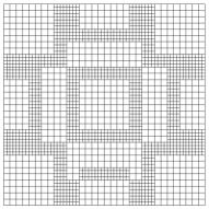
(a) $t=0.00$

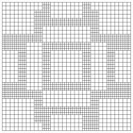
(b) $t=0.25$

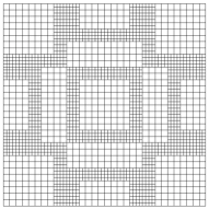
(c) $t=0.75$

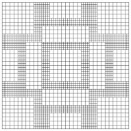
(d) $t=1.00$

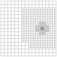
(e) $t=0.00$

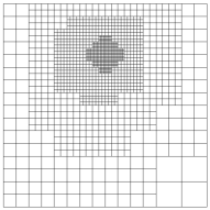
(f) $t=0.25$

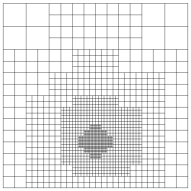
(g) $t=0.75$

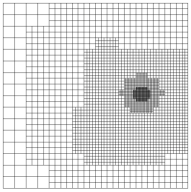
(h) $t=1.00$

Figure 5.2: Comparison of adaptive spatial meshes at selected specific time points for the flow (based on the Kelly Error Estimator) (top, (a)–(d)) and transport (based on the DWR method) (bottom, (e)–(h)) problem, respectively, corresponding to the final loop in Table 5.1.

5.2 Example 2 (Transport in a Constricted Channel)

In this example, we simulate a convection-dominated transport of a species through a channel with a constraint. Here, we investigate the algorithm presented in Sec. 4.3 with regard to fully adaptive space-time refinements of the transport and flow problem obtained by means of the weighted, DWR-based error indicators (4.1) and non-weighted, auxiliary Kelly error indicators (4.2), respectively. The following results may be compared to Example 3 in [13], where a naive, fixed in advance adaptive refinement strategy without using specific error indicators was used for the flow problem. Hence, we study the coupled flow and transport problem with the following setting, where we refer to [13] for further details.

The domain and its boundary colorization are presented by Fig. 5.3, cf. also Rem. 2.1. Precisely, the spatial domain is composed of two unit squares and a constraint in the middle which restricts the channel height by a factor of 5. More precisely, $\Omega=(-1,0)\times(-0.5,0.5)\cup(0,1)\times(-0.1,0.1)\cup(1,2)\times(-0.5,0.5)$ with an initial cell diameter of $h=\sqrt{2\cdot 0.025^{2}}$. The time domain is set to $I=(0,2.5)$. With regard to the characteristic times of the two subproblems defined in (1.3), the coefficients are chosen in such a way that the convective part of $t_{\textnormal{transport}}$ becomes dominant towards the diffusive and reactive part and thus there holds $t_{\textnormal{transport}}\approx t_{\textnormal{flow}}$. Thus, the time domain $I$ is here discretized using the same initial $\sigma=\tau=0.1$ for the flow and transport problem within the first loop $\ell=1$, cf. the first plot in Fig. 5.4. On the left boundary $\Gamma_{\textnormal{in}}$ a time-dependent inflow profile in the positive $x_{1}$-direction is prescribed for the flow field $\mathbf{v}_{D}$ given by

$$\mathbf{v}_{D}(\boldsymbol{x},t)=\begin{cases}\frac{\arctan(t)}{\pi/2}\cdot(1-4x_{2}^{2},0)^{\top}&\textnormal{ for }0\leq t\leq 0.1\,,\\ (1,0)^{\top}&\textnormal{ for }0.1<t\leq T\,.\end{cases}$$ (5.5)

Moreover, for the transport problem, the Dirichlet boundary function value is homogeneous on $\Gamma_{D}$ except for the line $(-1,-1)\times(-0.4,0.4)$ and time $0\leq t\leq 0.1$ where the constant value

$$u(\boldsymbol{x},t)=1$$

is prescribed on the solution. The diffusion coefficient has the constant and small value of $\varepsilon=10^{-4}$ and the reaction coefficient is chosen $\alpha=0.1$. The local SUPG stabilization coefficient is here set to $\delta_{K}=\delta_{0}\cdot h_{K}$, $\delta_{0}=0$, i.e. a vanishing stabilization here. The initial value function $u_{0}=0$ as well as the forcing term $g=0$ are homogeneous. The viscosity is set to $\nu=1$. The goal functional is

$$J(u)=\frac{1}{T\cdot|\Omega|}\displaystyle\int_{I}\int_{\Omega}u(\mathbb{x},t)\,\mathrm{d}\mathbb{x}\mathrm{d}t\,.$$ (5.6)

Finally, the tuning parameters with regard to the adaptive refinement process are chosen here as

$$\begin{array}[]{l@{\,}l@{\,}l@{\,}}\theta_{h,1}^{\textrm{t},\textnormal{top}}\geq\theta_{h,2}^{\textrm{t},\textnormal{top}}=\frac{1}{2}\cdot\min\left\{\frac{|\eta_{h}^{\textrm{t}}|}{|\eta_{h}^{\textrm{t}}|+|\eta_{\tau}^{\textrm{t}}|}\,,1\right\},&\hskip 5.69046pt\theta_{h}^{\textrm{t},\textnormal{bottom}}=0.02\,,&\hskip 5.69046pt\theta_{\tau}^{\textnormal{top}}=\frac{1}{2}\cdot\min\left\{\frac{|\eta_{\tau}^{\textrm{t}}|}{|\eta_{h}^{\textrm{t}}|+|\eta_{\tau}^{\textrm{t}}|}\,,1\right\},\\[6.45831pt] \theta_{h,1}^{\textnormal{{f},top}}=\theta_{h,2}^{\textnormal{{f},top}}=1.0\,,&\hskip 5.69046pt\theta_{h}^{\textnormal{{f},bottom}}=0.0\,,&\hskip 5.69046pt\theta_{\sigma}^{\textnormal{top}}=1.0\textnormal{ (for }0\leq t\leq 0.2)\,,\\[6.45831pt] \varpi=1.0\,,&\hskip 5.69046pt\omega=3.0\,.&\hskip 5.69046pt\theta_{\sigma}^{\textnormal{top}}=0.0\textnormal{ (for }0.2<t\leq 2.5)\,.\end{array}$$

We approximate the primal and dual transport solutions $u$ and $z$ by means of a cG(1)-dG(0) and a cG(2)-dG(0) method, respectively, and the primal flow solution $\mathbf{u}=\{\mathbf{v},p\}$ by means of a {cG(2)-dG(0),cG(1)-dG(0)} discretization.

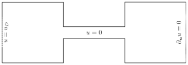
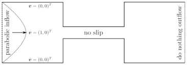
Figure 5.3: Boundary colorization for the transport problem (left) and the coupled flow problem (right) for Sec. 5.2.

In Fig. 5.4, we visualize the distribution of the adaptively determined time cell lengths $\tau_{K}$ and $\sigma_{K}$ used for the transport and flow problem, respectively, over the whole time interval $I$ for different DWR refinement loops. We observe an adaptive refinement in time at the beginning, consistent with the restriction in time of the inflow boundary conditions given above. The closer we get to the final time point $T$ the coarser the temporal mesh is chosen. This behavior nicely brings out the feature of automatically controlled mesh refinement within the underlying algorithm regarding dynamics in time, note that the goal functional (5.6) acts global in time here. These observations are in good agreement to the results obtained for the fixed refinement strategy mentioned above in [13, Ex. 3]. This validates the underlying approach using non-weighted, auxiliary error indicators for the flow problem in order to reduce numerical costs significantly.

Figure 5.4: Distribution of the temporal step size $\tau_{K}$ of the transport problem (based on the DWR method) and $\sigma_{K}$ of the Stokes flow problem (based on the Kelly Error Estimator) over the time interval $I=(0,T]$ for the initial (1) and after 5 and 8 DWR-loops.

5.3 Example 3 (Convection-Dominated Transport with Stabilization)

In a final step, we investigate our multirate approach in view of focusing on the interaction of stabilization techniques combined with goal-oriented error control. For this purpose, we modify Example 2 to the case of a strongly convection-dominated transport problem by increasing the Péclet number by two orders of magnitude. In this case a solely application of adaptive mesh refinement is no longer sufficient to capture strong gradients and avoid spurious and non-physical oscillations. Then, the transport problem additionally has to be stabilized. Here, we compare a non-stabilized solution ($\delta_{0}=0$) with the case of a SUPG stabilized solution ($\delta_{0}\neq 0$) for the transport problem. This final investigation is summarized in the following setting.

We study the coupled flow and transport problem given by (1.1), (1.2) with the same setting as outlined in Example 2., except for the following. The diffusion coefficient has the constant and small value of

$$\varepsilon=10^{-6}\,.$$

The transport problem is stabilized using SUPG stabilization. Therefore, the local SUPG stabilization parameter is set to

$$\delta_{K}=\delta_{0}\cdot h_{K}\,,\delta_{0}=0.1\,.$$

The goal functional is given by (5.6). Finally, the tuning parameters are chosen here as

$$\begin{array}[]{l@{\,}l@{\,}l@{\,}}\theta_{h,1}^{\textrm{t},\textnormal{top}}\geq\theta_{h,2}^{\textrm{t},\textnormal{top}}=\frac{1}{2}\cdot\min\left\{\frac{|\eta_{h}^{\textrm{t}}|}{|\eta_{h}^{\textrm{t}}|+|\eta_{\tau}^{\textrm{t}}|}\,,1\right\},&\hskip 5.69046pt\theta_{h}^{\textrm{t},\textnormal{bottom}}=0.02\,,&\hskip 5.69046pt\theta_{\tau}^{\textnormal{top}}=\frac{1}{2}\cdot\min\left\{\frac{|\eta_{\tau}^{\textrm{t}}|}{|\eta_{h}^{\textrm{t}}|+|\eta_{\tau}^{\textrm{t}}|}\,,1\right\},\\[6.45831pt] \theta_{h,1}^{\textnormal{{f},top}}=\theta_{h,2}^{\textnormal{{f},top}}=0.33\,,&\hskip 5.69046pt\theta_{h}^{\textnormal{{f},bottom}}=0.02\,,&\hskip 5.69046pt\theta_{\sigma}^{\textnormal{top}}=0.2\,,\\[6.45831pt] \varpi=1.0\,,&\hskip 5.69046pt\omega=3.0\,.&\end{array}$$

We approximate the primal and dual transport solution $u$ and $z$ by means of a cG(1)-dG(0) and cG(2)-dG(0) method, respectively, on adaptively refined meshes in space and time based on weighted error indicators based on the DWR method, given by Eq. (4.1). However, the flow solution $\mathbf{u}=\{\mathbf{v},p\}$ is approximated with a {cG(2)-dG(0),cG(1)-dG(0)} discretization on adaptively refined meshes in space and time based on auxiliary, non-weighted error indicators based on the Kelly Error Estimator, given by Eq. (4.2).

In Fig. 5.5, we compare the solution profiles and corresponding adaptive spatial meshes of the primal transport solution $u_{\tau h}^{1,0}$ for a non-stabilized and stabilized case, respectively, at selected time points within the final DWR loop $\ell=8$. It becomes clear that in the strongly convection-dominated case a solely adaptive mesh refinement without stabilization is no longer sufficient to resolve the arising layers of the transported species within the channel, especially regarding the solution profiles in the course of time; cf. the blurred solution profiles in the course of the transported species on the left part of Fig. 5.5. This becomes even clearer considering the exemplary side profile of the primal transport solution at time $t=1.35$ given by the upper part of Fig. 5.6 that is strongly perturbed by means of spurious and non-physical oscillations, especially in the part of the constriction within the channel. Without additional stabilization techniques the underlying algorithm is not able to capture the strong gradients and resolve the layers and sharp moving fronts of the underlying transported species. In contrast, regarding the stabilized solution profiles given by the right and lower part of Fig. 5.5 and Fig. 5.6, respectively, the solution profile fronts are resolved in a visibly more accurate way along with a significantly reduction of the spurious oscillations. Moreover, regarding the underlying spatial meshes, we point out that in the stabilized case the adaptive refinement is located close to the whole solution front of the underlying transported species within the channel. More precisely, we observe local refinements located in the left unit square corresponding to the wing-like fronts and behind them, within the constriction corresponding to the course of the solution profile as well as at the exit of the restriction, in particular at the corners of the exit, corresponding to the head of the solution profile.

In contrast to that, in the non-stabilized case most of the local refinement takes place at the beginning of the constriction where most of the oscillations are visible. In comparison, the remaining parts along the solution front are less refined, in particular, regarding the wing-like fronts in the left unit square. This is obvious since the goal functional (5.6) acts global in space and time and thus those parts of the error indicators are weighted stronger involving larger errors in the respective quantity.

Due to the additional stabilization along with a significantly reduction of the oscillations, the algorithm in the stabilized case is capable to distribute the refinement more evenly to the regions belonging to strong gradients of the underlying solution profile. In summary, the stabilized solution shows a significantly improvement with regard to resolving layers and sharp moving fronts along with efficient underlying spatial meshes, even though some slight perturbations located at the course of the layers are still visibly.

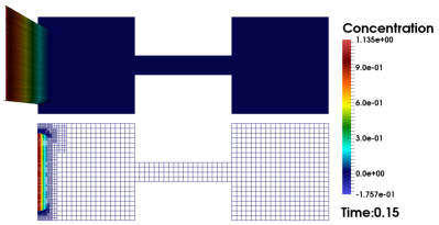
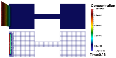
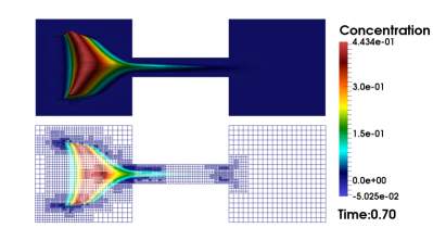
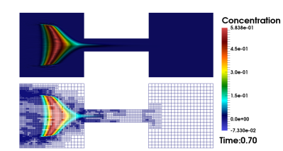
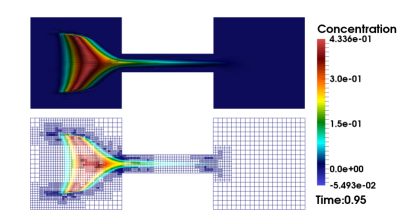
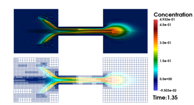
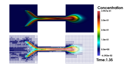
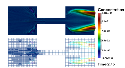
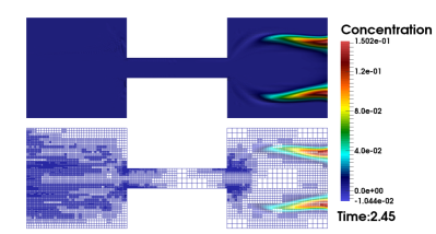
Figure 5.5: Comparison of transport solution profiles and related adaptively refined spatial meshes (based on the DWR method) without stabilization $\delta_{0}=0.0$ (left) and with SUPG stabilization $\delta_{0}=0.1$ (right) for $\varepsilon=10^{-6}$ at different time points corresponding to loop $\ell=8$ for Example 3.

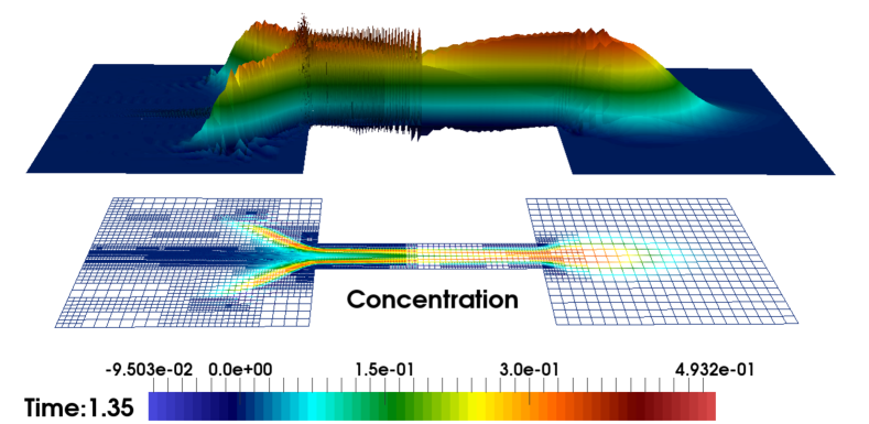
(a) No Stabilization ($\delta_{0}=0.0$), 29843 spatial DoFs

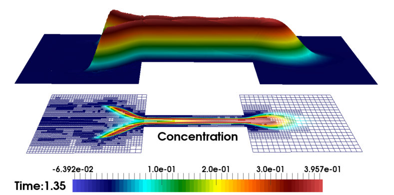
(b) SUPG Stabilization ($\delta_{0}=0.1$), 27471 spatial DoFs

Figure 5.6: Comparison of side profiles for the transport solution and related adaptively refined spatial meshes (based on the DWR method) without stabilization $\delta_{0}=0.0$ (top) and with SUPG stabilization $\delta_{0}=0.1$ (bottom) for $\varepsilon=10^{-6}$ corresponding to loop $\ell=8$ for Example 3, exemplary at time point $t=1.35$.

Finally, for the sake of completeness, we present in Fig. 5.7 the solution profile and corresponding adaptive spatial mesh of the primal flow field solution $\mathbf{v}_{\sigma h}$ based on the Kelly Error Estimator, exemplary at time $t=0.1$ corresponding to the time-dependence of the inflow boundary condition given by (5.5) within the final loop $\ell=8$. The adaptive spatial refinement is located to the spreading of the convection flow field $\mathbf{v}_{\sigma h}$, cf. the upper plot of Fig. 5.7. Moreover, the spatial mesh is visibly more refined close to the corners of the entrance and exit of the channels’ constriction consistent with occurring challenges arising in such regions of the underlying meshes, cf., e.g., [35, 18].

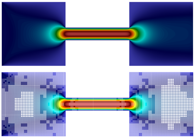
Figure 5.7: Convection $\mathbf{v}_{\sigma h}$ solution of the Stokes flow problem and related adaptively refined spatial mesh (based on the Kelly Error Estimator) with $Q_{2}$-$Q_{1}$ finite elements and 48186 spatial DoFs, corresponding to loop $\ell=8$ for Example 3, exemplary at time point $t=0.1$. On the left boundary a time-dependent inflow profile in the positive $x_{1}$-direction is prescribed for the convection $\mathbf{v}_{D}$ given by Eq. (5.5).

6 Summary

In this work, we presented a cost-efficient space-time adaptive algorithm for our multirate approach combined with stabilization and goal-oriented error control based on the DWR method applied to coupled flow and transport. Different adaptive time step sizes on different temporal meshes initialized with the help of characteristic times were used for the two subproblems. Furthermore, the transport problem was assumed to be convection-dominated and thus stabilized using the residual based SUPG method which puts an additional facet of complexity on the algorithmic design. Both subproblems are discretized using a discontinuous Galerkin method dG($r$) with an arbitrary polynomial degree $r\geq 0$ in time and a continuous Galerkin method cG($p$) with an arbitrary polynomial degree $p\geq 1$ in space. Goal-oriented a posteriori error representation based on the DWR method were derived for the flow as well as for transport problem. These error representations are splitted into quantities in space and time such that their localized forms serve as error indicators for the adaptive mesh refinement process in space and time. To reduce numerical costs significantly, in the numerical experiments such weighted error indicators were used only within the adaptivity for the transport problem, where the adaptivity for the flow problem was achieved by using auxiliary, non-weighted error indicators based on the Kelly Error Estimator that avoids an explicit computation of a dual flow problem. Nevertheless, considering duality for the flow problem within the numerical examples is work that remains to be done and will be interesting to be compared to the results obtained in the present work.

The practical realization as well as some implementational aspects regarding the specifications within the multirate approach were demonstrated. In numerical experiments, the algorithm was studied with regard to accuracy, efficiency and reliability reasons by investigating a typical benchmark as well as a problem of practical interest. Spurious oscillations that typically arise in numerical approximations of convection-dominated problems could be reduced significantly. High-efficient adaptively refined meshes in space and time were obtained for both subproblems, where using auxiliary, non-weighted error indicators for the flow problem had any negative impact on the adaptive refinement process for the transport problem as effectivity indices close to one and well-balanced error indicators in space and time were obtained. Moreover, the numerical results give a first hint of the potential regarding a temporal mesh that is adapted to the dynamics of the active or fast components compared to a more standard fixed-time strategy where the whole mesh is refined due to these fast components. Finally, the here presented approach for coupled flow and transport is fairly general and can be easily adopted to other multi-physics systems coupling phenomena that are characterized by strongly differing time scales.

Appendix

In the Appendix, we give some detailed definitions and remarks regarding the main results derived in Se. 3.

Galerkin Orthogonality for Temporal and Spatial Error of Transport Problem

For the temporal error $e={u}-{u}_{\tau}$ we get the following Galerkin orthogonality by subtracting Eq. (2.10) from Eq. (2.5)

$$\begin{array}[]{l}\displaystyle\sum_{n=1}^{N^{\ell}}\sum_{K_{n}\in\mathcal{T}_{\tau,n}}\int_{K_{n}}\big{\{}(\partial_{t}e,\varphi_{\tau})+a(e,\mathbf{v}_{\sigma})(\varphi_{\tau})\big{\}}\mathrm{d}t\\[6.45831pt] =\displaystyle\sum_{t_{F}\in\mathcal{F}_{\tau}}([u_{\tau}]_{t_{F}},\varphi_{\tau}(t_{F}^{+}))\displaystyle-\sum_{n=1}^{N^{\ell}}\sum_{K_{n}\in\mathcal{T}_{\tau,n}}\int_{K_{n}}\big{(}(\mathbf{v}-\mathbf{v}_{\sigma})\cdot\nabla{u},\varphi_{\tau}\big{)}\mathrm{d}t\,,\end{array}$$ (6.1)

with a non-vanishing right-hand side term depending on the the temporal error in the approximation of the flow field. For the spatial error $e={u}_{\tau}-{u}_{\tau h}$ we get the following Galerkin orthogonality by subtracting Eq. (2.14) from Eq. (2.10)

$$\begin{array}[]{l}\displaystyle\sum_{n=1}^{N^{\ell}}\sum_{K_{n}\in\mathcal{T}_{\tau,n}}\int_{K_{n}}\big{\{}(\partial_{t}e,\varphi_{\tau h})+a(e;\mathbf{v}_{\sigma h})(\varphi_{\tau h})\big{\}}\mathrm{d}t\\ +\displaystyle\sum_{t_{F}\in\mathcal{F}_{\tau}}([e]_{t_{F}},\varphi_{\tau h}(t_{F}^{+})+(e(0^{+}),\varphi_{\tau h}(0^{+}))\\ =\displaystyle S_{A}({u}_{\tau h};\mathbf{v}_{\sigma h})(\varphi_{\tau h})-\sum_{n=1}^{N^{\ell}}\sum_{K_{n}\in\mathcal{T}_{\tau,n}}\int_{K_{n}}\big{(}(\mathbf{v}_{\sigma}-\mathbf{v}_{\sigma h})\cdot\nabla{u}_{\tau},\varphi_{\tau h}\big{)}\mathrm{d}t\,,\end{array}$$ (6.2)

with a non-vanishing right-hand side term depending on the stabilization and the spatial error in the approximation of the flow field.

Transport: Dual Problems and Residuals

Within the context of the DWR philosophy, the dual problems are generally given as optimality or stationary conditions regarding the underlying Lagrangian functionals. More precisely, considering the directional derivatives of the Lagrangian functionals (3.3), also known as Gâteaux derivatives (cf., e.g., [9]), with respect to their first argument, i.e.

$$\mathcal{L}^{\prime}_{{u}}({u},{z};\mathbf{v})(\varphi):=\lim_{t\neq 0,t\rightarrow 0}t^{-1}\big{\{}\mathcal{L}({u}+t\varphi,{z};\mathbf{v})-\mathcal{L}({u},{z};\mathbf{v})\big{\}},\quad\varphi\in\mathcal{X}\,,$$

leads to the following dual transport problems: Find the continuous dual solution ${z}\in\mathcal{X}$, the semi-discrete dual solution ${z}_{\tau}\in\mathcal{X}_{\tau}^{r}$ and the fully discrete dual solution ${z}_{\tau h}\in\mathcal{X}_{\tau h}^{r,p}$, respectively, such that

$$\begin{array}[]{r@{\,}c@{\,}l@{\,}l@{\,}}A^{\prime}({u};\mathbf{v})(\varphi,{z})&=&J^{\prime}({u})(\varphi)&\quad\forall\varphi\in\mathcal{X}\,,\\[4.30554pt] A_{\tau}^{\prime}({u}_{\tau};\mathbf{v}_{\sigma})(\varphi_{\tau},{z}_{\tau})&=&J^{\prime}({u}_{\tau})(\varphi_{\tau})&\quad\forall\varphi_{\tau}\in\mathcal{X}_{\tau}^{r}\,,\\[4.30554pt] A_{S}^{\prime}({u}_{\tau h};\mathbf{v}_{\sigma h})(\varphi_{\tau h},{z}_{\tau h})&=&J^{\prime}({u}_{\tau h})(\varphi_{\tau h})&\quad\forall\varphi_{\tau h}\in\mathcal{X}_{\tau h}^{r,p}\,,\end{array}$$ (6.3)

where we refer to our works [7, 12] for a detailed description of the adjoint bilinear forms $A^{\prime},A_{\tau}^{\prime},A_{S}^{\prime}$ as well as the dual right hand side term $J^{\prime}$.

The primal and dual residuals based on the continuous and semi-discrete in time schemes are defined by means of the Gâteaux derivatives of the Lagrangian functionals in the following way:

$$\begin{array}[]{r@{\;}c@{\;}l@{\;}c@{\;}l@{\;}}\rho(u;\mathbf{v})(\varphi)&:=&\mathcal{L}_{{z}}^{\prime}({u},{z};\mathbf{v})(\varphi)&=&G(\varphi)-A({u};\mathbf{v})(\varphi)\,,\\[6.45831pt] \rho^{\ast}({u},{z};\mathbf{v})(\varphi)&:=&\mathcal{L}_{{u}}^{\prime}({u},{z};\mathbf{v})(\varphi)&=&J^{\prime}({u})(\varphi)-A^{\prime}({u};\mathbf{v})(\varphi,{z})\,,\\[6.45831pt] \rho_{\tau}({u};\mathbf{v}_{\sigma})(\varphi)&:=&\mathcal{L}_{\tau,{z}}^{\prime}({u},{z};\mathbf{v}_{\sigma})(\varphi)&=&G_{\tau}(\varphi)-A_{\tau}({u};\mathbf{v}_{\sigma})(\varphi)\,,\\[6.45831pt] \rho_{\tau}^{\ast}({u},{z};\mathbf{v}_{\sigma})(\varphi)&:=&\mathcal{L}_{\tau,{u}}^{\prime}({u},{z};\mathbf{v}_{\sigma})(\varphi)&=&J^{\prime}({u})(\varphi)-A_{\tau}^{\prime}({u};\mathbf{v}_{\sigma})(\varphi,{z})\,.\end{array}$$

Flow: Dual Problems and Residuals

For the sake of completeness, considering the directional derivatives of the Lagrangian functionals (3.1), also known as Gâteaux derivatives (cf., e.g., [9]), with respect to their first argument, i.e.

$$\mathcal{L}^{\prime}_{\mathbf{u}}(\mathbf{u},\mathbf{z})(\boldsymbol{\varphi}):=\lim_{t\neq 0,t\rightarrow 0}t^{-1}\big{\{}\mathcal{L}(\mathbf{u}+t\boldsymbol{\varphi},\mathbf{z})-\mathcal{L}(\mathbf{u},\mathbf{z})\big{\}},\quad\boldsymbol{\varphi}\in\mathcal{Y}\,,$$

leads to the following dual flow problems, although these problems were not used within the underlying cost reduced approach here: Find the continuous dual flow solution $\mathbf{z}=\{\mathbf{w},q\}\in\mathcal{Y}$, the semi-discrete dual flow solution $\mathbf{z}_{\sigma}=\{\mathbf{w}_{\sigma},q_{\sigma}\}\in\mathcal{Y}_{\sigma}^{r}$ and the fully discrete dual flow solution $\mathbf{z}_{\sigma h}\{\mathbf{w}_{\sigma h},q_{\sigma h}\}\in\mathcal{Y}_{\sigma h}^{r,p}$, respectively, such that

$$\begin{array}[]{r@{\,}c@{\,}l@{\,}l@{\,}}B^{\prime}(\mathbf{u})(\boldsymbol{\varphi},\mathbf{z})&=&J^{\prime}(\mathbf{u})(\boldsymbol{\varphi})&\quad\forall\boldsymbol{\varphi}=\{\boldsymbol{\psi},\chi\}\in\mathcal{Y}\,,\\[4.30554pt] B_{\sigma}^{\prime}(\mathbf{u}_{\sigma})(\boldsymbol{\varphi}_{\sigma},\mathbf{z}_{\sigma})&=&J^{\prime}(\mathbf{u}_{\sigma})(\boldsymbol{\varphi}_{\sigma})&\quad\forall\boldsymbol{\varphi}_{\sigma}=\{\boldsymbol{\psi}_{\sigma},\chi_{\sigma}\}\in\mathcal{Y}_{\sigma}^{r}\,,\\[4.30554pt] B_{\sigma h}^{\prime}(\mathbf{u}_{\sigma h})(\boldsymbol{\varphi}_{\sigma h},\mathbf{z}_{\sigma h})&=&J^{\prime}(\mathbf{u}_{\sigma h})(\boldsymbol{\varphi}_{\sigma h})&\quad\forall\boldsymbol{\varphi}_{\sigma h}=\{\boldsymbol{\psi}_{\sigma h},\chi_{\sigma h}\}\in\mathcal{Y}_{\sigma h}^{r,p}\,,\end{array}$$ (6.4)

where we refer to [12] for a detailed description of the adjoint bilinear forms $B^{\prime},B_{\sigma}^{\prime},B_{\sigma h}^{\prime}$ as well as the dual right hand side term $J^{\prime}$.

Finally, the primal and dual residuals based on the semi-discrete in time schemes are defined by means of the Gâteaux derivatives of the Lagrangian functionals in the following way:

$$\begin{array}[]{r@{\;}c@{\;}l@{\;}c@{\;}l@{\;}}\rho_{\sigma}(\mathbf{u})(\boldsymbol{\varphi})&:=&\mathcal{L}_{\sigma,\mathbf{z}}^{\prime}(\mathbf{u},\mathbf{z})(\boldsymbol{\varphi})&=&F_{\sigma}(\boldsymbol{\psi})-B_{\sigma}(\mathbf{u})(\boldsymbol{\varphi})\,,\\[6.45831pt] \rho_{\sigma}^{\ast}(\mathbf{u},\mathbf{z})(\boldsymbol{\varphi})&:=&\mathcal{L}_{\sigma,\mathbf{u}}^{\prime}(\mathbf{u},\mathbf{z})(\boldsymbol{\varphi})&=&J^{\prime}(\mathbf{u})(\boldsymbol{\varphi})-B_{\sigma}^{\prime}(\mathbf{u})(\boldsymbol{\varphi},\mathbf{z})\,.\end{array}$$

References

• [1] E. Ahmed, Ø. Klemetsdal, X. Raynaud, O. Møyner and H. M. Nilsen, Adaptive Timestepping, Linearization, and A Posteriori Error Control for Multiphase Flow of Immiscible Fluids in Porous Media with Wells, SPE Journal (2022), 1–21.
• [2] T. Almani and K. Kumar, Convergence of single rate and multirate undrained split iterative schemes for a fractured biot model, Comput. Geosci. 26 (2022), 975–994.
• [3] T. Almani, K. Kumar, G. Singh and M.F. Wheeler, Stability of multirate explicit coupling of geomechanics with flow in a poroelastic medium, Comput. Math. Appl. 78(7) (2019), 2682–2699.
• [4] D. Arndt, W. Bangerth, B. Blais, M. Fehling, R. Gassmöller, T. Heister, L. Heltai, U. Köcher, M. Kronbichler, M. Maier, P. Munch, J.-P. Pelteret, S. Proell, K. Simon, B. Turcksin, D. Wells and J. Zhang, The deal.II Library, Version 9.3. J. Numer. Math. 29(3) (2021), 171–186.
• [5] D. Avijit and S. Natesan, An efficient DWR-type a posteriori error bound of SDFEM for singularly perturbed convection-diffusion PDEs, J. Sci. Comput. 90(73) (2022).
• [6] W. Bangerth and R. Rannacher, Adaptive finite element methods for differential equations, Birkhäuser, Basel, 2003.
• [7] M. Bause, M. P. Bruchhäuser and U. Köcher, Flexible goal-oriented adaptivity for higher-order space-time discretizations of transport problems with coupled flow, Comput. Math. Appl. 91 (2021), 17–35.
• [8] R. Becker and R. Rannacher, An optimal control approach to a posteriori error estimation in finite element methods, in: Iserles, A. (Ed.) Acta Numer., Vol. 10, Cambridge University Press (2001), 1–102.
• [9] M. Besier and R. Rannacher, Goal-oriented space-time adaptivity in the finite element galerkin method for the computation of nonstationary incompressible flow, Int. J. Num. Methods Fluids 70(9) (2012), 1139–1166.
• [10] A. Brenner, E. Bänsch and M. Bause, A-priori error analysis for finite element approximations of Stokes problem on dynamic meshes, IMA J. Numer. Anal. 34 (2014), 123–146.
• [11] A. N. Brooks and T. J. R. Hughes, Streamline upwind/Petrov-Galerkin formulations for convection dominated flows with particular emphasis on the incompressible Navier-Stokes equations, Comput. Methods Appl. Mech. Engrg. 32(1-3) (1982), 199–259.
• [12] M. P. Bruchhäuser, Goal-oriented space-time adaptivity for a multirate approach to coupled flow and transport, Ph.D. thesis, Helmut-Schmidt-University / University of the Federal Armed Forces Hamburg, 2022.
• [13] M. P. Bruchhäuser, U. Köcher and M. Bause, On the implementation of an adaptive multirate framework for coupled transport and flow, J. Sci. Comput. 93 59 (2022), DOI: 10.1007/s10915-022-02026-z.
• [14] E. Burman, Robust error estimates in weak norms for advection dominated transport problems with rough data. Math. Models Methods Appl. Sci. 24(13) (2014), 2663–2684.
• [15] G. F. Carey and J. T. Oden, Finite Elements, Computational Aspects, Vol. III (The Texas finite element series), Prentice-Hall, Englewood Cliffs, New Jersey, 1984.
• [16] Z. Ge and M. Ma, Multirate iterative scheme based on mutiphysics discontinuous Galerkin method for a poroelasticity model. Appl. Numer. Math. 128 (2018), 125–138.
• [17] S. Gupta, B. Wohlmuth and R. Helmig, Multirate time stepping schemes for hydro-geomechanical model for subsurface methane hydrate reservoirs, Adv. Water Res. 91 (2016), 78–87.
• [18] B. Endtmayer and T. Wick, A partition-of-unity dual-weighted residual approach for multi-objective goal functional error estimation applied to elliptic problems, Comput. Methods Appl. Math. 17(4) (2017), 575-599.
• [19] B. Endtmayer, U. Langer and T. Wick, Reliability and Efficiency of DWR-Type A Posteriori Error Estimates with Smart Sensitivity Weight Recovering, Comput. Methods Appl. Math. 21(2) (2021), 351–371.
• [20] A. Ern and J.-L. Guermond, Finite elements III: First-order and time-dependent pdes, Texts in Applied Mathematics, Vol. 74, Springer, Cham, 2021.
• [21] M. J. Gander and L. Halpern, Techniques for locally adaptive time stepping developed over the last two decades, in: Bank, R., Holst, M., Widlund, O., Xu, J. (Eds.), Domain Decomposition Methods in Science and Engineering XX, Lecture Notes in Computational Science and Engineering 91, Springer, Berlin, Heidelberg (2013), 377–385
• [22] W. Gujer, Systems Analysis for Water Technology, Springer, Berlin, Heidelberg, 2008.
• [23] R. Hartmann, A-posteriori Fehlerschätzung und adaptive Schrittweiten- und Ortsgittersteuerung bei Galerkin-Verfahren für die Wärmeleitungsgleichung, Diploma Thesis, Institute of Applied Mathematics, University of Heidelberg, 1998.
• [24] T. J. R. Hughes and A. N. Brooks, A multidimensional upwind scheme with no crosswind diffusion. in: Finite Element Methods for Convection Dominated Flows, AMD, Vol. 34, Amer. Soc. Mech. Engrs. (ASME) (1979), 19–35.
• [25] M. Jammoul, M. F. Wheeler and T. Wick, A phase-field multirate scheme with stabilized iterative coupling for pressure driven fracture propagation in porous media, Comput. Math. Appl. 91 (2021), 176–191.
• [26] V. John, Finite element methods for incompressible flow problems Springer Series in Computational Mathematics, Vol.51, Springer, Cham, 2016.
• [27] V. John and E. Schmeyer, Finite element methods for time-dependent convection-diffusion-reaction equations with small diffusion, Comput. Methods Appl. Mech. Engrg. 198 (2009), 173–181.
• [28] V. John, P. Knobloch and J. Novo, Finite elements for scalar convection-dominated equations and incompressible flow problems: a never ending story? Comput. Vis. Sci. 19 (2018), 47–63.
• [29] D.W. Kelly, S. R. De, J. P. Gago, O. C. Zienkiewicz and I. Babuska, A posteriori error analysis and adaptive processes in the finite element method: Part I—error analysis. Int. J. Numer. Meth. Engng. 19 (1983), 1593-1619. https://doi.org/10.1002/nme.1620191103
• [30] U. Köcher, M. P. Bruchhäuser and M. Bause, Efficient and scalable data structures and algorithms for goal-oriented adaptivity of space–time FEM codes, Software X, 10:100239 (2019).
• [31] M. G. Larson, A. Mlquist, Goal oriented adaptivity for coupled flow and transport with applications in oil reservoir simulations, Comput. Methods Appl. Mech. Engrg 196 (2007), 3546–3561.
• [32] E. Morgenroth, How are characteristic times ($\tau_{\textrm{char}}$) and non-dimensional numbers related.
https://ethz.ch/content/dam/ethz/special-interest/baug/ifu/water-management-dam/documents/education/Lectures/UWM3/SAMM.HS15.Handout.CharacteristicTimes.pdf (2015). Accessed 07 February 2022
• [33] H.-G. Roos, M. Stynes and L. Tobiska, Robust Numerical Methods for Singularly Perturbed Differential Equations, Springer, Berlin, 2008.
• [34] M. Schmich, Adaptive finite element methods for computing nonstationary incompressible flows, Ph.D. thesis, University of Heidelberg, 2009.
• [35] M. Schmich and B. Vexler, Adaptivity with dynamic meshes for space-time finite element discretizations of parabolic equations, SIAM J. Sci. Comput. 30(1) (2008), 369–393.
• [36] M. Soszyńska and T. Richter, Adaptive time-step control for a monolithic multirate scheme coupling the heat and wave equation, BIT Numer. Math. 61 (2021), 1367–1396.