Safe Imitation Learning of Nonlinear Model Predictive Control
for Flexible Robots

Abstract

Flexible robots may overcome some of the industry’s major challenges, such as enabling intrinsically safe human-robot collaboration and achieving a higher load-to-mass ratio. However, controlling flexible robots is complicated due to their complex dynamics, which include oscillatory behavior and a high-dimensional state space. Nonlinear model predictive control (NMPC) offers an effective means to control such robots, but its extensive computational demands often limit its application in real-time scenarios. To enable fast control of flexible robots, we propose a framework for a safe approximation of NMPC using imitation learning and a predictive safety filter. Our framework significantly reduces computation time while incurring a slight loss in performance. Compared to NMPC, our framework shows more than a eightfold improvement in computation time when controlling a three-dimensional flexible robot arm in simulation, all while guaranteeing safety constraints. Notably, our approach outperforms conventional reinforcement learning methods. The development of fast and safe approximate NMPC holds the potential to accelerate the adoption of flexible robots in industry.

I INTRODUCTION

In recent years flexible robots have been drawing more attention as they might hold the key to the industry’s significant problems. These problems include increasing the load-to-mass ratio and making robots intrinsically safer to facilitate human-robot collaboration. The main reason why flexible robots have yet to be adopted is the flexibility that causes oscillations and static deflections, complicating modeling and control.

Modeling flexible robots is challenging as they have an infinite number of degree of freedom (DOF) and are governed by nonlinear partial differential equations (PDE). Discretization converts PDE into ordinary differential equations (ODE), making them suitable for control and trajectory planning. There are three main methods for discretizing a flexible link: the assumed mode method (AMM) [1, 2], the finite element method (FEM) [3, 4] and the lumped parameter method (LPM) [5, 6, 7, 8]. All the methods generally assume small deformations and use the linear theory of elasticity. The FEM is the most accurate among the three but results in a higher number of differential equations. The AMM is often used for one DOF flexible robots; for robots with higher DOF, the choice of boundary conditions becomes nontrivial [9]. The LPM is the simplest among all, but tuning the parameters of such models takes much work. In this paper, we leverage the LPM following a formulation defined in [10], where the method is called the modified rigid FEM (MRFEM). Section III describes the method in detail.

Many control methods have been proposed for controlling flexible robots, including optimal control methods. Green et al. [2] applied LQR for trajectory tracking control of a two-link flexible robot using linearized dynamics. [11] and [12] used MPC to control a single-link flexible robot and four-link flexible mechanisms, respectively. In both cases, the authors linearized the dynamics and used linear MPC, highlighting the challenge of designing fast NMPC for robots with the high dimensional dynamics.

To make NMPC available for a broader range of systems, recently there have been attempts to approximate NMPC with neural networks (NN) [13]. [14] proposed using supervised learning to approximate robust NMPC, while [15] proposed a policy search method guided by NMPC without safety considerations. To ensure that the approximate NMPC provides safe inputs (that does not violate constraints), [14] leveraged a statistical validation technique to obtain safety guarantees. The authors reported that the validation process is time-consuming. In general, approximating NMPC with NN fits under the umbrella of imitation learning (IL). [16] discusses various methods for ensuring the safety of learning methods. One particular approach to guarantee the safety of a learned policy is the safety filter (SF) [17]: an NMPC scheme that receives a candidate input and verifies if it can drive the system to a safe terminal set after applying the candidate input. If the answer is positive, the input is applied to the system; otherwise, it is modified as little as possible to ensure safety. [18] successfully used SF for a multi-agent drone setup that was trained with reinforcement learning (RL). To the best of the authors knowledge, this paper is the first that investigates whether IL combined with SF can replace NMPC for safe regulation control of flexible robots. We show that our particular implementation successfully lowers computation time of the controller, filters unsafe controls while operating close to the expert’s performance.

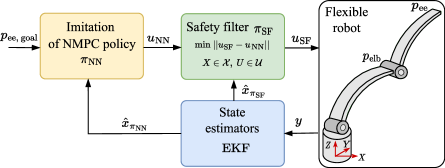
Figure 1: Pipeline for safely approximating NMPC policy by combining imitation learning and a safety filter.

In particular our contributions are: (i) efficient NMPC formulation for controlling flexible robots; (ii) a framework for safely approximating NMPC for flexible robots; (iii) simulation experiments with a baseline RL algorithms.

The paper is organized as follows: Section II outlines the proposed framework, Section III describes the setup, Section IV-A details NMPC and safety filter formulations, as well as training of IL methods. Section V presents simulation experiments and discusses the results. Finally, in Section VI, we make concluding remarks.

II SAFE APPROXIMATE NMPC

Let $\bm{x}\in\mathbb{R}^{n_{x}}$, $\bm{u}\in\mathbb{R}^{n_{u}}$ and $\bm{z}\in\mathbb{R}^{n_{z}}$ denote the state, control inputs, and controlled output of a flexible robot. Furthermore, let the dynamics be defined in state-space form as

$$\dot{\bm{x}}=\bm{f}(\bm{x},\bm{u});\quad\bm{z}=\bm{h}(\bm{x}).$$ (1)

Our focus lies in addressing the output regulation problem: steering a robot from an initial rest state $\bm{x}_{0}$ to a goal state $\bm{x}^{\mathrm{ref}}$ that corresponds to the output $\bm{z}^{\mathrm{ref}}=\bm{h}(\bm{x}^{\mathrm{ref}})$. Additionally, the controller must respect the constraints of the robot such as velocity and input/torque constraints as well as avoid obstacles. This task can be solved by an NMPC which maps the current state into a control action which we denote as $\bm{\pi}_{\text{NMPC}}(\bm{x})$. However, flexible robots with high dimensional state-space and highly nonlinear dynamics, pose substantial challenges to executing NMPC in real-time. This leads to the main question of our paper:

How can we approximate the NMPC policy $\bm{\pi}_{\text{NMPC}}(\bm{{x}})$ for controlling flexible robots that simultaneously reduces the computational burden and ensures safety?

In pursuit of a solution, we propose a framework, as illustrated in Fig. 1, that aims to achieve both objectives. The approach involves two steps. Initially, it approximates $\bm{\pi}_{\text{NMPC}}({\bm{x}})$ using a NN through imitation learning, thereby yielding $\bm{\pi}_{\mathrm{NN}}(\bm{{x}})$. Subsequently, during operational runtime, our approach filters the output of the learned policy $\bm{u}_{\text{NN}}$ using a safety filter $\bm{\pi}_{\text{SF}}(\bm{u})$, which either accepts or modifies $\bm{u}_{\text{NN}}$ based on predefined safety criteria. The following subsections describe the fundamental components of the framework.

II-A Nonlinear model predictive control

NMPC is a model-based method that leverages nonlinear optimization solvers to determine a sequence of control actions for achieving a specific task, such as regulation. Typically, NMPC is initially formulated in continuous time, after which it is discretized and represented as a nonlinear program (NLP) [19]. Various techniques are available for translating NMPC into an NLP, and this paper adopts the direct multiple shooting approach [20], where the decision variables are both states and control actions. A general NLP for regulating a flexible robot can be expressed as follows: [3] X, U ∑_i=0^N-1∥h(x_i)- z^ref ∥^2_Q + ∥u_i -u^ref ∥^2_R +V(x_N) 0=Φ(x_k+1, x_k, u_k),k=0,…,N-1 0≤h(x_k),k=0,…,N x_0=¯x,  u_k ∈U,k=0,…,N-1 x_k ∈X,k=0,…,N x_N ∈X^S. In this formulation, $N$ represents the prediction horizon, $\bm{X}=[\bm{x}_{0},\ldots,\bm{x}_{N}]\in\mathbb{R}^{n_{x}\times(N+1)}$ and $\bm{U}=[\bm{u}_{0},\ldots,\bm{u}_{N-1}]\in\mathbb{R}^{n_{u}\times N}$ are the decision variables for the state and control, respectively. Additionally, $\mathcal{X}\subseteq\mathbb{R}^{n_{x}}$ and $\mathcal{U}\subseteq\mathbb{R}^{n_{u}}$ define the feasible state and control sets. The cost function (2a) penalizes deviations from the desired output and control actions, employing squared weighted $L^{2}$ norms with the weighting matrices $\bm{Q}$ and $\bm{R}$, respectively. Furthermore, the cost function incorporates a terminal cost, $V(\bm{x}_{N})$, which approximates the cost from $N$ to infinity.

The constraints consist of the discretized nonlinear dynamics of the robot (II-A), path constraints like obstacle and self-collision avoidance (II-A), and control and state constraints as given in equations (II-A) and (II-A), respectively. Finally, a positive invariant safe set $\mathcal{X}^{\mathrm{s}}\subseteq\mathbb{R}^{n_{x}}$ is often used to obtain recursive feasibility. NMPC solves a parametric NLP iteratively based on the current state $\bar{\bm{x}}$ and utilizes a dedicated solver, such as [21], to compute the optimal solution. Subsequently, the first control input $\bm{u}_{0}$ is applied to the system

II-B Imitation learning

The aim of IL is to approximate the NMPC policy $\pi_{\text{NMPC}}$ (II-A), also referred as the expert policy, by a NN using a dataset of expert demonstrations $\mathcal{D}=\{(\bm{u}_{\mathrm{NMPC},i},\bm{x_{i}},\bm{s}_{i})\}_{i=1}^{N}$, where $\bm{s}$ represents relevant environmental parameters, such as obstacle representation. Behavioral Cloning (BC) [22] is a simple IL method that approximates the expert policy by solving a supervised regression problem on $\mathcal{D}$. However, BC is limited as it can occasionally make mistakes, causing it to venture into areas of the state space not covered in $\mathcal{D}$. This results in unpredictable behavior and poor performance. The DAgger algorithm [23] addresses the limitations of BC. It collects additional expert demonstrations $\mathcal{D}_{\mathrm{new}}$ while the robot interacts with the environment under the state distribution induced by the learned policy. In other words, DAgger learns from the expert to correct for the approximation errors accumulated by the learned policy.

In contrast to IL and DAgger, there exists a family of methods known as Inverse Reinforcement Learning (IRL). These methods aim to learn the reward function $r$ of the expert from the dataset $\mathcal{D}$ and train a policy based on this learned reward function $r$. Although IRL methods can lead to more robust policies, they are often challenging to train due to their adversarial nature. In the Section V, we train and compare several IL methods designed to approximate the expert policy $\bm{\pi}_{\text{NMPC}}(\bm{x})$ for regulating flexible robots.

II-C Safety filter

The safety filter [17], when applied, ensures the safety of learned policies and is formulated in a manner nearly equivalent to (II-A) but much cheaper computationally. However, it employs a simpler model, potentially with a lower-dimensional state space, and has a cost

$$\tilde{L}_{\mathrm{SF}}(\bm{u}_{0})=\left\lVert\bm{u}_{0}-\bm{u_{\mathrm{NN}}}\right\rVert_{\bm{R}_{\mathrm{SF}}}$$ (2)

that penalizes the mismatch between the first control input of the NLP and a potentially unsafe control input $\bm{u_{\mathrm{NN}}}$ proposed by a learned policy that approximates $\bm{\pi}_{\text{NMPC}}(\bm{x})$. In this sense, the safety filter can be viewed as an implicit representation of the safe set. Section V elaborates further on the safety filter employed in this study.

III SETUP

The simulation setup is a three DOF serial manipulator, as shown in Fig. 2, which was inspired by flexible robots TUDOR [24] and ELLA [7]. In this setup, the first link (which is a rotational degree of freedom around $Z_{0}$) is rigid, while the second and third links share identical dimensions and material properties, and they are flexible. It is assumed that the joints are rigid and directly actuated, meaning that there are no gearboxes in the actuators. The available measurements include the positions and velocities of the actuated joints, as well as the position of the end effector (EE) to monitor elastic deflections.

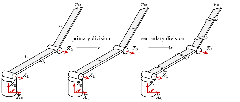
Figure 2: Schematic representation of the setup and of the discretization method.

III-A Modeling

To model the robot, we employ MRFEM [10], which follows a two-step process. First, it divides the flexible links into $n_{\mathrm{seg}}$ segments and lumps their spring and damping properties at one point (primary division). Then, MRFEM isolates so-called rigid finite elements (rfes) between massless passive elastic joints (secondary division), as shown in the Fig. 2. Mechanics textbooks contain ready-to-use formulas for computing inertial properties of the rfes, and spring and damper coefficients for simple geometries. However, for more complex geometries, the use of CAD software becomes necessary.

To derive the equations of motion of a flexible manipulator using the Lagrange method [25, Ch. 7], we denote the vector of joint angles $\bm{q}=[\bm{q}_{\mathrm{a}};\ \bm{q}_{\mathrm{p}}]$, where $\bm{q}_{\mathrm{a}}\in\mathbb{R}^{3}$ represents the active joint angles, and $\bm{q}_{\mathrm{p}}\in\mathbb{R}^{2n_{\mathrm{seg}}}$ represents the passive joint angles. Passive joints are typically implemented as spherical joints to represent compliance in all directions (two bending deformations and a torsional deformation). However, in some cases, such as our setup, compliance predominantly occurs in one direction. In such instances, it is advantageous to simplify the model by only considering flexibility along the most compliant direction. In our setup, we model bending about axes $Z_{1}$ and $Z_{2}$, as shown in Fig. 2. Applying the Lagrange method yields the final expression for the flexible manipulator dynamics discretized using MRFEM

$$\bm{M}(\bm{q})\ddot{\bm{q}}+\bm{C}(\bm{q},\dot{\bm{q}})\dot{\bm{q}}+\bm{K}\bm{q}+\bm{D}\dot{\bm{q}}+\bm{g}(\bm{q})=\bm{B}\bm{\tau},$$ (3)

where $n_{\mathrm{rb}}=1+2(n_{\mathrm{seg}}+1)$; $\bm{M}\in\mathbb{R}^{n_{\mathrm{rb}}\times n_{\mathrm{rb}}}$ is the symmetric inertia matrix; $\bm{K}\in\mathbb{R}^{n_{\mathrm{rb}}\times n_{\mathrm{rb}}}$ and $\bm{D}\in\mathbb{R}^{n_{\mathrm{rb}}\times n_{\mathrm{rb}}}$ are the constant diagonal stiffness and damping matrices, respectively; $\bm{C}\in\mathbb{R}^{n_{\mathrm{rb}}\times n_{\mathrm{rb}}}$ is the matrix of centrifugal and Coriolis forces, $\bm{g}\in\mathbb{R}^{n_{\mathrm{rb}}}$ is the vector of gravitational forces, $\bm{B}\in\mathbb{R}^{n_{\mathrm{rb}}\times 3}$ is the constant control jacobian and $\bm{\tau}\in\mathbb{R}^{3}$ is the torque vector. The model is converted to state-space form by defining $\bm{x}:=\left[\bm{q};\dot{\bm{q}}\right]$ and $\bm{u}:=\bm{\tau}$

$$\dot{\bm{x}} =\bm{f}(\bm{x},\bm{u},n_{\mathrm{seg}})$$ (4)

$$=\left[\dot{\bm{q}};\ \bm{M}(\bm{q})^{-1}\{\bm{B}\bm{\tau}-\bm{C}(\bm{q},\dot{\bm{q}})\dot{\bm{q}}-\bm{K}\bm{q}-\bm{D}\dot{\bm{q}}-\bm{g}(\bm{q})\}\right].$$

The output map of the system is $\bm{y}=[\bm{q}_{\mathrm{a}};\dot{\bm{q}}_{a};\bm{p}_{\mathrm{ee}}]$ where $\bm{p}_{\mathrm{ee}}$ is the EE position.

III-B Simulation and discretization

Roboticists favor MRFEM because existing efficient tools for rigid-body dynamics can be reused: the articulated body algorithm (ABA) for forward dynamics and the recursive Newton-Euler algorithm (RNEA) for the inverse dynamics [26]. In this paper, we use ABA for the forward dynamics and the forward path of the RNEA for the forward kinematics, both generated by Pinocchio [27] as CasADi [28] functions.

As ODE (4) is stiff, commonly used explicit fixed-step integrators in optimal control, e.g. $4$th order Runge-Kutta integrator, quickly diverge. Implicit integrators, although more computationally intensive, offer accurate integration of (4). In this paper, for simulation, we use the backward differentiation formula as implemented in CVODES [29] with specified absolute and relative tolerances. As ground truth dynamics, we consider the model with $n_{\mathrm{seg}}=10$.

III-C Flexible robot environment

Our investigation necessitates an environment for training IL algorithms to approximate $\bm{\pi}_{\mathrm{NMPC}}$. We developed a custom Gym Environment that incorporates the ground truth dynamics of the flexible robot, as specified in the previous subsection. In addition to the robot, this environment features a wall, which serves both to mimic an industrial setting (where constraints like these are commonly encountered) and to represent a safety-critical constraint along with the ground. Both, the wall and the ground constraint form the feasible set $\mathcal{F}(\sigma)$ in the shape of a wedge, i.e., a convex set that results from the intersection of two half spaces. This feasible set can be written as

$$\begin{split}\mathcal{F}(\sigma)=\left\{\bm{p}\in\mathbb{R}^{3}\middle|\begin{array}[]{@{}r@{}}\bm{w}_{\mathrm{wall}}^{\top}(\bm{p}-\bm{b}_{\mathrm{wall}})\geq-\sigma\\ \bm{w}_{\mathrm{ground}}^{\top}(\bm{p}-\bm{b}_{\mathrm{ground}})\geq-\sigma\end{array}\right\},\end{split}$$ (5)

where $\sigma\geq 0$ can be a slack parameter that is used for numerical robustness in optimization algorithms and which is zero in the optimal solution. Hyperplane parameters for the wall are defined by $\bm{w}_{\mathrm{wall}}=[0\ 1\ 0]^{\top}$ and $\bm{b}_{\mathrm{wall}}=[0\ -0.15\ 0.5]^{\top}$ and for the ground by $\bm{w}_{\mathrm{ground}}=[0\ 0\ 1]^{\top}$ and $\bm{b}_{\mathrm{ground}}=[0\ 0\ 0]^{\top}$, respectively.

Given that the value of $n_{\mathrm{seg}}$ may vary between the control model and the simulation model, and considering the presence of simulated measurement noise, we equipped the environment with a state estimator, specifically a discrete-time Extended Kalman Filter (EKF). It infers the states of the control model from the outputs $\bm{y}$ of the simulation model. The EKF leverages the flexible robot model and utilizes automatic differentiation, which is available in CasADi, to linearize the model. In summary, the observation $\bm{o}$ provided by the environment consists of the estimated state $\bm{\hat{x}}$, the current and goal positions of the end-effector $\bm{p}_{\mathrm{ee}}$ and $\bm{p}_{\mathrm{ee,goal}}$, respectively, as well as the hyperplane representation of the wall, denoted by $\bm{w}$ and $\bm{b}$.

IV Implementation

This section details NMPC and safety filter formulations of the proposed framework, and discusses the model discretization sufficient for those components. In addition, the section compares different IL methods for approximating NMPC.

IV-A Expert NMPC

In addition to the generic NMPC of Sec. II-A, we define the controlled output of the robot as algebraic variables $\bm{Z}=\left[\bm{z}_{0},\ldots,\bm{z}_{N}\right]\in\mathbb{R}^{n_{z}\times N}$ which is the Cartesian coordinates of the EE $\bm{z}:=\bm{p}_{\mathrm{ee}}(\bm{x})\in\mathbb{R}^{3}$. The cost function penalizes the deviation from the EE reference $\bm{z}^{\mathrm{ref}}=\bm{p}^{\mathrm{ref}}_{\mathrm{ee}}(\bm{x})$, and as an regularization, also the reference state $\bm{x}^{\mathrm{ref}}$ and reference torque $\bm{u}^{\mathrm{ref}}$ using an $L^{2}$ norm. Given the EE position, the reference states and and controls are approximately computed via the inverse kinematics of a low dimensional approximation of the robot.

To discretize the continuous time system dynamics, a four-stage implicit Runge–Kutta method with a sampling time $\Delta t\ \mathrm{ms}$ was employed, resulting in the equality constraints $\bm{0}=\bm{\Phi}(\bm{x}_{k+1},\bm{x}_{k},\bm{u}_{k})$. Upper $\overline{\bm{u}}$ and lower $\underline{\bm{u}}$ bounds on controls (torques), the upper $\overline{\bm{x}}^{\mathrm{tr}}$ and lower $\underline{\bm{x}}^{\mathrm{tr}}$ bounds on states (joint angles and velocities) were formulated as box constraints. Safety critical bounds were formulated for the EE and elbow positions by $\bm{p}_{\mathrm{ee}}(\bm{x})\in\mathcal{F}(\sigma^{\mathrm{ee}})$ and $\bm{p}_{\mathrm{elb}}(\bm{x})\in\mathcal{F}(\sigma^{\mathrm{elb}})$ (5) using the slack variables $\sigma^{\mathrm{ee}}\in\mathbb{R}$ and $\sigma^{\mathrm{elb}}\in\mathbb{R}$. To avoid constraint violation due to noisy measurements and the model mismatch, we performed a simple heuristic-based constraint tightening via slack variables. In particular, based on the knowledge about the measurement noise, we assumed a safety margin $\bm{\delta}_{x}\in\mathbb{R}^{x}$ for the state constraints $\overline{\bm{x}}=\overline{\bm{x}}^{\mathrm{tr}}-\bm{\delta}_{x}$, $\underline{\bm{x}}=\underline{\bm{x}}^{\mathrm{tr}}+\delta_{x}$, and $\bm{\delta}_{\mathrm{ee}}$ and $\bm{\delta}_{\mathrm{elbow}}$ for the output and elbow constraints, respectively. The tightening of the output and elbow constraints are implemented by setting bounds on the slack variables $\sigma^{\mathrm{ee}}$ and $\sigma^{\mathrm{elbow}}$, respectively.

State and obstacle constraints were formulated using slack variables $\bm{\Sigma}=[\bm{\sigma}_{0},\ldots,\bm{\sigma}_{N}]^{\top}\in\mathbb{R}^{3\times N}$, with $\bm{\sigma}_{k}=[\sigma_{k}^{x}\quad\sigma_{k}^{\mathrm{ee}}\quad\sigma_{k}^{\mathrm{elbow}}]^{\top}\in\mathbb{R}^{3}$, which were penalized in the cost function by $L^{1}$- and squared $L^{2}$-norms (by weights $\bm{s}\in\mathbb{R}^{3}$ and $\bm{S}\in\mathbb{R}^{3\times 3}$, respectively). The matrix $\Delta=[0\ \delta_{\mathrm{ee}}\;\delta_{\mathrm{elbow}}]\otimes\bm{1}_{1\times N}$, which repeats the vector $[0\;\delta_{\mathrm{ee}}\;\delta_{\mathrm{elbow}}]$ for $N$ times, was used to formulate the slack bounds concisely.

Since the optimization problem was formulated for a finite horizon, a simple safe terminal set was used to guarantee recursive feasibility. A safe set of zero angular velocities was chosen and formulated with the matrix $\bm{H}$ that selects the angular velocity states $\dot{\bm{q}}=\bm{H}\bm{x}$ of the state vector $\bm{x}$ and written as $S^{t}=\{\bm{x}\in\mathbb{R}^{n_{x}}|\bm{H}\bm{x}=0\}.$ Notably, the constraints on the positions were already formulated for each stage, thus do not need to be included in the terminal safe set. With the estimated state $\hat{\bm{x}}$, the final nonlinear program reads as [3] X,U,Z,Σ L(X,U,Z,Σ) x_0= ^x,  Σ+Δ≥0,x_N∈S^t 0= F(x_k+1,x_k,u_k), k=0,…,N-1 z_k=[p_ee(x)^⊤,p_elbow(x)^⊤]^⊤, k=0,…,N x -σ_k^x≤x_k ≤¯x +σ_k^x, k=0,…,N u ≤u_k ≤¯u , k=0,…,N-1 p_ee(x)∈F(σ^ee), k=0,…,N p_elbow(x)∈F(σ^elbow), k=0,…,N

where the objective function is

$$L(\bm{X},\bm{U},\bm{Z},\bm{\Sigma})=\sum_{k=0}^{N-1}\left\lVert\bm{x}_{k}-\bm{x}^{\mathrm{ref}}\right\rVert_{\bm{Q}}^{2}+\left\lVert\bm{u}_{k}-\bm{u}^{\mathrm{ref}}\right\rVert_{\bm{R}}^{2}+$$

$$\left\lVert\bm{z}_{k}-\bm{z}^{\mathrm{ref}}\right\rVert_{\bm{P}}^{2}+\left\lVert\bm{\sigma}_{k}\right\rVert_{\bm{S}}^{2}+\left\lVert\bm{\sigma}_{k}\right\rVert_{1,s}+\left\lVert\bm{x}_{N}-\bm{x}^{\mathrm{ref}}_{N}\right\rVert_{\bm{Q}_{N}}^{2}+$$

$$\left\lVert\bm{z}_{N}-\bm{z}^{\mathrm{ref}}\right\rVert_{\bm{P}_{N}}^{2}+\left\lVert\bm{\sigma}_{N}\right\rVert_{\bm{S}}^{2}+\left\lVert\bm{\sigma}_{N}\right\rVert_{1,s},$$ (6)

with $\bm{Q}=\mathrm{diag}(\bm{q})\in\mathbb{R}^{n_{x}\times n_{x}}$, $\bm{R}=\mathrm{diag}(\bm{r})\in\mathbb{R}^{n_{u}\times n_{u}}$ and $\bm{P}=\mathrm{diag}(\bm{p})\in\mathbb{R}^{n_{z}\times n_{z}}$ being stage cost weighting matrices; and $\bm{Q}_{N}\in\mathbb{R}^{n_{x}\times n_{x}}$ and $\bm{P}_{N}\in\mathbb{R}^{n_{z}\times n_{z}}$ being terminal cost weighting matrices. For solving (IV-A), we used the real-time NMPC solver acados [21] with the high performance QP solver HPIPM [30]. The parameters of the NMPC are provided in the projects repository.

To analyze the influence of the model fidelity, i.e., the number of segments, on the controller performance, we compared the NMPC for $n_{\mathrm{seg}}=\{0,1,2,3,5,10\}$. The performance was evaluated by measuring the computation time $t_{\mathrm{MPC}}$, the time $t_{\mathcal{G}_{\epsilon}}$ that NMPC needed to steer the EE into an epsilon ball $\left\lVert\bm{z}(t)-\bm{z}^{\mathrm{ref}}\right\rVert\leq\epsilon$ around the reference position $\bm{z}^{\mathrm{ref}}$ ($\epsilon=10^{-3}$ in our case) and the distance

$$d_{\mathcal{G}_{\epsilon}}=\min_{d}\left\lVert\bm{z}(t)-\bm{z}^{\mathrm{ref}}\right\rVert\leq d\quad\quad\mathrm{s.t.}\;t\geq 3\mathrm{s}.$$ (7)

For $\{0,1\}$ segments, the solver did not converge and for ten segments, the computation time was unacceptably long. As shown in Tab. I, the average mean computation time $\bar{t}_{\mathrm{MPC}}$ and the maximum computation time $t_{\mathrm{MPC}}^{\mathrm{max}}$ increase drastically with the number of segments. However, the performance measured in terms of $t_{\mathcal{G}_{\epsilon}}$ and $d_{\mathcal{G}_{\epsilon}}$ does not significantly improve. Therefore, we selected $n_{\mathrm{seg}}=3$ as a compromise between performance and computation time for for further use with IL algorithms.

$n_{\text{seg}}$	$d_{{\mathcal{G}_{\epsilon}}}/d_{{\mathcal{G}_{\epsilon}}}^{*}$	$t_{{\mathcal{G}_{\epsilon}}}/t_{{\mathcal{G}_{\epsilon}}}^{*}$	$\bar{t}_{\mathrm{MPC}}/\bar{t}_{\mathrm{MPC}}^{*}$	$t_{\mathrm{MPC}}^{\mathrm{max}}/t_{\mathrm{MPC}}^{\mathrm{max},\ *}$
$3$	$1.008$	$0.955$	$1.653$	$1.589$
$5$	$1.026$	$0.974$	$2.95$	$2.940$

TABLE I: Performance comparison of NMPC controllers with different models. Evaluation metrics are measured relative to the NMPC with $n_{\mathrm{seg}}=2$, denoted with superscript ^∗.

IV-B Safety filter

As briefly mentioned in Section II, safety filter can be interpreted as an implicit formulation of the safe set, which is closely related to the formulation of an NMPC. However, since the safety filter is used only for projecting NN control actions into a safe set, the model it uses can be simpler, faster to integrate and the prediction horizon shorter. The proposed safety filter policy ${\bm{\pi}_{\mathrm{SF}}:\mathbb{R}^{n_{u}}\times\mathbb{R}^{n_{x}}\rightarrow\mathbb{R}^{n_{u}}}$ projects the NN output $\bm{u}_{\mathrm{NN}}\in\mathbb{R}^{n_{u}}$ to a safe control $\bm{u}_{\mathrm{SF}}=\bm{\pi}_{\mathrm{SF}}(\bm{x}_{\mathrm{SF}},\bm{u}_{\mathrm{NN}})\in\mathcal{U}_{\mathrm{SF}}\subseteq\mathbb{R}^{n_{u}}$ by using the same formulation as in (IV-A), but with modified cost $L_{\mathrm{SF}}$, a lower fidelity model $\bm{x}_{\mathrm{SF},{i+1}}=\bm{\Phi}_{\mathrm{SF}}(\bm{x}_{\mathrm{SF},{i}},\bm{u}_{\mathrm{SF},{i}})$ with just one segment and a shorter horizon.The safety filter cost function

$$\begin{split}L_{\mathrm{SF}}&(\bm{X}_{\mathrm{SF}},\bm{U}_{\mathrm{SF}},\bm{\Sigma}_{\mathrm{SF}})=\\ &\left\lVert\bm{u}_{0}-\bm{u}_{\mathrm{NN}}\right\rVert_{\bar{\bm{R}}}^{2}+\sum_{k=1}^{N_{\mathrm{SF}}-1}\left\lVert\bm{u}_{k}\right\rVert_{\bm{R}_{\mathrm{SF}}}^{2}+\\ &\sum_{k=0}^{N_{\mathrm{SF}}}\left\lVert\bm{x}_{k}-\bm{x}^{\mathrm{ref}}\right\rVert_{\bm{Q}_{\mathrm{SF}}}^{2}+\left\lVert\bm{\sigma}_{k}\right\rVert_{\bm{S}_{\mathrm{SF}}}^{2}+\left\lVert\bm{\sigma}_{k}\right\rVert_{1,s_{\mathrm{SF}}},\end{split}$$ (8a)

mainly penalizes the deviation from the proposed control $\bm{u}_{\mathrm{NN}}$, besides other terms that are used for regularization and numerical robustness.

IV-C Imitation learning

To approximate NMPC, we compared BC [22], DAgger [23] and three IRL methods: GAIL [31] and AIRL [32], and a two-step IRL method. GAIL and AIRL both employ adversarial approaches to jointly learn the reward function and the policy. The two-step IRL method first learns the reward function using kernel density estimation on the expert demonstrations, similar to the approach in [33], then, uses learned reward function to train a SAC agent agent.

For training, a dataset $\mathcal{D}$ of 100 expert demonstrations were collected using NMPC. All algorithms were trained for 2M steps. DAgger additionally collected 500 more demonstrations during its training phase. Every 5000 gradient step, the algorithms were evaluated using three rollouts in order to save the checkpoint with the highest reward. These checkpoints were then used for final evaluations and experiments that are presented in the Section V. Key hyperparameters employed during training are provided in project repository on GitHub due to space constraints.

For comparing IL algorithms, 100 regulation tasks were randomly generated by randomly sampling initial robot configurations and final end-effector positions in a workspace of the robot. Fig. 4 reveals that DAgger by far outperforms all the other algorithms. Based on these results, in the further experiments we use DAgger for approximating NMPC.

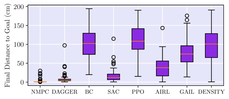
Figure 3: The distribution of the final distance-to-goal of IL and RL algorithms on 100 test tasks.

V SIMULATION EXPERIMENTS

To test the proposed approach, we conducted three different simulation experiments. The first experiment tested the ability of the policies to accomplish the regulation task: reach randomly sampled EE goal position from a randomly sampled initial configuration of the robot. The second experiment tested safety of the policies by randomly sampling the goal position near the obstacle, the wall. The third and final experiment tested the robustness of the policies to the model uncertainty – reduction in the stiffness parameters of the flexible robot by 10%, in particular the $\bm{K}$ matrix in (3). For evaluation, we considered metrics such as the final distance to the goal at the end of each episode/rollout, policy evaluation time (inference time), and the number of constraint violations during an episode.

V-A Reinforcement learning baseline

As a model-free RL baselines, we trained SAC [34] and PPO [35] as strong representatives of offline and online RL algorithms, respectively. Controlling the flexible robot by means of RL is not the main focus of this paper; thus, we did not engineer the reward function $r$. Moreover, reward engineering is difficult in practice and can lead to unintended consequences [36]. Instead, we simply used the Euclidean distance between the robot’s EE and the target EE positions: $r=-\Delta t||\bm{p}_{\mathrm{ee}}-\bm{p}_{\mathrm{ee,goal}}||_{2}$. Both algorithms were trained for 2M gradient steps. When tested on 100 regulation tasks, the SAC considerably outperformed the PPO, as shown in the Fig. 4, therefore, in further experiments only SAC was used.

V-B Results

Closed loop performance:   Fig. 4 reveals that NMPC outperforms all the learning-based algorithms in the output regulation of the flexible robot. Introducing the safety filter significantly decreases the performance of the SAC. One explanation could be the aggressive policy of the SAC, which gets substantially filtered by the more conservative SF to fit within the safe control and state sets. Since DAgger was trained on $\bm{\pi}_{\text{NMPC}}(\bm{\hat{x}})$ demonstrations that fall within the control and state safety sets, its proposed action distribution is similar to that of NMPC. Consequently, the SF modifies the candidate input from DAgger less, resulting in less performance loss compared to SAC.

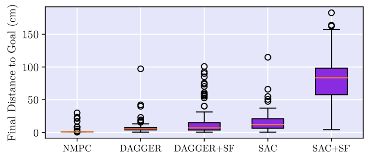
Figure 4: The distribution of final distance-to-goal of IL and RL algorithms on 100 test tasks with and without safety filter

Safety evaluation:   Both the DAgger and SAC algorithms violate critical safety constraints, such as the wall and the ground, as shown in Fig. 5. Importantly, both algorithms operate without explicit awareness of these constraints. RL agents gain knowledge of constraints through a scalar reward function. Since we do not penalize SAC for breaching the constraints, it is more prone to violations. DAgger, on the other hand, implicitly acquires knowledge of constraints from the trajectories of the expert. Through imitation of $\bm{\pi}_{\text{NMPC}}({\bm{\hat{x}}})$, DAgger manages to violate constraints less frequently. The introduction of SF significantly reduces constraint violations, albeit at the cost of decreased performance and increased computation time. SF, however, does not entirely eliminate all constraint violations by SAC, suggesting that when combined with SAC, SF should adopt an even more conservative approach. Regarding computation time, our proposed framework achieves an eightfold reduction in evaluation/computation time compared to NMPC.

Robustness analysis:   Before discussing the results of this experiments, it iss worth pointing out that none of the policies were explicitly trained for robustness. All of them used the nominal model for generating demonstrations $\mathcal{D}$ and for interaction. That said, Fig. 5 shows that changes in stiffness parameters affect both performance and constraint violation frequency. Despite model-plant mismatch, the performance of the expert NMPC remains consistent, but it does violate constraints a few times. Surprisingly, the performance of SAC and SAC combined with SF marginally increases. Similarly, the performance of the proposed framework marginally improves. Constraint violations by DAgger double because the trajectories used for training are not valid on the modified robot.

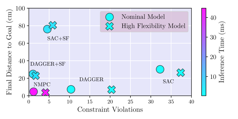
Figure 5: Final distance-to-goal vs constraint violation. Links of the high flexibility model have 10% reduction in their Young’s modulus. The marker colors are defined by the inference time (policy evaluation time).

VI CONCLUSIONS

This work presents a framework for safely approximating NMPC for regulating flexible robots. This framework combines imitation learning, specifically DAgger, which approximates NMPC using a neural network (NN) to significantly reduce the high computation time of NMPC, and a safety filter (SF), formulated as fast and simple NMPC, to ensure obstacle avoidance and constraint satisfaction. We conducted experiments to test the proposed framework using a three degree of freedom flexible manipulator in simulation. Our results demonstrate that DAgger combined with the SF can yield a fast and safe controller. Compared to NMPC, DAgger+SF achieves a remarkable eightfold improvement in computation time. However, this efficiency in policy evaluation comes at a cost in terms of reduced performance. Nonetheless, our framework outperforms conventional reinforcement learning algorithms like SAC, and even SAC combined with SF. When applied to a more flexible robot, DAgger+SF achieves similar performance levels. The proposed approach can be extended to trajectory tracking problems involving flexible robots and control challenges in soft robotics.

References

- [1] W. J. Book, “Recursive lagrangian dynamics of flexible manipulator arms,” The International Journal of Robotics Research, vol. 3, no. 3, pp. 87–101, 1984.
- [2] A. Green and J. Z. Sasiadek, “Dynamics and trajectory tracking control of a two-link robot manipulator,” Journal of Vibration and Control, vol. 10, no. 10, pp. 1415–1440, 2004.
- [3] W. Sunada and S. Dubowsky, “The application of finite element methods to the dynamic analysis of flexible spatial and co-planar linkage systems,” 1981.
- [4] A. A. Shabana, Dynamics of multibody systems. Cambridge university press, 2020.
- [5] T. Yoshikawa and K. Hosoda, “Modeling of flexible manipulators using virtual rigid links passive joints,” International Journal of Robotics Research, vol. 15, no. 3, pp. 290–299, 1996.
- [6] R. Franke, J. Malzahn, T. Nierobisch, F. Hoffmann, and T. Bertram, “Vibration control of a multi-link flexible robot arm with fiber-bragg-grating sensors,” in 2009 IEEE International Conference on Robotics and Automation. IEEE, 2009, pp. 3365–3370.
- [7] P. Staufer and H. Gattringer, “State estimation on flexible robots using accelerometers and angular rate sensors,” Mechatronics, vol. 22, no. 8, pp. 1043–1049, 2012.
- [8] S. Moberg, E. Wernholt, S. Hanssen, and T. Brogårdh, “Modeling and parameter estimation of robot manipulators using extended flexible joint models,” Journal of Dynamic Systems, Measurement, and Control, vol. 136, no. 3, p. 031005, 2014.
- [9] A. Heckmann, “On the choice of boundary conditions for mode shapes in flexible multibody systems,” Multibody System Dynamics, vol. 23, no. 2, pp. 141–163, 2010.
- [10] E. Wittbrodt, I. Adamiec-Wójcik, and S. Wojciech, Dynamics of flexible multibody systems: rigid finite element method. Springer Science & Business Media, 2007.
- [11] B. P. Silva, B. A. Santana, T. L. Santos, and M. A. Martins, “An implementable stabilizing model predictive controller applied to a rotary flexible link: An experimental case study,” Control Engineering Practice, vol. 99, p. 104396, 2020.
- [12] P. Boscariol, A. Gasparetto, and V. Zanotto, “Model predictive control of a flexible links mechanism,” Journal of Intelligent and Robotic Systems, vol. 58, no. 2, pp. 125–147, 2010.
- [13] A. Grancharova and T. Johansen, Explicit Nonlinear Model Predictive Control: Theory and Applications, 03 2012, vol. 429.
- [14] J. Nubert, J. Köhler, V. Berenz, F. Allgöwer, and S. Trimpe, “Safe and Fast Tracking on a Robot Manipulator: Robust MPC and Neural Network Control,” IEEE Robotics and Automation Letters, vol. 5, no. 2, pp. 3050–3057, 2020.
- [15] J. Carius, F. Farshidian, and M. Hutter, “MPC-net: A first principles guided policy search,” IEEE Robotics and Automation Letters, vol. 5, no. 2, pp. 2897–2904, apr 2020.
- [16] L. Brunke, M. Greeff, A. W. Hall, Z. Yuan, S. Zhou, J. Panerati, and A. P. Schoellig, “Safe learning in robotics: From learning-based control to safe reinforcement learning,” Annual Review of Control, Robotics, and Autonomous Systems, vol. 5, no. 1, pp. 411–444, 2022. [Online]. Available: https://doi.org/10.1146/annurev-control-042920-020211
- [17] K. P. Wabersich and M. N. Zeilinger, “A predictive safety filter for learning-based control of constrained nonlinear dynamical systems,” Automatica, vol. 129, no. May, 2021.
- [18] A. P. Vinod, S. Safaoui, A. Chakrabarty, R. Quirynen, N. Yoshikawa, and S. Di Cairano, “Safe multi-agent motion planning via filtered reinforcement learning,” in 2022 International Conference on Robotics and Automation (ICRA), 2022, pp. 7270–7276.
- [19] J. Rawlings, D. Mayne, and M. Diehl, Model Predictive Control: Theory, Computation, and Design, 01 2017.
- [20] H. G. Bock and K.-J. Plitt, “A multiple shooting algorithm for direct solution of optimal control problems,” IFAC Proceedings Volumes, vol. 17, no. 2, pp. 1603–1608, 1984.
- [21] R. Verschueren, G. Frison, D. Kouzoupis, J. Frey, N. van Duijkeren, A. Zanelli, B. Novoselnik, T. Albin, R. Quirynen, and M. Diehl, “acados – a modular open-source framework for fast embedded optimal control,” Mathematical Programming Computation, Oct 2021. [Online]. Available: https://doi.org/10.1007/s12532-021-00208-8
- [22] D. Pomerleau, “Alvinn: An autonomous land vehicle in a neural network,” in Proceedings of (NeurIPS) Neural Information Processing Systems, D. Touretzky, Ed. Morgan Kaufmann, December 1989, pp. 305 – 313.
- [23] S. Ross, G. J. Gordon, and J. A. Bagnell, “A reduction of imitation learning and structured prediction to no-regret online learning,” in AISTATS, 2011.
- [24] J. Malzahn, M. Ruderman, A. Phung, F. Hoffmann, and T. Bertram, “Input shaping and strain gauge feedback vibration control of an elastic robotic arm,” in 2010 Conference on Control and Fault-Tolerant Systems (SysTol). IEEE, 2010, pp. 672–677.
- [25] L. Sciavicco and B. Siciliano, Modelling and control of robot manipulators. Springer Science & Business Media, 2001.
- [26] R. Featherstone, Rigid body dynamics algorithms. Springer, 2014.
- [27] J. Carpentier, G. Saurel, G. Buondonno, J. Mirabel, F. Lamiraux, O. Stasse, and N. Mansard, “The pinocchio c++ library – a fast and flexible implementation of rigid body dynamics algorithms and their analytical derivatives,” in IEEE International Symposium on System Integrations (SII), 2019.
- [28] J. A. E. Andersson, J. Gillis, G. Horn, J. B. Rawlings, and M. Diehl, “CasADi – A software framework for nonlinear optimization and optimal control,” Mathematical Programming Computation, vol. 11, no. 1, pp. 1–36, 2019.
- [29] A. C. Hindmarsh, P. N. Brown, K. E. Grant, S. L. Lee, R. Serban, D. E. Shumaker, and C. S. Woodward, “SUNDIALS: Suite of nonlinear and differential/algebraic equation solvers,” ACM Transactions on Mathematical Software (TOMS), vol. 31, no. 3, pp. 363–396, 2005.
- [30] G. Frison and M. Diehl, “Hpipm: a high-performance quadratic programming framework for model predictive control**this research was supported by the german federal ministry for economic affairs and energy (bmwi) via eco4wind (0324125b) and dyconpv (0324166b), and by dfg via research unit for 2401.” IFAC-PapersOnLine, vol. 53, no. 2, pp. 6563–6569, 2020, 21st IFAC World Congress. [Online]. Available: https://www.sciencedirect.com/science/article/pii/S2405896320303293
- [31] J. Ho and S. Ermon, “Generative adversarial imitation learning,” 2016.
- [32] J. Fu, K. Luo, and S. Levine, “Learning robust rewards with adversarial inverse reinforcement learning,” 2018.
- [33] S. Choi, K. Lee, A. Park, and S. Oh, “Density matching reward learning,” 2016.
- [34] T. Haarnoja, A. Zhou, P. Abbeel, and S. Levine, “Soft actor-critic: Off-policy maximum entropy deep reinforcement learning with a stochastic actor,” 2018.
- [35] J. Schulman, F. Wolski, P. Dhariwal, A. Radford, and O. Klimov, “Proximal policy optimization algorithms,” 2017.
- [36] J. Clark and D. Amodei, “Faulty reward functions in the wild,” 2016. [Online]. Available: https://openai.com/research/faulty-reward-functions