Spontaneous Symmetry Breaking and the Cosmological Constant

Abstract

An approach that allows studying the relationship between the neutralization of the cosmological constant and instantons for cosmology coupled to antisymmetric fields is proposed. Using suitable variables, the Lagrangian leading to the FRW equations can be written analogously to a Ginzburg-Landau theory and we show how spontaneous symmetry breaking appears. The approach leads to three possible solutions, if we denote $\Lambda_{1}$ and $\Lambda_{2}$ as the cosmological constants that come from gravity ($\Lambda_{1}$) and antisymmetric fields ($\Lambda_{2}$), then the solutions, a) $|\Lambda_{2}|>|\Lambda_{1}|$ is consistent with a very small but non-zero $\Lambda_{1}$, b) $|\Lambda_{2}|<|\Lambda_{1}|$, then $\Lambda_{1}$ is observationally ruled out and, c) $|\Lambda_{2}|=|\Lambda_{1}|$ is a solution with finite action and instantons restoring the symmetry $\varphi\to-\varphi$. The third solution is also consistent with neutralization of the cosmological constant in four dimensions.

The problem of the cosmological constant is one of the crucial challenges of modern physics. Its solution, or even a different approach to this problem, can help to understand other cosmological puzzles that until now have not been successfully tackled weinberg ; carroll ; coleman1 . For over forty years, it has been known that the coupling of antisymmetric fields to Einstein’s theory induces an effective cosmological constant nicolai ; duff ; freund which might even be neutralized due to the presence of such fields.

The effective cosmological constant, $\Lambda_{eff}$, must be positive for the universe to accelerate (for a review, see abdalla ). It is composed of different contributions due to the presence of the antisymmetric fields, and such components have opposite signs to make the neutralization occurs. In four dimensions, there are no global obstructions nicolai ; duff ; freund , and the kinetic term of these fields behaves as $\sqrt{g}\,F_{\mu\nu\lambda\rho}F^{\mu\nu\lambda\rho}\sim\Lambda_{2}\,\sqrt{g}$, i.e., producing the effective cosmological constant $\Lambda_{\text{e}ff}=\Lambda_{1}+\Lambda_{2}$.

In higher dimensions the problem is more subtle because the $4$-form $F$ satisfies a generalized Dirac quantization condition Teitelboim ; Bousso and the cosmological constant neutralization problem requires a discrete parameter space.

A first mechanism implementing such ideas has been discussed in nicolai ; duff ; freund for a four-dimensional spacetime. In contrast, a second one, analyzed in ct1 , is defined in higher dimensions containing some of the essential ingredients introduced in Bousso . For other approaches, see for example kaloper0 ; kaloper00 ; kaloper ; otros and references therein.

In this paper, we want to examine the problem of neutralizing the cosmological constant using conventional physics. What does conventional physics mean? It means, surprisingly, that by writing suitably $-\Lambda_{2}\sqrt{-g}$ (the cosmological term coming from $F_{\mu\nu\rho\lambda}F^{\mu\nu\rho\lambda}$ in four dimensions) the cosmological model fits precisely with a Ginzburg-Landau theory, the most prominent description of an effective classical field theory.

In order to explain our results, we begin by considering the Euclidean action of Einstein’s theory

$$S=\int d^{D}x\,\sqrt{-g}\left(R-2\Lambda_{eff}\right)+\cdots.$$ (1)

where $\Lambda_{eff}=\Lambda_{1}+\Lambda_{2}$ and $8\pi G=1$. In the previous expression, the term “$\cdots$ ”  denotes other possible couplings.

Under these conditions, we will show that the cosmological constant can be dynamically adjusted and eventually neutralized.

Let us consider the FRW universe with zero spatial curvature

$$ds^{2}=-N^{2}(t)dt^{2}+a^{2}(t)\left(dx^{2}+dy^{2}+dz^{2}\right),$$ (2)

with $a(t)$ the scale factor and $N(t)$, an auxiliary field that guarantees the invariance of the action under time reparametrization.

The Lagrangian leading to the FRW equations gondolo

$$2\frac{\ddot{a}}{a}+\left(\frac{{\dot{a}}}{a}\right)^{2}+\Lambda_{eff}=0,$$ (3)

$$\left(\frac{\dot{a}}{a}\right)^{2}=\frac{\Lambda_{eff}}{3},$$ (4)

is

$$L=\frac{a{\dot{a}}^{2}}{2N}+\frac{1}{6}\Lambda_{eff}Na^{3}.$$ (5)

It is worth noting that the $\Lambda_{2}$ part contained in $\Lambda_{eff}$ can be obtained from a sort of relativistic membrane, with $\Lambda_{2}$ playing the role of the tension. Indeed, consider the Lagrangian $L_{\Lambda_{2}}=\Lambda_{2}\sqrt{-g}$, which can also be obtained from

$$\tilde{L}_{\Lambda_{2}}=\frac{1}{2\lambda}g+\frac{1}{2}\Lambda^{2}_{2}\lambda,$$ (6)

with $\lambda(t)$ an auxiliary field. The Lagrangian (6) has the advantage of having a smooth $\Lambda_{2}\to 0$ limit and is analogous to the one of the massive relativistic particles in the einbein formulation. Namely $\tilde{L}_{\lambda}=\frac{1}{2\lambda}{\dot{x}}^{2}+\frac{1}{2}m^{2}\lambda$, instead of $L_{\lambda}=-m\sqrt{{-\dot{x}}^{2}}$. Here, $\tilde{L}_{\lambda}$ has the advantage of having a smooth massless limit.

The contribution (6) in the FRW geometry, gives rise to the full Lagrangian

$$L=\frac{a{\dot{a}}^{2}}{2N}+\frac{1}{6}\Lambda_{1}Na^{3}+\frac{1}{12\lambda}a^{6}N+\frac{\Lambda^{2}_{2}}{12}\lambda N,$$ (7)

which, with the change of variables

$$\varphi=\frac{2}{3}a^{\frac{3}{2}},$$ (8)

turns out to be

$$L=\frac{1}{2N}{\dot{\varphi}}^{2}+\frac{3}{8}\Lambda_{1}N\varphi^{2}+\frac{27}{64\lambda}N\varphi^{4}+\frac{1}{12}\Lambda_{2}^{2}\lambda N.$$ (9)

The potential has two minima,

$$\varphi_{0}=\pm\frac{2}{3}\sqrt{-{{\lambda}}\,\Lambda_{1}},$$ (10)

such that perturbations around these minima break the symmetry $\varphi\to-\varphi$.

It is convenient to define $-\mu^{2}=\frac{3}{4}\Lambda_{1}$, and $\frac{\kappa}{4}=\frac{27}{{64}}$. Then eq. 9 becomes

$$L = =\frac{1}{2N}{\dot{\varphi}}^{2}-\frac{\mu^{2}}{2}N\,\varphi^{2}+\frac{\kappa}{4}\,\frac{N}{\lambda}\varphi^{4}+\frac{1}{12}\,N\,\lambda\,\Lambda_{2}^{2},$$ (11)

$$= L_{0}+\frac{1}{12}N\,\Lambda_{2}^{2},$$ (12)

leading to the field equation

$$\frac{d}{dt}\left(\frac{\dot{\varphi}}{N}\right)+\mu^{2}N\,\varphi-\frac{\kappa N}{\lambda}\varphi^{3}=0,$$ (13)

and the reparametrization constraint

$$\frac{{\dot{\varphi}}^{2}}{{{2}}N^{2}}+\frac{\mu^{2}}{2}\varphi^{2}-\frac{\kappa}{4}\varphi^{4}-\frac{\lambda}{12}\Lambda_{2}^{2}=0.$$ (14)

These equations are simplified by choosing the ‘proper-time’ gauge $N=1$, and $\lambda=1$ marti1 to obtain

$${\ddot{\varphi}}+\mu^{2}\,\varphi-\kappa\varphi^{3} = 0,$$ (15)

$$\frac{1}{2}{\dot{\varphi}}^{2}+\frac{\mu^{2}}{2}\varphi^{2}-\frac{\kappa}{4}\varphi^{4}-\frac{1}{12}\Lambda_{2}^{2} = 0.$$ (16)

The first equation has the solution

$$\varphi=\frac{\mu}{\sqrt{\kappa}}\tanh\left[\frac{\mu}{\sqrt{2}}(t-t_{0})\right].$$ (17)

The solutions of the constraint (16), on the other hand, are solutions of (15). Indeed, multiplying this equation by $\dot{\varphi}$, gives rise to

$$\frac{d}{dt}\left[\frac{1}{2}{\dot{\varphi}}^{2}+\frac{\mu^{2}}{2}\varphi^{2}-\frac{\kappa}{4}\varphi^{4}\right]=0,$$

and therefore, $\frac{1}{2}{\dot{\varphi}}^{2}+\frac{\mu^{2}}{2}\varphi^{2}-\frac{\kappa}{4}\varphi^{4}$ is a constant which turns out to be $\mu^{4}/4\kappa$, and must be equal to $\frac{1}{12}\Lambda_{2}^{2}$, imposing the condition $|\Lambda_{1}|=|\Lambda_{2}|$, namely the neutralization of the effective cosmological constant, as we will discuss in what follows.

In Euclidean space, the Lagrangian is the Gibbs free energy (density) and (12) can be viewed in the proper-time gauge as a Ginzburg-Landau theory with the parameters $\mu^{2}$ and $\kappa$ formally as functions of $T$.

Global stability demands that $\kappa>0$ while $\mu^{2}$, according the Ginzburg-Landau theory, becomes $\mu^{2}\to\mu^{2}(T)=\mu^{2}_{0}\left(1-\frac{T}{T_{c}}\right)$, where $\mu_{0}^{2}$ is some function of $T$ although its sign is fixed by the cosmological constant .

In (12), $L_{0}$ is conventional Gibbs free energy while $\frac{1}{12}\Lambda_{2}^{2}$ is analogous to an external field and it does not play any role for the phase transition.

If we take this fact into account, we can choose the combination of parameters $\{\mu^{2},\Lambda_{2}\}$ such that

$$L=\frac{1}{2}{\dot{\varphi}}^{2}+\frac{\kappa}{4}\left(\varphi^{2}-\frac{\mu^{2}}{{{\kappa}}}\right)^{2}+\Delta L[\mu,\Lambda_{2},T],$$ (18)

where

$$\Delta L = -\frac{\mu^{4}}{4\kappa}+\frac{1}{12}\Lambda_{2}^{2}$$ (19)

$$= \frac{1}{12}(\Lambda_{2}^{2}-\Lambda_{1}^{2}).$$

giving rise to the following possibilities

• $\Delta L\geq 0$ implies $|\Lambda_{2}|\geq|\Lambda_{1}|$, therefore, if the cosmological constant $\Lambda_{2}$ is very small, then $\Lambda_{1}$ that comes from the gravity sector should be even smaller (although not zero).

• If $\Delta L\leq 0$ then $|\Lambda_{2}|\leq|\Lambda_{1}|$. This possibility however produces a very large cosmological constant ($\Lambda_{1}$) and is ruled out observationally.

• Finally, $\Delta L=0$ results

  $$\Lambda_{1}=\Lambda_{2}.$$ (20)

  This equation has the consequence that the action $\int_{-\infty}^{\infty}dtL$ is finite and therefore implies the existence of instantons Polyakov ; Coleman . It is the instantons that restore this symmetry breaking $\varphi\to-\varphi$.

In terms of $\Lambda_{2}$ the effective cosmological constant has the following solution

$$-2|\Lambda_{2}|\leq\Lambda_{\text{eff}}\leq 2|\Lambda_{2}|.$$ (21)

which shows that there are regions between $-2|\Lambda_{2}|$ and $2|\Lambda_{2}|$ where $\Lambda_{\text{e}ff}$ is neutralized (see Figure 1).

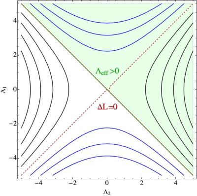
Figure 1: The figure shows a possible qualitative plot of the effective cosmological constant for the three scenarios given by (19). The possibilities show some values of the effective cosmological constant. The green region shows the physical condition $\Lambda_{eff}=\Lambda_{1}+\Lambda_{2}>0$. Black, blue and red show conditions for $\Delta L$. Black lines correspond to $\Delta L>0$, blue shows $\Delta L<0$ and red shows $\Delta L=0$, in the neutralization scenario.

Summarizing, we highlight that if (20) holds, the instantons do the dirty work of restoring the symmetry breaking and provide a novel approach to the question of the neutralization of the cosmological constant.

References

- (1) S. Weinberg, Rev. Mod. Phys. 61 (1989), 1-23.
- (2) S. M. Carroll, Living Rev. Rel. 4 (2001), 1.
- (3) S. R. Coleman, Nucl. Phys. B 310 (1988), 643-668.
- (4) A. Aurilia, H. Nicolai and P. K. Townsend, Nucl. Phys. B 176 (1980), 509-522.
- (5) M. J. Duff and P. van Nieuwenhuizen, Phys. Lett. B 94 (1980), 179-182.
- (6) P. G. O. Freund and M. A. Rubin, Phys. Lett. B 97 (1980), 233-235.
- (7) E. Abdalla, G. Franco Abellán, A. Aboubrahim, A. Agnello, O. Akarsu, Y. Akrami, G. Alestas, D. Aloni, L. Amendola and L. A. Anchordoqui, et al. JHEAp 34 (2022), 49-211.
- (8) C. Teitelboim, Phys. Lett. B 167 (1986), 69-72.
- (9) R. Bousso and J. Polchinski, JHEP 06 (2000), 006.
- (10) J. D. Brown and C. Teitelboim, Phys. Lett. B 195 (1987), 177-182; ibid, Nucl. Phys. B 297 (1988), 787-836.
- (11) N. Kaloper, Phys. Rev. D 106, no.6, 6 (2022).
- (12) N. Kaloper, Phys. Rev. D 106, 4 (2022).
- (13) N. Kaloper and A. Westphal, [arXiv:2204.13124 [hep-th]];
- (14) J. L. Lehners, R. Leung and K. S. Stelle, [arXiv:2209.08960 [hep-th]]; M. Arcos, W. Fischler, J. F. Pedraza and A. Svesko, [arXiv:2207.06447 [hep-th]]; U. Danielsson, D. Panizo and R. Tielemans, Phys. Rev. D 106 (2022) no.2, 024002.
- (15) H. Falomir, J. Gamboa, F. Méndez and P. Gondolo, Phys. Rev. D 96 (2017) no.8, 083534 and ibid, Phys. Lett. B 785 (2018), 399-402.
- (16) T. Eguchi, Phys. Rev. Lett. 44 (1980), 126.
- (17) J. Gamboa and M. Ruiz-Altaba, Phys. Lett. B 205 (1988), 245-249.
- (18) A. Karlhede and U. Lindström, Class. Quant. Grav. 3 (1986), L73-L75.
- (19) F. Lizzi, B. Rai, G. Sparano and A. Srivastava, Phys. Lett. B 182 (1986), 326-330.
- (20) A. M. Polyakov, Nucl. Phys. B 120 (1977), 429-458.
- (21) S. R. Coleman, “The Uses of Instantons”, Subnucl. Ser. 15 (1979), 805 HUTP-78-A004.