amssymb

Response to Comment arXiv:2210.10539v2

In recent work Horváth and Markobs (2022a), we calculated the infrared (IR) effective counting dimension $d_{\scriptscriptstyle{\text{\rm IR}}}$ Horváth and Mendris (2020); Alexandru and Horváth (2021); Horváth et al. (2022) for critical states of $3D$ Anderson models in universality classes O, U, S and AIII. The results entailed two new messages. (m1) Space effectively occupied by critical electron is of dimension $d_{\scriptscriptstyle{\text{\rm IR}}}\!\approx\!8/3$. Demonstrated properties of effective counting imply that the meaning and relevance of this is fully analogous to e.g. Minkowski dimension of ternary Cantor set being $d_{\scriptscriptstyle{\text{\rm UV}}}\!=\!\log_{3}(2)$. Indeed, both statements express the scaling of properly defined physical volume; both dimensions are measure-based. (m2) The values of $d_{\scriptscriptstyle{\text{\rm IR}}}$ in studied classes coincide to better than two parts per mill with comparable errors. We dubbed this finding superuniversality of $d_{\scriptscriptstyle{\text{\rm IR}}}$ since other critical indices tend to differ to a notably larger degree. Exact superuniversality offers itself as a possibility, but obviously cannot be demonstrated in a finite numerical computation, only ascertained with better bounds or disproved.

In Ref. Burmistrov (2022) Burmistrov claims that he “proved” inexact nature of (m2) by invoking the multifractal (MF) formalism. He derived MF representation for average effective count $\langle\mathscr{N}_{\star}\rangle$, involving $f(3)$ and $\alpha_{0}$ ($f(\alpha_{0})\!=\!3$), namely

$$\langle\mathscr{N}_{\star}\rangle\simeq 4c_{0}\frac{L^{f(3)}}{\sqrt{\ln(L)}}\quad,\quad c_{0}=\sqrt{|f^{\prime\prime}(\alpha_{0})|/(2\pi)}$$ (1)

The asymptotically equal sign ($\,\simeq\,$) suggests that (1) conveys an exact $L\!\to\!\infty$ leading term of $\langle\mathscr{N}_{\star}\rangle$. However, in the ensuing discussion, $4c_{0}$ appears to be treated as approximation to proportionality constant, which is what we will assume. Burmistrov then concludes that (1) “proves the absence of “superuniversality” of $\langle\mathscr{N}_{\star}\rangle$” due to numerically known class-dependent values of $f(3)$ and $c_{0}$. We note in passing that superuniversality of $\langle\mathscr{N}_{\star}\rangle$, exact or not, was in fact not claimed or invoked in Horváth and Markobs (2022a).

To put formula (1) in context, recall that MF formalism was created to describe UV measure singularities arising e.g. in strange attractors Falconer (2014); Halsey et al. (1986). The method identifies sets $A_{\alpha}$ of local singularities with Hölder strength $\alpha\!>\!0$, treating their Hausdorff dimensions $f_{H}(\alpha)\!=\!\text{dim}_{H}(A_{\alpha})$ as characteristics of interest. Note that $f_{H}(\alpha)$ is a proper measure-based dimension of spatial set $A_{\alpha}$.

Common variation is the moment method which avoids computing $\alpha(x)$ at each point for the price of coarsening the singularity information. Evaluation of the associated $f_{m}(\alpha)$ proceeds by computing continuum of generalized dimensions which are not measure-based and do not represent dimensions of space in themselves. Nevertheless, $f_{H}(\alpha)$ and $f_{m}(\alpha)$ coincide under certain analytic assumptions by virtue of associated transformations. However, the moment method does not identify the singularity set $A_{\alpha}$. What it does provide is a trick to evaluate $f_{H}(\alpha)$ valid in certain circumstances. Without explicit check that $f_{H}(\alpha)\!=\!f_{m}(\alpha)$ or explicit verification that needed analytic properties are met, one has no choice but to treat $f_{m}(\alpha)$ as approximation to $f_{H}(\alpha)$.

In Anderson criticality, the situation is somewhat different. This is an IR problem which means that the notion of local singularity is absent and the very concept of $A_{\alpha}$ becomes fuzzy. The moment method is then normally taken to define MF spectrum $f(\alpha)\!\equiv\!f_{m}(\alpha)$ upon formally replacing the UV cutoff $a$ with $1/L$. However, one is left with little regarding the information on populations (subsets of space) whose dimensions is $f_{m}(\alpha)$ meant to represent. Unlike in UV problem of a strange attractor, there is no readily available analogue of $A_{\alpha}$ and $f_{H}(\alpha)$ to independently check upon.

Formula (1) may prove valuable in this regard since it represents MF prediction ($f\!\equiv\!f_{m}$) for $\langle\mathscr{N}_{\star}\rangle$ which has independent definition and well-defined spatial meaning. Degree of consistency between true $\langle\mathscr{N}_{\star}\rangle$ and (1) can thus test assumptions associated with the MF approach. We perform such comparison to $\langle\mathscr{N}_{\star}\rangle$ data of Ref. Horváth and Markobs (2022a). To minimize finite-$L$ systematics, only the upper segment of all data ($64\leq L\leq 128$) is used to fit for $c_{0}$ and $f(3)$. We find that instead of improving, fit form (1) worsens $\chi^{2}$/dof relative to pure power ($1.5\rightarrow 2.9$). More importantly, resulting $f(3)$ is sharply inconsistent with the MF-computed value $f(3)\!=\!2.733(3)$ Ujfalusi and Varga (2015), used in Burmistrov argument. Described results refer to O class but situation in other classes is the same.

The above is conveyed by Fig. 1(a) where $1/L$ behavior of $f(3)$, expressed from Eq. (1), is shown together with fitted $1/L\!=\!0$ value (with error) and the associated MF prediction. Analogous plot for pure power is also shown (full circles). Fitted $d_{\scriptscriptstyle{\text{\rm IR}}}$ here is consistent with one obtained from the extrapolated pair method Horváth and Markobs (2022a). Approach of data to fitted values in both cases is of course by design, similarly to plots in Fig. 1 of Ref. Burmistrov (2022). Note also that the obtained $c_{0}$ differs roughly by factor of two from its approximate MF prediction as shown in Fig. 1(b).

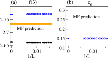
Figure 1: MF-computed indices $f(3)$ Ujfalusi and Varga (2015) and $c_{0}$ compared to those obtained from Eq. (1) and $\langle\mathscr{N}_{\star}\rangle$ data of Ref. Horváth and Markobs (2022a).

The above discussion warrants the following points.

(i) Given the scale of inconsistencies found in the MF prediction (1), we conclude that arguments of Ref. Burmistrov (2022) do not have tangible bearing on our (m1) and (m2), including the possibility of exact superuniversality in $d_{\scriptscriptstyle{\text{\rm IR}}}$. One should also keep in mind that superuniversality and $d_{\scriptscriptstyle{\text{\rm IR}}}\!\approx\!8/3$ are two distinct conclusions.

(ii) Our findings suggest that derivation of (1) may involve assumptions on $\alpha$-populations that are not justified. For example, setting $p(x)\!\equiv\!L^{-\alpha(x)}$ ($p(x)=\,$probability at $x$), which forces certain structure on $\alpha$-populations without knowing what they actually are, may be too cavalier. Showing that this is harmless in $L\!\to\!\infty$ limit is non-trivial even for moderately complex populations. Similar goes for setting ${\cal P}(\alpha)\!\equiv\!{\cal C}L^{f(\alpha)}$ where ${\cal P}(\alpha)$ is the $\alpha$-population count. Assumptions on analyticity of $f(\alpha)$, $f_{m}(\alpha)$ and quadratic local nature of maximum at $\alpha_{0}$ are also present. Characterizations such as “exact” and “proof” in this context are perhaps too strong and premature.

(iii) Arguments of Burmistrov (2022), leading to claim of systematic effect in the analysis of Horváth and Markobs (2022a), use numerical results of Ujfalusi and Varga (2015). But systematics involved in the latter work is not discussed although smaller systems and smaller statistics were used. (Systematics in Horváth and Markobs (2022a) was also studied in Ref. Horváth et al. (2022) albeit from a different angle.) Are there logs affecting standard MF analyses, appearing e.g. via arbitrary replacement $p\!\equiv\!L^{-\alpha}\rightarrow p\!\equiv\!\text{const}\,L^{-\alpha}$. Are they accounted for?

(iv) The presence of $\log(L)$ powers in dimension estimates is always possible since they leave it intact. MF arguments are not necessary to invoke the possibility. But in the absence of a firm prediction, establishing their presence is a delicate numerical issue. Indeed, it is difficult to show that the influence of an unknown $\log$ is larger than that of subleading powers. Statistical strength of available data is frequently not sufficient to do that. Occam’s razor approach is then an accepted resolution.

(v) We strongly disagree with the comment “$d_{\scriptscriptstyle{\text{\rm IR}}}$ is nothing but f(d)”. There was also a calculus student who once declared “$\pi$ is nothing but $\,22/7\!-\!\int_{0}^{1}dx\,x^{4}(1-x)^{4}/(1+x^{2})$”. Perhaps there is a bit more to $d_{\scriptscriptstyle{\text{\rm IR}}}$ than the currently hypothetical $d_{\scriptscriptstyle{\text{\rm IR}}}\!=\!f_{m}(3)$. Its meaning is expressed in (m1), being worked out in requisite detail by Refs. Horváth and Mendris (2020); Alexandru and Horváth (2021); Horváth et al. (2022).

(vi) Regarding comments on prospects for superuniversality in various dimensions, we repeat that our claim is only for $d_{\scriptscriptstyle{\text{\rm IR}}}$ at level better than two parts per mill in $D\!=\!3$. The gist of our message is that properties of space in Anderson transitions may be special relative to other characteristics. Scenario where superuniversality in $d_{\scriptscriptstyle{\text{\rm IR}}}$ is violated in $D\!=\!2+\epsilon$ but very accurate or exact in $D\!=\!3$ and higher dimensions is not contradictory in our opinion.

RESPONSE TO ADDENDUM

New material was added to Ref. Burmistrov (2022) in version 2. Its focus is to suggest that inconsistencies found in originally proposed approximation (1) of $\langle\mathscr{N}_{\star}\rangle_{L}$ are rectified by the use of full integral formula Burmistrov (2022) ($f_{m}$ from moment method)

$$\langle\mathscr{N}_{\star}\rangle_{L}^{m}\equiv\sqrt{2\ln(L)|f^{\prime\prime}_{m}(\alpha_{0})|/\pi}\,\int_{-\infty}^{D}d\alpha\,L^{f_{m}(\alpha)}$$ (2)

More precisely, although it is admitted that $\langle\mathscr{N}_{\star}\rangle_{L}^{m}$ is not a good theory of $\langle\mathscr{N}_{\star}\rangle_{L}$, even in its full form (2), it is claimed to provide an accurate theory of $d_{\scriptscriptstyle{\text{\rm IR}}}(L,2)$ Horváth and Markobs (2022a) (see (3) below). We will show that this is not the case when associating $d_{\scriptscriptstyle{\text{\rm IR}}}$ with $f_{m}(3)\!=\!2.733(3)$ as hypothesized in Burmistrov (2022). In the second part we give further support to conclusions of Ref. Horváth and Markobs (2022a) and propose the resolution of inconsistencies between $d_{\scriptscriptstyle{\text{\rm IR}}}$ and its representation via $f_{m}$, revealed by our analysis.

Discussion in ADDENDUM avoids elaborating on ramifications of standard MF variable choice $p(x)\equiv L^{-\alpha(x)}$, raised by our point (ii). To be able to discuss related issues further, we thus adopt it as a defining attribute of MF approach in what follows. The framework then seeks to determine the dimension function $f(\alpha)$ associated with $\alpha$-based partition of (lattice) space $\Omega(L)$. More precisely, let $A(\alpha,L,\psi)$ be the subset of points $x$ for which $\psi^{+}\psi(x)\!=\!L^{-\alpha}$ so that $\Omega(L)=\cup_{\alpha}A(\alpha,L,\psi)$, and ${\cal P}(\alpha,L,\psi)$ the count of these points Burmistrov (2022). Here $\psi$ is a critical Anderson state. Like in the UV case of fixed sets, $f(\alpha)$ aims to represent the dimension of set $A(\alpha)$. The stochastic nature of $A(\alpha,L,\psi)$ then forces the definition be based on IR scaling of average counts ${\cal P}(\alpha,L)\equiv\langle{\cal P}(\alpha,L,\psi)\rangle$. We emphasize that we now strictly distinguish $f(\alpha)$, constructed as above, from $f_{m}(\alpha)$ of the moment method which is its (sometimes exact) approximation.

Given this setup, $\langle\mathscr{N}_{\star}\rangle_{L}\!=\!\int d\alpha\,{\cal P}(\alpha,L)\min\{1,L^{D-\alpha}\}$ of Ref. Burmistrov (2022) holds, and $\langle\mathscr{N}_{\star}\rangle_{L}$ is encoded in ${\cal P}(\alpha,L)$. However, it is not fully encoded in $f(\alpha)$. Similarly, the finite-$L$ IR dimension $d_{\scriptscriptstyle{\text{\rm IR}}}(L)\!\equiv\!d_{\scriptscriptstyle{\text{\rm IR}}}(L,s\!=\!2)$, namely Horváth and Markobs (2022a)

$$d_{\scriptscriptstyle{\text{\rm IR}}}(L)\!=\!\frac{1}{\ln(2)}\ln\frac{\langle\mathscr{N}_{\star}\rangle_{L}}{\langle\mathscr{N}_{\star}\rangle_{L/2}}\quad,\quad d_{\scriptscriptstyle{\text{\rm IR}}}\!=\!\lim_{L\to\infty}d_{\scriptscriptstyle{\text{\rm IR}}}(L)$$ (3)

is encoded in ${\cal P}(\alpha,L)$ but not in $f(\alpha)$ alone. Before expressing the relationship of $f(\alpha)$ and $d_{\scriptscriptstyle{\text{\rm IR}}}$, we first emphasize that the definition of $d_{\scriptscriptstyle{\text{\rm IR}}}$ indicated in (3) does not only apply to pure powers as claimed in Burmistrov (2022), but generally. Indeed, it returns $d_{\scriptscriptstyle{\text{\rm IR}}}$ for all $\langle\mathscr{N}_{\star}\rangle_{L}\!=\!L^{d_{\scriptscriptstyle{\text{\rm IR}}}}h(L)$ where $h(L)$ varies slower than any non-zero power near $L\!=\!\infty$, which is the usual meaning of Minkowski-like dimension. For example, linearly extrapolated $d_{\scriptscriptstyle{\text{\rm IR}}}(L)$ of Horváth and Markobs (2022a) corresponds to asymptotic behavior $L^{d_{\scriptscriptstyle{\text{\rm IR}}}}\exp(c/L)$.

Applying now the same rational to $f(\alpha)$ and its associated $f(\alpha,L)\equiv f(\alpha,L,s\!=\!2)$ results in

$$\langle\mathscr{N}_{\star}\rangle_{L}\!=\!\int_{-\infty}^{\infty}d\alpha\,v(\alpha,L)\,L^{f(\alpha,L)}\,\min\{1,L^{D-\alpha}\}$$ (4)

Here functions $v(\alpha,L)$, $f(\alpha,L)$ are constructed from

$$f(\alpha,L,\epsilon)=\frac{1}{\ln(2)}\,\ln\frac{{\cal P}(\alpha,L,\epsilon)}{{\cal P}(\alpha,L/2,\epsilon)}$$ (5)

where ${\cal P}(\alpha,L,\epsilon)$ is the count in interval $(\alpha-\epsilon,\alpha]$, via

$$f(\alpha,L)\!=\!\lim_{\epsilon\to 0}f(\alpha,L,\epsilon)\;\;,\;\;v(\alpha,L)\!=\!\lim_{\epsilon\to 0}\frac{{\cal P}(\alpha,L,\epsilon)}{\epsilon\,L^{f(\alpha,L,\epsilon)}}\;$$ (6)

The rewrite (4) of $\langle\mathscr{N}_{\star}\rangle_{L}$ caters to MF variable $\alpha$ and is exact if limits in (6) exist. In general, there may be non-analyticities already at finite $L$. The multifractal singularity spectrum is defined by $f(\alpha)=\lim_{L\to\infty}f(\alpha,L)$. We emphasize again that $v(\alpha,L)$ that is finite and nonzero for all sufficiently large $L$ may still tend to $0$ or $\infty$ for $L\to\infty$, albeit slower than any non-zero power of $L$.

Formula (4) connects $d_{\scriptscriptstyle{\text{\rm IR}}}$ and $f(\alpha)$ most generally. Under rather mild conditions on uniform convergence of $f(\alpha,L)$ it translates into

$$d_{\scriptscriptstyle{\text{\rm IR}}}\!=\sup\{\,\{f(\alpha)\!\mid\!\alpha\leq D\}\,\cup\,\{f(\alpha)\!+\!D\!-\!\alpha\!\mid\!\alpha>D\}\,\}\;$$ (7)

This representation applies in any context with well-defined $f(\alpha)$ and it is a nice contribution of Ref. Burmistrov (2022) to spark this connection. However, using it in practice amounts to “putting the cart before the horse” unless a precise $f(\alpha)$ is available, which is very rare.

For 3D Anderson criticality problem, it is reasonable to expect that (7) will eventually yield $d_{\scriptscriptstyle{\text{\rm IR}}}=f(3)$, but $f(\alpha)$ has not been computed yet. Rather, the MF framework is replaced by an approximation afforded by the moment method. Such mMF formalism substitutes $f(\alpha)$ with $f_{m}(\alpha)$ defined by generalized dimensions via Legendre transform, and assigns identical weight to distinct $\alpha$-populations, namely

$$v(\alpha,L)\,L^{f(\alpha,L)}\quad\longrightarrow\quad{\cal C}(L)\,L^{f_{m}(\alpha)}$$ (8)

in all expressions, including Eq. (4). For this to be consistent, some features that are automatic in MF have to be explicitly imposed in mMF, in particular the normalization of counts and the wave function

$$\frac{1}{{\cal C}(L)}=\int_{-\infty}^{\infty}d\alpha\,L^{f_{m}(\alpha)-D}=\int_{-\infty}^{\infty}d\alpha\,L^{f_{m}(\alpha)-\alpha}$$ (9)

Arguments in Burmistrov (2022) leading to $d_{\scriptscriptstyle{\text{\rm IR}}}\!=\!f_{m}(D)$ also rely on Mirlin et al. (2006)

$$f_{m}(2D-\alpha)=f_{m}(\alpha)+D-\alpha$$ (10)

which thus has to be imposed in this particular analysis as well. We can now discuss the merits of mMF approximations to $d_{\scriptscriptstyle{\text{\rm IR}}}(L)$.

Parabolic mMF. It is easy to check that, given $\alpha_{0}$, the only parabolic $f_{m}(\alpha)$ satisfying (10) is

$$f_{m}^{p}(\alpha)=D-\frac{1}{4}\frac{(\alpha-\alpha_{0})^{2}}{\alpha_{0}-D}\quad,\quad\alpha_{0}>D$$ (11)

which also satisfies conditions (9) at each $L$. Therefore

$$f_{m}^{p}(D)=D-\frac{\alpha_{0}-D}{4}\;\longrightarrow\;f_{m}^{p}(3)=2.739$$ (12)

for $D\!=\!3$ and $\alpha_{0}\!=\!4.043$. This is thus the prediction for $d_{\scriptscriptstyle{\text{\rm IR}}}$ by mMF in parabolic approximation. Note that $\alpha_{0}$ is quoted in Burmistrov (2022) without error. The associated $d_{\scriptscriptstyle{\text{\rm IR}}}(L)$ given by master mMF formula (2) is shown in Fig.2 together with numerical data. We have extended the range of studied lattices and their statistics for this purpose. The obvious disagreement of the theory with the data makes the parabolic mMF prediction $d_{\scriptscriptstyle{\text{\rm IR}}}\!=\!2.739$ unreliable.

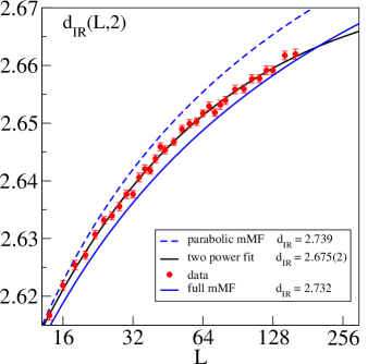
Figure 2: Parabolic (dashed blue) and full (blue) mMF predictions for $d_{\scriptscriptstyle{\text{\rm IR}}}(L)$ vs true values (data). Dependence from 2-power fits of $\langle\mathscr{N}_{\star}\rangle_{L}$ in corresponding range of $L$ is also shown.

Full mMF. The full mMF procedure first parametrizes $f_{m}(\alpha)$ using numerical data from the moment method, and then uses formula (2) to predict $d_{\scriptscriptstyle{\text{\rm IR}}}(L)$. Eqs. (9), (10) have to be satisfied with sufficient accuracy so that consistency of the prediction is not compromised.

It is important to point out that, unlike in the case of parabolic mMF, $f_{m}(3)$ is not predicted here but rather introduced by hand. Indeed, parametrization of mMF data obviously reproduces mMF values. Thus, in terms of verifying the hypothesis $d_{\scriptscriptstyle{\text{\rm IR}}}\!=\!f_{m}(3)\!=\!2.733(3)$, the procedure is a tautology. Its actual meaning is to verify the consistency between the MF approach, which is exact even at finite $L$ (formulas (4) and (7)), and the mMF approach which only provides an approximation.

To obtain the full mMF prediction for $d_{\scriptscriptstyle{\text{\rm IR}}}(L)$, Ref. Burmistrov (2022) uses the data of Ref. Ujfalusi and Varga (2015) to parametrize $f_{m}(\alpha)$ as

$$3-0.2662(\alpha\!-\!\alpha_{0})^{2}\!-0.0254(\alpha\!-\!\alpha_{0})^{3}\!-0.0061(\alpha\!-\!\alpha_{0})^{4}$$ (13)

The errors of parameters involved were not given. The confrontation with data, which is equivalent to comparing mMF prediction for $d_{\scriptscriptstyle{\text{\rm IR}}}(L)$ to MF prediction, is shown in Fig.2. Large disagreement is seen not only at computed $L$, but also in the observed trends. We are thus led to conclude that, like its parabolic approximation, even the full mMF prediction $d_{\scriptscriptstyle{\text{\rm IR}}}\!=\!f_{m}(3)\!=\!2.733(3)$ is unreliable.

Before proceeding to provide other evidence favoring conclusions of Ref. Horváth and Markobs (2022a), and to analyze the origin of observed inconsistencies, we point out that one cannot use the simplified quadratic form (Eq. (12) in Burmistrov (2022)), to fit for $f_{m}(3)$, $f_{m}^{\prime\prime}(3)$ and $f_{m}^{\prime\prime}(\alpha_{0})$. These values are fixed by $f_{m}(\alpha)$ and releasing them leads to gross violation of consistency conditions (9) and (10). Dropping cubic and quartic terms in (13) already violates them to a dangerous degree, as seen by comparing to consistent parabolic approximation (11). The same applies to additional rescaling of $L$ speculated upon in the ADDENDUM.

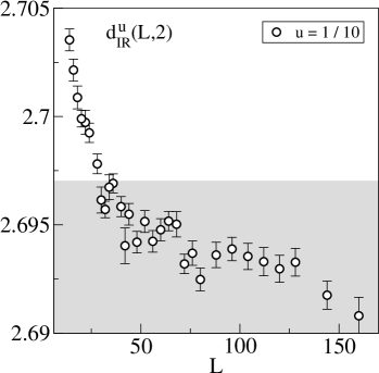
Figure 3: Function $d_{\scriptscriptstyle{\text{\rm IR}}}^{u}(L)$ is decreasing for $u=1/10$, constraining $d_{\scriptscriptstyle{\text{\rm IR}}}$ to be below the onset of shaded region.

PROPOSED RESOLUTION

Below we present additional features of our data which, together with the above, point to coherent explanation of observed inconsistencies between the mMF prediction and numerical results for $d_{\scriptscriptstyle{\text{\rm IR}}}$.

1. Upper Constraint. Construction of effective counting dimension ($d_{\scriptscriptstyle{\text{\rm IR}}}$ here) Alexandru and Horváth (2021); Horváth et al. (2022) from effective number theory Horváth and Mendris (2020) includes identifying counting schemes that lead to consistent effective supports. These schemes, represented by functions of $P=(p_{1},\ldots,p_{N})$, are specified by Horváth et al. (2022)

$$\mathscr{N}_{(u)}[P]=\sum_{i=1}^{N}\min\,\Bigl{\{}\frac{Np_{i}}{u},1\Bigr{\}}\quad,\quad 0<u\leq 1\;$$ (14)

Note that $\mathscr{N}_{(1)}\!=\!\mathscr{N}_{\star}$. Uniqueness of $d_{\scriptscriptstyle{\text{\rm IR}}}$, proved in Horváth et al. (2022), means that the associated $d_{\scriptscriptstyle{\text{\rm IR}}}^{u}(L)$ satisfy

$$\lim_{L\to\infty}d_{\scriptscriptstyle{\text{\rm IR}}}^{u}(L)=d_{\scriptscriptstyle{\text{\rm IR}}}\quad,\quad\forall\;u\;$$ (15)

This property can be used to constrain $d_{\scriptscriptstyle{\text{\rm IR}}}$ based on robust behavior of data rather than fitting. Indeed, from $\mathscr{N}_{(u_{1})}[P]\geq\mathscr{N}_{(u_{2})}[P]$ for all $u_{1}\!<\!u_{2}$ and $P$, it follows that $d_{\scriptscriptstyle{\text{\rm IR}}}^{u_{1}}(L)\geq d_{\scriptscriptstyle{\text{\rm IR}}}^{u_{2}}(L)$ for sufficiently large $L$. This implied order was already seen even on very small Anderson systems Horváth et al. (2022). Hence, although $d_{\scriptscriptstyle{\text{\rm IR}}}(L)$ approaches $d_{\scriptscriptstyle{\text{\rm IR}}}$ from below, $d_{\scriptscriptstyle{\text{\rm IR}}}^{u}(L)$ may descend from above for sufficiently small $u$, and majorize the value of the limit. In Fig. 3 we show this for $u\!=\!1/10$ which is in a decreasing regime. The observed trend suggests a (conservative) upper restriction

$$d_{\scriptscriptstyle{\text{\rm IR}}}<2.697\ll 2.733(3)\;$$ (16)

where “$\ll$” refers to differences relevant in this problem.

2. The Log. At the heart of arguments in Burmistrov (2022) is the claim that the leading power governing $\langle\mathscr{N}_{\star}\rangle_{L}$ has a logarithmic prefactor, i.e. $\langle\mathscr{N}_{\star}\rangle_{L}\propto\ln(L)^{\gamma}L^{d_{\scriptscriptstyle{\text{\rm IR}}}}$ for $L\!\to\!\infty$. While the strict mMF prediction $\gamma\!=\!-1/2$ is not visible in the data (see our first response), it is prudent to inquire about the possibility of other non-zero value since it is allowed on general grounds. To that effect, we fitted our data over the entire available range ($6\leq L\leq 160$), and obtained a very good description ($\chi^{2}/\text{dof}\!=\!1.0$) with parameters

$$\text{log:}\quad\;\;d_{\scriptscriptstyle{\text{\rm IR}}}=2.704(1)\quad\;,\quad\;\gamma=-0.202(2)\;\;$$ (17)

While this nominally suggests that the obtained $\gamma$ and $d_{\scriptscriptstyle{\text{\rm IR}}}$ characterize true asymptotics, the tension of the latter with constraint (16) and Fig. 3 makes it somewhat dubious. Also, logs are known for their capacity to subsume other behaviors. Needless to say, description (17) also contradicts mMF predictions.

3. The Powers. However, barring standard mMF expectations, there is no fundamental reason for multiplicative log in the leading term. In fact, we obtained a high-quality fit ($\chi^{2}/\text{dof}\!=\!1.0$) of our extended $\mathscr{N}_{\star}$ data over the full range ($6\leq L\leq 160$) for a 2-power description $aL^{d_{\scriptscriptstyle{\text{\rm IR}}}}+bL^{d_{m}}$ with

$$\text{powers:}\quad\;\;d_{\scriptscriptstyle{\text{\rm IR}}}=2.673(2)\quad\;,\quad\;d_{m}=1.998(29)\;\;$$ (18)

Note that there is no tension of this log-free description with constraint (16) and Fig. 3. While this already provides rationale for adopting scenario (18) over (17), the logs are deeply rooted in mMF practice and their absence needs an explanation in multifractal terms.

4. The Resolution. Described inconsistencies between mMF predictions and data have two principal manifestations, both pointing to the same underlying cause. First, they suggest in distinct ways that $d_{\scriptscriptstyle{\text{\rm IR}}}\!\ll\!f_{m}(3)\!=\!2.733(3)$. At the same time, relation (7) clearly shows that $f(\alpha)$ is connected to $d_{\scriptscriptstyle{\text{\rm IR}}}$, likely via $d_{\scriptscriptstyle{\text{\rm IR}}}=f(3)$ i.e. in the way proposed in Burmistrov (2022) but with $f_{m}$ replaced by $f$. This suggests that the ensuing tension is connected to possible differences between these characteristics.

Secondly, our numerical analysis raised the possibility that multiplicative log may not accompany the leading power in $\langle\mathscr{N}_{\star}\rangle_{L}$. At the same time, the “log paradigm” in mMF stems in fact from its “shape paradigm”. Indeed, $f_{m}(\alpha)$ is expected to be a smooth concave function with special points, most notably a single $\alpha_{1}$ satisfying $f_{m}(\alpha_{1})\!=\!\alpha_{1}$, and a unique $\alpha_{0}$ satisfying $f_{m}(\alpha_{0})\!=\!3$ and $f_{m}^{\prime}(\alpha_{0})\!=\!0$. In this setting, the relevant $\alpha$-integrals are dominated by one spectral point and multiplicative logs in leading powers are almost inevitable indeed. This again steers us in the direction that $f(\alpha)$, which does not have such restrictions, may be different from $f_{m}(\alpha)$ in a manner that avoids the leading multiplicative log.

Following the above leads, we propose that at Anderson criticality in 3D, functions $f_{m}(\alpha)$ and $f(\alpha)$ are not identically equal to each other, namely

$$\text{conjecture:}\quad f\neq f_{m}\quad,\quad\ d_{\scriptscriptstyle{\text{\rm IR}}}=f(3)<f_{m}(3)\;\;$$ (19)

One possible realization commensurate with existing evidence is the presence of a segment in $f(\alpha)$ represented by the red solid line in Fig. 4. In particular, $f(\alpha)=f(3)$ for $\alpha_{+}\leq\alpha\leq 3$ and $f(\alpha)=\alpha$ for $\alpha_{-}\leq\alpha\leq\alpha_{+}$. The horizontal segment is key for the present argument because it can generate pure power $aL^{f(3)}=aL^{d_{\scriptscriptstyle{\text{\rm IR}}}}$ upon evaluating its contribution to (4). Indeed, the integral determining $a$, namely $\int_{\alpha_{+}}^{3}v(\alpha,L)d\alpha$, cannot diverge for $L\to\infty$ and our numerical experiments show that it is increasing and thus finite. While details will be given elsewhere, the horizontal segment offers a robust mechanism for generating a log-free leading power in $f(\alpha)$. Note that the difference that sparked this discussion is one between the red dot and the black data point at $\alpha=3$ in Fig. 4.

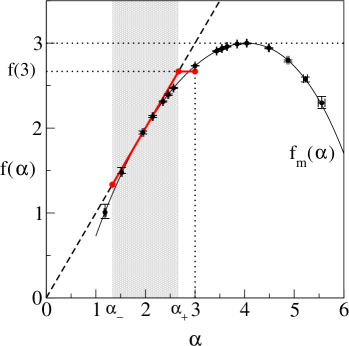
Figure 4: Possible realization of $f(\alpha)\neq f_{m}(\alpha)$ is via $f(\alpha)$ featuring the red solid segment. The $f_{m}(\alpha)$, shown to guide the eye, is from Ref. Ujfalusi and Varga (2015).

The nominal purpose of the linear $(\alpha_{-},\alpha_{+})$ segment is to ensure that there is a gap between $f(3)=d_{\scriptscriptstyle{\text{\rm IR}}}$ and the subleading behavior, which is needed to explain the remarkably accurate 2-power description (18) of the data. Indeed, one can easily check that, for slowly varying (in $\alpha$) $v(\alpha,L)$, the integral (4) only generates powers of $f(3)=\alpha_{+}$ and $\alpha_{-}$, with prefactors vanishing as $1/\sqrt{L}$. This is both harmless to the leading term and creates a gap.

The attractive feature of the above scenario is that it is also consistent with the recent multidimensional analysis Horváth and Markobs (2022b) which suggests that there is a finite probability to find dimensions in any part of interval $[d_{\scriptstyle{\text{\rm min}}},d_{\scriptstyle{\text{\rm max}}}]\approx[4/3,8/3]$. This contradicts the usual mMF paradigm that, in the thermodynamic limit, only information dimension $f_{m}(\alpha_{1})$ is found. The corresponding difference is exactly the one between $f_{m}(\alpha)$ only having a single point satisfying $f_{m}(\alpha)\!=\!\alpha$, and the above proposal that $f(\alpha)\!=\!\alpha$ on the entire interval $[\alpha_{-},\alpha_{+}]$. In fact, the connection is direct and $[d_{\scriptstyle{\text{\rm min}}},d_{\scriptstyle{\text{\rm max}}}]\equiv[\alpha_{-},\alpha_{+}]$.

Another surprising support for the above proposal comes from the details of our findings in Ref. Horváth and Markobs (2022b). Indeed, given that $\alpha_{-}\!=\!d_{\scriptstyle{\text{\rm min}}}\!\approx\!4/3$, it may seem surprising that the 2-power description (18) involves a subleading $d_{m}\!\approx\!2$. However, this is in fact expected given the results of multidimensional analysis Horváth and Markobs (2022b), which concluded that dimension $d_{m}\!\approx\!2$ is discrete. Its special status is not captured by $f(\alpha)$ since it has a $\delta$-function prefactor. But its role is of course crucial for capturing the small $L$ behavior which is exactly why 2-power description works so well. In fact, the closeness of fitted value to $d_{m}\!=\!2$ independently supports the proposition of Horváth and Markobs (2022b) that $d_{m}$ may be an integer.

We finally wish to emphasize three points.

(a) By performing an extensive numerical analysis, we have shown that, even in the full form (2) of Ref. Burmistrov (2022), mMF is unable to describe data for $d_{\scriptscriptstyle{\text{\rm IR}}}(L)$. Observing the practice of not blaming accurate data for refusing to follow the theory but the other way around, we are led to conclude that the mMF prediction $d_{\scriptscriptstyle{\text{\rm IR}}}\!=\!f_{m}(3)\!=\!2.733(3)$ is unreliable. As shown from several different angles, the extent of the tension is such that the conclusions on $d_{\scriptscriptstyle{\text{\rm IR}}}$ based on mMF, at least in the form suggested by Burmistrov (2022), cannot be used to judge the correctness of our conclusions (m1) and (m2) Horváth and Markobs (2022a).

(b) Our analysis showed that the observed discrepancies have to be interpreted, in fact, as those between predictions of MF and mMF. This observation is crucial for the proposed resolution $f\!\neq\!f_{m}$ (19). In that regard, the contribution of Comment Burmistrov (2022) is very valuable. While the debate regarding $d_{\scriptscriptstyle{\text{\rm IR}}}$ and $f_{m}(3)$ may continue, it already focused the attention on the possibility to evaluate $f(\alpha)$ directly. This may not be unrealistic since the computer power has improved greatly from early days of MF when similar calculations were attempted. Nevertheless, computing $f(\alpha)$ is certainly not an efficient way to evaluate a basic geometric characteristic of a multifractal such as $d_{\scriptscriptstyle{\text{\rm IR}}}$.

(c) Our proposal that $f(\alpha)$ features a finite $f(\alpha)\!=\!\alpha$ segment is equivalent to the conclusion of Ref. Horváth and Markobs (2022b) that Anderson critical states are not only multifractal, but also multidimensional. This possibility entails an important geometric consequence, namely that critical Anderson states may not be self-similar. Indeed, in standard UV settings, self-similar multifractals have to obey the shape paradigm Falconer (2014). If multidimensionality is indeed realized, this would bring new and interesting geometric detail into the long story of Anderson transitions, and MF approach may play a very relevant corroborating role.