Loss Adapted Plasticity in Deep Neural Networks to Learn from Data with Unreliable Sources

Abstract

When data is streaming from multiple sources, conventional training methods update model weights often assuming the same level of reliability for each source; that is: a model does not consider data quality of each source during training. In many applications, sources can have varied levels of noise or corruption that has negative effects on the learning of a robust deep learning model. A key issue is that the quality of data or labels for individual sources is often not available during training and could vary over time. Our solution to this problem is to consider the mistakes made while training on data originating from sources and utilise this to create a perceived data quality for each source. This paper demonstrates a straight-forward and novel technique that can be applied to any gradient descent optimiser: Update model weights as a function of the perceived reliability of data sources within a wider data set. The algorithm controls the plasticity of a given model to weight updates based on the history of losses from individual data sources. We show that applying this technique can significantly improve model performance when trained on a mixture of reliable and unreliable data sources, and maintain performance when models are trained on data sources that are all considered reliable. All code to reproduce this work’s experiments and implement the algorithm in the reader’s own models is made available.

I Introduction

In many machine learning applications, data is recorded by multiple sources, which are merged together to form a dataset. For example, in healthcare monitoring applications, data from multiple recording devices or sites are often pooled together into a single dataset [1, 2]. However, within a dataset, data sources may not provide the same level of data quality and could include noisy observations, incorrect labelling or missing values. In general, machine learning models are trained using multi-source datasets, often without consideration of the reliability of the underlying data sources. This can have detrimental effects on the performance and robustness of these models. We propose a technique that can be implemented alongside any gradient descent optimisation algorithm, which automatically distinguishes between reliable and unreliable data sources over time; mimicking the way children learn from multiple information sources, and controls a model’s plasticity (the models readiness to learn) to those sources. Our solution proposes that model weight plasticity should be a function of the perceived reliability of data sources. To achieve this, our new approach maintains a distribution of weights over the set of data sources, which in turn are used to control the back-propagation of gradient updates to the model. Within this work, we focus on the data corruption of observations and labels, and do not consider missing data directly; even so, some of our experimental contexts could be considered special cases of learning with missing data, making our algorithm potentially useful in this context too. Future work could also explore the use of this algorithm in a continual learning setting, in which data is streaming online from multiple data sources. It could also be used in settings in which models are required to learn new tasks without forgetting previous tasks, such as the case in Li et al. [3].

In neuroscience, plasticity in the brain allows the biological neural networks to change and reorganise in response to different stimuli. In this work we propose a plasticity technique which allows the model to adapt and respond to changes in the reliability of the information sources. This is done via measuring and evaluating the loss of the model in response to each source of information (i.e stimuli). We therefore refer to this technique as Loss Adapted Plasticity.

The main contribution of this work include:

• A neuroscience inspired technique to improve the performance of any deep learning model when learning from data with unreliable sources.

• Provides a mathematical foundation with hyperparameter optimisation to identify unreliable sources in datasets originating from multiple providers with unknown reliability.

• Evaluates the training algorithm and demonstrates the applicability of the solution to gradient based training methods in a wide variety of contexts.

The paper discusses the related work, especially closely related methods in Federated Learning, before presenting the main inspirations behind the proposed research. Next, we present our solution, titled Loss Adapted Plasticity (LAP), as well as the baseline methods that we will use to evaluate its performance. We will then discuss the results and some immediate questions that arise about the technique’s practical use. Finally, we will mention the current limitations before concluding the research and discussing future work.

All code and experiments are available to study and reproduce, and an implementation of the LAP training methods written for Pytorch [4] are available , allowing for users to incorporate this research into their own models easily.

II Related Work

Children are effective at learning from testimony and do not accept to learn from any speaker, but rather learn from a speaker that they consider trustworthy and knowledgeable [5]. Children will then begin to give greater weight to trustworthy sources as a result of their experiences, learning less from perceived untrustworthy sources [6]. It is this natural dynamic weighting of source trust that we wish to capture in our proposed algorithm.

In machine learning, learning from multi-sourced data (multiple devices, deployment sites, or manually labelled resources) is often done without much regard for each source’s data quality. However, when sources have reduced data quality, training methods should recognise when not to learn or with greater caution to produce the most optimal model [7]. Frequent approaches to this challenge utilise methods that cope with noisy data, noisy labels, or both, as well as federated learning models. Song et al. [7] provides a survey of techniques used to deal with noisy labels, in particular. A common method is to apply pre-processing or filtering techniques before training; during which labels or data suspected of being unreliable are removed or rectified. Several other methods consider changing the architectures of models to ensure they are robust to noise in labels [8, 9], limiting them to classification problems, and do not address the problem of noisy observations. Other work focuses on the task of dealing with noisy labels through the use of regularisation, robust loss design, and sample selection [7]. Robust loss design can involve loss re-weighting; in which loss values and data points are weighted based on, for example, meta-learning methods [10] or using exponential gradient re-weighting [11]. However, these works treat data points independently from the sources that they originate from. Majidi et al. [11] specifically, store weights for each data point, limiting the method to offline training only. This differs from our proposed technique, in which weights are stored per source, meaning new data from existing sources can be weighted immediately, allowing for its use in continual learning. This also reduces computational and memory expenses.

Federated Learning allows for training models on data from multiple sources whilst respecting each source’s privacy. The server trains a global model based on local updates of models on each source device, eliminating the requirement for a centralised server to store and handle data [12]. When data sources are unreliable (i.e., client data is corrupted or potentially malicious), federated learning algorithms may fail [13], as local model updates can have negative effects on the global model. Jebreel et al. [14] and Stripelis et al. [15] discuss solutions to situations in which unreliable data is malicious (i.e., in adversarial attacks), but do not consider noisy observations from benevolent sources. To tackle the issue of varied data quality in client data, Li et al. [16] proposed a novel federated learning approach called Auto-weighted Robust Federated Learning (ARFL) which learns the global model and the weights of local updates simultaneously. We will refer to this model as FED ARFL to emphasise its grounding in Federated Learning. The weighted sum of empirical risk of clients’ loss is minimised with a regularisation parameter, where the weights are distributed by comparing each client’s empirical risk to the average empirical risk of the best $k$ clients. The contribution to weight updates of the clients with higher losses are minimised in respect to the updates from other clients; allowing the global model to learn more from clients that achieve lower losses. FED ARFL will serve as a baseline model in our study as it is the closest research in the literature to the setting that we investigate. However, in our testing, we allow for the transfer of data to the server, since we are not concerned with this constraint.

III Preliminaries and Motivation

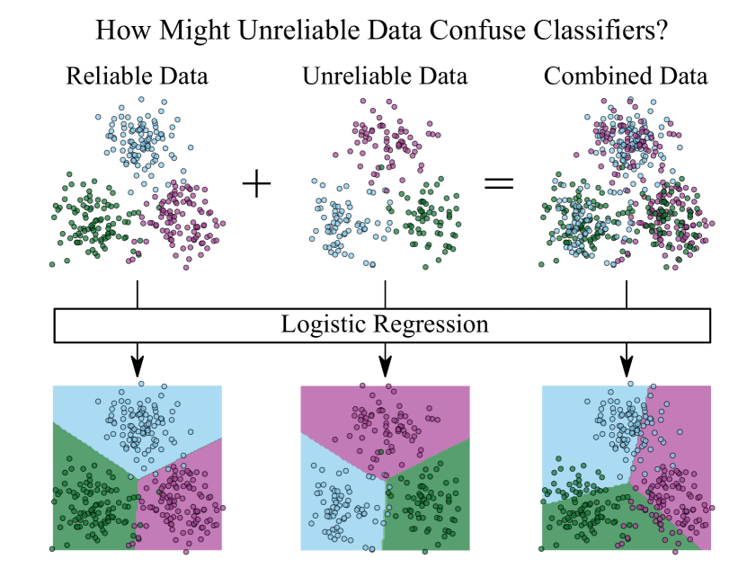
Figure 1: Example of distribution and logistic regression model applied to a database made up of 3 classes. The three graphs at the bottom show the areas of the plane for which a Logistic Regression model predicted the class with their corresponding colour. The bottom left one shows the boundaries after being trained on the reliable data sources only; the one in the centre shows the boundaries when trained on the unreliable sources; and the one on the right shows the boundaries for a combination of the two, overlaid on the reliable data.

When designing predictive models for analysing multi-source/multi-site data, it is common to treat data sources as having equal reliability [1, 2]. Predictive models trained on unreliable data could lead to reduced performance and potentially, unforeseen consequences when deployed in production.

Integrating multi-source data into single datasets before performing model training and testing could result in the reduction of model performance on reliable data. Figure 1 shows the decision boundaries of a logistic regression model trained on data from a reliable source, an unreliable source, and both. In this experiment, $60\%$ and $40\%$ of the data is chosen to be reliable and unreliable respectively. We see that unreliable data sources can contaminate the training data and significantly reduce a model’s performance.

These challenges motivate us to design an intentionally straight-forward technique that can be applied to all gradient descent optimisers, allowing for wide applicability and ease-of-use. The objective is to control the influence of unreliable data sources on the weight updates of a deep neural network and satisfy the following criteria: 1: Identify and reduce the level of trust of unreliable data sources, without compromising learning on reliable data. 2: Update the level of previously unreliable data sources, if data from these sources becomes reliable again. 3: Easily implementable alongside existing models. And 4: Require limited additional compute expense. These requirements would make the technique suitable in diverse contexts, applicable to a variety of deep learning architectures, and allow for easy adoption.

III-A Unreliable Data Sources

As discussed in Section III, unreliable data sources can be introduced in a multitude of ways, affecting both the independent and dependent variables of data. To create unreliable data for controlled and verifiable experiments in this paper, we apply synthetic corruption techniques summarised in Table I. In line with Li et al. [16], we apply label flipping, label shuffling and the addition of Gaussian noise to inputs. Additionally, we choose random labels, replace data with noise and shuffle chunks of the input data to further evaluate the proposed algorithm.

To implement the corruption, data is split into mutually exclusive sources of data points, before a number of these are chosen to be unreliable and corrupted. For each experiment, a single corruption technique is used for all unreliable sources.

TABLE I: Methods used to produce unreliable data sources. *Techniques employed in Li et al. [16].

Corruption Type	Description of Corruption Applied
Original Data	No corruption is applied to the data.
Chunk Shuffle	Split data into distinct chunks and shuffle. This is only done on the first and/or second axis of a given input.
Random Label	Randomly assign a new label to an input from the same domain.
Batch Label Shuffle*	For a given batch of input data, randomly shuffle the labels.
Batch Label Flip*	For a given batch of data, assign all inputs in this batch a label randomly chosen from the batch.
Added Gaussian Noise*	Add Gaussian noise to theinputs, with mean $=0$ and standard deviation $=1$.
Replace with Gaussian Noise	Replace inputs with Gaussian noise, with mean $=0$ and standard deviation $=1$. This can be considered a special case of sources with missing data.

III-B Loss Adapted Plasticity

To learn from data sources with mixed reliability, we propose a technique able to discern the reliable from the unreliable sources, based on the history of losses incurred by a model during training. When a model frequently produces a loss on a given source that is significantly larger than the losses on other sources, the model will become less plastic when updating its weights to that source. We intentionally design this to be straight-forward, to allow for it to be easily implementable alongside all existing gradient descent optimised machine learning models.

We start by assuming that losses generated by sources over a relatively small number of steps follow a normal distribution (discussed in Appendix D). Given a set of sources $S$, a history of losses for each source $\{L_{s}^{t}\}_{s\in S}^{\tau-h+1,\tau}$ (with $h$ denoting the history length and $\tau$ denoting the current step), a distrust level for each source $\{R_{s}\}_{s\in S}$ (in which $R_{\zeta}\in[0,+\infty)$, and a larger value corresponds to a higher level of distrust in $\zeta$), the updated distrust, $R_{\zeta}$ at time step $\tau$ on source $\zeta$ is calculated using the following process:

Calculate the weighted average, $\mu_{s\neq\zeta}$ and standard deviation, $\sigma_{s\neq\zeta}$ of the loss history over all sources and time-steps cached, $[\tau-h+1,\tau]$, excluding the source $\zeta$ currently being updated, and with weights $=\{1/(1+R_{s})\}_{s\neq\zeta\in S}$. This weighting forces sources that are distrusted more, to have less of an influence on the mean and standard deviation of all source losses. The formulas are as follows:

$$\begin{array}[]{c}\mu_{s\neq\zeta}=\frac{\sum_{s\neq\zeta}\sum_{t=\tau-h+1}^{\tau}\frac{1}{1+R_{s}}L_{s}^{t}}{\sum_{s\neq\zeta}\frac{1}{1+R_{s}}}\\ \\ \sigma_{s\neq\zeta}=\sqrt{\frac{\sum_{s\neq\zeta}\sum_{t=\tau-h+1}^{\tau}\frac{1}{1+R_{s}}\times(L_{s}^{t}-\mu)^{2}}{\sum_{s\neq\zeta}\frac{1}{1+R_{s}}}}\end{array}$$ (1)

Then, we calculate the mean loss from the history of the current source, $\mu_{\zeta}$:

$$\mu_{\zeta}=\frac{\sum_{t=\tau-h+1}^{\tau}L_{\zeta}^{t}}{h}$$ (2)

And use $\mu_{\zeta}$, $\mu_{s\neq\zeta}$, and $\sigma_{s\neq\zeta}$ in the following to update the current source’s distrust level, $R_{\zeta}$:

$$R_{\zeta}=\begin{cases}-1&\mu_{\zeta}<\mu_{s\neq\zeta}+\lambda\sigma_{s\neq\zeta}\\ +1&otherwise\end{cases}$$ (3)

Where $\lambda$ is defined as the leniency parameter; used to control the probability that a source producing reliable data is considered less trustworthy. $R_{\zeta}$ can be interpreted as how unreliable a source is considered; the larger the value, the less reliable a source is considered, and the less plastic the model would be to updates based on source $\zeta$. If $R_{\zeta}<0$ after an update, its value is modified to $0$, to ensure that sources that are deemed reliable at the start can be considered unreliable without delay. Model plasticity is controlled through the scaling of gradients in a given gradient descent optimiser. Each back-propagation gradient $g$ is scaled using:

$$\hat{g}=(1-d_{\zeta})g,~{}~{}~{}d_{\zeta}=\tanh^{2}(\delta R_{\zeta})$$ (4)

Here, $\hat{g}$ represents the updated gradients after the gradients $g$ are depressed by the scalar $1-d_{\zeta}$, in which $\delta$ corresponds to the discrete step size (referred to as the depression strength) used to control the rate of change in depression applied. For two sources that are reliable and unreliable respectively, say $\zeta_{r}$ and $\zeta_{u}$, we expect that $d_{\zeta_{r}}<d_{\zeta_{u}}$. This would correspond to less plasticity in the weight updates for a source that is unreliable compared to a source that is producing reliable data. Since $0\leq d_{\zeta}<1$, the gradients are only ever reduced or maintained by this process.

Using this technique, we introduce two main hyper-parameters, namely the leniency ($\lambda$) and the depression strength ($\delta$), which control the criteria for increasing $R_{\zeta}$ and the rate of change of the depression respectively.

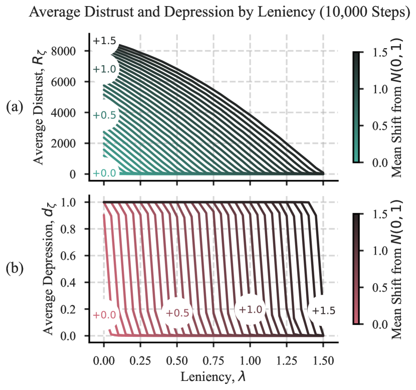
Figure 2: a: $100$ random walkers produced values sampled from the Normal distribution with mean equal to the hue of the figures and standard deviation $1$. Each time that value was more than the leniency, $\lambda$ given by the $x$ axis, the walker increased $R_{\zeta}$ by $+1$, otherwise, it decreased $R_{\zeta}$ by $-1$ as in Equation 3. This step was completed $10,000$ times, to produce the figure. A larger $R_{\zeta}$ represents a higher level of distrust. b: The average depression calculated using $R_{\zeta}$ from each of the walkers in Figure a. A larger value on the $y$ axis ($d_{\zeta}$) represents a lower level of weight plasticity. Both of these figures show that if the loss values are far from the standardised Normal distribution, then the larger the leniency value, the more a model’s weights will be plastic to those weight updates, and shows the specific distrust and depression values that you might expect.

Figure 2 shows how the distrust level and depression can be affected by the leniency parameter, assuming that losses generated by sources form a normal distribution. For example, the loss distribution on reliable data is given mean $=0$ and standard deviation $=1$ and each line represents a source that is producing losses with a mean given by the hue (or the labelled value), and a standard deviation $=1$. The values of distrust and depression are then calculated by taking the average of $100$ walkers (imitating source losses), moving under Equation 3, sampling values from the same distribution for $10,000$ steps. The larger the shift in mean, the more unreliable a source is considered (given by larger values in $R_{\zeta}$ - Figure 2a) for a given leniency, and the less plastic the weights will be to updates on this source (given by a higher value in $d_{\zeta}$ - Figure 2b). The leniency value allows us to control the mean value of loss distributions for which the technique should depress gradient updates. It also allows us to calculate the probability of a source producing reliable data having its level of distrust increased.

The depression strength parameter, $\delta$, controls the rate of change of the depression. Too small a $\delta$ value and the unreliable sources may have a significant negative effect on the training of a model, however, too large a value and gradient updates from reliable sources may be incorrectly depressed in early training. From our experiments, we found it helpful to split the depression parameter into $\delta_{s}=\delta\times 0.005$. Using $\delta_{s}$ allowed for greater control over the parameter and meant that when $R_{\zeta}$ is on the order of $1000$, the value of $d_{\zeta}$ is close to $0$.

Because of the connection of our algorithm to loss values, and the goal of adapting model plasticity, we refer to this technique as Loss Adapted Plasticity (or LAP). The code has been implemented in Pytorch 1.10 [4] for both Stochastic Gradient Descent and the Adam algorithm [17], but can be easily extended to any other gradient descent optimiser. For further notes on the practical use of LAP, see Section V.

IV Experiments and Results

To investigate the performance of the Loss Adapted Plasticity (LAP) algorithm, we employ image datasets and synthetically produce unreliable sources before evaluating models trained using LAP and in the standard way. In addition, we compare our technique against FED ARFL; the training algorithm presented by Li et al. [16]. We will evaluate all models on reliable, uncorrupted data. We choose to focus on synthetic experiments to ensure that our experiments are reproducible and accessible. Additionally, we test our algorithm on two real-world datasets; a healthcare dataset and a human labelled imaging dataset. The results on the former are presented alongside the results on the synthetic data and the results on the latter are presented in Appendix C-A.

IV-A Datasets

In order to evaluate the proposed techniques, four datasets are employed: CIFAR-10 and CIFAR-100 [18], Fashion-MNIST (F-MNIST) [19], and an electrocardiograph (ECG) dataset: PTB-XL [20]. CIFAR-10 and CIFAR-100 are datasets made up of $60,000$ RGB images of size $32\times 32$ divided into 10 and 100 classes, with $6,000$ and $600$ images per class respectively. The task in this dataset is to predict the correct class of a given image. F-MNIST is made up of $70,000$ greyscale images of clothes of size $28\times 28$ divided into 10 classes with $7,000$ images per class, which was flattened into datapoints with 784 features. The task of this dataset is to predict the correct class of a given image. Finally, PTB-XL consists of $21,837$ ECG recordings, sampled at $100$Hz, from $18,885$ patients, labelled by $12$ nurses. The task of this dataset is to predict whether a patient has a normal ECG reading or not. CIFAR-10, CIFAR-100, and F-MNIST are managed under the MIT License, whilst PTB-XL is made available with the Creative Commons Attribution 4.0 International Public License .

CIFAR-10, CIFAR-100, and F-MNIST are chosen as they are three of the most notable datasets that are employed for object classification. Moreover, Li et al. [16] uses CIFAR-10 to benchmark their model, aligning our evaluation with the Federated Learning literature. PTB-XL is chosen to illustrate the performance of our proposed training technique on a real-world healthcare dataset, that contains time-series observations.

Before any manipulation of the dataset took place, the recommended test set from each of the datasets are extracted and removed from the training data, allowing our performance measurements to be accurate.

To implement the notion of reliable and unreliable data sources, data was split into $10$ distinct groups, with datapoints randomly assigned to each. For CIFAR-10 and CIFAR-100, $4$ and $2$ of these sources were chosen to be unreliable respectively, whilst for F-MNIST $6$ were chosen to be unreliable. Since PTB-XL was labelled by $12$ nurses, this is chosen as the dividing attribute when splitting the data into sources. However, since the data was clinically validated and is of high quality, synthetic corruption of the data is required to be able to evaluate the proposed techniques. We therefore choose $4$ sources to be corrupt, and use the Gaussian distribution to add noise to $50\%$ of these sources’ ECG observations (simulating electromagnetic interference [21]). The data sources are then upsampled so that each source contains the same number of observations.

For CIFAR-10, CIFAR-100, and F-MNIST unreliable data was corrupted using the techniques discussed in Section III-A, and remained corrupted for the full duration of training.

Data from each source is batched in sizes of $128$ for CIFAR-10 and CIFAR-100, sizes of $200$ for F-MNIST, and $64$ for PTB-XL. Each batch contains data from a single source to ensure that weight updates corresponded to single sources, allowing us to control plasticity of weights determined by the data source. Each dataset was split further into a training and validation set with ratio $3:1$ to tune hyper-parameters.

IV-B Models

After the data is loaded into batches, and reliable and unreliable data sources are chosen, the training process begins. Multiple models and training procedures are used to evaluate the performance of Loss Adapted Plasticity (LAP), which are detailed below:

1. CIFAR-10 and CIFAR-100: A convolutional network consisting of $3$ convolutional layers and $2$ fully connected layers is chosen. This model is trained for $25$ epochs, with the Adam algorithm [17], and a learning rate of $0.001$. For FED ARFL global updates were performed $25$ times, in which all clients are trained on data for a single epoch, to keep training consistent across techniques.

2. F-MNIST: A fully connected model is chosen consisting of $3$ layers. The model is trained for $40$ epochs using the Adam algorithm [17], and a learning rate of $0.001$. For FED ARFL global updates were performed $40$ times, in which all clients are trained on data for a single epoch.

3. PTB-XL: A ResNet model consisting of 4 ResNet blocks containing a convolutional layer and $3$ fully connected layers is chosen. This is trained for $40$ epochs using the Adam algorithm [17], and a learning rate of $0.001$.

The full architectures can be explored on the linked code repository. Code for FED ARFL is made available by the authors [16], with an MIT Licence.

IV-C Training

To evaluate the performance of LAP against the baseline models, we test three different training setups:

1. Standard Model: Trained with no knowledge of the sources and whether they are reliable or not.

2. LAP Model: Trained with the knowledge of the source label, but not whether it is reliable or not. Here, we use the LAP extension to Adam with a loss history length of $25$ for CIFAR-10, CIFAR-100 and PTB-XL, and $50$ for F-MNIST, a depression strength of $\delta_{s}=1.0$, and a leniency of $\lambda=0.8$. $\lambda$ and $\delta_{s}$ were chosen using the validation dataset and the analysis in Section III-B. When training on CIFAR-100, we started applying LAP after $250$ gradient update steps, for reasons discussed in Section V-D.

3. FED ARFL [16]: The model as described in Section IV-B, however, each source (or client in the context of Federated Learning) corresponds to a single instance of the corresponding network described in Section IV-B. All other parameters were kept as default in the code made available by the authors [16].

Every experiment is performed $10$ times with different random seeds to ensure the reproducibility and accuracy of results.

V Results and Discussion

We present the results of the experiments and the accuracy of each model, trained on unreliable and reliable data sources, and evaluated on reliable data to show that Loss Adapted Plasticity (LAP) provides a solution to training with data sources of mixed reliability. For an additional experiment on real-world data, please see Appendix C-A.

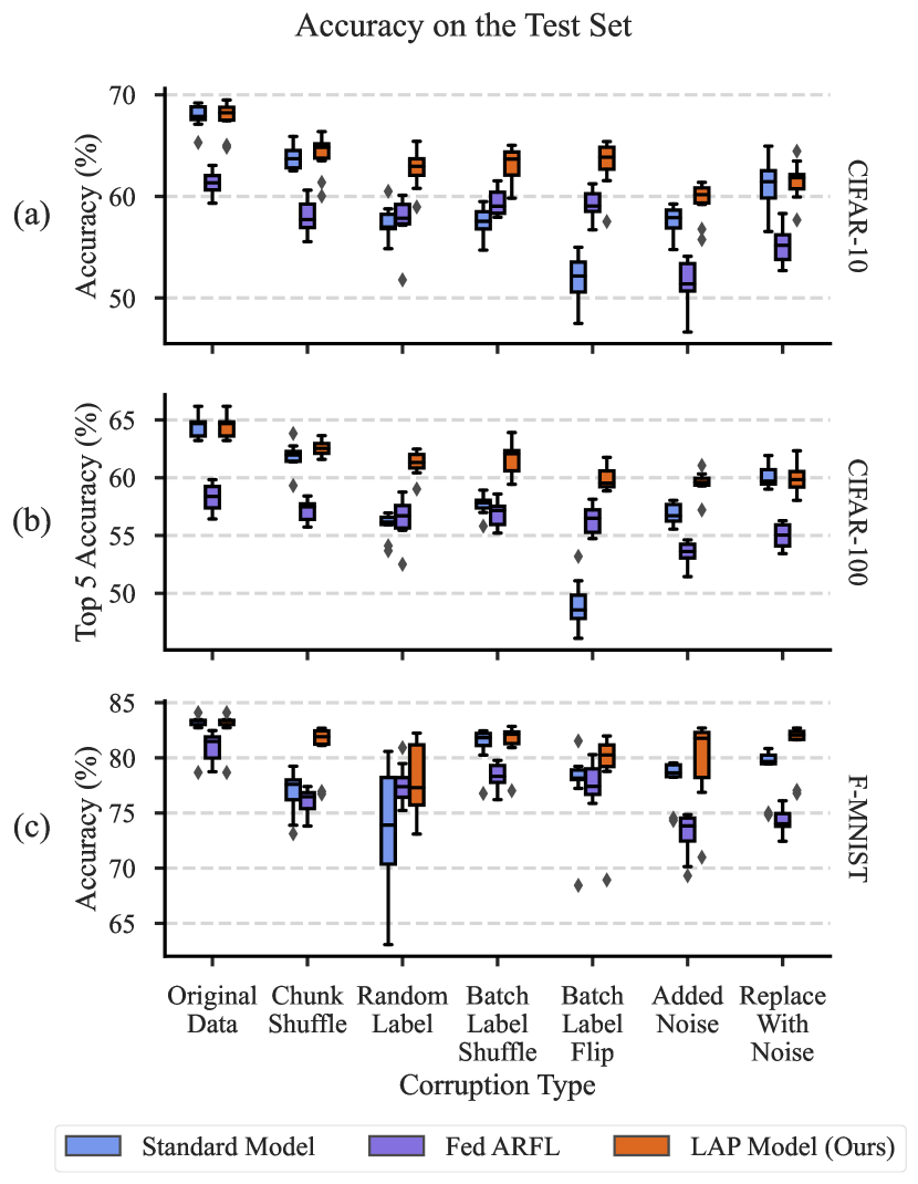
Figure 3: Accuracy when trained on unreliable data and tested on reliable data, with $10$ repeats. a: CIFAR-10; $4$ out of $10$ total sources were corrupted. b: CIFAR-100; $2$ out of $10$ total sources were corrupted. c: F-MNIST; $6$ out of $10$ total sources were corrupted.

Figure 3 shows the results of the models described in Section IV-B, trained on three different imaging tasks, with various corruption techniques. We see that LAP training out-performs both the standard training method, and FED ARFL in all experimental set-ups in which data is corrupted, and matches the performance of the standard model when no corruption is applied.

Figures 3a and 3b show that LAP enabled the models to significantly out-perform both the standard training method and FED ARFL for the CIFAR-10 and CIFAR-100 datasets in which the labels are used to corrupt the source data (random label, label shuffling and batch flip). Here, LAP training also outperforms both of the baseline models when the input data is corrupted, although less significantly. Moreover, when trained on reliable data, both the standard training and LAP training performed similarly, suggesting that LAP is able to boost performance when trained on combinations of reliable and unreliable data, without reducing the performance of models trained on reliable data.

On F-MNIST, the LAP trained model outperforms the standard trained model, and both outperform FED ARFL. Furthermore, Figure 3c shows that the LAP and standard trained model performed equally when trained on data that was reliable.

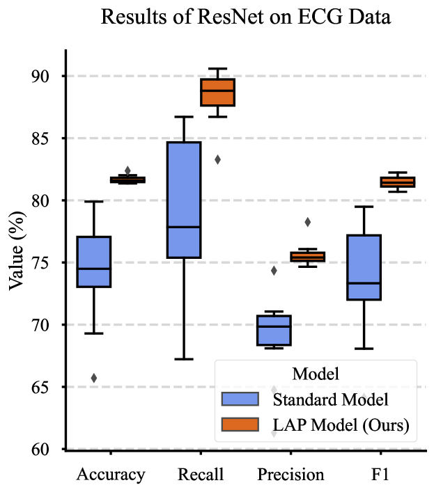
Figure 4: Metrics of performance for a ResNet trained in the standard way and using LAP. The models are evaluated on a test set of an ECG dataset and are tasked with predicting heart abnormalities in the data.

Figure 4 shows the performance of a deep learning model with the ResNet architecture trained in the standard way and using Loss Adapted Plasticity (LAP). In all metrics, our proposed method improves performance of the underlying model and enables a reduction in the variability of the results. This shows experimentally that LAP can have significant effects when applied to real-world data.

Appendix A shows the test results on CIFAR-10 with batch label flipping and the same experimental set-up as in Figure 3a for varying values in the depression strength, leniency, and history length.

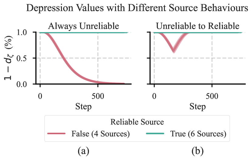
Figure 5: (a) The depression values for each of the sources when training the model using LAP. In total there are $6$ reliable sources and $4$ unreliable sources (corrupted using random labelling), corresponding to the hue of the lines. (b) The depression values for the LAP trained model on CIFAR-10, in which the $4$ sources become reliable after an amount of steps, corresponding to the hue of the lines. In both, the y-axis represents the value of $1-d_{\zeta}$ in Equation 4, implying that a value of $1$ represents no depression applied to the gradient updates for that given batch.

V-A Is Lost Adapted Plasticity Identifying the Correct Sources?

Figure 5a shows the depression applied to the gradient updates ($1-d_{\zeta}$ in Equation 4, Section III-B), for the $10$ data sources during training, on the CIFAR-10 dataset. Here, $4$ of the data sources are unreliable, and the LAP technique is able to correctly identify these, and reduce their gradients.

V-B Does Lost Adapted Plasticity Detect When Unreliable Sources Become Reliable?

Figure 5b, shows the depression applied to the gradients in updates on each of the sources, split by their reliability. Initially, $4$ sources were unreliable, and the LAP technique depressed the gradient updates on these batches, reducing weight plasticity for the corresponding sources. However, once these sources produced reliable data, the technique reduced the amount of depression applied to the gradient updates, and eventually these sources were treated equivalently to reliable sources.

V-C Does Lost Adapted Plasticity Add Extra Compute Time to the Optimisation Process?

The extra computations required in the optimiser to calculate the depression to apply to a single batch of source data is $O(h\times|S|)$, where $S$ is the number of sources and $h$ is the number of losses to cache for each source. This is also the extra memory cost of using LAP. Training on a single NVIDIA RTX 3080 TI, using Pytorch [4] and the Adam [17] implementation, the times to complete the backward pass for a batch size of $128$ on CIFAR-10 (for model and training description, see Section IV-B, and for dataset description see IV-A) are $0.0026\pm 0.0006$s and $0.0088\pm 0.0021$s (mean $\pm$ standard deviation) for the standard training procedure and for LAP training respectively. For the entire forward and backward pass, the computational times are $0.0038\pm 0.0007$s and $0.0098\pm 0.0021$s respectively. In total, this gives the additional computational time for the forward and backward pass per batch of $0.0060\pm 0.0023$s for this experimental set-up.

V-D When To Start Applying Lost Adapted Plasticity

LAP first requires the model to learn which of the sources are producing data from the same distribution and those that are not. Liu et al. [22] and Xia et al. [23] discuss the learning mechanics of deep learning models; models first fit to reliable data before fitting to unreliable data. Therefore LAP training should commence after the initial model warm-up stage to ensure that it correctly identifies the unreliable sources. In some cases, it might take several steps before the model is able to discern between reliable and unreliable sources. An example of the early learning of a model on CIFAR-100 is given in the Appendix B. To control when LAP is applied, we have added a hold-off parameter to our implementation, which corresponds to the number of update steps after loss histories are filled before gradient depression commences.

V-E Current Limitations

When using Loss Adapted Plasticity (LAP), thought should be given to the underlying data and causes of unreliable data sources. Data sources that are producing consistently low quality measurements will be identified and prevented from negatively affecting the learning on the reliable data. Therefore, LAP training minimises the immediate consequences of training a model on data consisting of reliable and unreliable data sources, and for many applications will produce a final model. Moreover, in some contexts, the useful information that LAP training provides about the data sources and their individual perceived reliability will be helpful in itself for improving the quality of a dataset. It should be noted that in some cases users want to learn a model for the unreliable data. An example could be learning a model to monitor electrocardiogram (ECG) recordings in which the dataset consists of readings from different machines at different sites. A practitioner applying LAP can identify data sources that are not perceived to be from the same distribution as others, possibly arising from a calibration issue in one of the machines, and can act accordingly. In this case, the practitioner might take action by replacing the erroneous machine, or by fine-tuning the model on that machine’s data to produce another predictive model. The key point being that with LAP training, a single machine’s data issues will not cause negative effects on the learning of a model for monitoring on all other machines, and any data quality issues can be quickly identified.

VI Ethics Statement

This work presents an algorithm for improving the performance of a model on reliable data, when trained on data stemming from sources that are producing reliable and unreliable data. We see no immediate ethical consequences of our algorithm, and in fact would argue that Loss Adapted Plasticity (LAP) allows the practitioner to understand more about a model’s learning on a dataset made of collective source data, by identifying those data sources that are producing data that differs from the majority distribution whilst improving model predictive performance.

VII Reproducibility Statement

All code is available, and examples of how to implement the algorithm on new models is given. Experimental results are made available and instructions are given for testing the models on new data or with different parameters. Additionally, all data and benchmarks used within this work are publicly available.

Moreover, all figures within this work use colour palettes which are accessible for readers with colour blindness.

VIII Conclusion

In this research, we propose LAP, Loss Adapted Plasticity; as an intentionally straight-forward and novel addition to any gradient descent algorithm used for deep learning that improves model performance on data produced by multiple sources in which some of the sources are unreliable. LAP training also maintains model performance on reliable data and out-performs the benchmarks from the field of Federated Learning (FED ARFL [16]) and current training methods when training on unreliable data. For deep learning applications in which Federated Learning is not required, and data is produced by multiple data sources or at multiple sites, we believe that there is a strong argument for the use of LAP training to control the model updates on reliable data possibly contaminated by unreliable data sources. Future work will explore the use of LAP in a continual learning setting, in which data is streaming online from multiple data sources. It could also be used in settings in which models are required to learn new tasks without forgetting previous tasks, such as the case in Li et al. [3]. Here, LAP may be used to control the model plasticity to data sources producing unreliable data, or data sources that could cause the model to have significant “forgetting” on previously learnt data.

IX Acknowledgements

This study is funded by the UK Dementia Research Institute’s Care Research and Technology Centre funded by Medical Research Council (MRC), Alzheimer’s Research UK, Alzheimer’s Society (grant number: UKDRI–7002), and the Engineering and Physical Sciences Research Council (EPSRC) PROTECT Project (grant number: EP/W031892/1).

Appendix A Parameter Tuning

Figure 6 shows the results of Loss Adapted Plasticity (LAP) training on CIFAR-10 with the model described in IV-B, with batch label flipping applied to $4$ of the $10$ sources. Depression strength, $\delta=1$; leniency, $\lambda=0.8\text{ or }0.4$; and history length, $h=25$ are the most consistent parameter choices across corruption levels for this dataset, but different values might achieve higher performance in other applications.

Figure 6 suggests that depression strength and strictness can have the most significant effect on the performance of the models.

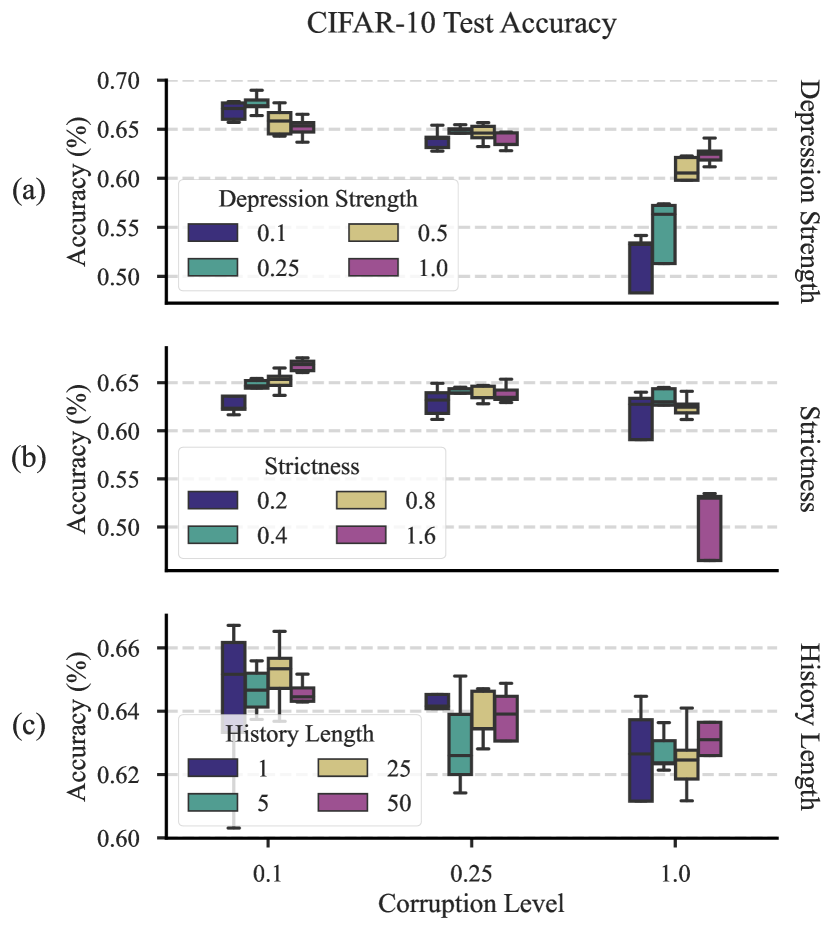
Figure 6: The test performance on CIFAR-10 after being trained on $4$ unreliable sources (corrupted using batch label flipping) at the given corruption level, and $6$ reliable sources. The performance here is shown for various values of each new parameter described in Section III-B. This figure is the result of $5$ runs of each experiment. a: shows the performance for varied depression strength, $\delta$ values; b: for leniency, $\lambda$; and c: for history length, $h$. Unless otherwise stated, depression strength $=1$, leniency $=0.8$, and history length $=25$.

Appendix B Early Learning on CIFAR-100

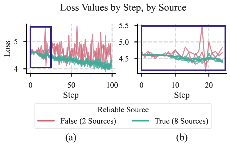
Figure 7: The loss values, plotted per source when training a model in the standard way on CIFAR-100, with $2$ unreliable sources (corrupted using batch label flipping) and $8$ reliable sources. a: Shows these loss values plotted for the first $100$ steps, whilst b: focuses on a section of a, shown by the bounding box, plotted for the first $25$ steps.

Figure 7 shows the loss values, plotted by source when training on CIFAR-100 (model description in Section IV-B), with $2$ unreliable sources and $8$ reliable sources. In this example, the zoomed-in section shows that for the first $\sim 10$ steps, the difference in loss on the reliable and unreliable sources are not clear. For other datasets, this may require more time.

Appendix C Additional Experiments Using Real World Data

To understand the performance of Loss Adapted Plasticity (LAP) on another real world dataset, a human labelled CIFAR-10 dataset was chosen.

C-A Human Labelled CIFAR-10

Figure 8: Accuracy score on the validation set of CIFAR-10N labels, after models were trained on varying amounts of the human labelled (with noisy labels) CIFAR-10N dataset. Results here are shown for varying amounts of unreliable sources and proportions of unreliable labels. For all experiments, there were $10$ sources present in total.

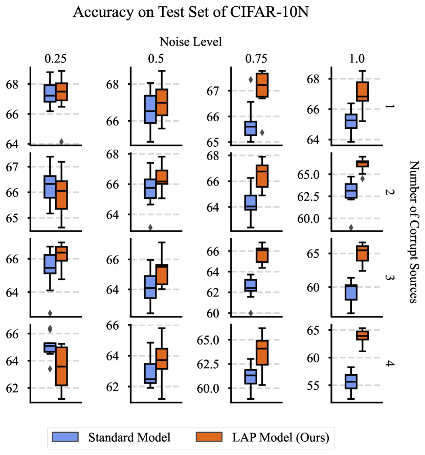
Figure 9: Accuracy score on clean CIFAR-10 labels (performance on the test set) after models were trained on varying amounts of the human labelled (with noisy labels) CIFAR-10N dataset. Results here are shown for varying amounts of unreliable sources and proportions of unreliable labels. For all experiments, there were $10$ sources present in total.

The additional real-world dataset that we have used to better understand the performance of training models with LAP is CIFAR-10N [24] , which contains human labels produced for the CIFAR-10 dataset [18]. This dataset is often used in the literature surrounding learning from noisy labels.

The CIFAR-10N dataset contains the human labels for the training set of CIFAR-10 only, allowing us to evaluate the models on the CIFAR-10 test set. For our experiments, we chose the set of human labels titled “CIFAR-10N Worst”, which contains the human labelling with the highest noise rate, $40.2\%$. We then binned the noisy labels, along with the clean labels into $10$ sources with different noise levels. We chose combinations of $1$, $2$, $3$ and $4$ unreliable sources (containing noisy human labels) and noise levels of $25\%$, $50\%$, $75\%$ and $100\%$, to get a complete understanding of the performance difference between training with and without LAP, on this real-world dataset. The training dataset was split in the ratio $3:1$ to produce a validation set that also contained unreliable data sources. The test set contained only clean labels and corresponded to the standard CIFAR-10 test set.

A convolutional network was tested on this dataset consisting of $3$ convolutional layers and $2$ fully connected layers. This is trained for $25$ epochs, with the Adam algorithm, and a learning rate of $0.001$ and a batch size of $128$. When using the LAP Adam algorithm, a depression strength of $\delta_{s}=1.0$, a leniency of $\lambda=0.8$, and loss history length of $25$ is used.

The results for these training algorithms can be seen in Figure 8 (performance on the validation set) and 9 (performance on the test set). We compare training in the standard way with the LAP training extension. For all but $2$ combinations, it is clear that LAP training outperforms standard training, and reduces the performance gap to the model that is trained on clean labels. This suggests that the proposed algorithm outperforms standard training for a variety of noise levels and number of corrupt sources

We note that LAP outperforms the standard training on both the validation and test sets, suggesting that LAP is better at providing predictions on datasets with sources of mixed reliability, as well as on reliable data.

We also aimed to understand how LAP training would perform in a situation in which the model is significantly under-fitting to the data. To do this, we trained a model with reduced capacity (with $3$ and $6$ channels compared to the previous model of $32$ and $64$ channels in its convolutional layers), on the CIFAR-10N dataset containing $4$ unreliable sources (with noise levels of $100\%$) and $10$ total sources. The testing was performed on reliable data, from the CIFAR-10 dataset. The results of this are shown in Table II, and suggest that LAP trained models also outperform the standard trained model in this context.

TABLE II: Results in an under-fitting context.

Model Name	Accuracy $\pm$ Standard Deviation (%)
Standard Model	$42.85\pm 2.56$
LAP Model (Ours)	$\mathbf{45.97\pm 1.01}$

Appendix D Loss Assumptions

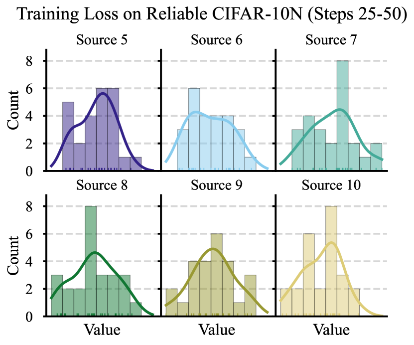
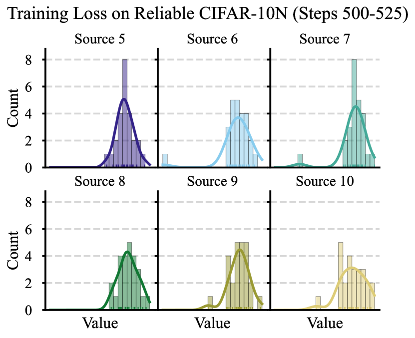
(a) Reliable Sources

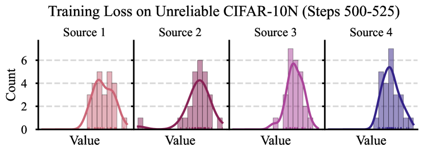
(b) Unreliable Sources

Figure 10: The distribution of loss values over a period of $25$ steps between step $25$ and $50$, and $500$ and $525$, when training a predictive model on the CIFAR-10N dataset. Here, 10(a) show the loss on batches from reliable sources only, binned as described in C-A. Similarly 10(b) shows the same information, except for the unreliable sources. Here, we have $4$ unreliable sources, with noise levels of $100\%$.

One of our assumptions when designing the Loss Adapted Plasticity algorithm is that the loss values are distributed using a normal distribution over a given number of steps. We show in Figure 10 that the loss values approximate a normal distribution at different step values. This allows us to consider the strictness parameter as being related (through the normal distribution) to the probability of a reliable source being incorrectly trusted less, at any given step.

Appendix E Biography Section

Alexander Capstick joined the UK Dementia Research Institute (UKDRI) and Imperial College London as a PhD student in 2021 under the supervision of Payam Barnaghi. He was awarded his MSc in Applied Mathematics at Imperial College London (2020) and BSc in Mathematics at University College London (2019). At present, his research focus is on the use of machine learning models for the extraction of clinical insights from in-home monitoring data and is interested in continual learning and meta-learning. Alex is also interested in building techniques for learning reliable machine learning models from unreliable data.

Francesca Palermo joined the UK Dementia Research Institute (UKDRI) and Imperial College in 2021, as a Research Associate. She received her B.Sc (2014) and M.Sc (2017) in Artificial Intelligence and Robotics from Sapienza University of Rome. She was awarded a Ph.D. (2022) in Electronics Engineering from Queen Mary University of London in the Advanced Robotics lab (ARQ) as a member of the Human Augmentation & Interactive Robotics (HAIR) under the supervision of Dr. Ildar Farkhatdinov and Dr. Stefan Poslad. She is now working in the Care Research & Technology at UKDRI and her research focuses on detecting health related episodes in people living with dementia by applying recurrent deep learning models on personalised data (activity, sleep and physiologycal data).

Payam Barnaghi is Professor and Chair in Machine Intelligence Applied to Medicine in the Department of Brain Sciences at Imperial College London. He is a Co-PI and Programme Lead in the Care Research and Technology Centre at the UK Dementia Research Institute. He is also a visiting Professor in the Visiting Professor at the Great Ormond Street Institute of Child Health at University College London. He is an associate editor of the IEEE Transactions on Big Data and vice-chair of the IEEE SIG on Big Data Intelligent Networking. His research interests include machine learning, Internet of Things, computational neuroscience and healthcare applications.

References

- [1] E. Baro, S. Degoul, R. Beuscart, and E. Chazard, “Toward a literature-driven definition of big data in healthcare,” BioMed research international, vol. 2015, 2015.
- [2] D. Tomar and S. Agarwal, “A survey on data mining approaches for healthcare,” International Journal of Bio-Science and Bio-Technology, vol. 5, no. 5, pp. 241–266, 2013.
- [3] H. Li, P. Barnaghi, S. Enshaeifar, and F. Ganz, “Continual learning using bayesian neural networks,” IEEE Transactions on Neural Networks and Learning Systems, vol. 32, no. 9, pp. 4243–4252, 2021.
- [4] A. Paszke, S. Gross, F. Massa, A. Lerer, J. Bradbury, G. Chanan, T. Killeen, Z. Lin, N. Gimelshein, L. Antiga, A. Desmaison, A. Kopf, E. Yang, Z. DeVito, M. Raison, A. Tejani, S. Chilamkurthy, B. Steiner, L. Fang, J. Bai, and S. Chintala, “Pytorch: An imperative style, high-performance deep learning library,” in Advances in Neural Information Processing Systems 32, H. Wallach, H. Larochelle, A. Beygelzimer, F. d'Alché-Buc, E. Fox, and R. Garnett, Eds. Curran Associates, Inc., 2019, pp. 8024–8035.
- [5] J. Scofield and D. A. Behrend, “Learning words from reliable and unreliable speakers,” Cognitive Development, vol. 23, no. 2, pp. 278–290, 2008.
- [6] M. A. Koenig and C. H. Echols, “Infants’ understanding of false labeling events: The referential roles of words and the speakers who use them,” Cognition, vol. 87, no. 3, pp. 179–208, 2003.
- [7] H. Song, M. Kim, D. Park, Y. Shin, and J.-G. Lee, “Learning from noisy labels with deep neural networks: A survey,” IEEE Transactions on Neural Networks and Learning Systems, 2022.
- [8] S. Sukhbaatar and R. Fergus, “Learning from noisy labels with deep neural networks,” arXiv preprint arXiv:1406.2080, 2014.
- [9] J. Goldberger and E. Ben-Reuven, “Training deep neural-networks using a noise adaptation layer,” 2016.
- [10] M. Ren, W. Zeng, B. Yang, and R. Urtasun, “Learning to reweight examples for robust deep learning,” in Proceedings of the 35th International Conference on Machine Learning, ser. Proceedings of Machine Learning Research, J. Dy and A. Krause, Eds., vol. 80. PMLR, 10–15 Jul 2018, pp. 4334–4343. [Online]. Available: https://proceedings.mlr.press/v80/ren18a.html
- [11] N. Majidi, E. Amid, H. Talebi, and M. K. Warmuth, “Exponentiated gradient reweighting for robust training under label noise and beyond,” 2021. [Online]. Available: https://arxiv.org/abs/2104.01493
- [12] J. Konečnỳ, H. B. McMahan, F. X. Yu, P. Richtárik, A. T. Suresh, and D. Bacon, “Federated learning: Strategies for improving communication efficiency,” arXiv preprint arXiv:1610.05492, 2016.
- [13] T. Li, A. K. Sahu, A. Talwalkar, and V. Smith, “Federated learning: Challenges, methods, and future directions,” IEEE Signal Processing Magazine, vol. 37, no. 3, pp. 50–60, 2020.
- [14] N. M. Jebreel, J. Domingo-Ferrer, D. Sánchez, and A. Blanco-Justicia, “Defending against the label-flipping attack in federated learning,” 2022. [Online]. Available: https://arxiv.org/abs/2207.01982
- [15] D. Stripelis, M. Abram, and J. L. Ambite, “Performance weighting for robust federated learning against corrupted sources,” 2022. [Online]. Available: https://arxiv.org/abs/2205.01184
- [16] S. Li, E. Ngai, F. Ye, and T. Voigt, “Auto-weighted Robust Federated Learning with Corrupted Data Sources,” arXiv:2101.05880 [cs], Mar. 2021, arXiv: 2101.05880. [Online]. Available: http://arxiv.org/abs/2101.05880
- [17] D. P. Kingma and J. Ba, “Adam: A method for stochastic optimization,” 2014. [Online]. Available: https://arxiv.org/abs/1412.6980
- [18] A. Krizhevsky, G. Hinton et al., “Learning multiple layers of features from tiny images,” 2009.
- [19] H. Xiao, K. Rasul, and R. Vollgraf, “Fashion-mnist: a novel image dataset for benchmarking machine learning algorithms,” arXiv preprint arXiv:1708.07747, 2017.
- [20] P. Wagner, N. Strodthoff, R.-D. Bousseljot, D. Kreiseler, F. I. Lunze, W. Samek, and T. Schaeffter, “PTB-XL, a large publicly available electrocardiography dataset,” Scientific Data, vol. 7, no. 1, May 2020. [Online]. Available: https://doi.org/10.1038/s41597-020-0495-6
- [21] W. Wong, R. Sudirman, N. Mahmood, S. Tumari, and N. Samad, “Study of environment based condition of electromagnetic interference during ecg acquisition,” in 2012 International Conference on Biomedical Engineering (ICoBE), 2012, pp. 579–584.
- [22] S. Liu, J. Niles-Weed, N. Razavian, and C. Fernandez-Granda, “Early-learning regularization prevents memorization of noisy labels,” Advances in Neural Information Processing Systems, vol. 33, 2020.
- [23] X. Xia, T. Liu, B. Han, C. Gong, N. Wang, Z. Ge, and Y. Chang, “Robust early-learning: Hindering the memorization of noisy labels,” in ICLR, 2021.
- [24] J. Wei, Z. Zhu, H. Cheng, T. Liu, G. Niu, and Y. Liu, “Learning with noisy labels revisited: A study using real-world human annotations,” in International Conference on Learning Representations, 2022. [Online]. Available: https://openreview.net/forum?id=TBWA6PLJZQm