Scaling Network Topologies for Multi-User Entanglement Distribution

Abstract

Future quantum internet relies on large-scale entanglement distribution. Quantum decoherence is a significant obstacle in large-scale networks, which otherwise perform better with multiple paths between the source and destination. We propose a new topology, connected tree, with a significant amount of redundant edges to support multi-path routing of entangled pairs. We qualitatively analyse the scalability of quantum networks to maximum user capacity in decoherence for different topologies. Our analysis shows that thin-connected tree networks can accommodate a larger number of user pairs than more evenly distributed lattice topology. We extend our analysis to quantum key distribution and show that the quantum network of a thin tree topology is more robust against decoherence and leads to better key distribution among multiple communicating parties.

I Introduction

Technological advancements based on quantum theory are advancing in the second quantum revolution. With progress in quantum key distribution [1], quantum computation [2], quantum transducers [3] and multiplexers [4] along with quantum memories, it is not a far fetched dream that we will be looking at a large scale quantum internet [5]. The preliminary task for such a quantum internet will be to build a network that can distribute quantum resources to anyone seeking to implement any desirable protocol. Quantum networks exploit many techniques to achieve aforementioned tasks, like trusted relays and optical switching [6, 7, 8], quantum repeaters [9] or quantum teleportation-based network [10]. Entanglement has proven to be a helpful quantum resource that can achieve unprecedented results for global quantum communication and computation [11].

Entanglement distribution networks can become the backbone for scalable quantum networks [12, 13] because it uses entanglement swapping and quantum memories to demonstrate sharing of entangled pairs to distant parties. It is similar to classical data delivery networks that rely on transmission control protocol (TCP), which focuses on the delivery of classical bit packets that can be used to share information [11]. For scalable classical networks, it is an important consideration that each pair of source and destination can send/receive data packets, therefore, TCP employs a REPEAT-UNTIL-SUCCESS strategy. However, if a larger number of user pairs wish to share information at a given time, it will result in congestion, leading to low latency and bad bandwidth. Classically, a solution to this problem is proposed as multi-path data routing, where each user pair wishes to use more than one path to route their data packets [14].The REPEAT-UNTIL-SUCCESS strategy doesn’t hinder entanglement distribution networks. These networks simply share entangled bits with no prior information between user pairs to be used for various protocols.

Entangled pairs from different paths incur decoherences, weakening the entanglement and rendering the pairs useless. The decoherences scale exponentially as the network grows, posing serious limitations on large-scale quantum networks. With quantum repeaters, sending entangled pairs through various paths between every source and destination pair through entanglement swapping becomes possible. This method utilizes quantum memories and entanglement purification to produce high-quality entangled pairs [15] at will. Entanglement distribution between numerous users is well studied [16, 17, 18, 19] but is limited to point-to-point fiber link [20] and space-to-ground satellite links [21]. However, a significant challenge towards a scalable quantum internet is effectively providing entangled pairs for multiple user pairs. One of the main obstacles is the inherent complexities of quantum systems, like decoherence from channels and errors associated with creating and measuring qubits that scale with the network.We use QuNet as a tool to overcome most of the quantum complexities like no-cloning theorem and error estimation due to the use of logical qubits [22]. Second challenge is the optimal path finding because of our goal to minimize the decoherence cost for each source and destination [23] so that all of the network can benefit from it. To address this challenge, QuNet uses graph reduction to accommodate multiple user pairs allowing multi-path routing of entangled bits between each pair.

We propose using network topologies with higher connectivity and link redundancy to ensure minimum competition between multiple user pairs in optimised pathfinding. It has been previously shown that sharing entanglement among all parties of the network is beneficial [24]. Our proposed topology provides an incentive for every user pair to avoid congestion and maximise multi-path routing of entangled pairs. In this work, we address the issue of the scalability of quantum networks by adding redundant paths and analysing the scaling of efficiency-fidelity trade-offs as the quantum cost of routing in different topologies. We present a qualitative analysis of network topologies simulated at arbitrarily fixed parameters. Our analysis shows that topological consideration significantly improves network statistics for multiple user pairs. For a tree topology with rings of redundant edges at each level (connected tree), we show that the edge scheme, defined via branching parameter and depth, greatly enhances user accommodation and path purification thresholds. We also show through a comparison of a connected tree and lattice topology that a connected tree is more favourable for a scalable quantum internet in terms of accommodating more user pairs and providing more paths to them. The significance of topological considerations is shown in this work by simulating QKD protocol over both lattice and connected tree topologies at various user competitions.

In this article, firstly, Sec. II gives a detailed background study on the inherent differences of network topologies, entanglement purification, entanglement swapping, cost vector analysis, routing algorithms, quantum memories, and an introduction to the QuNet package. Secondly and most importantly, our findings are presented in Sec. III about the impacts of edge schemes, network topology on QKD secret key rates and network statistics, and the Islamabad network. At last, a qualitative discussion highlighting the significance of our study is reflected in Sec. IV.

II Background

To effectively distribute entanglement within quantum repeater networks, a series of essential tasks must be accomplished [11]. Firstly, it is necessary to establish entanglement between adjacent parties, ensuring the network is interconnected and capable of transmitting quantum information. Secondly, entanglement swapping is utilised to entangle non-adjacent parties, expanding the network’s reach and potential capabilities. Finally, entanglement purification techniques are employed to improve the quality of the entanglement, thereby increasing the accuracy and reliability of the transmitted information.

It should be noted that for larger and more extensive networks, a method for optimising the path of entanglement is crucial. This is achieved by implementing quantum cost vector analysis, as outlined in [22]. This analytical tool can determine the most efficient and effective means of transmitting entangled particles throughout a given network, maximising its potential and capabilities. Overall, the successful distribution of entanglement within quantum repeater networks requires a concerted and rigorous approach, leveraging the latest advancements in quantum technology and analysis.

In this section, we introduce various aspects of quantum networks and their analysis, viz., quantum channels in Sec. II.1, cost vector analysis in Sec. II.2, entanglement purification in Sec. II.3, entanglement swapping in Sec. II.4 and network topologies in Sec. II.5. Afterwards, the task breaks down into explaining routing strategies used in our work with the shortest path explained in Sec. II.6 multi-path in Sec. II.7, quantum memories in Sec. II.8, Temporal routing and a short introduction to QuNet package in Sec. II.9.

II.1 Quantum Channels

Just like a classical channel that allows two spatially separated parties to send and receive bits of information in digital signals, a quantum channel allows parties to send and receive qubits of information. Utilising such channels to transfer entangled pairs introduces decoherence. The most common decoherences used for simulating networks in this are channel losses and dephasing. Channel losses depend strictly on the transmissivity of the medium used for the channel. The channel loss may be represented by [2],

$$\mathscr{E}_{\text{loss}}(\hat{\rho})=\eta_{i}\hat{\rho}+(1-\eta_{i})\ket{\text{vac}}\bra{\text{vac}},$$ (1)

Where $\eta_{i}$ is the transmissivity of the $i^{\text{th}}$ channel and the state $\ket{\text{vac}}\bra{\text{vac}}$ is the vacuum state with zero photons in it. The channel loss accumulates multiplicatively. Hence, a more significant number of channels traversed results in longer paths and more significant transmission loss. The probability of a state getting lost from a lossy channel depends on the transmissivity of the material and the distance, as governed by Eq. (1). The net transmissivity is

$$\eta_{\text{net}} =e^{-\alpha L_{\text{net}}}$$

$$\implies e^{-\alpha(L_{1}+L_{2}+L_{3}+\dots)}\implies\eta_{1}\eta_{2}\eta_{3}\dots,$$ (2)

where $L_{i}$ and $\eta_{i}$ is the length and transmissivity of each channel, and $\alpha$ is characteristic of the optic fibre material.

Dephasing is another kind of decoherence that causes the state of the particle to randomise its phase, which reduces entanglement locally. The dephasing probability $p_{i}$ depends primarily on the state’s time $t$ in the $i^{\text{th}}$ channel $\mathcal{O}(t)$, which can also be represented in the distance. Thus a large number of edges traversed means a greater chance of dephasing. The action of each $i^{th}$ dephasing channel with dephasing probability $p_{i}$ is [2],

$$\mathscr{E}_{\text{dephasing}}(\hat{\rho}) =p_{i}\hat{\rho}+(1-p_{i})\hat{Z}\hat{\rho}\hat{Z}$$

$$=2p_{i}\hat{\rho}-p_{i}\hat{\rho}+\hat{\rho}-\hat{\rho}+\hat{Z}\hat{\rho}\hat{Z}-p_{i}\hat{Z}\hat{\rho}\hat{Z}$$ (3)

$$=(2p_{i}-1)\hat{\rho}+(1-p_{i})(\hat{Z}\hat{\rho}\hat{Z}+\hat{\rho}).$$

The last line of this algebraic rearrangement provides a more intuitive description of the channel, i.e. with $(2p_{i}-1)$ probability, the state remains as is, and with $(1-p_{i})$ probability, it is replaced with the completely dephased state. The channel dephasing also accumulates multiplicatively. For the dephasing channel in Eq. (II.1), the probability of the state becoming dephased is a continuous process. Utilising multiple dephasing channels is a commutative process because abelian group $U(1)$ governs the commutation of Pauli operations. Hence the channel accumulates multiplicatively, and the net dephasing probability is given as

$$P_{\text{net}}=\Pi_{i=1}^{n}(2p_{i}-1).$$ (4)

We do not need to consider the action of the channel, but rather, we can work out decoherence as the cost of routing is discussed in Sec. II.2.

II.2 Cost vector analysis

In cost vector analysis, all costs should be positive, additive and bounded by triangular inequality [11]. Classical channels easily conform with the definition of cost, and many costs can be associated with one channel. Therefore, it is convenient to represent them as an array of costs. Quantum channels, however, are intrinsically different from classical channels. They are not necessarily commutative, and their inherent probabilistic nature may not allow them to accumulate additively. Hence we must develop another approach that can conform a quantum channel to the definition of costs.

It is worth noticing from Eq. (II.1) that transmissivity is a commutative operation. Therefore, we can conform it with the definition of cost, without affecting any quantum mechanical properties of the channel, by taking the logarithm of net transmission

$$\log(\eta_{\text{net}})=\sum_{i=1}^{n}\log(\eta_{i}) c_{\text{loss}}=-\sum_{i=1}^{n}\log(\eta_{i}),$$ (5)

where $c_{\text{loss}}$ is the cost of traversing $n$ lossy channels. The negative sign makes sure that the cost is positive. The use of such a technique not only allows us to deal with a quantum channel in a classical manner but helps to keep track of the effectiveness of paths in large networks

In the case of dephasing, it is extrapolated from Eq. (4) that any channel with dephasing probability $p_{i}<0.5$ is not viable because it will give a negative probability of dephasing for traversing that channel. We employ the same technique of taking logarithms to conform with the definition of cost

$$\log(P_{net})=\sum_{i=1}^{n}\log(2p_{i}-1) c_{Z}=\sum_{i=1}^{n}\log(2p_{i}-1),$$ (6)

$c_{Z}$ is the cost incurred as dephasing while traversing $n$ channels. Taking the logarithm implies that we take costs in decibels and can be scaled to large distances. For instance, if a link has an attenuation of 2dB per kilometre, then over 100km, attenuation can be figured out by multiplying $100\leavevmode\nobreak\ \text{km}\times 2\leavevmode\nobreak\ \text{dBkm}^{-1}$.

II.3 Entanglement purification

When a state is transmitted through a quantum channel, it undergoes decoherence. It can lead to errors in the protocol being implemented, and entanglement purification can help overcome them [25] by distilling weakly entangled pairs into highly entangled ones. Purification can be done by polarising beam splitter(PBS), which transmits one polarisation while reflecting the other, from which a joint parity measurement can be implemented [26]. This technique has a 50% chance of success. PBS-based purification protocols are similar to CNOT-based protocols. One can read about the general proof in [25], but here we only show a special case that Alice and Bob share two pairs of non-maximally entangled photons in mixed states $\rho_{a_{1}b_{1}}$ and $\rho_{a_{2}b_{2}}$ with fidelity $F$

$$\rho_{a_{1}b_{1}}=F\ket{\phi^{+}}_{a_{1}b_{1}}\bra{\phi^{+}}+(1-F)\ket{\psi^{+}}_{a_{1}b_{1}}\bra{\psi^{+}},$$

$$\rho_{a_{2}b_{2}}=F\ket{\phi^{+}}_{a_{2}b_{2}}\bra{\phi^{+}}+(1-F)\ket{\psi^{+}}_{a_{2}b_{2}}\bra{\psi^{+}},$$ (7)

Figure 1: Schematic diagram for PBS-based purification protocol

Here, $\ket{\psi^{+}}_{{a_{i}}{b_{i}}}=\frac{1}{\sqrt{2}}(\ket{H_{a_{i}}V_{b_{i}}}+\ket{V_{a_{i}}H_{b_{i}}})$, $\ket{\phi^{+}}_{a_{i}b_{i}}=\frac{1}{\sqrt{2}}(\ket{H_{a_{i}}H_{b_{i}}}+\ket{V_{a_{i}}V_{b_{i}})}$, with $H_{a_{i}}$ and $V_{a_{i}}$ representing horizontal and vertical polarizations of $i$th photon at Alice’s input ports $a_{1}$ and $a_{2}$ and Bob’s input ports $b_{1}$ and $b_{2}$ for $i\in\{1,2\}$. Alice and Bob pass their respective photons through a polarization beam splitter and measure the output photons $a_{4}$ and $b_{4}$ in diagonal basis $\ket{\pm}=\frac{1}{\sqrt{2}}(\ket{H_{a_{4}}}\pm\ket{V{a_{4}}})$ for Alice and vice versa for Bob, as shown in Fig. 1. This projects the remaining pair $a_{3}$ and $b_{3}$ into a mixed state with improved fidelity $F^{{}^{\prime}}=\frac{F^{2}}{F^{2}+(1-F)^{2}}$

$$\rho^{{}^{\prime}}_{a_{3}b_{3}}=F^{{}^{\prime}}\ket{\phi^{+}}_{a_{3}b_{3}}\bra{\phi^{+}}+(1-F^{{}^{\prime}})\ket{\psi^{+}}_{a_{3}b_{3}}\bra{\psi^{+}},$$ (8)

for $F>\frac{1}{2}$. Thus after purification, the entanglement is improved between Alice and Bob.

II.4 Entanglement swapping

Entanglement swapping is one of the most fundamental tools in realising a large-scale entanglement distribution network. In entanglement swapping, Alice and Bob each prepare an entangled pair $\ket{\phi^{+}}_{{a_{1}}{a_{2}}}$ and $\ket{\phi^{+}}_{{b_{1}}{b_{2}}}$, and each sends one photon from the pair to a mutually trusted party, ‘Charlie’ [27]. The combined state of Charlie (C), Alice and Bob

$$\ket{\psi} =\frac{1}{2}\big{(}\ket{\phi^{+}}_{C}\otimes\ket{\phi^{+}}_{{A_{1}}{B_{2}}}+\ket{\psi^{-}}_{C}\otimes\ket{\psi^{-}}_{{A_{1}}{B_{2}}}$$

$$-\ket{\phi^{-}}_{C}\otimes\ket{\phi^{-}}_{{A_{1}}{B_{2}}}+\ket{\psi^{+}}_{C}\otimes\ket{\psi^{+}}_{{A_{1}}{B_{2}}}\big{)}.$$ (9)

Charlie performs a Bell measurement on the two received photons and sends the measurement results classically to Alice. Depending on the measurement results of Charlie, Alice performs Pauli-Z, Pauli-X or a combination of both operations locally to share $\ket{\phi^{+}}_{A_{1}B_{2}}$ with Bob. Thus Alice and Bob, who were spatially separated, get entangled by a third party, Charlie.

II.5 Scaling of Quantum Networks Topologies

Networks, in mathematical terms, are graphs of $V$ vertices and $E$ edges [11]

$$G=(V,E).$$ (10)

The topology of a network is defined as the arrangement of vertices $V$ and how $E$ edges connect them. In quantum networks, each graph vertex behaves as a quantum node. It can be either an end user or a repeater node performing entanglement swapping and purification. An edge is a channel between two adjacent quantum nodes. These channels could be optical fibre links, free space or satellite links. The transmission of a quantum resource throughout a network heavily relies on its topology. There are various network shapes, each with its own advantages and disadvantages depending on the edge scheme of the graph.

(a)

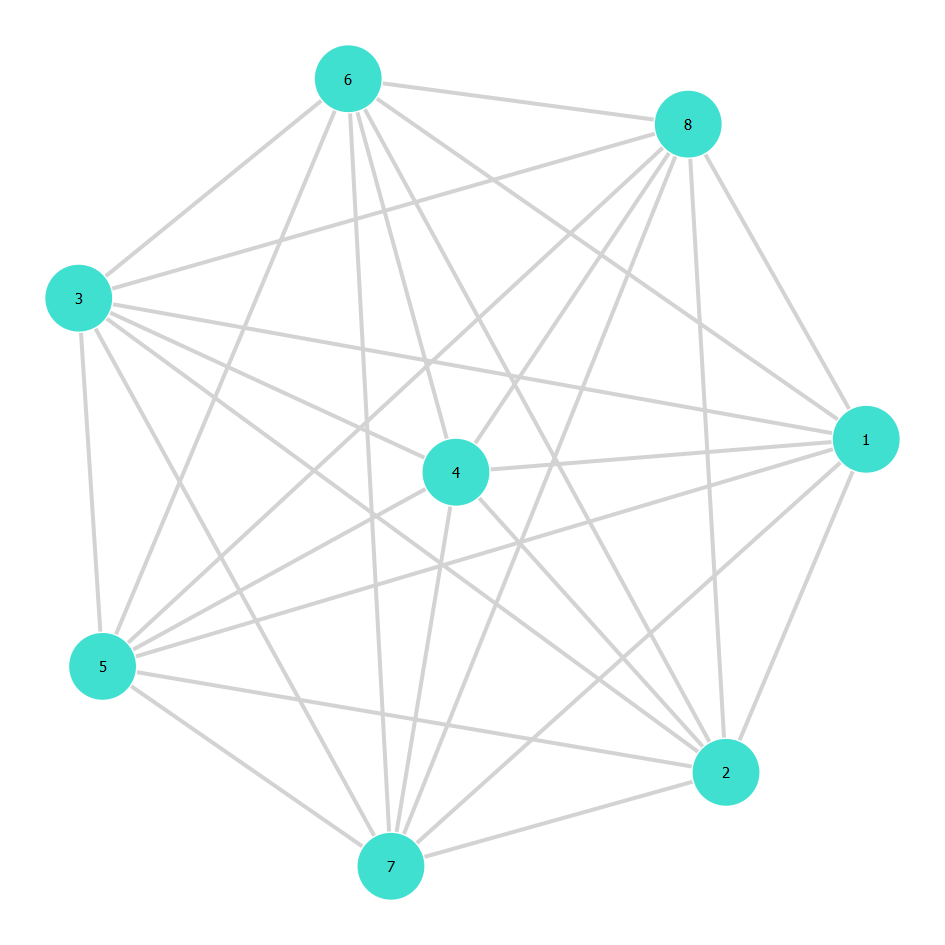
(b)

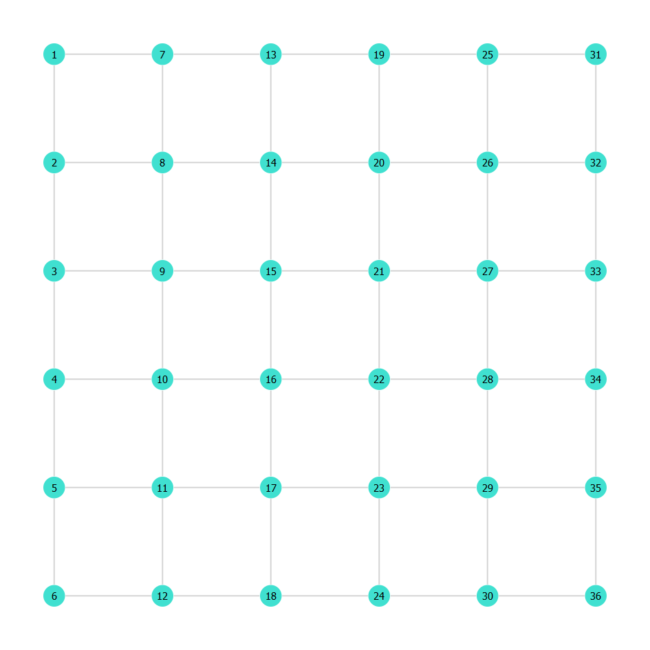
(c)

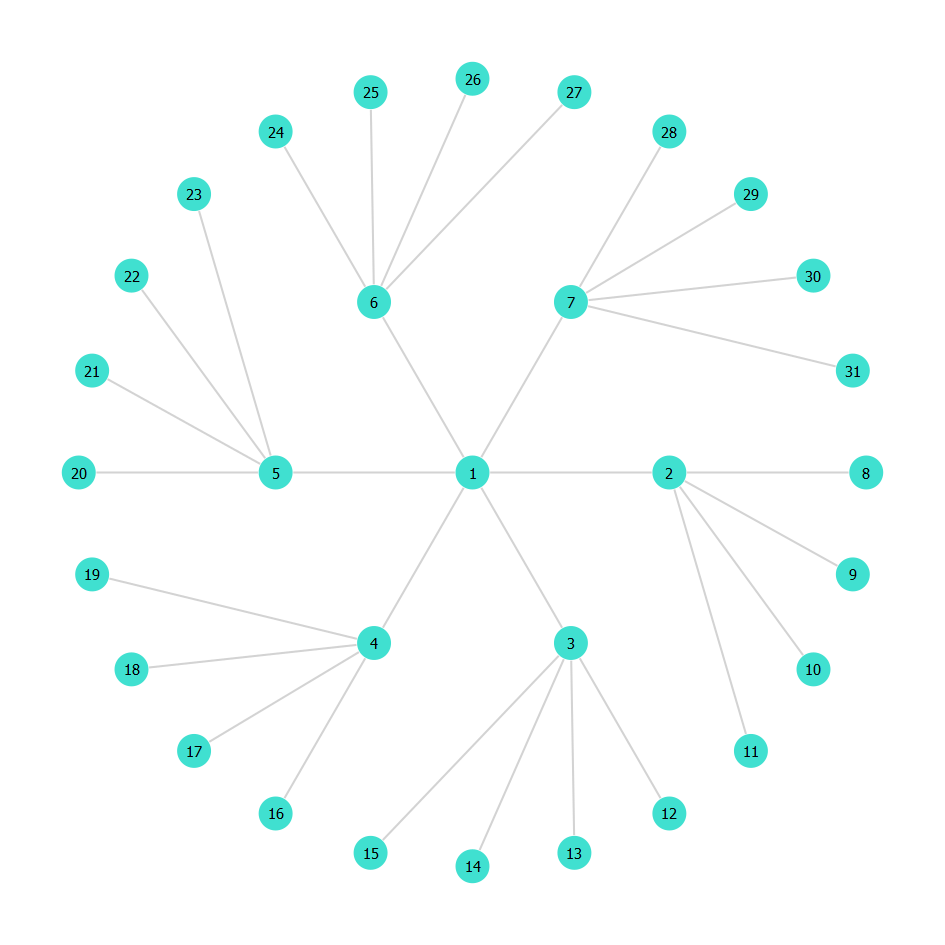
Figure 2: Examples of some network topologies, (a) A complete graph of 8 vertices, (b) A $6\crossproduct 6$ lattice graph, (c) A balanced tree graph with branching parameters of 6 and 4 at depth 1 and 2 respectively.

A complete graph shown in Fig. 2(a) offers maximum connectivity as every node is linked to each other [11]. This lessens the need for quantum memories and makes path-finding effortless. However, this topology is impractical for large-scale networks as the number of edges scales quadratically with the number of nodes, resulting in high infrastructure costs,

$$|E|=\frac{|V|^{2}-|V|}{2} \text{diameter}=d=1.$$ (11)

where $|E|$ is the number of edges and $|V|$ is the number of vertices in the graph. Another example illustrated in Fig. 2(b) is the lattice topology, a $m\crossproduct n$ dimension grid, whose edges increase linearly with the number of vertices in each dimension. The lattice topology is advantageous for accommodating multiple user pairs because it offers numerous routing options. However, it has a significant drawback in network optimization. As the network size increases, the shortest path becomes longer, which increases the path cost significantly. [11],

$$|E|=m(n-1)+n(m-1) d=\mathcal{O}(m+n).$$ (12)

A tree topology shown in Fig. 2(c) is an elementary topology characterised by depth and branching parameters. They are inherently acyclic and have only one path between two nodes. Its edges increase linearly with the number of vertices, but diameter scales logarithmically [11],

$$|E|=|V|-1 d=\mathcal{O}(\log(|V|)).$$ (13)

A major disadvantage of tree topology is its vulnerability to failure, which makes it unsuitable for multi-user quantum networks. On the other hand, thin trees have proven beneficial for studying path optimisation algorithms like asymmetric travelling salesman problems [28].

II.6 Shortest path routing

In his 1959 proposal, Dijkstra introduced an effective algorithm to determine the shortest path in any given graph [29]. The algorithm involves making multiple decisions to identify the path with the lowest cost. For example, in Fig. 3, if we begin at source point ‘A’, the algorithm will search for the path with the least cost and follow it to the next node, repeating the process until it reaches destination ‘B’. The algorithm has a maximum run-time of $\mathcal{O}(|V|^{2})$, which is applicable to Dijkstra’s implementation. It has been improved with a run time of $\mathcal{O}(|E|+|V|\log(|V|))$. Dijkstra’s shortest path algorithm takes a heuristic approach towards path finding between single-user pairs. Therefore when we scale this algorithm to multiple users, the problem becomes a vehicle routing problem which is a known NP-hard problem [11]. Hence, a complete multi-user optimisation is optional.

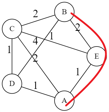
Figure 3: Shortest path routing manifesting in a network.

II.7 Multi-path routing

The traditional internet uses User Datagram Protocol (UDP) and the repeat-until-success method to ensure packet distribution [11]. Therefore, the classical internet relies on the shortest path between source and destination. Multiple paths in classical routing are of particular interest because they can make the network more resilient towards attacks by improving end-to-end data delivery [30]. In quantum internet, the guarantee of packet distribution is associated with the fidelity of the entangled pairs shared between end users.

Quantum network uses multiple paths to improve end-to-end delivery but also provides fault-tolerant infrastructure for multi-user quantum communication and distributed quantum computation. Entangled pairs between the source and destination from each path will incur some cost regarding channel loss or dephasing. These pairs, when purified, will generate a smaller quantity of entangled pairs but with very high fidelities [31]. Multi-path routing aims to use more than just the shortest path to maximise the network’s ability to support entanglement purification. This approach generates high-fidelity Bell pairs by purifying Bell pairs from different routes [32, 23, 22]. Therefore, quantum networks heavily rely on the multi-path routing of entangled pairs to obtain high fidelity, which makes longer paths less of a concern.

II.8 Quantum memories

Quantum memories are the key ingredient for quantum networks [5] and quantum repeaters [33, 34] to store and release the entangled pair at a desired time. In principle, an ideal quantum memory can absorb and re-emit the state of every single photon, which can be checked by counting the photons. In reality, memories can introduce decoherence because they tend to fail in re-emitting the state, or they can emit a state that is not a perfect match of the photon state stored in the memory. This will give rise to an efficiency-fidelity trade-off for using quantum memories to add value to our routing strategy [34]. Hence the cost of using memory is a cost vector of its own.

Quantum repeaters use memories to distribute entanglement over long distances, with considerably high bounds on efficiencies and fidelities. Still, bounds on efficiency are less demanded than on the fidelity of the path [35]. Thus, their use as a resource for realising large-scale communication adds a cost to the CVA when figuring out routing paths. The network graph bounds multi-path/multi-user algorithms. As a network can only accommodate a limited number of user pairs at a given time, it restricts the scalability of the graph.

II.9 Introduction to the QuNet package

QuNet is an open-source Julia language-based package for simulating and benchmarking quantum entanglement distribution networks via entanglement routing algorithms, available at GitHub. Other quantum network simulators considering different settings include NetSquid [36], QuNetSim [37], SimulQron [38]. All network simulators have some common features and some differences. QuNet differs from them because it takes an approach of quantum cost vector analysis. This helps simulate various quantum channels that can conform to the abelian nature and thus can be expressed as additive cost via weighted graphs, allowing us to exploit many graph routing algorithms [22].

In QuNet, the multi-path routing algorithm takes a greedy approach, using Dijkstra’s algorithm to find the shortest path that can be utilized in each iteration. The algorithm removes the path from the network to avoid repetition in subsequent iterations. In Fig. 4(a), there are two paths between nodes ‘A’ and ‘B’, with the red being the shortest and the blue being the next shortest. The multi-user algorithm is a more generalized form of the multi-path algorithm [22], aiming to maximize the graph’s utilization. The network graph $G$ is partitioned into $n$ sub-graphs, $G_{i}$ for $i\in\{1,\dots,n\}$. Each sub-graph contains a source node, a destination node, and all the paths used between them while adhering to specific rules,

$$G=\bigcup_{i=1}^{n}G_{i}\quad,\quad G_{i}\cap G_{j}=\emptyset\quad,\quad\forall\{i\neq j\}.$$ (14)

(a)

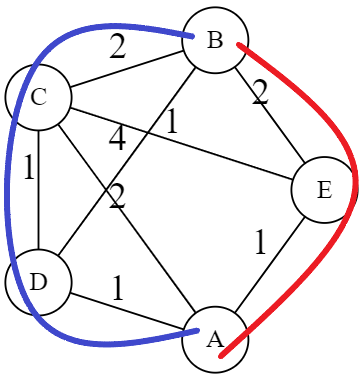
(b)

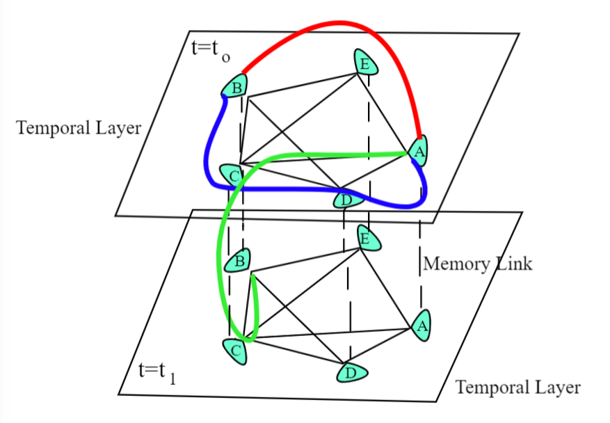
Figure 4: (a) Multi-path routing strategy, (b)Temporal multi-path routing strategy manifesting in a network.

This approach does not require tracking of qubits and therefore bypasses some quantum complexities, but it only needs bookkeeping of cost vector. QuNet finds the optimal route between end users based on cost vector analysis, so an entanglement link can be created between them by performing entanglement swapping and purification.

QuNet simulates quantum memories as temporal links as swapping and purification protocol between user pairs are not time-sensitive [22]. Thus, temporal routing guarantees a path between each user pair by routing entanglement at different times when the path is available. An asynchronous routing scheme [22] is given in Fig. 4(b). Here, ‘A’ and ‘B’ establish entanglement using three paths. The entangled pairs are transmitted at some instance $t_{0}$ through red and blue paths, but no more paths are available. Temporal routing allows the entangled pairs to traverse to another temporal layer at time $t_{1}$. Here the link between ‘C’ and ‘B’, which is clogged up in the blue path, is freed to be used in the green path. Thus, guaranteeing a path at the expense of higher costs.

Some features of QuNet are scalability, user interface, dynamic simulators and abstraction [22].

• Scalability: QuNet heavily uses Dijkstra’s algorithm to find paths in any network. This makes it computationally efficient, which is beneficial for large-scale networks.

• User Interface: QuNet performs routing algorithms on a quantum network that constitutes quantum nodes and channels, irrespective of the graph type.

• Dynamic Simulators: QuNet provides a variety of quantum channels like fibre optic channels, free space channels, and satellite channels. It also accounts for a quantum node that is not stationary by updating the cost vector at regular intervals.

• Abstraction: quantum network entities QNode and QChannel are kept independent of the technological constraints so that they can take arbitrary forms. For instance, it does not account for node losses from performing procedures like swapping and purification. Although, QuNet allows the user to extend the existing paradigm and include them in cost vectors to simulate a real-world network.

III Scaling for different network topologies for multi-path in multi-user networks

The present section presents our research findings on quantum network analysis, an area of paramount importance in quantum information. Available quantum relay networks are primarily based on two topologies, namely Point-to-Point (P2P) and Star. The problem with such topologies is that they do not support multi-path routing entanglement. The closest contender widely studied is lattice topology. It is not an effective choice because when multiple user pairs join the quantum network, the pathfinding becomes competitive, and paths in lattice scale bi-linearly in $X$ and $Y$ dimensions. We propose a topology that is not only suitable for large-scale quantum repeater networks but is relatively effective when scaled to high-user competition scenarios. We call it a "connected tree", which incorporates redundant rings of edges at each level of the existing tree network to support multiple user pairs. The connected tree has twice as many edges as the associated tree graph, with $|E|=2(|V|-1)$. By overcoming the tree network’s acyclic nature limitation, the connected tree provides greater flexibility for accommodating user pairs and enables more paths between users. Specifically, our study highlights the fundamental role that network topologies play when scaling quantum networks for protocols, such as multi-user quantum key distribution and distributed quantum computing.

Our research showcases the proof of concept for scalability and multi-path routing in tree topologies, as discussed in Sec. III.1. Furthermore, we demonstrate in Sec. III.2 the significant impact that edge schemes of topology have on network statistics. In Sec. III.3, we compare the effect of network topologies on quantum network statistics. In Sec. III.4, we exhibit the influence of the multi-user routing scheme on quantum key distribution networks with various topologies. Lastly, in Sec. III.5, we apply our research findings to a network of universities in Islamabad, Pakistan, and compare different topologies.

III.1 Proof of principle of adding redundant edges in tree networks

Proof of principle emphasises the importance of redundant edges in tree topology and the need for quantum memories to accommodate multiple user pairs in the network. The acyclic nature of the tree graph makes it a good candidate for single-path routing between a user pair, but all the nodes in that single will now only act as repeater nodes. This leads to the catastrophic failure of tree topology in multi-user competition. Adding redundant edges to the topology in a specific manner, i.e. a ring of edges connects each node at a given depth, will allow a user pair to opt for multi-path routing of entangled pairs. These redundant edges remove the tree topology’s acyclic nature and help accommodate more user pairs to support multi-user routing. Previously, it has been shown for lattice networks [22], and here it is extended to tree networks.

Tree networks only have one path between any two nodes, causing simple routing algorithms like Breadth First Search (BFS) and Depth First Search (DFS) to find the shortest path efficiently.

(a)

(b)

Figure 5: A graphical representation of tree topologies. (a) a balanced tree with three depth levels with a branching ratio decreasing at each depth, (b) a connected tree made by adding concentric rings of edges at each depth.

Pathfinding in tree graphs is relatively easy for a single-user pair. However, as we scale the graph, the shortest path-finding problem becomes a vehicle rescheduling problem [11]. A connected tree topology is used to overcome it, which can accommodate more user pairs by providing more routing options.

(a)	(b)
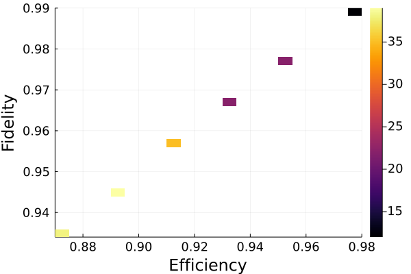
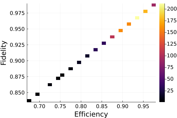
(c)	(d)

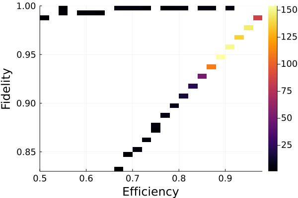
Figure 6: Trade-off is shown between fidelity of entangled pairs and the efficiency of the path/paths used to share pairs between source and destination. (a), (c) and (b), (d) shows the single path and Multi-path routing respectively

41 node tree topologies are shown in Figs. 5(a) and (b). Both networks are simulated with similar edge costs of $0.1$ dB depicting loss and dephasing channels. QuNet is used to find paths between $20$ user pairs for $100$ trails. The only variable parameter for proof of principle is the number of allowed paths between each user pair.

Fig.6 illustrates routing data for the shortest path and two paths of entangled pairs. The QuNet ran the simulation 2000 times, but as shown in Figs. 6(a) and (b), the feasible paths in tree topology are scarce. The linear distribution of path cost data confirms that the tree fails to provide multiple paths and accommodate multiple users. Whereas from Figs. 6(c) and (d), it can be extrapolated that connected tree provides a considerably large number of routing options than trees. The connected tree topology can also accommodate more user pairs because of the removal of acyclic bound. In Fig. 6(d), apart from the linear distribution of path data, these outliers represent the use of two paths. The advantage of multi-path routing arises from entanglement purification, where a gain in fidelity is achieved at the expense of decreased efficiency.

III.2 Impact of Edge Scheme on Scalability

For any global quantum server, scalability is a great challenge. QuNet being a contender for simulating larger-scale entanglement distribution networks, takes the support of redundant edges. Here an idea is presented that the edge scheme of topology plays a significant role in network statistics, i.e. performance or path finding in user competition.

We use a connected tree topology of 65 nodes to show scalability, with $2(65-1)=128$ edges. Fig. 7(a) is a connected tree with just one depth that has 64 nodes connected to one central node Fig. 7(d) has two depths, the first one with $8$ nodes while the second one has a branch parameter of $7$, and Fig. 7(g) has three depths with branching ratios of $4,3$ and $4$. To present the effects of topologies, all test networks are simulated with each edge having two weights/costs, ‘loss’ and ‘Z (dephasing)’, with an arbitrary value of $0.1\text{dB}$. Each network is tested with three temporal layers, where costs of loss and dephasing from utilising quantum memory vary arbitrarily from $0.1\text{dB}$ to $0.9\text{dB}$. Each user pair can use three paths to route their entangled pairs.

(a)

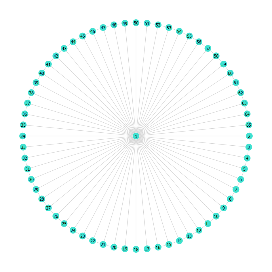
(b)

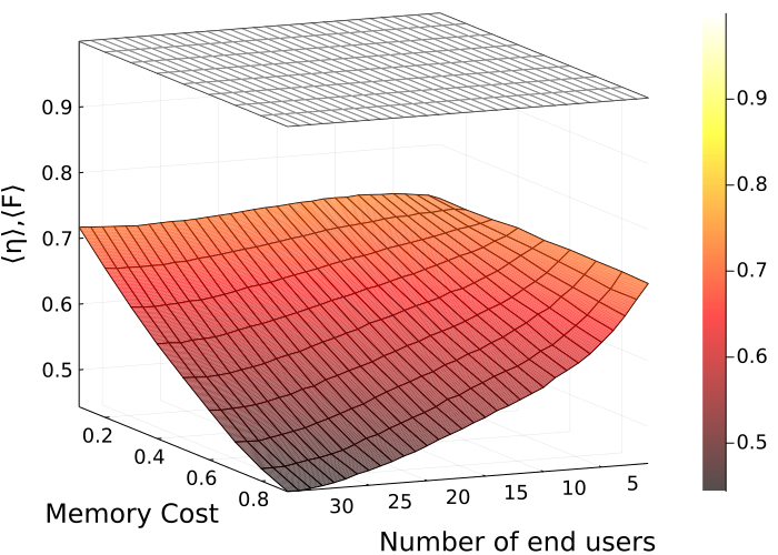
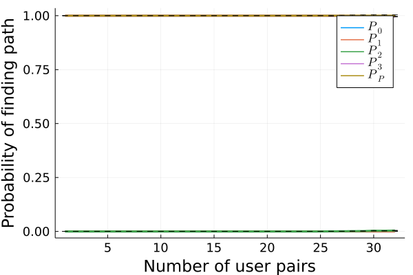
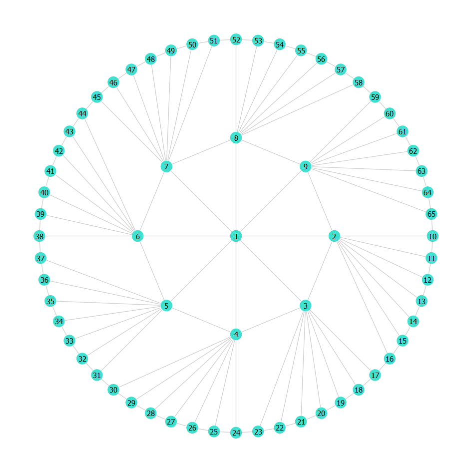
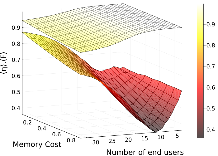
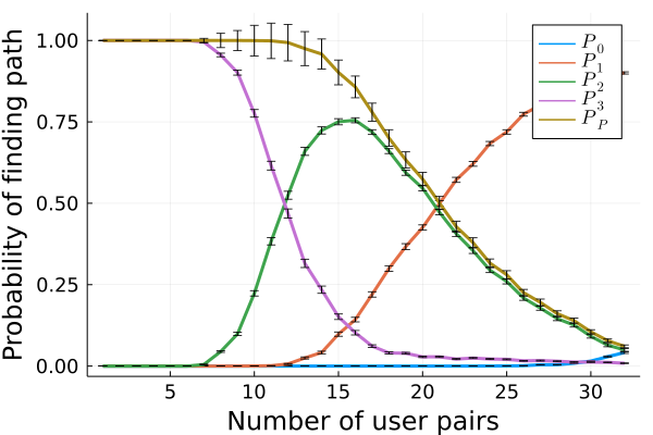
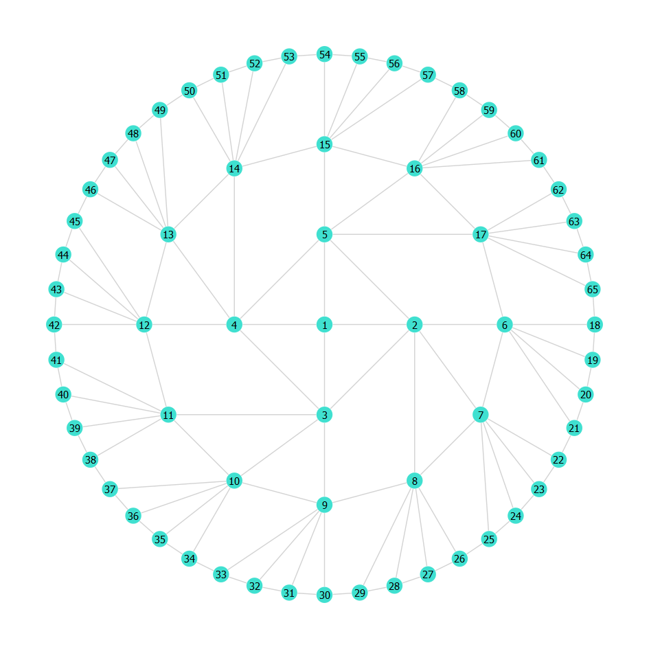
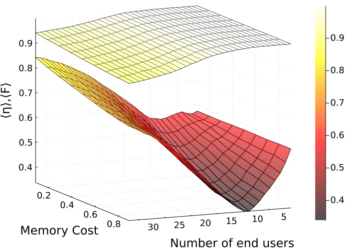
(c) (d) (e) (f) (g) (h) (i)

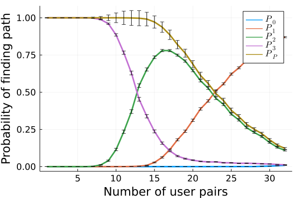
Figure 7: Three different edge schemes in connected tree topology are presented to make three different topologies. Each Topology has $65$ nodes, $128$ edges each with the weight of $0.1dB$ for both loss and dephasing, and the network statistics were collected for $500$ trials. Each user pair was allowed to use $3$ paths to send their entangled pairs, and they could utilise $3$ different temporal layers. (c), (f) and (i) are plotted for path probabilities and path purification behaviour. In network performance plots (b), (e), and (h), the lower surface represents efficiency, and the upper surface represents fidelity.

The probability of purifying entangled pairs from multiple paths

$$P_{P}=\frac{\sum_{n\geq 2}P_{n}}{(1-P_{0})}.$$ (15)

depends on the probability of using $n$ number of paths $P_{n}$ and the probability of finding zero paths $P_{0}$.

It can be observed from Figs. 7 (b), (e), and (f), that the average efficiency between the number of user pairs decreases till the purification threshold. This reflects the ability of a graph to accommodate multiple user pairs, with most of them opting for multi-path routing. However, the average efficiency of the network decreases due to longer paths traversed. Pairs must use single-path routing at the user threshold to accommodate maximum user pairs. The increase in efficiency after the purification threshold indicates that user pairs are resorting to shortest-path routing. Any more user pairs will have higher chances of not finding any path to route their entangled pairs.

Depth	Branches	Purification Threshold	User Threshold
1	64	none	none
2	8,7	10	27
3	4,3,4	13	29
4	3,2,3,2	15	32

Table 1: This table shows how the different edge schemes affect network thresholds.

According to the Table. 1, it is clear that networks with more depths give better outcomes in a connected tree topology. The edge scheme of a graph is essential not only for network performance but also for finding paths between user pairs. Fig. 7(c) shows that the edge scheme of Fig. 7(a) is highly beneficial for accommodating all the user pairs. This edge scheme links any two nodes by traversing through only two edges. The additional advantage of temporal routing in three layers makes it suitable for user accommodation. Pathfinding in Fig. 7(d) and (g) is different from Fig. 7(a) because they have extra depths. Here the user pairs compete to find paths as shown in Fig. 7(f) and (i). However, the network with three depths has more significant thresholds for purification and user accommodation at the expense of low efficiencies.

III.3 Impact of Network Topology on Q-Network Statistics

In the previous section, we discussed the effects of different edge schemes on network statistics. Here a comparison is presented between two fundamental topologies that are inherently different regarding several edges and edge schemes, including temporal routing, to simulate the effect of quantum memories. To make a fair comparison, a network of 64 users is assumed in two different topologies: a connected tree with $4$ branches and $126$ edges in Fig. 8(a), and an $8\crossproduct 8$ lattice(grid) with $112$ edges in Fig. 8(b). All other variables like edge costs, number of trials, temporal layers, memory costs, and number of allowed paths per user pair are kept constant, as defined in Sec. III.2.

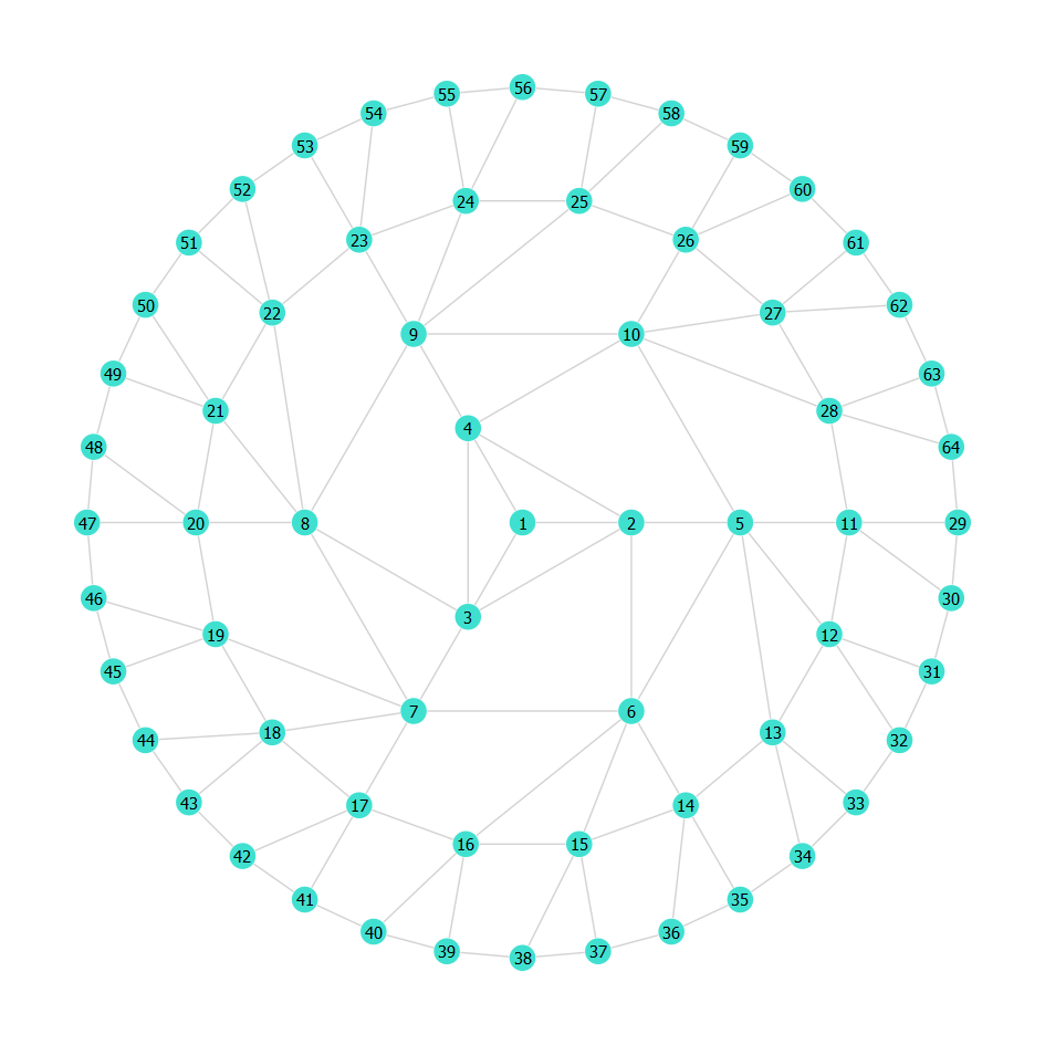
(a)	(b)
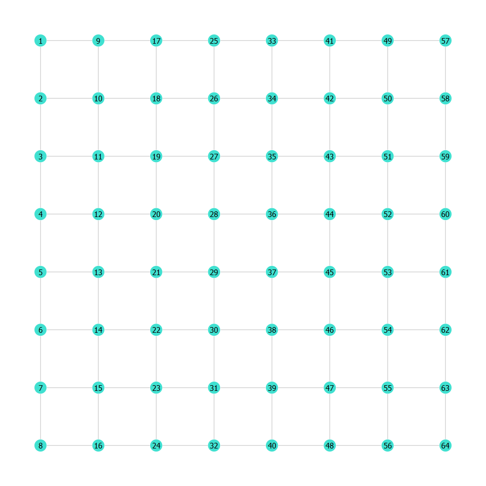
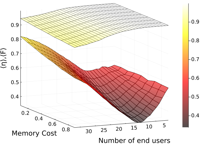
(c)	(d)
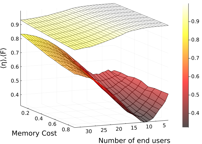
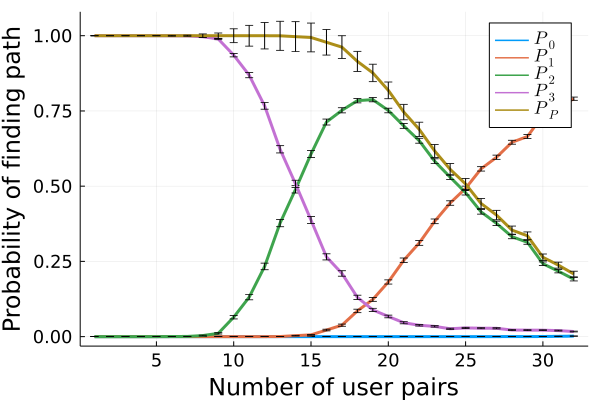
(e)	(f)
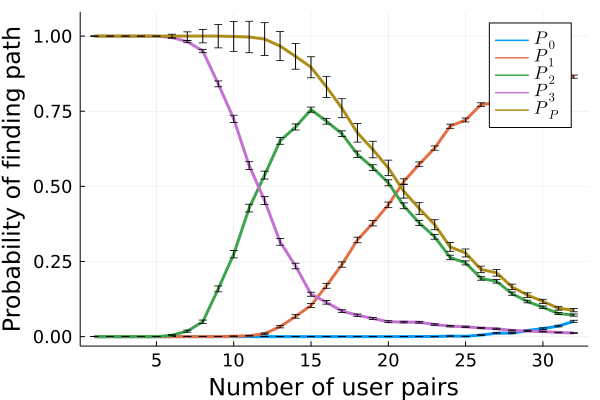
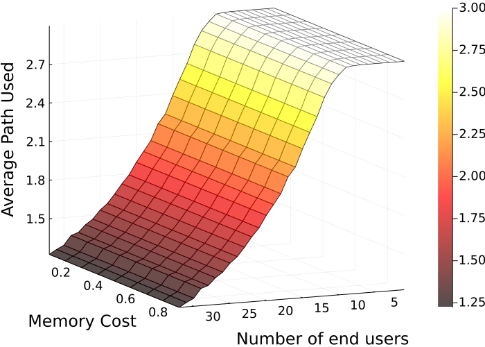
(g)	(h)

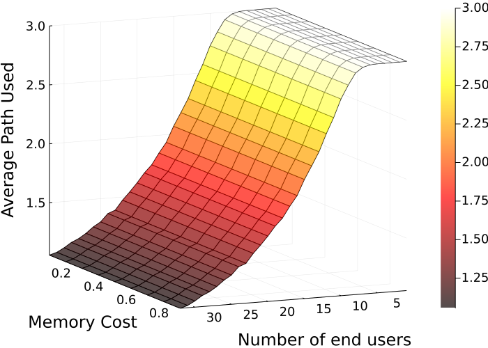
Figure 8: Path routing and network statistics for 64 node topologies. One is a connected tree with 126 edges in four depths with branching parameters of 3,2,3, and 2, respectively, and the other is a lattice network with 112 edges. (a),(b) shows the edge scheme in the network, (c) (d) shows the average performance of the network versus user competition and memory cost, where the lower surface presents efficiency, and the upper surface represents average fidelity between user pairs. (e),(f) shows an account of probabilities for path opting strategy versus user competition, and (g) (h) shows average paths used by each user pair versus user competition.

As observed from Figs. 8(c) and (d), the average network performance of a connected tree is by far better than that of a lattice. The efficiency surface graph of the connected tree is less steep than the lattice’s, which indicates that the network is more resilient toward user competition and provides more options to route entangled pairs to each user pair. Multi-path routing, which provides a good gain in fidelity between end users, also worsens the net efficiency between each user pair [22].

Even though the less steep efficiency surface of the connected tree indicates higher chances of multi-path routing, it still gives better results than lattice at the low competition. This behaviour is plausibly explainable by path optimisation algorithms; for any user pair, the number of channels traversed is lesser than travelled in the lattice. Therefore, finding the shortest path in the connected tree is shorter than in the lattice. When using multi-path routing for multiple user pairs, the network needs to be resilient and scalable, represented by the purification and user threshold. Connected tree and lattice topologies are both good candidates for multi-user entanglement distribution. However, from Figs. 8(e) and (f), we see that the purification threshold reaches quickly for lattice at merely 10 user pairs, whereas the connected tree accommodates 14 user pairs before the threshold. Furthermore, The user threshold is also better for connected tree topology than lattice, i.e. 31 and 25, respectively. This depicts that the connected tree is more tolerant and accommodates more user pairs with a higher chance of providing multiple paths than lattice.

The average path supports these observations based on probabilities visualised in Figs. 8(g) and (h). On average, three paths are used by seven user pairs in the lattice and nine in the connected tree, two paths by 16 user pairs in the lattice and 19 in the connected tree. Both networks provide at least one path to all 32 user pairs, provided that networks have three temporal layers.

III.4 Impact of Network Topology on Secret Key Rates in QKD

As shown earlier, networks behave differently when scaled to higher user competition environments. The aim is to see how the QKD secret key rates are affected by network topology, comparing results for a lower number of user pairs preferring multi-path routing to a higher number of user pairs that are more prone towards single-path routing. Now for applicability, networks shown in Sec. III.3 are made test beds for quantum communication via distributing a secret key between each user pair through quantum key distribution protocol. An ideal approach is used where the users perform operations that do not add decoherence. Thus, all the errors can be accounted for by the paths used.

To calculate the secret key rate, we use the raw qubit rate [22],

$$R=\frac{M(1-P_{0})\langle\eta\rangle}{\tau},$$ (16)

where $M$ is the number of user pairs in the network, and $P_{0}$ is the probability of the network failing to provide a single path between a user pair. $\langle\eta\rangle$ is the average efficiency of the path/s each user pair chooses to send their entangled pairs. Lastly, $\tau$ is the number of temporal layers available to user pairs to ensure maximum success in finding a route. As for the QKD secret key rate per user pair, we use [39]

$$C =R(1-\mathcal{H}(\varepsilon))$$

$$=\frac{(1-P_{0})\langle\eta\rangle}{\tau}\Big{[}1-\mathcal{H}(1-F^{{}^{\prime}})\Big{]}.$$ (17)

Here $\mathcal{H}(1-F^{{}^{\prime}})=F\log_{2}(F^{{}^{\prime}})-(1-F^{{}^{\prime}})\log_{2}(1-F^{{}^{\prime}})$ is the entropy and $F^{{}^{\prime}}$ is the fidelity after purification. With this, networks are simulated to observe user competition and network topology effects on QKD rates.

(a)
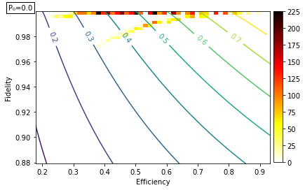
(b)
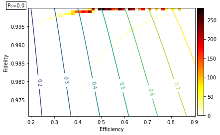
(c)
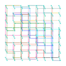
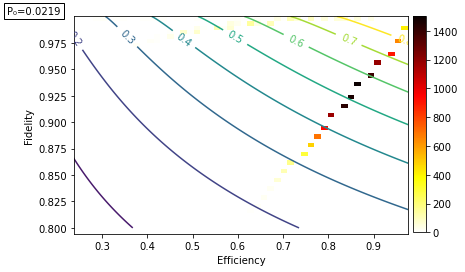
(d)

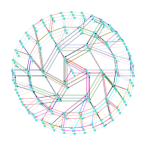
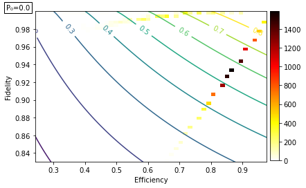
Figure 9: Network topologies with three temporal layers are shown adjacent to their graphical representation of routing data opted by user pairs in 500 trials, with an overlay of contours depicting QKD secret key rates. The networks are simulated for low user competition of 10 user pairs for (a) $8\crossproduct 8$ lattice and (b) $4$ depth connected tree and for high user competition of 30 pairs for (c) $8\crossproduct 8$ lattice and (d) $4$ depth connected tree

The user competition and topology of the simulated network affect the path selection between user pairs, affecting the secret key generation rates.

It can be observed from the routing data shown in Fig. 9(a) that out of 10 user pairs, some choose to use two rather than three paths. Efficiencies of paths in the lattice are spread over a wide range, with few being more significant than others. This means user pairs far apart in lattice have greater costs for multi-path routing. Therefore, such pairs can distribute a secret key through QKD but will have to succumb to lower key rates. Conversely, some user pairs are close and can share a key with a very high key generation rate. Most of the routing data give key rates below $0.5$ due to the very high-efficiency cost, indicating that the poor choice of paths provided by the network decreased the output key rate. On the other hand, the connected tree in a low competition environment, shown by Fig. 9(b), benefits from the topology to provide a shorter path between user pairs. Hence most of the routing data have better efficiency costs. The key rates generated by them are better than $0.5$ even with multi-path routing.

In high-user competition, both networks behave somewhat similarly. Still, the lattice has a slight chance of almost $2\%$, where it can fail to provide a path between user pairs, thus affecting the overall purpose of networking. From Fig. 9(c), it is observed that when lattice becomes saturated with user pairs, it prefers single path routing with optimised routes, thus providing better efficiency costs resulting in improved key rates. For example, the connected tree topology shown by Fig. 9(d), where it was easier to optimise routing paths, maintains the trend of better paths for QKD rates in single path routing as well, with a few user pairs having the luxury of multi-path routing.

III.5 Simulating Entanglement Distribution Networks in Islamabad for QKD with Different Topologies

Given the premise that multi-path routing and network topology plays a crucial role in future multi-user entanglement distribution networks to accommodate the desired number of user pairs with feasible efficiency-fidelity trade-off. Here, insight is given by making two significantly different networks for $14$ universities in Islamabad, the capital city of Pakistan.

Now in real-world networks, each edge will not be the same. Some will be longer than others, affecting the costs of utilising those edges. So for the Islamabad network, we made the edge costs dependent on the shortest distance between the two nodes that the edge joins, along with a base cost of $0.1\text{dB}/\text{km}$. One of the two networks simulated for Islamabad is a minimal spanning tree (MST) with $13$ edges. This is one of the most common topologies used for multi-node P2P networks. By definition, it is a graph that joins all the nodes with a minimum number of edges. The other is a network with $91$ edges based on a complete graph that connects each node with every other node, thus providing at least one path to each user pair at any given moment.

	(a)
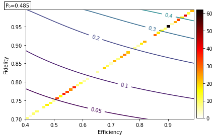
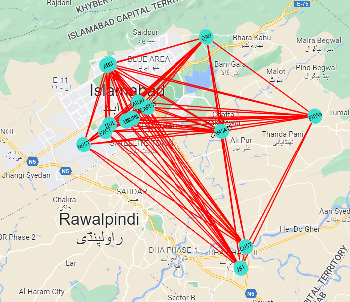
	(b)

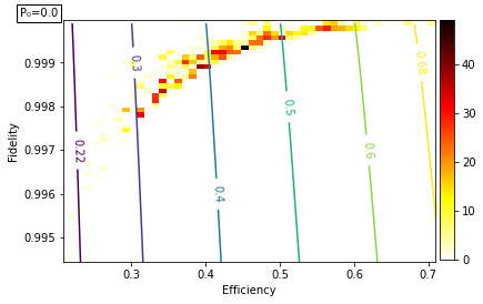
Figure 10: (a) A minimal spanning tree network that has a $61.37km$ total optic fibre channels, (b) A connected graph network that has a $1109.67km$ total optic fibre channels. Efficiency-Fidelity routing path data overlayed with QKD secret key rate contours showing a linear distribution for the trade-off. The network was simulated for $500$ trials and $3$ user pairs. It was found to fail almost $49\%$ of the time to provide a single path to the user pair.

An MST-like topology will likely fail around 49% times in providing a path to anything greater than one user pair. Therefore, when simulated for $500$ trials, the routing path data between 3 user pairs is linearly distributed. Grouping in data might be due to the higher cost for longer paths between far-away user pairs. That utilises many channels at lower efficiency-fidelity regions, and shorter paths between closer or neighbouring user pairs have auspicious values for fidelity and efficiency. The high chance of failure makes MST a terrible candidate for a multi-user entanglement distribution network. This means that even though user pairs might be neighbouring, there is a strong chance that those channels are already under use by some other user pair, rendering it useless. Thus, meagre secret key rate generation rates were expected from Fig. 10(a).

The complete graph (CG) projects a different trade-off than MST. The CG network has around $91$ channels with a very high net length which guarantees multi-path routing leading to low collective path efficiencies but high fidelities. The key generation rate per user pair improves because all three user pairs have many options for path routing. This improvement causes the complete graph to surpass MST in QKD key rate at very low efficiencies, as seen in Fig. 10(b).

IV Discussion and Conclusion

We have proposed an alternate for quantum network topologies, the connected tree, which proves to be far more effective than its counterpart lattice. The advantage of building a quantum internet is purifying entangled pairs from multiple paths into high-fidelity entangled pairs between each user pair. Networks like stars and P-2-P would not be beneficial for useful entanglement distribution. Lattice is the next proposed choice, but our analysis shows that it falls behind in providing fruitful entanglement to everyone in the network. It is evident from the study that a connected tree is a more fault-tolerant topology and favourable for scalable entanglement distribution. From a perspective of resources, it also outperforms lattice by providing shorter paths, accommodating more user pairs, and providing more routing options with the least usage of quantum memories.

In conclusion, the findings presented in this study highlight the significance of topology, edge scheme, and multi-path routing in the design and optimization of entanglement distribution networks for scalable quantum internet applications. The research focused on comparing the performance of connected tree and lattice networks with different edge schemes in terms of multi-user routing, path optimization algorithms, and quantum key distribution (QKD) rates. The simulations demonstrated that a connected tree topology with redundant edges outperforms the acyclic tree structure by providing multiple paths between a larger number of user pairs. By maximizing the depth of the primary tree network, the connected tree topology offers increased routing options at the cost of some channel losses. This was supported by the analysis of network statistics, which revealed an increasing trend of purification and user thresholds with increased depth in the connected tree network.

Furthermore, the study emphasized the importance of network topology in path optimization algorithms. While both lattice and connected tree networks accommodated the same number of user pairs, the lattice network exhibited poor average path efficiencies due to a higher number of channels being traversed, especially under low user competition. In contrast, the connected tree topology showed superior performance in terms of average path efficiencies and the ability to establish multiple routes between user pairs. The research also demonstrated the significant impact of multi-path routing on QKD rates. Multi-path routing facilitated the establishment of entanglement through multiple paths, which could later be purified to serve as a single shared entanglement. This resulted in higher secret key rates per user-pair, proving beneficial in low- and high-user competition scenarios. Comparatively, the connected tree topology yielded better QKD rates with its ability to provide more routing options while traversing fewer channels than the lattice.

These findings hold practical implications for engineers and scientists involved in quantum networking, as they provide valuable insights for resource allocation and optimisation. The study exemplified this by presenting a network design for Islamabad, Pakistan, which showcased the cost-effectiveness of different topologies. Although cheaper, the minimal spanning tree (MST) topology could only provide a single path to one user pair, leading to a high probability of failure in multi-user routing and a poor efficiency-fidelity trade-off. In contrast, despite its higher monetary cost, the complete graph guaranteed multi-path routing even at saturation points, resulting in significantly better QKD secret key rates. In summary, this study underscores the importance of considering topology, edge scheme, and multi-path routing in the design of entanglement distribution networks, which serve as the foundation for scalable future quantum internet architectures. By leveraging these insights, engineers and scientists can make informed decisions and maximise quantum communication systems’ efficiency, reliability, and scalability.

V Acknowledgements

The authors thank and acknowledge Dr Peter P. Rohde for many fruitful discussions. His insights were extremely helpful in structuring this study.

Data Availability Statement

The data supporting this study’s findings are available from the corresponding author upon reasonable request.

Conflict of Interest Statement

The authors have no conflict to disclose.

References

- Bennett and Brassard [2014] C. H. Bennett and G. Brassard, Quantum cryptography: Public key distribution and coin tossing, Theoretical Computer Science 560, 7 (2014), theoretical Aspects of Quantum Cryptography – celebrating 30 years of BB84.
- Nielsen and Chuang [2010] M. A. Nielsen and I. L. Chuang, Quantum Computation and Quantum Information: 10th Anniversary Edition (Cambridge University Press, 2010).
- Lauk et al. [2020] N. Lauk et al., Perspectives on quantum transduction, Quantum Science and Technology 5, 020501 (2020).
- Munro et al. [2019] W. J. Munro, N. L. Plparo, and K. Nemoto, Quantum multiplexing, in 2019 Conference on Lasers and Electro-Optics (CLEO) (2019) pp. 1–2.
- Kimble [2008] H. J. Kimble, The quantum internet, Nature 453, 1023 (2008).
- Chen et al. [2021] Y.-A. Chen et al., An integrated space-to-ground quantum communication network over 4,600 kilometres, Nature 589, 214 (2021).
- Stucki [2011] D. Stucki, et al., Long-term performance of the swissquantum quantum key distribution network in a field environment, New Journal of Physics 13, 123001 (2011).
- Peev [2009] M. Peev, et al., The secoqc quantum key distribution network in vienna, New Journal of Physics 11, 075001 (2009).
- Ruihong and Ying [2019] Q. Ruihong and M. Ying, Research progress of quantum repeaters, Journal of Physics: Conference Series 1237, 052032 (2019).
- Valivarthi [2020] R. Valivarthi, et al., Teleportation systems toward a quantum internet, PRX Quantum 1, 020317 (2020).
- Rohde [2021] P. P. Rohde, The Quantum Internet: The Second Quantum Revolution (Cambridge University Press, 2021).
- Chou et al. [2007] C.-W. Chou, J. Laurat, H. Deng, K. S. Choi, H. de Riedmatten, D. Felinto, and H. J. Kimble, Functional quantum nodes for entanglement distribution over scalable quantum networks, Science 316, 1316 (2007), https://www.science.org/doi/pdf/10.1126/science.1140300 .
- Yuan et al. [2008] Z.-S. Yuan, Y.-A. Chen, B. Zhao, S. Chen, J. Schmiedmayer, and J.-W. Pan, Experimental demonstration of a bdcz quantum repeater node, Nature 454, 1098 (2008).
- Kheirkhah et al. [2019] M. Kheirkhah, I. Wakeman, and G. Parisis, Multipath transport and packet spraying for efficient data delivery in data centres, Computer Networks 162, 106852 (2019).
- Munro et al. [2015] W. J. Munro, K. Azuma, K. Tamaki, and K. Nemoto, Inside quantum repeaters, IEEE Journal of Selected Topics in Quantum Electronics 21, 78 (2015).
- Sun [2016] Q.-C. Sun, et al., Quantum teleportation with independent sources and prior entanglement distribution over a network, Nature Photonics 10, 671 (2016).
- Autebert [2016] C. Autebert, et al., Multi-user quantum key distribution with entangled photons from an algaas chip, Quantum Science and Technology 1, 01LT02 (2016).
- Herbauts et al. [2013] I. Herbauts, B. Blauensteiner, A. Poppe, T. Jennewein, and H. Hübel, Demonstration of active routing of entanglement in a multi-user network, Opt. Express 21, 29013 (2013).
- Wang [2022] R. Wang, et al., A dynamic multi-protocol entanglement distribution quantum network, in 2022 Optical Fiber Communications Conference and Exhibition (OFC) (2022) pp. 1–3.
- Inagaki et al. [2013] T. Inagaki, N. Matsuda, O. Tadanaga, M. Asobe, and H. Takesue, Entanglement distribution over 300 km of fiber, Opt. Express 21, 23241 (2013).
- Yin [2017] J. Yin, et al., Satellite-based entanglement distribution over 1200 kilometers, Science 356, 1140 (2017), https://www.science.org/doi/pdf/10.1126/science.aan3211 .
- Leone et al. [2021] H. Leone, N. R. Miller, D. Singh, N. K. Langford, and P. P. Rohde, Qunet: Cost vector analysis and multi-path entanglement routing in quantum networks (2021), arXiv:2105.00418 [quant-ph] .
- Proctor et al. [2018a] T. J. Proctor, P. A. Knott, and J. A. Dunningham, Multiparameter estimation in networked quantum sensors, Phys. Rev. Lett. 120, 080501 (2018a).
- Proctor et al. [2018b] T. J. Proctor, P. A. Knott, and J. A. Dunningham, Multiparameter estimation in networked quantum sensors, Physical Review Letters 120, 10.1103/physrevlett.120.080501 (2018b).
- Bennett et al. [1996] C. H. Bennett, G. Brassard, S. Popescu, B. Schumacher, J. A. Smolin, and W. K. Wootters, Purification of noisy entanglement and faithful teleportation via noisy channels, Phys. Rev. Lett. 76, 722 (1996).
- Pan and Zeilinger [1998] J.-w. Pan and A. Zeilinger, Greenberger-horne-zeilinger-state analyzer, Phys. Rev. A 57, 2208 (1998).
- Pan et al. [1998] J.-W. Pan, D. Bouwmeester, H. Weinfurter, and A. Zeilinger, Experimental entanglement swapping: Entangling photons that never interacted, Phys. Rev. Lett. 80, 3891 (1998).
- Haji and Ramin [2018] M. Haji and S. Ramin, Thin trees in some families of graphs, Ph.D. thesis (2018).
- Dijkstra [1959] E. W. Dijkstra, A note on two problems in connexion with graphs, Numerische Mathematik 1, 269 (1959).
- Mustafa et al. [2012] H. Mustafa, X. Zhang, Z. Liu, W. Xu, and A. Perrig, Jamming-resilient multipath routing, IEEE Transactions on Dependable and Secure Computing 9, 852 (2012).
- Deutsch et al. [1996a] D. Deutsch, A. Ekert, R. Jozsa, C. Macchiavello, S. Popescu, and A. Sanpera, Quantum privacy amplification and the security of quantum cryptography over noisy channels, Physical Review Letters 77 (1996a).
- Sidhu and Kok [2020] J. S. Sidhu and P. Kok, Geometric perspective on quantum parameter estimation, AVS Quantum Science 2, 014701 (2020), https://doi.org/10.1116/1.5119961 .
- Briegel et al. [1998] H.-J. Briegel, W. Dür, J. I. Cirac, and P. Zoller, Quantum repeaters: The role of imperfect local operations in quantum communication, Phys. Rev. Lett. 81, 5932 (1998).
- Sangouard et al. [2011] N. Sangouard, C. Simon, H. de Riedmatten, and N. Gisin, Quantum repeaters based on atomic ensembles and linear optics, Rev. Mod. Phys. 83, 33 (2011).
- Simon et al. [2010] C. Simon et al., Quantum memories, The European Physical Journal D 58, 1 (2010).
- Coopmans et al. [2021] T. Coopmans et al., NetSquid, a NETwork simulator for QUantum information using discrete events, Communications Physics 4, 10.1038/s42005-021-00647-8 (2021).
- Diadamo et al. [2021] S. Diadamo, J. Notzel, B. Zanger, and M. M. Bese, QuNetSim: A software framework for quantum networks, IEEE Transactions on Quantum Engineering 2, 1 (2021).
- Dahlberg and Wehner [2018] A. Dahlberg and S. Wehner, SimulaQron—a simulator for developing quantum internet software, Quantum Science and Technology 4, 015001 (2018).
- Nemoto et al. [2016] K. Nemoto, M. Trupke, S. J. Devitt, B. Scharfenberger, K. Buczak, J. Schmiedmayer, and W. J. Munro, Photonic quantum networks formed from nv- centers, Scientific Reports 6, 26284 (2016).
- Bradley et al. [2019] C. E. Bradley, J. Randall, M. H. Abobeih, R. C. Berrevoets, M. J. Degen, M. A. Bakker, M. Markham, D. J. Twitchen, and T. H. Taminiau, A ten-qubit solid-state spin register with quantum memory up to one minute, Phys. Rev. X 9, 031045 (2019).
- Einstein et al. [1935] A. Einstein, B. Podolsky, and N. Rosen, Can quantum-mechanical description of physical reality be considered complete?, Phys. Rev. 47, 777 (1935).
- Bell [1964] J. S. Bell, On the einstein podolsky rosen paradox, Physics Physique Fizika 1, 195 (1964).
- Ekert [1991] A. K. Ekert, Quantum cryptography based on bell’s theorem, Phys. Rev. Lett. 67, 661 (1991).
- Wang et al. [2014] S. Wang, W. Chen, Z.-Q. Yin, H.-W. Li, D.-Y. He, Y.-H. Li, Z. Zhou, X.-T. Song, F.-Y. Li, D. Wang, H. Chen, Y.-G. Han, J.-Z. Huang, J.-F. Guo, P.-L. Hao, M. Li, C.-M. Zhang, D. Liu, W.-Y. Liang, C.-H. Miao, P. Wu, G.-C. Guo, and Z.-F. Han, Field and long-term demonstration of a wide area quantum key distribution network, Opt. Express 22, 21739 (2014).
- Preskill [2015] J. Preskill, Lecture Notes for Physics 229:Quantum Information and Computation (CreateSpace Independent Publishing Platform, 2015).
- Dür et al. [1999] W. Dür, H.-J. Briegel, J. I. Cirac, and P. Zoller, Quantum repeaters based on entanglement purification, Physical Review A 59, 169 (1999).
- Deutsch et al. [1996b] D. Deutsch, A. Ekert, R. Jozsa, C. Macchiavello, S. Popescu, and A. Sanpera, Quantum privacy amplification and the security of quantum cryptography over noisy channels, Phys. Rev. Lett. 77, 2818 (1996b).
- Preskill [2018] J. Preskill, Quantum Computing in the NISQ era and beyond, Quantum 2, 79 (2018).
- Zhang et al. [2022] L. Zhang, S.-X. Ye, Q. Liu, and H. Chen, Multipath concurrent entanglement routing in quantum networks based on virtual circuit, in 2022 4th International Conference on Advances in Computer Technology, Information Science and Communications (CTISC) (2022) pp. 1–5.
- Chakraborty et al. [2020] K. Chakraborty, D. Elkouss, B. Rijsman, and S. Wehner, Entanglement distribution in a quantum network: A multicommodity flow-based approach, IEEE Transactions on Quantum Engineering 1, 1 (2020).
- Zhong et al. [2020] H.-S. Zhong et al., Quantum computational advantage using photons, Science 370, 1460 (2020), https://www.science.org/doi/pdf/10.1126/science.abe8770 .
- Pan et al. [2001] J.-W. Pan, C. Simon, Č. Brukner, and A. Zeilinger, Entanglement purification for quantum communication, Nature 410, 1067 (2001).