Self-supervised component separation for the extragalactic submillimeter sky

We use a new approach based on self-supervised deep learning networks originally applied to transparency separation in order to simultaneously extract the components of the extragalactic submillimeter sky, namely the Cosmic Microwave Background (CMB), the Cosmic Infrared Background (CIB), and the Sunyaev-Zel’dovich (SZ) effect. In this proof-of-concept paper, we test our approach on the WebSky extragalactic simulation maps in a range of frequencies from 93 to 545 GHz, and compare with one of the state-of-the-art traditional method MILCA for the case of SZ. We compare first visually the images, and then statistically the full-sky reconstructed high-resolution maps with power spectra. We study the contamination from other components with cross spectra, and we particularly emphasize the correlation between the CIB and the SZ effect and compute SZ fluxes around positions of galaxy clusters. The independent networks learn how to reconstruct the different components with less contamination than MILCA. Although this is tested here in ideal case (without noise, beams, nor foregrounds), this method shows good potential for application in future experiments such as Simons Observatory (SO) in combination with the Planck satellite.

1 Introduction

The first light ever propagated in our Universe, namely the Cosmic Microwave Background (CMB), is still detectable today and remains one of the main probe in observational cosmology. Its spatial anisotropies have been pictured and analysed in the past decades by already many instruments such as COBE (Smoot et al., 1992; Mather et al., 1994), Boomerang (Lange et al., 2001), and WMAP (Bennett et al., 2003). The most up-to-date full-sky picture from the CMB has been observed in the 2010s by the Planck satellite (Planck HFI Core Team et al., 2011), while more detailed CMB features are being observed nowadays in smaller portion of the sky by ground based experiments such as ACT (Fowler et al., 2010), Advanced ACTPol (Henderson et al., 2016), SPT (Carlstrom et al., 2011), or SPTpol (Austermann et al., 2012). All these instruments have led to an unprecedented precision on the computation of the six cosmological parameters of the concordance $\Lambda$CDM model, such as $\Omega_{\mathrm{M}}$ and $\sigma_{8}$ (Planck Collaboration et al., 2020b; Aiola et al., 2020; Aylor et al., 2017). In the next coming years, other experiments with even better spatial resolution such as Simons Observatory (SO, Ade et al., 2019) and CMB-S4 (Abazajian et al., 2016), will provide a huge amount of new data and will lead to exciting times for data analysis and cosmology with CMB.

In the submillimeter frequencies, where the CMB is observable, other sources of emission are also present making difficult to disentangle between the different components. Some are emissions from objects between our detectors and the CMB, i.e. the so-called foregrounds, containing for example dust from our galaxy, radio emission, molecular gas emission (CO), as well as the integrated diffuse infrared emission from all galaxies: the Cosmic Infrared Background (CIB, Dole et al., 2006). Other components are distortions of the CMB itself due to its interaction with the objects within the path of the photons, such as the Sunyaev-Zel’dovich effect (SZ, Sunyaev & Zeldovich, 1970). Hopefully, the known spectral signatures of the different components can help to separate them, until some limitation.

Over the past decades, several algorithms have been developed to separate the different components or clean the CMB, e.g. the Spectral Matching Independant Component Analysis (SMICA, Delabrouille et al., 2003; Cardoso et al., 2008), the Generalized Morphological Component Analysis (GMCA, Bobin et al., 2007) and sparsity based algorithms (Bobin et al., 2008, 2013), Commander (Eriksen et al., 2008), Needlet Internal Linear Combination (NILC, Delabrouille et al., 2009), Generalized Needlet Internal Liner Combination (GNILC, Remazeilles et al., 2011), Spectral Estimation Via Expectation Maximisation (SEVEM, Leach et al., 2008; Fernández-Cobos et al., 2012), Modified Internal Linear Combination Algorithm (MILCA, Hurier et al., 2013), or Reduced Wavelet Scattering Transform (RWST, Allys et al., 2019). They have been successfully applied to separate CMB (e.g., Planck Collaboration et al., 2020a) but also different component such as the SZ effect in different experiments, for example in Planck (Planck Collaboration et al., 2016; Tanimura et al., 2022a), ACT (Madhavacheril et al., 2020), SPT (Bleem et al., 2022), and a combination of them such as Planck+ACT (PACT, Aghanim et al., 2019; Naess et al., 2020) or SPT+Planck for CMB lensing (Omori et al., 2017). However, for the reconstruction of the SZ effect particularly, one of the main challenge is the contamination from the CIB (e.g., Hurier et al., 2013; Planck Collaboration, 2016). The CIB signal at high frequencies often leaks in SZ spectral filters and might induce extra power at small scales in SZ power-spectra. This is an important effect to take into account for computation of cosmological parameters with the SZ power-spectrum (e.g., Salvati et al., 2018; Douspis et al., 2022; Gorce et al., 2022; Tanimura et al., 2022a). Another important source of contamination in CMB component separation analysis is the galactic dust and the CIB in polarization data for the quest of the B-mode detection in polarization (Allys et al., 2019; Lenz et al., 2019; Regaldo-Saint Blancard et al., 2020a) that is the main future challenge in CMB data analysis.

Deep learning networks, and especially UNets (Ronneberger et al., 2015), are very sensitive both to spectral and morphological informations and can capture very non Gaussian distributions (such as some of the components in CMB frequency maps). This makes those networks quite fit to study CMB data and as a matter of fact they have been more and more applied over the last years for different purpose such as galaxy cluster detection via the SZ signal (e.g., Bonjean, 2020; Lin et al., 2021), inpainting of CMB signal (e.g., Puglisi & Bai, 2020; Montefalcone et al., 2021), detection of the kinetic SZ (kSZ) effect (e.g., Tanimura et al., 2022a), galaxy cluster mass estimations in CMB frequency maps (e.g., Gupta & Reichardt, 2020; de Andres et al., 2022), and even foreground cleaning or component separation (e.g., Caldeira et al., 2019; Grumitt et al., 2020; Petroff et al., 2020; Lin et al., 2021; Hurier et al., 2021; Li et al., 2022; Wang et al., 2022), and see (Dvorkin et al., 2022) for a review. In some cases of machine learning applications, the networks can perform very well (even better than standard methods or than a human) at the condition that it exists very robust and balanced labeled data. Without any known labels, that is our case where we do not know the exact different component maps (SZ, CIB, CMB), self-supervised learning can be used instead. In this kind of machine learning approach, the output Y are reconstructed from the input X without any need of human labeling. Component separation in CMB data is very similar to such cases for example transparency separation, dehazing, or mixture images, for which those kind of self-supervised deep learning networks have been successfully applied recently (e.g., Gandelsman et al., 2018).

In this paper, we perform component separation of all components of the extragalactic sky at the same time in an unsupervised way (specifically in a self-supervised way). The network, being inspired from techniques used in transparency separation applied on images (Gandelsman et al., 2018), does not rely on previously known labeled data to train and could be trained either on numerical simulations to check the performance or directly on real data. Here we apply our algorithm on high resolution numerical simulations of the extragalactic submillimeter sky from WebSky (Stein et al., 2020). Maps are input and reconstructed in HEALPIX format (Górski et al., 2005), with $\mathrm{n}_{\mathrm{side}}=4096$. Contrary to methods to developed directly to work in HEALPIX 1d vector (Perraudin et al., 2019; Krachmalnicoff & Tomasi, 2019), we perform the training on small projected patches in 2d. We are able to efficiently recover at the same time all the input signals (CMB, CIB, SZ), without any strong contamination from the other components. We highlight in this proof-of-concept paper the potential of this method by applying it to an ideal case on numerical simulation and by comparing the results when possible with a state-of-the-art traditional method, MILCA (used to construct the Planck $y$ maps, Hurier et al., 2013; Planck Collaboration et al., 2016; Tanimura et al., 2022b, described in Sect. 2.4).

Our paper is organised as follows: in Section 2, we present the component maps from the WebSky simulations that we used and how we constructed mock maps of the total submillimeter emission at different frequencies, together with MILCA. In Section 3, we present in detail the method, the network architecture, and the training procedure. We present in Section 4 our results, performing different kind of comparison between the reconstructed component and the original ones, first visually, and then in more quantitative ways analysing full-sky power spectra, cross-spectra and SZ fluxes from clusters. In Section 5 we discuss our results and present perspective for the future.

2 Data

In this section, we present the data that we use in our study, i.e., the WebSky extragalactic simulation maps from Stein et al. (2020) and the derived frequency emission maps.

2.1 WebSky extragalactic component maps

The WebSky extragalactic simulation full-sky maps are a modelisation of the extragalactic components of the submillimeter sky in HEALPIX format, with $n_{\mathrm{side}}=4096$. They include maps of the infrared emission (CIB) from dusty star-forming galaxies from $z=0$ to $z=4.6$, a map of the thermal SZ emission from groups and clusters of galaxies, a map of the kinetic SZ effect (kSZ) produced by the Doppler boosting by Thomson scattering of the CMB by bulk flows, and a map of weak gravitational lensing of primary CMB anisotropies by the large-scale distribution of matter in the universe. The maps are constructed based on a light cone projection on the full sky of a simulation of halos computed with ellipsoidal collapse dynamics and Lagrangian perturbation theory in the redshift range $0<z<4.6$ (with a volume of $\sim 600$ ${\left(\mathrm{Gpc}/h\right)}^{3}$ resolved with $\sim 1012$ resolution elements). The distribution of halos are then converted into intensity maps of the different components using models based on existing observations and on hydrodynamical simulations (see Stein et al. (2020) for details). The WebSky maps and halo catalogs are publicly available. The WebSky collaboration also provides the conversion factors to apply to the CIB maps and to the SZ map in order to reconstruct the full modelisation of the three components (SZ, CIB, CMB) on the sky per frequency in $\mu K_{\mathrm{CMB}}$ unit. They modeled in total the components in 12 frequencies from SO and Planck High Frequency Instrument (HFI), i.e. at 27, 39, 93, 100, 143, 145, 217, 225, 280, 353, 545, and 857 GHz. In our study, we let aside the frequencies where the radio emission or the dust emission from extragalactic objects are dominant, so we focused on nine frequencies between 93 GHz and 545 GHz (see, e.g., Fig. 4 in Planck Collaboration et al., 2020a). We use the maps of the different components (here SZ, CMB, and CIB) to model the extragalactic submillimeter sky at each frequency in Sect. 2.2, and we use the catalog of halos to construct a pixel weight map $w$ in Sect. 2.3.

2.2 Mock submillimeter sky maps

In this study, we focus on extragalactic signals. Therefore, all emissions from our galaxy (i.e. CO, galactic dust, and synchrotron) are not taken into account to model the total emission maps per frequency. We do not take into account neither the noise nor the effects of beams of the instruments. These effects will be addressed in a future paper. We thus use the components of the WebSky extragalactic simulation maps, namely CMB, SZ, and CIB, at 93, 100, 143, 145, 217, 225, 280, 353, and 545 GHz. The observed maps $\mathrm{C}_{i}$ at frequency $i$ can then be expressed, in $\mu\mathrm{K}_{\mathrm{CMB}}$, as

$$\mathrm{C}_{i}=1\times\mathrm{CMB}+f_{i}\times\mathrm{SZ}+\mathrm{CIB}_{i},$$ (1)

where $f_{i}$ are the frequency-dependent weights of the SZ effect and $\mathrm{CIB}_{i}$ the CIB in the $i^{\mathrm{th}}$ frequency. As mentioned in the introduction, all the maps are constructed in HEALPIX format with $n_{\mathrm{side}}=4096$.

2.3 Weight map from bright clusters

We will particularly focus on the SZ effect and on its correlation with the CIB. The SZ effect being mainly produced from galaxy clusters, the coverage on the sky is very small, i.e. only very few percents of the pixels of the HEALPIX maps actually contain a significant SZ signal. As the error on the reconstruction in the case of a UNet approach is based on the mean of all the pixels, we re-balance the statistics of the pixels by constructing a map of weights, $w$, to emphasize the regions associated with galaxy clusters. A catalog of the coordinates on the sky of the halos from the numerical simulations of WebSky was also delivered by Stein et al. (2020), together with some physical properties such as the redshift $z$ and the mass $M_{200}$. We use this catalog to compute for all clusters the SZ flux in the WebSky SZ map and select only the ones with an SZ flux detected with more than $5\sigma$ from a distribution of fluxes computed at random positions on the sky. We select only the brightest ones in this way to apply a strategy that could also be applied in real data (in which we will have only the brightest SZ clusters to put weights). We construct the weight map $w$ in HEALPIX, with 1 at the position of the $\sim 13,000$ selected clusters, and put 0 otherwise. We then convolved the map with an FWHM of 5 arcmin (chosen arbitrarily, we have further checked that changing this value does not affect the results), and have squared the weight-map to emphasize even more the central pixels of clusters. We have divided by the sum of the pixels so that the average of the map on the pixels is equal to 1 as for the case of uniform weight map. By weighting the pixels that way, the very central regions of the clusters account for about 50%, and the remaining 50% are associated with the external regions. We will later show that this weighting procedure is just helping the network to converge faster but is not dependent on the catalog of clusters for which we weight the pixels. As all the clusters in the real sky are not known, this is a very important statement that will allow us later to apply this self-supervised method on real data.

2.4 MILCA maps

We use a MILCA-based reconstructed maps of SZ and CMB applied in the WebSky submillimeter maps as a reference comparison in our study. MILCA (Hurier et al., 2013; Tanimura et al., 2022b) is based on the Internal Linear Combination (ILC) approach that preserves an astrophysical component given the known spectrum by minimizing the variance in the reconstructed signal. In MILCA, extra degrees of freedom are used to null-out other components (such as CMB for SZ) and minimize noises using noise maps estimated from splitted maps such as half-mission maps. This approach was used to extract the SZ signal using Planck data (Planck Collaboration et al., 2016; Tanimura et al., 2022b) and Planck+ACT data (Aghanim et al., 2019). However, the correlation between SZ and CIB is known to induce a certain level of contamination in the resulting $y$-map (Planck Collaboration, 2016) especially at small scales and causes a large uncertainty in astrophysical (Vikram et al., 2017) and cosmological analyses (Hill & Spergel, 2014; Planck Collaboration et al., 2016; Tanimura et al., 2022b).

3 Method

In this section, we explain our model of the submillimeter extragalactic sky, the architecture of the network used, and the construction of the training set we use.

3.1 Model

The aim of the study is to separate as efficiently as possible the CMB, the SZ, and the CIB emissions using both frequency and spatial morphologies. Unlike the CMB or the SZ emissions, the frequencies of the CIB spectrum is different at each line-of-sight, meaning that there should be as many CIB maps as the number of frequencies that are used. To perfectly recover all the components, one should then recover i) the CMB, ii) the SZ $y$ map, and iii) the CIB at all the frequencies, i.e. in total $2+n$ components (where $n$ is the number of frequency used, here $n=9$): 11 in our case. However, it is impossible to recover more components than the number of maps in inputs, due to the important degeneracies between solutions. Hence, we assume that the CIB in the different frequencies $\mathrm{CIB}_{i}$ can be approximated by one CIB map fixed at one frequency $\overline{\mathrm{CIB}}$ (here the maximum frequency $f=545$ GHz) weighted by the values $g_{i}(z)$ being per pixel a modified black body at a mean redshift $\overline{z}$. This enables the frequency dependency of the weights, and both the maps $\overline{\mathrm{CIB}}$ and $\overline{z}$ to be learned at the same time during the training. The model can be written as

$$\mathrm{CIB}_{i}=\psi_{i}\left(\overline{z}\right)\times\mathrm{\overline{CIB}},$$ (2)

with

$$\psi_{i}\left(\overline{z}\right)=\left(\frac{i}{545}\right)^{\beta+3}\times\frac{\mathrm{exp}\left(\frac{h\times 545\times 10^{9}(1+\overline{z})}{k_{\mathrm{B}}\mathrm{T}_{0}}\right)-1}{\mathrm{exp}\left(\frac{h\times i\times 10^{9}(1+\overline{z})}{k_{\mathrm{B}}\mathrm{T}_{0}}\right)-1},$$ (3)

where $\beta$ is the slope of the power law of the modified black body, $\mathrm{T}_{0}$ is the effective dust temperature, $h$ is the Planck constant, and $k_{\mathrm{B}}$ is the Boltzmann constant. In this study, we fixed $\beta=1.6$ and $\mathrm{T}_{0}=20.7$ K following Stein et al. (2020). While it is a rough approximation to consider the CIB being a modified black body with a fixed $\beta$ per pixel (i.e. per line of sight), it is still a reasonable approximation for this work. In a forthcoming analysis, we will consider more realistic models of the spectrum of the CIB by using for example the Taylor expansion of the modified black body proposed in Chluba et al. (2017).

Merging Eq. 1 and Eq. 2, the maps $\mathrm{C}_{i}$ can then be modeled by

$$\overline{\mathrm{C}_{i}}=1\times\overline{\mathrm{CMB}}+f_{i}\times\overline{\mathrm{SZ}}+\psi_{i}\left(\overline{z}\right)\overline{\mathrm{CIB}},$$ (4)

where $\overline{\mathrm{CMB}}$ is the extracted CMB component, $\overline{\mathrm{SZ}}$ is the reconstructed SZ component, $\overline{\mathrm{CIB}}$ is the extracted CIB component at 545 GHz, and $\overline{z}$ is the spatially dependent map of the mean redshift of the modified black body of the CIB per pixel. Here, we simultaneously fit the four components: $\overline{\mathrm{CMB}}$, $\overline{\mathrm{SZ}}$, $\overline{\mathrm{CIB}}$, and $\overline{z}$, still allowing nine different CIBs.

3.2 Network architecture

In this study, we use a combination of specific architectures of deep convolutional neural networks (CNN), the so-called ResUNets (Zhang et al., 2018, very efficient to perform image regression), to reconstruct the three components: $\overline{\mathrm{CMB}}$, $\overline{\mathrm{SZ}}$, and $\overline{\mathrm{CIB}}$ directly from the input maps $\mathrm{C}_{i}$. Our approach is based on transparency separation for dehazing of images developed in Gandelsman et al. (2018). Indeed in this domain they have a very similar goal, aiming at reconstructing a blurred image by decomposing it into a dehazed image and an image of the haze. This is somehow similar to separation techniques for emission in subimillimeter. We give to the outputs of the ResUNets in parallel (that are images), our knowledge of the physics concerning the frequency dependency of the components, to construct a final combined output $\overline{\mathrm{C}_{i}}$ (given by Eq. 4) that have to match the inputs maps. We apply a loss function $\mathcal{L}_{\mathrm{rec}}$ between the final outputs $\overline{\mathrm{C}_{i}}$ and the inputs $\mathrm{C}_{i}$, and the component will be extracted by the outputs of each ResUNet. We can put different priors by modifying the activation function on the different output of each network. Doing this will help the networks to converge faster to the accurate solution and avoid degeneracies. For $\overline{\mathrm{CMB}}$, we choose an activation function being a Sigmoid, between -1000 and +1000 $\mu K_{\mathrm{CMB}}$. For $\overline{\mathrm{CIB}}$, we choose a Softmax function, having the characteristics to output only positive numbers. For the redshift of CIB $\overline{z}$, we choose a Sigmoid function between 0 and 5. For $\overline{\mathrm{SZ}}$, we choose a Softmax function removing $-20\times 10^{6}$ so that $y>-20\times 10^{6}$. Although we know the $y$ Compton parameter cannot be negative, forcing it to be positive only leads to a non Gaussian error on the reconstruction map. This effect produces a bias in all the mean values of the different component to try to reproduce a Gaussian noise in the total reconstruction of the frequency maps (characteristics of the MSE loss function). A diagram? of our architecture is shown in Fig.  1.

We define the reconstruction loss $\mathcal{L}_{\mathrm{rec}}$ to be the sum of the weighted mean squared errors (wMSE) in the different frequencies $i$ divided by the standard deviation of the maps ${\sigma_{i}}$, namely

$$\mathcal{L}_{\mathrm{rec}}=\frac{1}{n_{\mathrm{f}}}\sum_{i=0}^{n_{\mathrm{f}}}\frac{\mathrm{wMSE}\left(\mathrm{C}_{i},\overline{\mathrm{C}_{i}}\right)}{\sigma_{i}},$$ (5)

where $n_{\mathrm{f}}$ is the number of frequencies (here, $n_{\mathrm{f}}=9$), $\mathrm{wMSE}\left(\mathrm{C}_{i},\overline{\mathrm{C}_{i}}\right)$ is the MSE in the $i^{\mathrm{th}}$ frequency weighted by the weight map $w$, and $\sigma_{i}$ is the standard deviation of the map $\mathrm{C}_{i}$.

Figure 1: Diagram of our architecture. Four ResUNets are used to construct $\overline{\mathrm{CMB}}$, $\overline{\mathrm{SZ}}$, $\overline{\mathrm{CIB}}$, and $\overline{z}$ directly from the input $\mathrm{C_{i}}$, and a reconstruction loss $\mathcal{L}_{\mathrm{rec}}$ is applied between the inputs $\mathrm{C_{i}}$ and the models $\overline{\mathrm{C_{i}}}$ obtained with Eq. 4.

3.3 Training set

Our network architecture is applied to sets of 2D patches projected on the sky. We have extracted from the $\mathrm{C}_{i}$ maps $n=100,000$ multi-channel 2D patches with the nine frequencies from 93 to 545 GHz. The images are $64\times 64$ pixels with a resolution of $\theta_{\mathrm{pix}}\sim 0.8$ arcmin (giving a field of view of $\sim 0.8^{\circ}\times\sim 0.8^{\circ}$).

The dimension of the input data is thus $100,000\times 64\times 64\times 9$ pixels. We train our network on 90% of the sky and let aside 10% of the sky completely unseen from the network. In this configuration, we can compute global properties of the different extracted components at each epochs of the training, such as the means and the variances, and compare them to the expected values. When those values converge into a good solution and reach a plateau together with the loss value on this very same 10% unseen area, we consider that the network has reached convergence and stop it. With the trained models, we reconstruct afterwards entirely the full-sky HEALPIX maps by estimating projected patches on the full sky and averaging the pixels, at $\mathrm{n}_{\mathrm{side}}=4096$, for the different components.

4 Results

In this section we present the results and we compare the reconstructed HEALPIX maps of the different extracted components to the original one from WebSky in several ways.

First, we visually inspect the maps by showing Mollweide projections of the components to quickly check the contrasts and the non Gaussian aspects of the pixel distributions of the different fields. Then, we go further into statistical quantitative comparisons and show for all the components the power spectra and the PDF of the pixels of the full-sky maps, as well with cross power spectra with the original components. For the case of the SZ effect, we also compare with the outputs one of the state-of-the-art traditional methods MILCA (Hurier et al., 2013; Planck Collaboration et al., 2016; Tanimura et al., 2022b). We compute the cross spectra between all the different components to study the contamination of the maps coming from the leakage from other components. Finally, we particularly emphasize on the regions around galaxy clusters, and perform an SZ flux comparison between the ones extracted from the reconstructed components and the ones from the WebSky maps.

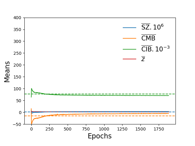
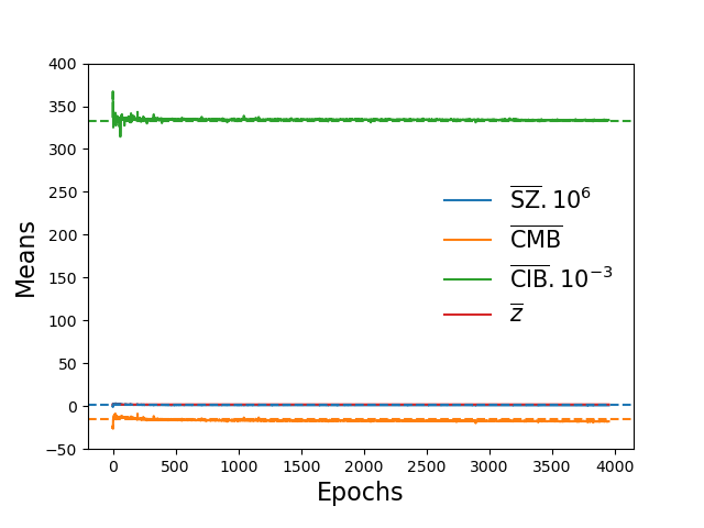
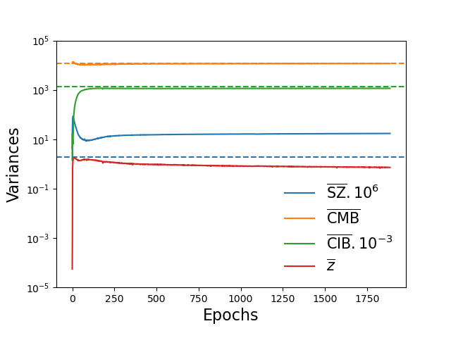
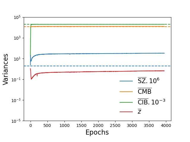
Figure 2: Evolution of the different statistical quantities of the extracted components in the unseen area of the sky. Top: evolution of the means of the components in the left for the 7 frequencies configuration and in the right for the 9 frequencies configuration. Bottom: evolution of the variances of the components in the left for the 7 frequencies configuration and in the right for the 9 frequencies configuration. Dotted lines represent the expected values. The values for the CIB are not the same for 7 and 9 frequencies as we are computing the 280 GHz one from the first case and the 545 GHz one for the second case. Units are different for each map: $\overline{\mathrm{SZ}}$ and $\overline{z}$ are without units ($y$ and redshift), $\overline{\mathrm{CMB}}$ is in $\mu\mathrm{K}$, and $\overline{\mathrm{CIB}}$ is in $\mathrm{MJy.sr}^{-1}$.

4.1 Frequency settings

First, we explore the impact of the choice of the frequency setting on the results and for this we have defined two combination of frequencies, one with seven frequencies, from 93 to 280 GHz, and another combination adding the 353 and 545 GHz frequency maps in which the CIB is dominant. We have compared the global properties of the components in the unseen area as a function of the epochs for the different combinations. The means and variances of the reconstructed components for the two frequency combinations are shown in Fig. 2. We directly see that the configuration with seven frequencies is not evolving into an expected solution (shown by the dotted lines), but rather shows biases in the mean values of all components and a lack of variance for the CIB. In the other configuration, the mean and variances are well recovered. This is due to the spectral dependencies of the SZ and the CIB in the range 100 - 250 GHz that are too similar, making it difficult to break the degeneracy between the two components. Instead of learning lower redshift $\overline{z}$ of the CIB at the position of the clusters as we expect (as CIB at the position of clusters is dominated by the galaxies from the galaxy clusters itself), it does an opposite effect and tends to learn higher redshift. This produces a lower bias in the SZ flux to balance the total emission and the model hence converges to an inaccurate solution. For these reasons, considering our model, we must take into account the higher frequencies maps at 353 and 545 where the CIB is dominant and where the spectral dependencies of the two components SZ and CIB start to differ one from another. In the following, our results are thus obtained in the configuration with nine frequencies including the 353 and 545 GHz maps. Also note that in Fig. 2, the values of the means and variances of the CIB are not the same for seven and nine frequencies, as we are computing the CIB at 280 GHz for the first case and the 545 GHz one for the second case.

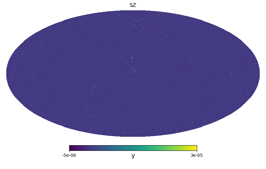
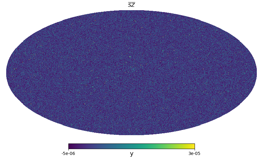
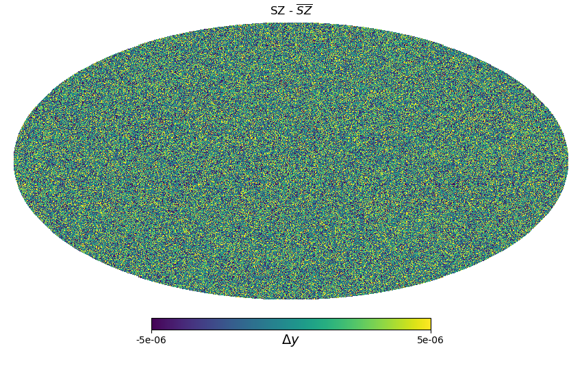
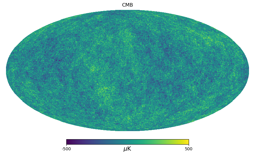
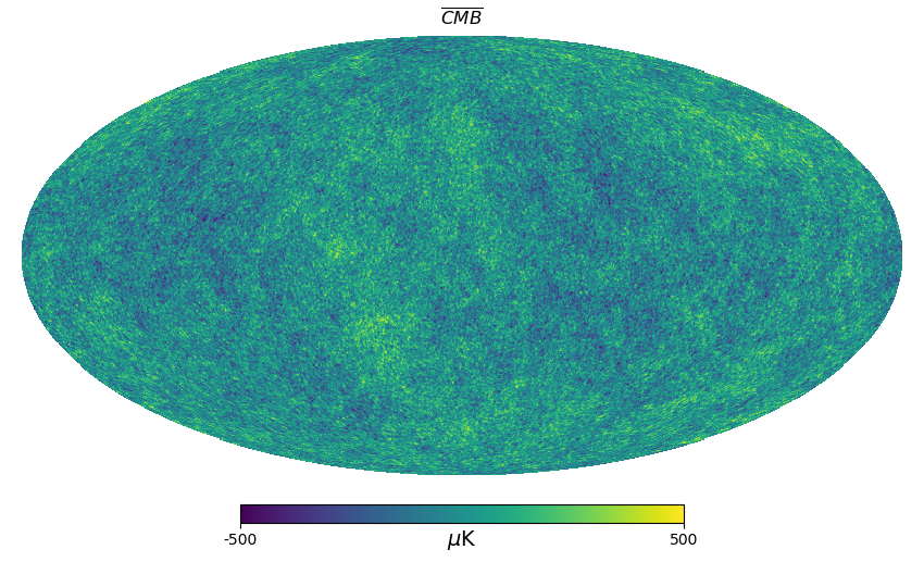
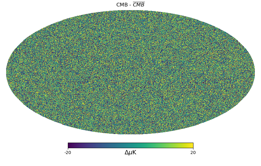
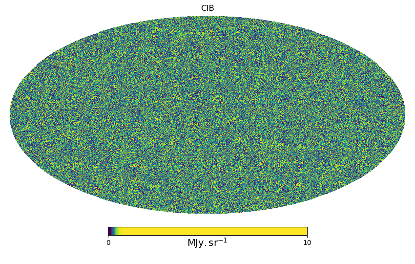
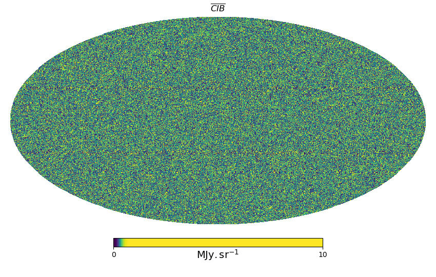
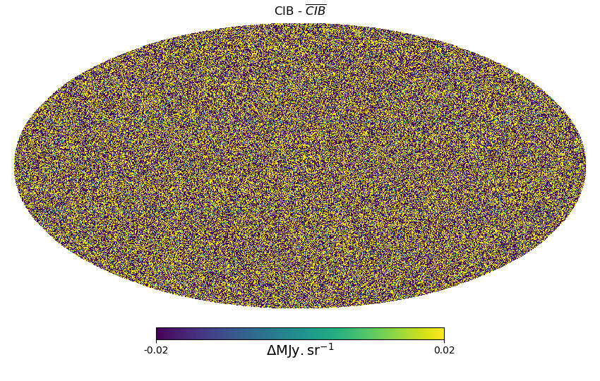
Figure 3: Mollweide projection of the full-sky HEALPIX maps of the different components. Left column: from top to bottom, the SZ, CMB, and CIB from WebSky simulation maps. Middle column: from top to bottom, the reconstructed $\overline{\mathrm{SZ}}$, $\overline{\mathrm{CMB}}$, and $\overline{\mathrm{CIB}}$. Right column: residuals between the Websky component and the reconstructed ones. A very good agreement is seen visually between the reconstructed maps and the expected one, without structures in the residuals.

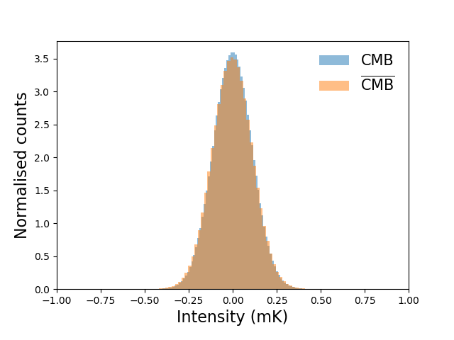
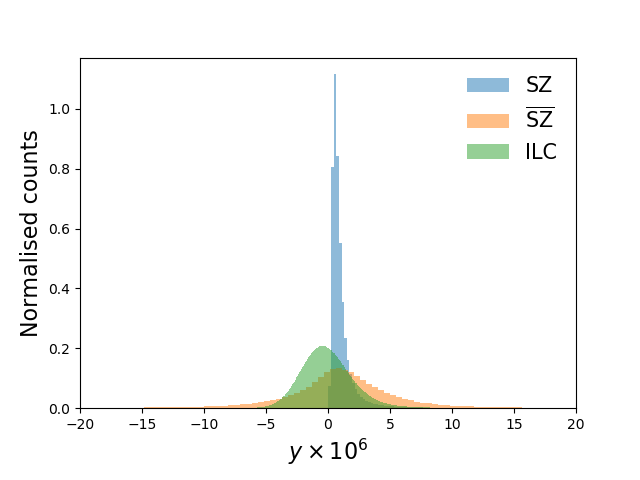
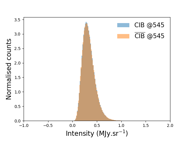
Figure 4: PDF comparison between the reconstructed components and the WebSky ones. Left: case for the CMB. Middle: case for the SZ. Right: case for the CIB.

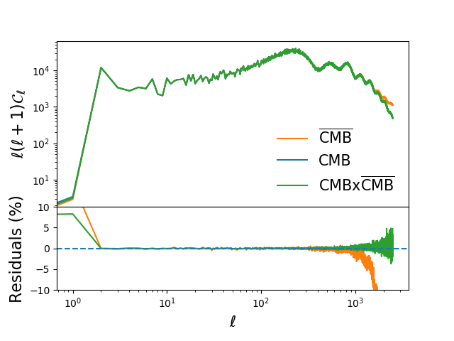
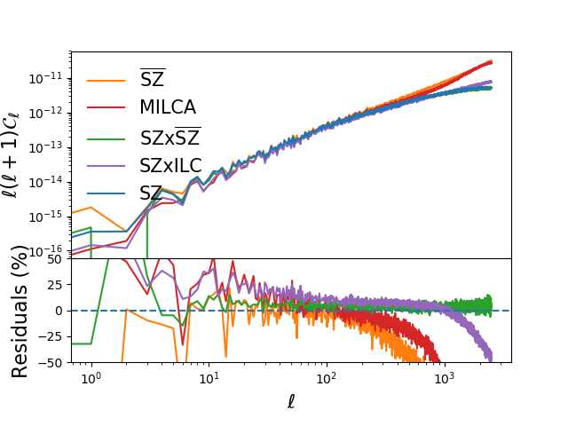
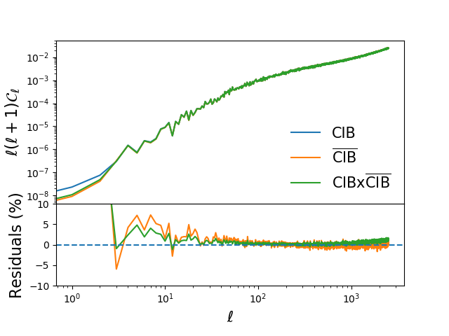
Figure 5: Power spectra of the components, the recovered components, and cross power spectra between the two. $\mathcal{C}_{\ell}$ residuals in percentage are also shown in the bottom of each plot. Left: case for the CMB. Middle: case for the SZ. MILCA is also shown in this plot. Right: case for the CIB.

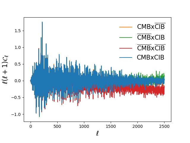
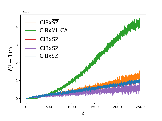
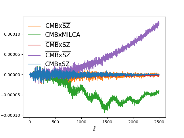
Figure 6: Cross power spectra between the different components. Left: case for CMBxCIB. Middle: case for CIBxSZ. MILCA is also considered in this plot. Right: case for CMBxSZ.

4.2 Visual inspection

We have trained our network with nine frequencies and reconstructed the HEALPIX maps of the four extracted components: $\overline{\mathrm{CMB}}$, $\overline{\mathrm{SZ}}$, $\overline{\mathrm{CIB}}$, and $\overline{z}$. The training lasted six days on a Tesla V100 GPU. A first comparison can be made visually to qualitatively check the ranges of pixel values, contrasts, and the non Gaussianity distribution of the pixels of the fields. In Fig. 3, we show Mollweide projections of $\overline{\mathrm{CMB}}$, $\overline{\mathrm{SZ}}$, and $\overline{\mathrm{CIB}}$ in the middle column, and we show in the left column the WebSky maps of CMB, SZ, and CIB. In the right column, we show the residuals between the reconstructed and true components. The reconstructed components seem visually in good agreement with the WebSky original components, without significant features seen in the residuals.

4.3 PDF comparison

We pursue our comparison by checking the PDF of the pixels for the different components. In Fig.4, we show the distribution of the pixels for the $\overline{\mathrm{CMB}}$, $\overline{\mathrm{SZ}}$, and $\overline{\mathrm{CIB}}$, where we compare to the original distributions from WebSky maps. For the case of SZ and CMB, we also compare to the distribution of pixels from the SZ maps reconstructed with MILCA. We see a very good match between the distributions of pixels for CMB and CIB, while the distribution is more flattened for the recovered SZ maps from our method and from MILCA. This indicates a noisy reconstruction of the SZ signal, that is expected considering the very low amplitude of the SZ effect compared to CMB or CIB that are the dominant signals in some frequencies. The reconstructed SZ map with our method seems however noisier than the one obtained with MILCA. This will be discussed further when we compare the cross-spectra and the contamination from other components.

4.4 Power spectra comparison

We have computed the auto power spectra for all the recovered components and compared them to the ones of the original WebSky components. For each component, we also compare the cross power spectra between the recovered components and the original ones, to check whether when removing the reconstructed noise of the estimated components, the signal is fully recovered. In Fig. 5, we show the resulting power spectra for the CMB in the left panel, SZ in the middle one, and CIB on the right. We also show the $\mathcal{C}_{\ell}$ residuals in percentage in the bottom of each plot. For the case of CMB, we recover very well the signal, with reconstructing noise dominating from $\ell>1000$. Removing the reconstructed noise in the cross spectrum with the WebSky CMB shows a very good recovery of the CMB signal, below 1% error up to $\ell=2500$. For the CIB, we have a very good agreement between the two power spectra, within 3% error and a bias below 2% up to $\ell=2500$. The cross spectrum between $\overline{\mathrm{CIB}}$ and CIB also shows a good recovery of the signal. For the SZ reconstructed maps (both for MILCA and for our method $\overline{\mathrm{SZ}}$), the power spectra are above the expected signal, especially at small scales. This indicates the presence of additional signal, e.g., noise, in good agreement with the effect seen in the distributions of the PDF in Sect. 4.3. By performing the cross spectra with the SZ WebSky map, interesting observations can be made. At small scales, $\ell>1000$, we see an excess of signal in the cross spectrum between MILCA and the true SZ emission from WebSKy (MILCAxSZ) leading to a bias of up to 50% at $\ell=2500$, that is not seen in the cross-spectrum $\overline{\mathrm{SZ}}$xSZ. This effect is due to the contamination of the CIB in the MILCA SZ map, that correlates with the SZ effect. The residuals of the cross-spectrum $\overline{\mathrm{SZ}}$xSZ indicate a good recovery of the signal within an error of 5% up to $\ell=2500$ and with a bias below 3% in all $\ell$. We will confirm this result in the next section, in which we compute the cross-spectra between all the components to study the contamination.

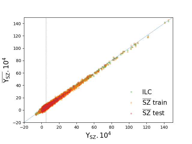
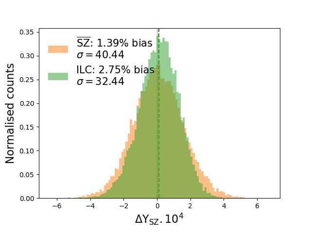
Figure 7: Comparison of the SZ fluxes computed with aperture photometry in the exact same way in the SZ WebSky map, in $\overline{\mathrm{SZ}}$ map, and in the MILCA SZ map. Left: fluxes on the reconstructed maps as a function of the SZ WebSky fluxes. The blue dashed line represents the flux limit for which clusters weight have been enhanced in the weight map $w$. Right: histograms of the residuals. The dashed lines show the median values of the distributions.

4.5 Cross-spectra between components

We have computed the cross-power spectra between all the components CMBxSZ, CMBxCIB, and CIBxSZ. In each case, we cross correlate all the combination between the original WebSky ones and the reconstructed ones, either from MILCA or with our method for the cases where SZ is involved. In Fig. 6, we show the results for all the different components. We detail hereafter the different cases.

4.5.1 CMBxCIB

For the case CMBxCIB (left panel of Fig. 6), where there is no correlation expected (blue line), we did not find any correlation between the different combinations, except for $\overline{\mathrm{CMB}}$x$\overline{\mathrm{CIB}}$. This means that the reconstructed CMB is not contaminated by the CIB, and that the reconstructed CIB is not contaminated by the CMB. On the other hand, the correlation between $\overline{\mathrm{CMB}}$ and $\overline{\mathrm{CIB}}$ is expected (but not necessarily problematic), as this correlation is coming from the correlated reconstructed noise between the two components, which is not expected to be independent as the two components are reconstructed at the same time.

4.5.2 CIBxSZ

For the case CIBxSZ (middle pannel of Fig. 6), there is an expected correlation between the two components (shown in blue) (Planck Collaboration, 2016; Stein et al., 2020). This correlation comes from the fact that the dominant part of the CIB in clusters, i.e. where the SZ signal is dominant, is generated from the dust emission of galaxies in this very same clusters. This correlation is a bias in the SZ reconstruction (e.g., Planck Collaboration, 2016) that we recover in $\overline{\mathrm{CIB}}$xSZ (in red), indicating that the reconstructed CIB is not contaminated by the SZ. However CIBxMILCA (in green) is above the correlation line, indicating that the MILCA SZ map is contaminated by CIB. This translates into an excess of SZ power at very small scales, that is also seen in the SZ auto power spectra in Sect.4.4. The cross-spectrum CIBx$\overline{\mathrm{SZ}}$ (in orange) is however much closer to the expected correlation in blue, indicating a tinier contamination from the CIB in the $\overline{\mathrm{SZ}}$ reconstructed map. The extra SZ power coming from CIB contamination is a potential source of bias for the study of the cosmological parameters from the SZ angular power spectrum (Komatsu & Seljak, 2002; Horowitz & Seljak, 2017; Douspis et al., 2022; Tanimura et al., 2022b), and is reduced in our method compared to MILCA.

4.5.3 CMBxSZ

For the case CMBxSZ (right panel of Fig. 6), no correlation is expected (blue line). We do not find any correlation neither with the recovered components, indicating that there is no contamination from CMB in the reconstructed SZ map, nor with the SZ in the reconstructed CMB map. In the SZ map derived with MILCA, we see an anti-correlation with the CMB, indicating a small contamination from the CMB in the SZ MILCA $y$ map.

4.6 SZ fluxes from clusters

After studying the statistics and contamination of the recovered component maps, we focus on the SZ fluxes from galaxy clusters. For each of the SZ maps, i.e., WebSky, MILCA, and $\overline{\mathrm{SZ}}$, we have computed in the exact same way, using aperture photometry, the SZ fluxes around a selection of the most massive low redshift clusters ($\mathrm{M}_{200}>4.10^{14}\mathrm{M}_{\odot}$ and $z<1$) from the numerical simulation (SZ fluxes for lower masses or higher redshift clusters become too low and noisy). We compare in Fig. 7 the SZ fluxes, in green from MILCA and in orange and red from $\overline{\mathrm{SZ}}$. The fluxes displayed in orange are obtained in the training region of the sky while the fluxes displayed in red are obtained in the unseen area of the sky. The very good consistency between all the fluxes indicate a very good recovery of the SZ fluxes for this selection of clusters with any methods, meaning that the network can recover well the SZ fluxes even in the unseen area, and with an error of the same order of magnitude than with the ones obtained with a state-of-the-art traditional methods such as MILCA. The dashed blue line in the figure indicates the flux limit for which the clusters have been enhanced in the weight-map $w$, used to re-balance the weight of the pixels inside clusters. We see a good correlation even before the vertical line, meaning that even clusters that have not been enhanced are very well recovered. This indicates that the weight-map $w$ is helping the network to learn faster the SZ spectral and spatial features but does not bias the results to the typical objects for which $w$ are input (otherwise, we would see a good agreement only beyond the vertical flux limit and no correlation before). In the right panel of Fig. 7 we compare the residuals of the SZ fluxes for MILCA and $\overline{\mathrm{SZ}}$. We see that the $\overline{\mathrm{SZ}}$ is a little bit noisier than MILCA, with a standard deviation of percentage residuals of $\sigma=40.4\%$ compare to $\sigma=32.4\%$ for MILCA, while the fluxes are a little bit less biased in the case of $\overline{\mathrm{SZ}}$, with a bias of 1.39% for $\overline{\mathrm{SZ}}$ and 2.75% in MILCA. Overall results tend to be similar for the two methods.

5 Discussion and summary

We have explored a new way of performing component separation using machine learning networks in a self-supervised way. Focused on the extragalactic submillimeter sky, this method allows us at the moment to extract a CMB, CIB, and SZ effect maps, and might already be applied to clean part of the sky (free from foreground emissions), for example to some of the cleanest regions (at very high galactic latitudes) of the Planck frequency maps. Being self-supervised, this method has the potential to be used directly to data without any need of known labeled data (the model that is trained here on numerical simulations will not be the one applied to real data). In this paper, we applied it to numerical simulations from WebSky and we achieved good results when we focused on the power spectra and cross spectra of the different reconstructed components, as well as interesting results regarding the contamination from the other components. Our method has still some limitations, that will be addressed in next studies. For example, we did not include any model of the foreground galactic emissions, i.e. dust, radio, CO sources. These emissions could be accounted for by adding in parallel other ResUNets allowing the reconstruction of these very same components all at once. We also did not include neither any models of noise nor of the effect of the instrumental beams as the aim of the paper was the theoretical response of these networks in an ideal case and the comparison with state-of-the-art methods (here MILCA). Focusing on the individual results for each component: for the case of CMB we achieve a very good reconstruction of the signal, although a bit noisy. When we cross-match with the CMB from WebSky, we achieve a very good reconstruction of the signal up to $\ell=2500$ at least. We obtain a very good reconstructed CIB, within a 3% error and a bias below 2% up to $\ell=2500$. For the SZ, we recover as well very nicely the signal, being less contaminated compared to the SZ map obtained with one of the state-of-the-art traditional methods, MILCA. None of the reconstructed components CMB or CIB are contaminated by other components as seen in the cross power spectra, and the contamination from CIB in the SZ reconstructed maps is lower than in MILCA as seen in Fig. 6. To remove completely the contamination of the CIB our spectral CIB model could be improved to take into account that the emission of the CIB is not a power-law but rather a sum of power-law that could be modeled in more details (for example in Taylor expansion, Chluba et al., 2017; Vacher et al., 2022b, a), but the modelling and the reconstruction of the CIB is a big challenge especially for the dust/CIB separation for the detection of the B-modes (e.g., Remazeilles et al., 2011; Remazeilles, 2018; Allys et al., 2019; Aylor et al., 2021; Regaldo-Saint Blancard et al., 2021). In Allys et al. (2019, 2020) for example, the authors have developed an algorithm similar to Convolutional Neural Networks based on Wavelet Scattering Transform (WST, Allys et al., 2019; Regaldo-Saint Blancard et al., 2020b) (main difference being that the filters of the layers of convolution are fixed instead of learned), to reproduce the statistics of the CIB and later input this statistic as a prior for the extraction of the CIB in component separation.

Compared to other method using deep learning network to extract components from CMB data (e.g., Caldeira et al., 2019; Grumitt et al., 2020; Li et al., 2022; Wang et al., 2022; Petroff et al., 2020; Lin et al., 2021), in our approach we estimate at the same time all components allowing a less-biased reconstruction of the dependencies, correlations, and contaminations with the other components (all components are dependent of each other during the training).

The lower effect of the CIB contamination in the power spectra especially on the SZ effect reconstruction could lead to less bias in the computation of the cosmological parameters using the SZ power spectra (Salvati et al., 2018; Douspis et al., 2022; Gorce et al., 2022; Tanimura et al., 2022b). Pushing even forward and modeling the polarisation, this method could in the future be used for the detection of the B-mode combining the data of Planck, ACT, SPT, SO (Ade et al., 2019), and CMB-S4 (Abazajian et al., 2019).