Supplemental Material for
99.92%-Fidelity CNOT Gates in Solids by Filtering Time-dependent and Quantum Noises

Diamond sample

The targeted NV center resides in a bulk diamond whose top face is perpendicular to the [100] crystal axis and lateral faces are perpendicular to the [110] axis. The bulk diamond is ultrapure with the nitrogen concentration less than 5 p.p.b., and the abundance of ¹³C atoms is at the natural level of 1.1$\%$. The diamond is irradiated using 10-MeV electrons to a total dose of $\sim$ 1.0 kgy. A solid immersion lens (SIL) is created around the targeted NV center to increase the luminescence rate of the NV to $\sim$ 300 kcounts/s.

Experimental setup

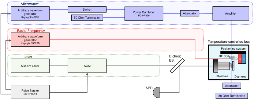
Figure S1: Simplified experimental setup. The setup mainly consists of microwave (blue) and radio-frequency (red) circuits, optical systems (green), synchronization system, and a diamond platform inside a temperature-controlled box.

The diamond is mounted on a typical confocal setup to perform optically detected magnetic resonance, synchronized with a microwave bridge by a multichannel pulse blaster (Spincore, PBESR-PRO-500). The 532-nm green laser for driving NV electron dynamics, and sideband fluorescence (650–800 nm) go through the same oil objective (Olympus, UPLSAPO 100XO, NA 1.40). To protect the NV center’s negative state and longitudinal relaxation time against laser leakage effects, all laser beams pass twice through acousto-optic modulators (AOM) (Gooch $\&$ Housego, power leakage ratio $\sim$ 1/1,000) before they enter the objective. The fluorescence photons are collected by avalanche photodiodes (APD) (Perkin Elmer, SPCM-AQRH-14) with a counter card (National Instruments, 6612). The 1.4 GHz and 4.3 GHz microwave (MW) pulses for manipulating three sublevels of the NV center are generated from an arbitrary waveform generator (AWG) (Keysight M8190), and fed into the coplanar waveguide microstructure. The 5.1 MHz radio-frequency (RF) pulses are generated from another AWG (Keysight 33522B), and applied for controlling the ¹⁴N nuclear spin through a RF coil. The external magnetic field ($\approx$ 510 G) is generated from a permanent magnet and aligned parallel to the NV axis through a three-dimensional positioning system. The positioning system, together with the platform holding the diamond and the objective, is placed inside a thermal insulation copper box. The temperature inside the copper box is stabilized at $\sim$ mK level through the feedback of the temperature controller (Stanford, PTC10). The overall setup is plotted in Fig. S1.

System Hamiltonian and noise Hamiltonian

The whole Hamiltonian for realizing the high-fidelity CNOT gate in this work, contains the terms concerning the system and the environmental noise.

$$H=H_{\text{sys}}+H_{\text{noi}}$$ (S1)

The system upon which the CNOT gate is performed, consists of the NV electron spin ($S=1$) and the ¹⁴N nuclear spin ($I=1$). A convention is made here that all physical quantities with the dimension of energy in the equations below are represented in the dimension of circular frequency, and their values are given in the dimension of frequency.

With an external magnetic field $B_{0}\approx$ 510 G applied along the axis of the NV center (defined as the $z$ axis), the system Hamiltonian is given by

$$H_{\text{sys}}=DS_{z}^{2}+\gamma_{e}B_{0}S_{z}+Q(I_{z}^{\text{N}})^{2}+\gamma_{\text{N}}B_{0}I_{z}^{\text{N}}+A_{\parallel}S_{z}I_{z}^{\text{N}}+A_{\perp}(S_{x}I_{x}^{\text{N}}+S_{y}I_{y}^{\text{N}})$$ (S2)

where $D=$ 2869.901 MHz are the zero-field splitting of the NV electron spin. $\gamma_{e}$ and $\gamma_{\text{N}}$ are the gyromagnetic ratios of the NV spin and the ¹⁴N spin, while $S_{x/y/z}$ and $I_{x/y/z}^{\text{N}}$ denote the $x/y/z$ components of the spin operators for two spins. By means of the method in the work [1], the ¹⁴N quadrupole coupling $Q$, the parallel component $A_{\parallel}$, the transverse component $A_{\perp}$ of the hyperfine interaction, and the ratio $\gamma_{e}/\gamma_{\text{N}}$ are given by -4945.8003(12) kHz, -2164.6714(17) kHz, -2632.8(8) kHz, and -9113.77(8), respectively. As described in the text, the system is disturbed by interactions with $N$ ¹³C nuclear spins

$$H_{\text{noi}}^{N}=\sum_{i=1}^{N}\gamma_{\text{C}}B_{0}I_{z}^{i}+S_{z}(A_{zx}^{i}I_{x}^{i}+A_{zy}^{i}I_{y}^{i}+A_{zz}^{i}I_{z}^{i})$$ (S3)

where the ¹³C Larmor frequency $\omega_{\text{C}}=\gamma_{\text{C}}B_{0}\approx$ -546.67 kHz. Since the hyperfine interactions are weak enough, Eq. (S3) excludes non-secular coupling terms, which mix the states of the NV electron spin and thus are negligible here. In the interaction picture of the ¹³C spin precession, the noise Hamiltonian becomes time-dependent

$$H_{\text{noi}}^{N}(t)= \left(\cos(\omega_{\text{C}}t)\sum_{i=1}^{N}(A_{zx}^{i}I_{x}^{i}+A_{zy}^{i}I_{y}^{i})+\sin(\omega_{\text{C}}t)\sum_{i=1}^{N}(A_{zx}^{i}I_{y}^{i}-A_{zy}^{i}I_{x}^{i})\right)S_{z}$$ (S4)

$$+S_{z}\sum_{i=1}^{N}A_{zz}^{i}I_{z}^{i}$$

In the weak coupling limit, the overall effect of a great number of ¹³C spins is like classical noise, and that is, three sums in Eq. (S4) become three Gaussian distributions based on the central limit theorem. Therefore, apart from the proximal five ¹³C spins detected by DD sequences as shown in Fig. 1(b) of the main text, the other ¹³C spins can be taken as a whole classical noise. By replacing the sums of Eq. (S4) with three Gaussian random variables $X$, $Y$, and $Z$, the ¹³C spin bath is modelled by

$$H_{\text{noi}}(t)=(X\cos(\omega_{\text{C}}t)+Y\sin(\omega_{\text{C}}t)+Z)S_{z}+H_{\text{noi}}^{5}$$ (S5)

where $H_{\text{noi}}^{5}$ is the Hamiltonian of the five ¹³C spins in the Schrödinger picture, given by Eq. (S3). The time-dependent part $X\cos(\omega_{\text{C}}t)+Y\sin(\omega_{\text{C}}t)$ in Eq. (S5) is exactly the time-varying noise $\eta(t)$ used in the main text, while $Z$ represents the static noise. In this work, the gate error induced by the ¹³C spin bath is estimated based on the model above, but the numerical optimization of the shaped pulse for acquiring the high-fidelity CNOT gate takes the five¹³C spins as classical as well, as stated in the main text. It can be inferred from the deduction above that the noise model used here is close enough to the real noise environment.

After abandoning the spin state $|{m_{\scaleto{S}{4.5pt}}=+1\rangle}$ of the NV electron spin and the state $|{m_{\scaleto{I}{4.5pt}}=-1\rangle}$ of the ¹⁴N nuclear spin, the left four levels comprise the two qubits used for realizing the CNOT gate, as shown in Fig. 3(a) of the main text. The system Hamiltonian in Eq. (S2) reduced to the four-level subspace after removing some constant terms is given by

$$H_{\text{sys}}=\omega_{\scaleto{S}{4.5pt}}S_{z}+\omega_{\text{N}}I_{z}^{\text{N}}+A_{\parallel}S_{z}I_{z}^{\text{N}}$$ (S6)

where $S_{z}$ and $I_{z}^{\text{N}}$ are changed into the spin-1/2 operators for two spins, and $\omega_{\scaleto{S}{4.5pt}}$ and $\omega_{\text{N}}$ are the transition frequencies of two spins. The coupling term $A_{\parallel}$ is adjusted to be 2159.876 kHz for the four levels above resulting from the second perturbative effect of the transverse component $A_{\perp}$. Accordingly, the form of the hyperfine interactions with the surrounding ¹³C spins needs to be changed, especially for $H_{\text{noi}}^{5}$ in the noise model above

$$H_{\text{noi}}^{5} =\sum_{i=1}^{5}\omega_{\text{C}}I_{z}^{i}+(S_{z}-\frac{\mathbb{I}}{2})(A_{zx}^{i}I_{x}^{i}+A_{zy}^{i}I_{y}^{i}+A_{zz}^{i}I_{z}^{i})$$ (S7)

$$\approx\sum_{i=1}^{5}\omega_{\text{C}}^{i}I_{z}^{i}+S_{z}(A_{zx}^{i}I_{x}^{i}+A_{zy}^{i}I_{y}^{i}+A_{zz}^{i}I_{z}^{i})$$

where $\omega_{\text{C}}^{i}=\omega_{\text{C}}-A_{zz}^{i}/2$. The second line in Eq. (S7) abandons the terms $-A_{zx}^{i}I_{x}^{i}/2$ and $-A_{zy}^{i}I_{y}^{i}/2$, since $A_{zx}^{i}$ and $A_{zy}^{i}$ are much smaller than $\omega_{\text{C}}$. For the strongly coupled ¹³C spins, their precession frequencies are slightly changed by the hyperfine interactions with the NV center, which explains the shifted noise peaks of the five ¹³C spins in Fig. 1(c) and Fig. 2(b) of the main text.

As described in Fig. 3(a), the MW pulse is resonantly applied in the nuclear state $m_{\scaleto{I}{4.5pt}}=0$ with the frequency $\omega_{\text{MW}}=\omega_{\scaleto{S}{4.5pt}}-A_{\parallel}/2$. Taking the interaction picture with respect to $\omega_{\text{MW}}S_{z}$ and $(\omega_{\text{N}}-\omega_{\text{sh}})I_{z}$, the system Hamiltonian reads

$$H_{\text{sys}}^{\text{int}}=A_{\parallel}S_{z}(I_{z}^{\text{N}}+\frac{\mathbb{I}}{2})+\omega_{\text{sh}}(I_{z}^{\text{N}}-\frac{\mathbb{I}}{2})$$ (S8)

where $\omega_{\text{sh}}=1/(4T_{\text{CNOT}})$ with $T_{\text{CNOT}}$ denoting the duration of the realized CNOT gate. The constant term $-\omega_{\text{sh}}\mathbb{I}/2$ is added to compensate for the negative determinant of the CNOT gate. In the same picture, according to rotating wave approximtaion (RWA), the non-resonant component of the applied MW is abandoned. The Hamiltonian obtained for MW control is written as

$$H_{\text{c}}(t)=\Omega_{\text{r}}(t)S_{x}+\Omega_{\text{i}}(t)S_{y}$$ (S9)

with arbitrarily adjustable $\Omega_{\text{r}}(t)$ and $\Omega_{\text{i}}(t)$ by time-dependently setting the amplitude and phase of the MW pulse generated by the AWG. The control Hamiltonian of Eq. (S9) together with the system Hamiltonian of Eq. (S8) is used for generating the strictly defined CNOT gate under the noise model of Eq. (S5) by using $H_{\text{noi}}^{5}$ in Eq. (S7). The approximations in the derivation above, such as the reduction of the system Hamiltonian (population leakage) and RWA, are considered in the gate error analysis, while the approximations concerning the interactions with the ¹³C reservoir, at most, cause a small deviation in estimating the error from the ¹³C spin bath.

Experimental construction of the noise model

All parameters in the noise model described by Eq. (S5) are determined experimentally. First of all, the coupling parameters of the nearby five ¹³C spins are obtained by adopting the method in the work [2]. The DD sequences in Fig. 1(b) and Fig. S2 are applied between the spin state $|{m_{\scaleto{S}{4.5pt}}=0\rangle}$ and the state ${|m_{\scaleto{S}{4.5pt}}=+1\rangle}$ with the $\pi$ pulse interval $\tau$. It is assumed that a ¹³C spin coupled to the NV center has the coupling parameters $(A_{zx},A_{zy},A_{zz})$ as in Eq. (S3). If the NV spin stays in the state $|{m_{\scaleto{S}{4.5pt}}=0\rangle}$, the ¹³C spin feels the same field as the external field with the transition frequency $\omega_{0}=\omega_{\text{C}}$ and the direction denoted by $\hat{\mathbf{n}}_{0}$; if the NV spin stays in the state $|{m_{\scaleto{S}{4.5pt}}=+1\rangle}$, the ¹³C spin is influenced by both the external field and the hyperfine interation, giving the resulting frequency $\omega_{1}=\sqrt{A_{zx}^{2}+A_{zy}^{2}+(\omega_{\text{C}}+A_{zz})^{2}}$ and the direction $\hat{\mathbf{n}}_{1}$. After some algebraic calculation, the decoherence of the NV spin may be caused by the non-parallelism between $\hat{\mathbf{n}}_{0}$ and $\hat{\mathbf{n}}_{1}$ with $|\hat{\mathbf{n}}_{0}\cdot\hat{\mathbf{n}}_{1}|<1$

$$C(\tau)=1-2\left(1-(\hat{\mathbf{n}}_{0}\cdot\hat{\mathbf{n}}_{1})^{2}\right)\sin^{2}(\frac{\omega_{0}\tau}{4})\sin^{2}(\frac{\omega_{1}\tau}{4})\frac{\sin^{2}(\frac{N\phi(\tau)}{2})}{\cos^{2}(\frac{\phi(\tau)}{2})}$$ (S10)

with

$$\cos(\phi(\tau))=\cos(\frac{\omega_{0}\tau}{2})\cos(\frac{\omega_{1}\tau}{2})-\hat{\mathbf{n}}_{0}\cdot\hat{\mathbf{n}}_{1}\sin(\frac{\omega_{0}\tau}{2})\sin(\frac{\omega_{1}\tau}{2})$$ (S11)

The decoherence dip caused by the ¹³C spin will emerge repeatedly when the interval $\tau$ is equal to

$$\tau_{k}=\frac{(2k-1)\pi}{(\omega_{0}+\omega_{1})/2}$$ (S12)

with the resonance order $k$. According to the behavior of DD filter function [3, 4], a larger $\tau$ leads to a better spectral resolution, and thus a larger $k$ is preferred. The order $k=$ 9 is chosen to clearly distinguish the five ¹³C spins, as displayed in Fig. 1(b) of the main text. The coupling parameters are extracted by data fitting using Eq. (S10) with suitable orders $k$ for each ¹³C spin as shown in Fig. S2(b-e). The fitting results give the values of $A_{zz}$ and $\sqrt{A_{zx}^{2}+A_{zy}^{2}}$, all gathered in the table of Fig. 1(c). It is not necessary to obtain the values of $A_{zx}$ and $A_{zy}$ for the error analysis of the CNOT gate, and thus an angle $\phi$ is arbitrarily chosen to assign these two values.

The other ¹³C spins are indistinguishable by DD sequences at room temperature, and thus treated as classical noise. Actually, the nearby five ¹³C spins can be taken as classical noise as well, because as described in the main text, they are not included in the numerical optimization but the shaped pulse optimized still bears the ability to disentangle with these ¹³C spins. From this aspect, it is justified that the other ¹³C spins are taken as a whole classical noise containing static and time-varying components. In the following, the strengths of the static noise and the time-varying noise, i.e., the standard deviations of three zero-mean Gaussian random variables $X$, $Y$, and $Z$ in Eq. (S5), are both determined. As shown in Fig. S3(a), the NV coherence is measured under a Ramsey sequence. An exponential fit with the function $a\cos(2\pi(\delta f)t+\phi_{0})e^{-(t/T_{2}^{*})^{p}}+b$ can not explain the last few points very well, which manifests the signatures of the nearby five ¹³C spins. The contribution of the five ¹³C spins under the Ramsey sequence is numerically calculated and deducted from Fig. S3(a), giving the results in Fig. S3(b). Thus, the decoherence from the weakly coupled ¹³C spins is obtained. Since the effect of the time-varying noise is negligible for the NV coherence under the Ramsey sequence, the strength of the static noise is extracted to be $\sigma=$ 20.0(1.5) kHz by fitting with the function $e^{-(2\pi\sigma t)^{2}/2}$. As for the time-varying noise, the strengths of two quadrature amplitudes $X$ and $Y$ are determined by comprehensively considering the simulation of the dip indicated by the label “¹³C Bath” in Fig. 1(b) of the main text and the gate fidelities calculated for the primitive gate and the shaped pulse with only static-noise resistance. It is known from Eq. (S4) that both random variables must have the same standard deviation, i.e., $\sigma_{x}=\sigma_{y}$. When the strengths $\sigma_{x}$ and $\sigma_{y}$ take the value of 30 kHz, the calculated fidelities for these two gates are 99.46% and 98.26%, agreeing well with the experimentally measured values 99.52(2)% and 98.27(6)% in the main text, and at the same time, the dip described above can be explained well by the simulation as shown in Fig. S3(c).

In summary, all parameters in the noise model used in this work are determined by performing multiple experiments, consisting of the proximal five ¹³C spins with the coupling parameters listed in the table of Fig. 1(c), the static noise with the strength of 20 kHz and the time-varying noise with the strength of 30 kHz. The noise model is employed to estimate the gate error from the ¹³C spin bath and optimize the shaped pulse after transforming the five ¹³C spins into the corresponding static and time-varying noises.

Optimization of shaped pulses

Considering the high computational overhead demanded for simulating five quantum objects (¹³C spins), the noise model used for the optimization of shaped pulses has to be simplified at first. The five ¹³C spins are classicized in the manner of taking $A_{zz}/2$ as the strength of a static noise, and $\sqrt{A_{zx}^{2}+A_{zy}^{2}}/2$ as the combined strength $\sqrt{\sigma_{x}^{2}+\sigma_{y}^{2}}$ of a time-varying noise. The combined strength for each ¹³C spin is exactly the area of the corresponding peak in the noise spectrum of the five ¹³C spins as displayed in Fig. 1(c) of the main text. With the processing method above, the noise from the ¹³C spin bath is totally classical and has the form

$$H_{\text{noi}}^{\text{opt}}(t)=(X^{\text{opt}}\cos(\omega_{\text{C}}t)+Y^{\text{opt}}\sin(\omega_{\text{C}}t)+Z^{\text{opt}})S_{z}$$ (S13)

which is totally determined by new random variables $X^{\text{opt}}$, $Y^{\text{opt}}$, and $Z^{\text{opt}}$. Combined with the noise contributions from the weakly coupled ¹³C spins, the strengths of these random variables are given by 45.4 kHz, 45.4 kHz, and 53.4 kHz, respectively.

Combined with the system Hamiltonian of Eq. (S8) and the control Hamiltonian of Eq. (S9), the unitary operation realized by a shaped pulse under a noise sample $x_{i}^{\text{opt}}$, $y_{i}^{\text{opt}}$, and $z_{i}^{\text{opt}}$, can be written as

$$U_{i}=\mathcal{T}e^{-i\int_{0}^{T_{\text{CNOT}}}(H_{\text{sys}}^{\text{int}}+H_{\text{c}}(t)+H_{i}^{\text{opt}}(t))dt}$$ (S14)

where $\mathcal{T}$ is the time ordering operator in that the integrand Hamiltonian is time-dependent. The noise Hamiltonian $H_{i}^{\text{opt}}(t)$ under the noise sample takes the form of $H_{i}^{\text{opt}}(t)=(x_{i}^{\text{opt}}\cos(\omega_{\text{C}}t)+y_{i}^{\text{opt}}\sin(\omega_{\text{C}}t)+z_{i}^{\text{opt}})S_{z}$. The overall goal of the optimization is, by repeatedly adjusting the time-varying amplitudes $\Omega_{\text{r}}(t)$ and $\Omega_{\text{i}}(t)$ of the shaped pulse, to maximize the gate fidelity under $M$ noise samples

$$\mathcal{F}_{\text{CNOT}}^{\text{opt}}=\frac{1}{M}\sum_{i=1}^{M}\left|\text{Tr}(U_{\text{CNOT}}^{\dagger}U_{i})/4\right|^{2}$$ (S15)

where $U_{\text{CNOT}}$ is the ideal CNOT gate, and Tr obtains the trace of a matrix. The optimization algorithm adopted here is a gradient-based algorithm, i.e., the gradient ascent pulse engineering (GRAPE) algorithm [5]. Before implementing the algorithm, for the sake of lowering the computational overhead, we let the shaped pulse take a piecewise-constant profile with the initial values randomly generated. As shown in Fig. 4(a) of the main text, the shaped pulse has 30 pieces for both real and imaginary parts (60 in total) with each piece lasting for 50 ns. Besides, it is noteworthy that only a few points are needed in the noise sampling, and (-88, 0, 88 kHz) for the static noise $Z^{\text{opt}}$ and (-76, 0, 76 kHz) for the time-varying noise $X^{\text{opt}}$ and $Y^{\text{opt}}$ are employed here for a larger noise tolerance.

Universality of our method

Because the coupling parameters of the ¹³C spins are not involved in the optimization above, the optimized shaped pulse also applies to the other NV centers without very strongly coupled ¹³C spins (e.g., $\sim$ MHz). An alternative noise sampling with a strength of up to 150 kHz is also feasible for a better noise tolerance, which is sufficient for the NV center in the diamond with a natural abundance of ¹³C atoms. For the NV center with $\sim$ MHz coupled ¹³C spins, the ¹³C spins must be treated as quantum objects and included in the system Hamiltonian in the optimization process. In general, such $\sim$ MHz coupled ¹³C spins are often few, one or two if any, and thus will not dramatically increase the computational overhead even though they are treated as quantum objects in the optimization.

Performance of the optimized shaped pulse

The shaped pulse is elaborately designed for realizing a high-fidelity CNOT gate with the optimization method introduced above. By numerically simulating the gate realized by the shaped pulse under the complete noise model (the five ¹³C spins, the static noise (20 kHz), and the time-varying noise (30 kHz)), the gate error from the ¹³C spin bath is estimated to be 0.074‰ (Fig. 4(d)).

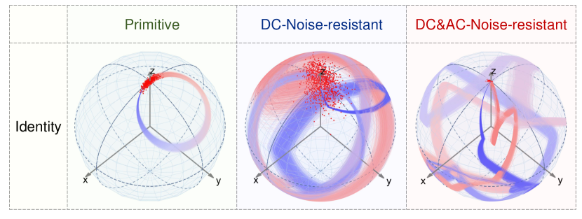
Figure S4: Resistance to time-dependent noise. The state evolutions under the Identity operation of the CNOT gate for three kinds of control pulses are calculated with 1000 samples of the time-varying noise described in the main text. The results are exhibited on the Bloch sphere. See the NOT part of the CNOT gate in Fig. 2(c) of the main text.

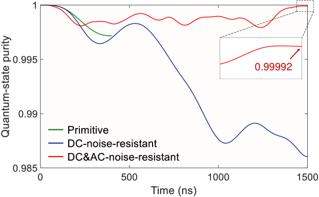
Figure S5: Resistance to quantum noise. The quantum-state purity under the Identity operation of the CNOT gate is numerically calculated for comparing the abilities of three kinds of control pulses to resist the quantum noise caused by the proximal five ¹³C spins. See the NOT part of the CNOT gate in Fig. 2(e) of the main text.

Furthermore, the abilities of the shaped pulse to resist classical noise and quantum noise can be investigated separately. The performance of resisting classical noise is manifested by calculating the gate errors under time-varying noises $\eta(t)=X^{\prime}\cos(\omega t)+Y^{\prime}\sin(\omega t)$ with different frequencies $\omega$ (Fig. 2(a)). The random variables $X^{\prime}$ and $Y^{\prime}$ are zero-mean Gaussian distributions with the standard deviations given by $\sigma_{x}=\sigma_{y}=$ 70 kHz. The noise strength chosen here is a little larger than that of the fully classicized ¹³C spin bath (45.4 kHz) for demonstrating a better noise tolerance than demanded. The state evolutions under the shaped pulse are calculated with 1000 noise samples at the ¹³C Larmor frequency, as displayed in Fig. 2(a) (the NOT operation) and Fig. S4 (the Identity operation), together with the primitive gate and the shaped pulse with only static-noise resistance for comparison. The ability to resist quantum noise is embodied by calculating the quantum-state purity under the unitary evolution with the system Hamiltonian including the nearby five ¹³C spins, as displayed in Fig. 2(e) (the NOT operation) and Fig. S5 (the Identity operation), together with the other two pulses for comparison.

Subspace randomized benchmarking

It is an intrinsic problem for a hybrid system to directly perform two-qubit RB sequences, due to the vast difference in the quantum control for different quantum objects (here the electron spin and the nuclear spin). Fortunately, the two-qubit RB can be simplified to be performed in subspaces under some reasonable approximations, called subspace randomized benchmarking (SRB) [6]. The deviation arising therefrom is smaller than that of IRB [7], which is verified here by numerical simulation.

The gate fidelity is generally defined as the state fidelity averaged over the whole state space

$$\mathcal{F}_{U}=\int_{|\psi\rangle}\langle\psi|U^{\dagger}\Lambda_{U}(|\psi\rangle\langle\psi|)U|\psi\rangle d\psi$$ (S16)

where $U$ is the target gate and $\Lambda_{U}$ is the quantum operation close to $U$. The target gate here is the CNOT gate $U_{\text{CNOT}}$. The gate realized by the optimized shaped pulse is indeed a quantum operation performed upon the two-spin system, resulting from unwanted entanglement with the ¹³C spin bath, as shown in Fig. 2(e) and Fig. S5. Therefore, when the ¹³C spin bath is considered as part of the system Hamiltonian, the whole operation will be unitary

$$\Lambda_{\text{CNOT}}(|\psi\rangle\langle\psi|) =\text{Tr}_{\text{bath}}\left(U_{\text{CNOT}}^{\text{exp}}(|\psi\rangle\langle\psi|\otimes\rho_{\text{bath}})(U_{\text{CNOT}}^{\text{exp}})^{\dagger}\right)$$ (S17)

$$=\frac{1}{d_{\text{bath}}}\sum_{i,j}\langle\psi_{\text{bath}}^{i}|U(|\psi\rangle|\psi_{\text{bath}}^{j}\rangle\langle\psi_{\text{bath}}^{j}|\langle\psi|)(U_{\text{CNOT}}^{\text{exp}})^{\dagger}|\psi_{\text{bath}}^{i}\rangle$$

where $U_{\text{CNOT}}^{\text{exp}}$ is the CNOT gate realized experimentally in the whole Hilbert space. The $U_{\text{CNOT}}^{\text{exp}}$ is obtained under the interaction picture of the Larmor precession for each ¹³C spin so that the effect on the ¹³C spin bath is nearly the Identity operation. The bath state $\rho_{\text{bath}}$ is the maximum mixed state $\frac{1}{d_{\text{bath}}}\sum_{j}|\psi_{\text{bath}}^{j}\rangle\langle\psi_{\text{bath}}^{j}|$. In Eq. (S17), the ensemble average of the MW pulse fluctuation is ignored for simplicity considering that the error arising therefrom is rather small as shown in Fig. 4(d) of the main text. The longitudinal relaxation of the electron spin is also ignored here in that it is a depolarized channel compatible with the RB [8]. Substituting Eq. (S17) into Eq. (S16) gives the fidelity of the CNOT gate

$$\mathcal{F}_{\text{CNOT}} =\frac{1}{d_{\text{bath}}}\sum_{i,j}\int_{|\psi\rangle}\left|\langle\psi_{\text{bath}}^{i}|\langle\psi|U_{\text{CNOT}}^{\dagger}U_{\text{CNOT}}^{\text{exp}}|\psi\rangle|\psi_{\text{bath}}^{j}\rangle\right|^{2}d\psi$$ (S18)

$$\approx\frac{1}{(4d_{\text{bath}})^{2}}\left|\text{Tr}(U_{\text{CNOT}}^{\dagger}U_{\text{CNOT}}^{\text{exp}})\right|^{2}$$

where the ideal CNOT gate $U_{\text{CNOT}}$ is also extended into the whole Hilbert space with the Identity operation on the ¹³C spin bath. The approximation in Eq. (S18) holds well [9], which is verified by numerical calculation by taking the five ¹³C spin into consideration. The gate fidelity is expressed exactly as that used in the optimization with Eq. (S15) except the noise average. With Eq. (S18), the fidelity of the CNOT can be divided as

$$\mathcal{F}_{\text{CNOT}} =\frac{1}{(4d_{\text{bath}})^{2}}\left|\text{Tr}(U_{\text{Ide}}^{\dagger}U_{\text{Ide}}^{\text{exp}})+\text{Tr}(U_{\text{NOT}}^{\dagger}U_{\text{NOT}}^{\text{exp}})\right|^{2}$$ (S19)

$$\approx\frac{1}{4}\left(\frac{1}{2d_{\text{bath}}}\left|\text{Tr}(U_{\text{Ide}}^{\dagger}U_{\text{Ide}}^{\text{exp}})\right|+\frac{1}{2d_{\text{bath}}}\left|\text{Tr}(U_{\text{NOT}}^{\dagger}U_{\text{NOT}}^{\text{exp}})\right|\right)^{2}$$

$$=\frac{1}{4}(\sqrt{\mathcal{F}_{\text{Ide}}}+\sqrt{\mathcal{F}_{\text{NOT}}})^{2}$$

Based on the equation above, the fidelity of the CNOT gate can be obtained by separately measuring the fidelities of the Identity operation and the NOT operation. The approximation in Eq. (S19) is made by ignoring the error from the nuclear-spin decoherence, which gives an estimated error of $7\times 10^{-6}$ in Fig. 4(d) of the main text.

Experimental implementation of randomized benchmarking

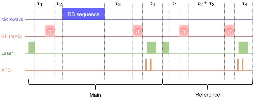
Figure S8: Experimental sequence for applying randomized benchmarking. The reference sequence is nearly identical to the main sequence except the absence of the RB sequence. The RF pulses are only used for measuring the gate fidelity in the $m_{\scaleto{I}{4.5pt}}=0$ subspace.

The two-qubit system used in this work consists of the NV electron spin and the ¹⁴N nuclear spin. It can be collectively initialized into the state $|{m_{\scaleto{S}{4.5pt}}=0}\rangle|{m_{\scaleto{I}{4.5pt}}=+1}\rangle$ by a 532-nm laser pulse under a magnetic field of about 510 G, and the population of the state $|m_{\scaleto{S}{4.5pt}}=0\rangle$ can be read out by collecting fluorescence photons. The experimental sequence for implementing randomized benchmarking (RB) is plotted in Fig. S8. Apart from the main sequence for performing the RB sequence, a reference sequence is also indispensable and nearly identical to the main sequence except the absence of the RB sequence. After running the sequence, the obtained result is the ratio of the numbers of the collected photons from the main sequence, and after normalization by Rabi oscillations, the population of $|{m_{\scaleto{S}{4.5pt}}=0}\rangle$ for the fidelity measurement is obtained.

Before the fidelity measurement, the population is guaranteed to be 1 within the errorbar when the RB sequence is applied with a large detuning. The unit population is reasonable since the mixed part of the state is removed after normalization by Rabi oscillations, and does not indicate that the initial state is pure enough. The verification above eliminates varieties of unwanted disturbances affecting the results of the fidelity measurement, such as the laser power fluctuation, the drift of the NV position, the heating effect, and so on. Among them, the heating effect mainly originated from the RB sequence is especially noteworthy. The heat-expansion can drift the position of the NV center and then decrease the counting rate, which may lead to inaccurate results of the fidelity measurement. Therefore, the heating effect is measured with the results for the single-qubit RB and the IRB for the CNOT gate displayed in Fig. S9(a), both of which are negligible within the errorbars. The results above also indicate that all other disturbances do not affect the fidelity measurement. The sequence for measuring the heating effect (Fig. S9(b)) is similar to the sequence of Fig. S8, except that the RB sequence is off-resonant by 1 GHz and the idle stage of the reference sequence includes the duration of the RB sequence.

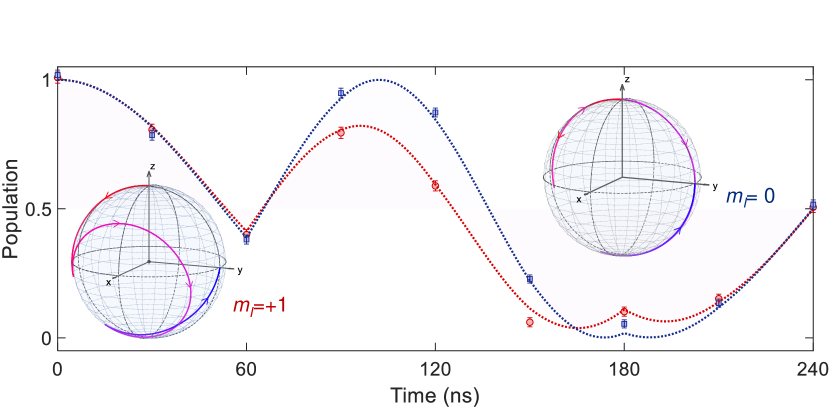
Figure S6: Measured evolutions for two nuclear states under the $\pi/2$ gate. The $\pi/2$ gate is realized by applying the shaped pulse in Fig. 3(b) of the main text. The solid lines are the results of the theoretical simulation. The evolutionary trajectories on the Bloch sphere are also exhibited for a visual comparison.

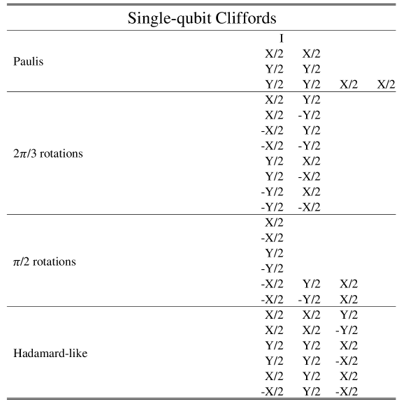
Figure S7: Single-qubit Cliffords. The Single-qubit Clifford group contains 24 gates in total, and all can be generated by the $\pi/2$ gate with the shaped pulse in Fig. 3(b) of the main text.

Before benchmarking the CNOT gate with the SRB method described above, the performance of single-qubit gates needs to be characterized first. The state evolutions in both nuclear subspaces under the $\pi/2$ gate are measured, in a good agreement with the numerical calculation as shown in Fig. S6. Since the error of an individual $\pi/2$ gate is too small to be covered by the readout noise, the method of RB has to be adopted to enlarge the error by randomly concatenating many Clifford gates. With the table of Fig. S7, all single-qubit Cliffords can be built from the basic block, i.e., the $\pi/2$ gate realized by the shaped pulse in Fig. 3(b) of the main text. Each Clifford gate contains $13/6$ gates on the average. The $\pi/2$ gate here is a true single-qubit gate that implements the same operation in both nuclear subspaces, rather than only working in the $m_{\scaleto{I}{4.5pt}}=+1$ as done by the previous work [10]. When the RB sequence is carried out in the $m_{\scaleto{I}{4.5pt}}{=+1}$ subspace, a RF $\pi$ pulse for driving the transition $|{m_{\scaleto{S}{4.5pt}}=0}\rangle|{m_{\scaleto{I}{4.5pt}}=+1}\rangle\leftrightarrow|{m_{\scaleto{S}{4.5pt}}=0}\rangle|{m_{\scaleto{I}{4.5pt}}=0}\rangle$ is applied before and after the RB sequence to prepare and readout the population of the state $|{m_{\scaleto{S}{4.5pt}}=0}\rangle|{m_{\scaleto{I}{4.5pt}}=+1}\rangle$. The single-qubit RB and the SRB for evaluating the CNOT gate are executed in both nuclear subspaces with the results described in the main text.

Gate error analysis

Although the error from the reservoir is largely suppressed by the DEC effect of the shaped pulse, the errors from the longitudinal relaxation of the electron spin and the waveform distortion of the shaped pulse become more significant, due to a more complicated pulse composition and a longer gate time compared with the primitive gate. Apart from the two most important factors, all error sources are detailedly analyzed here, except the error from ¹³C spin bath discussed above, with the results summarized in the table of Fig. 4(d).

First of all, longitudinal relaxation behaviors of the NV spin triplet are measured for estimating the error arising therefrom. When the initial state is prepared at the eigenstates $m_{\scaleto{S}{4.5pt}}=0,\pm 1$, the process of longitudinal relaxation can be described by a rate equation

$$\dot{\rho}(t)=\Gamma\rho(t)$$ (S20)

where the state $\rho(t)$ is not a density matrix but a column vector containing the populations of $m_{\scaleto{S}{4.5pt}}=+1,0,-1$. $\Gamma$ is the decay matrix given by

$$\Gamma=\begin{pmatrix}-\gamma_{+1}-\gamma_{2}&\gamma_{+1}&\gamma_{2}\\ \gamma_{+1}&-\gamma_{+1}-\gamma_{-1}&\gamma_{-1}\\ \gamma_{2}&\gamma_{-1}&-\gamma_{-1}-\gamma_{2}\\ \end{pmatrix}$$ (S21)

where $\gamma_{\pm 1}$ is the decay rate between $m_{\scaleto{S}{4.5pt}}=\pm 1$ and $m_{\scaleto{S}{4.5pt}}=0$, and $\gamma_{2}$ is the rate between $m_{\scaleto{S}{4.5pt}}=+1$ and $m_{\scaleto{S}{4.5pt}}=-1$. Here, $\gamma_{+1}$ and $\gamma_{-1}$ are not assumed to be identical for generality. By solving the corresponding secular equation, the eigenvalues and eigenvectors of the decay matrix are obtained

$$\lambda_{1}=0,\lambda_{2}=-(\gamma_{+1}+\gamma_{-1}+\gamma_{2})+x_{0},\lambda_{3}=-(\gamma_{+1}+\gamma_{-1}+\gamma_{2})-x_{0}$$ (S22)

$$(X_{1},X_{2},X_{3})=\begin{pmatrix}1&\gamma_{+1}\gamma_{-1}+\gamma_{2}x_{0}-\gamma_{2}^{2}&\gamma_{+1}\gamma_{-1}-\gamma_{2}x_{0}-\gamma_{2}^{2}\\ 1&\gamma_{+1}\gamma_{2}+\gamma_{-1}x_{0}-\gamma_{-1}^{2}&\gamma_{+1}\gamma_{2}-\gamma_{-1}x_{0}-\gamma_{-1}^{2}\\ 1&(\gamma_{2}-x_{0})(\gamma_{-1}-x_{0})-\gamma_{+1}^{2}&(\gamma_{2}+x_{0})(\gamma_{-1}+x_{0})-\gamma_{+1}^{2}\\ \end{pmatrix}$$ (S23)

where $x_{0}=\sqrt{\gamma_{+1}^{2}+\gamma_{-1}^{2}+\gamma_{2}^{2}-\gamma_{+1}\gamma_{-1}-\gamma_{+1}\gamma_{2}-\gamma_{-1}\gamma_{2}}$. The eigenvectors in Eq. (S23) are not normalized. Accordingly, the state evolutions with different initial states $m_{\scaleto{S}{4.5pt}}=+1$, $0$, and $-1$ are given by

$$\rho_{+1}(t) = \frac{X_{1}}{3}+\frac{\gamma_{+1}\gamma_{-1}+\gamma_{2}x_{0}-\gamma_{2}^{2}}{||X_{2}||^{2}}e^{\lambda_{3}t}X_{2}+\frac{\gamma_{+1}\gamma_{-1}-\gamma_{2}x_{0}-\gamma_{2}^{2}}{||X_{3}||^{2}}e^{\lambda_{2}t}X_{3}$$

$$\rho_{0}(t) = \frac{X_{1}}{3}+\frac{\gamma_{+1}\gamma_{2}+\gamma_{-1}x_{0}-\gamma_{-1}^{2}}{||X_{2}||^{2}}e^{\lambda_{2}t}X_{2}+\frac{\gamma_{+1}\gamma_{2}-\gamma_{-1}x_{0}-\gamma_{-1}^{2}}{||X_{3}||^{2}}e^{\lambda_{3}t}X_{3}$$ (S24)

$$\rho_{-1}(t) = \frac{X_{1}}{3}+\frac{(\gamma_{2}-x_{0})(\gamma_{-1}-x_{0})-\gamma_{+1}^{2}}{||X_{2}||^{2}}e^{\lambda_{2}t}X_{2}+\frac{(\gamma_{2}+x_{0})(\gamma_{-1}+x_{0})-\gamma_{+1}^{2}}{||X_{3}||^{3}}e^{\lambda_{3}t}X_{3}$$

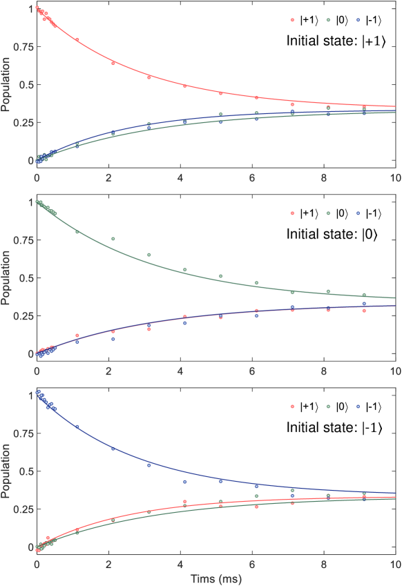
Figure S10: Three-level longitudinal relaxation. The relaxation behaviors of the NV electron spin ($S=1$) are measured with different initial states marked in each graph. The red, green, and blue dots stand for the states $|+1\rangle$, $|0\rangle$, and $|-1\rangle$, respectively. The solid lines are plotted by simultaneously fitting the nine groups of data points above.

where $\rho_{+1}(t)$, $\rho_{0}(t)$, and $\rho_{-1}(t)$ correspond to the evolutions with initial states $m_{\scaleto{S}{4.5pt}}=+1$, $0$, and $-1$, respectively. Based on Eq. (Gate error analysis), nine experiments are performed with all three states prepared and readout after a waiting time, with the results shown in Fig. S10. By simultaneously fitting all data points with the nine functions from Eq. (Gate error analysis), the decay matrix is determined to be

$$\Gamma=\begin{pmatrix}-229(6)&98(4)&130(5)\\ 98(4)&-198(6)&100(4)\\ 130(5)&100(4)&-230(6)\\ \end{pmatrix}$$ (S25)

where the unit of each value in the matrix is s^-1, and all values in parentheses stand for one standard deviation. With the equation $((\gamma_{+1}+\gamma_{2})/2+\gamma_{-1})T_{\text{CNOT}}$, the error from the longitudinal relaxation is estimated to be 0.32‰.

Compared with the primitive gate, the gate realized by the shaped pulse in realistic settings, inevitably suffers more from the problem of waveform distortion, owing to the complicated profile optimized for the effect of DEC. Unlike the errors from various fluctuations, the waveform distortion gives rise to a deterministic error, namely, a unitary error. Thus, the error from the waveform distortion can be estimated by constructing the density matrix after implementing each RB and IRB sequence. The population of the state after each sequence has been provided by the RB and IRB results, while the real part and the imaginary part of the coherence are measured by applying a $\pi_{y}/2$ pulse and a $\pi_{x}/2$ pulse respectively before reading out the state, with the results shown in Fig. S11-S12. With the density matrix, the quantum-state purity is calculated for the state after implementing each sequence, and represents an estimated fidelity without the waveform distortion. The fidelity difference with and without the waveform distortion is the error arising therefrom. The error on the CNOT gate from the waveform distortion is estimated to be 0.21‰ from the IRB results after subtracting that on single-qubit Cliffords from the RB results.

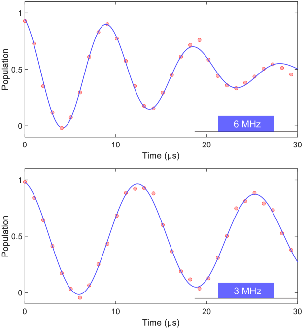
Figure S13: Measured instability of microwave amplitude. Undersampling measurements of the Rabi oscillations with two amplitudes (6 MHz and 3 MHz) are used for evaluating the instability of the microwave amplitude. The data in each graph are accumulated by running the experiment for about 5 hours, and the solid lines are the fitting curves with the function $a\cos(2\pi(\delta f)t+\phi_{0})e^{-(t/T_{2}^{\prime})^{2}}+b$.

Gate errors from other sources are small enough. First, we analyze the error from the instability of the MW amplitude. As shown in Fig. S13, Rabi oscillations with long durations are measured in an undersampling manner for the amplitudes 6 MHz and 3 MHz. The decay behavior is close to $e^{-(t/T_{2}^{\prime})^{2}}$, different from that in the work [10]. Therefore, the normalized amplitude with respect to the absolute value (6 MHz and 3 MHz), is supposed to comply with a Gaussian distribution, and the instabilities are fitted to be 0.018(2) for 6 MHz and 0.015(2) for 3 MHz. Here we use the value of 0.018 in the simulation to take up an estimated error of 0.030‰. Second, the gate error is caused by the approximations used for deriving the system Hamiltonian (S8), including the rotation wave approximation (RWA) and the reduction into the four-level structure. The latter gives rise to the population leakage into the third level $m_{\scaleto{S}{4.5pt}}=+1$. The arising error is given by 0.020‰  by calculating the gate realized by the shaped pulse under the natural Hamiltonian (S2). Third, the ¹⁴N-nuclear-spin decoherence, mainly caused by the applied pulse not by the ¹³C spin bath, will disturb the superposition between two nuclear subspaces. The error from the nuclear decoherence is estimated to be $7\times 10^{-6}$, which justifies the assumption for the method of SRB. The errors from other sources are all below $10^{-6}$, including the inaccuracy of the coupling parameter used for the optimization of the shaped pulse (2159.88 kHz), the nuclear decoherence from the ¹³C spin bath, the sideband effect from the $z$ component of the MW pulse, the manipulation of the MW pulse on the ¹⁴N nuclear spin, and so on.

\begin{overpic}[width=433.62pt]{C13.pdf} \put(13.0,57.0){{\large}{(a)}} \put(0.0,46.0){{\large}{(b)}} \put(50.0,46.0){{\large}{(c)}} \put(0.0,24.0){{\large}{(d)}} \put(50.0,24.0){{\large}{(e)}} \end{overpic}

Figure S2: Detection of the strongly coupled ¹³C spins with the NV spin coherence under DD sequences. (a) The DD sequence with 32 $\pi$ pulses (DD-32). The interval between two $\pi$ pulses is denoted by $\tau$. (b-e) Measured coherence under the DD-32 sequence with different orders $k$ for acquiring the coupling parameters of the five ¹³C spins in the table of Fig. 1(c). The horizontal axis is the interval $\tau$ between two $\pi$ pulses in (a). The coupling parameters of the first ¹³C spin are obtained by fitting two dips ($k=$ 4 and 5) in (b) with Eq. (S10). The solid line is the fitting curve plotted for comparison. The same procedures are performed for the other four ¹³C spins with the results of (c-e).

\begin{overpic}[width=433.62pt]{Classical_noise.pdf} \put(0.5,67.3){{\large}{(a)}} \put(51.0,67.3){{\large}{(b)}} \put(25.5,32.5){{\large}{(c)}} \end{overpic}

Figure S3: Measurement of the weakly coupled ¹³C spins taken as classic noise. (a) The NV spin coherence measured under a Ramesy sequence. The green line is data fitting using the function $a\cos(2\pi(\delta f)t+\phi_{0})e^{-(t/T_{2}^{*})^{p}}+b$ with $\delta f$ denoting the detuning. The blue line is plotted based on a numerical simulation, where the nearby five ¹³C spins and the static noise from the weakly coupled ¹³C spins (obtained in (b)) are considered. (b) The resultant decoherence from the weakly coupled ¹³C spins by deducting the contribution of the nearby five ¹³C spins from (a). The strength of the static noise from the weakly coupled ¹³C spins is obtained to be $\sigma=$ 20.0(1.5) kHz by fitting the results with the function $e^{-(2\pi\sigma t)^{2}/2}$. (c) The resonance dip of the weakly coupled ¹³C spins under the 32-DD sequence, obtained from the dip indicated by the label “¹³C Bath” in Fig. 1(b) of the main text after subtracting the contribution of the nearby five ¹³C spins. The dashed line is the numerical simulation under the time-varying noise with the strengths $\sigma_{x}=\sigma_{y}=$ 30 kHz.

\begin{overpic}[width=433.62pt]{Heat.pdf} \put(0.0,61.0){{\large}{(a)}} \put(0.0,32.0){{\large}{(b)}} \end{overpic}

Figure S9: Measurement of the heating effect. (a) The heating effect measured with the sequence in (b) for the single-qubit RB (left) and the IRB for the CNOT gate (right), both of which are invisible within the errorbars. (b) The sequence for measuring the heating effect mainly induced by the RB sequence and the RF pulses. Compared with Fig. S8, the RB sequence is off-resonant by 1 GHz with its duration added into the idle stage of the reference sequence.

\begin{overpic}[width=208.13574pt]{Tomo_SQ_0.pdf} \end{overpic}

\begin{overpic}[width=208.13574pt]{Tomo_SQ_1.pdf} \end{overpic}

Figure S11: State tomography after single-qubit RB. The state tomography after the 100-Clifford RB sequences in both $m_{\scaleto{I}{4.5pt}}=+1$ (left) and $m_{\scaleto{I}{4.5pt}}=0$ (right) subspaces is performed for evaluating the error from the waveform distortion of the shaped pulse. The results of the $\pi_{x}/2$ gate (upper) an the $\pi_{y}/2$ gate (lower) together with the corresponding RB result (no gate) constitute a full single-qubit tomography.

\begin{overpic}[width=208.13574pt]{Tomo_CNOT_0.pdf} \end{overpic}

\begin{overpic}[width=208.13574pt]{Tomo_CNOT_1.pdf} \end{overpic}

Figure S12: State tomography after CNOT-gate IRB. The state tomography after the IRB sequences with 50 CNOT gates included is performed in both $m_{\scaleto{I}{4.5pt}}=+1$ (left) and $m_{\scaleto{I}{4.5pt}}=0$ (right) subspaces for evaluating the error from the waveform distortion of the shaped pulse. The results of the $\pi_{x}/2$ gate (upper) an the $\pi_{y}/2$ gate (lower) together with the corresponding IRB result (no gate) constitute a full single-qubit tomography.

References

• Xie et al. [2021] T. Xie, Z. Zhao, M. Guo, M. Wang, F. Shi, and J. Du, Identity test of single NV- centers in diamond at Hz-precision level, Phys. Rev. Lett. 127, 053601 (2021).
• Taminiau et al. [2012] T. H. Taminiau, J. J. T. Wagenaar, T. Van der Sar, F. Jelezko, V. V. Dobrovitski, and R. Hanson, Detection and control of individual nuclear spins using a weakly coupled electron spin, Phys. Rev. Lett. 109, 137602 (2012).
• Biercuk et al. [2009] M. J. Biercuk, H. Uys, A. P. VanDevender, N. Shiga, W. M. Itano, and J. J. Bollinger, Optimized dynamical decoupling in a model quantum memory, Nature 458, 996 (2009).
• Ma et al. [2015] W. Ma, F. Shi, K. Xu, P. Wang, X. Xu, X. Rong, C. Ju, C.-K. Duan, N. Zhao, and J. Du, Resolving remote nuclear spins in a noisy bath by dynamical decoupling design, Phys. Rev. A 92, 033418 (2015).
• Khaneja et al. [2005] N. Khaneja, T. Reiss, C. Kehlet, T. Schulte-Herbrüggen, and S. J. Glaser, Optimal control of coupled spin dynamics: design of NMR pulse sequences by gradient ascent algorithms, J. Magn. Reson. 172, 296 (2005).
• Baldwin et al. [2020] C. H. Baldwin, B. J. Bjork, J. P. Gaebler, D. Hayes, and D. Stack, Subspace benchmarking high-fidelity entangling operations with trapped ions, Phys. Rev. Res. 2, 013317 (2020).
• Magesan et al. [2012] E. Magesan, J. M. Gambetta, B. R. Johnson, C. A. Ryan, J. M. Chow, S. T. Merkel, M. P. Da Silva, G. A. Keefe, M. B. Rothwell, T. A. Ohki, et al., Efficient measurement of quantum gate error by interleaved randomized benchmarking, Phys. Rev. Lett. 109, 080505 (2012).
• Magesan et al. [2011] E. Magesan, J. M. Gambetta, and J. Emerson, Scalable and robust randomized benchmarking of quantum processes, Phys. Rev. Lett. 106, 180504 (2011).
• Pedersen et al. [2007] L. H. Pedersen, N. M. Møller, and K. Mølmer, Fidelity of quantum operations, Phys. Lett. A 367, 47 (2007).
• Rong et al. [2015] X. Rong, J. Geng, F. Shi, Y. Liu, K. Xu, W. Ma, F. Kong, Z. Jiang, Y. Wu, and J. Du, Experimental fault-tolerant universal quantum gates with solid-state spins under ambient conditions, Nat. Commun. 6, 8748 (2015).
Refer to caption