Searches for Mass-Asymmetric Compact Binary Coalescence Events using Neural Networks in the LIGO/Virgo Third Observation Period

Abstract

We present the results on the search for the coalescence of compact binary mergers with very asymmetric mass configurations using convolutional neural networks and the LIGO/Virgo data for the O3 observation period. Two-dimensional images in time and frequency are used as input. Masses in the range between 0.01 $\rm{M\textsubscript{$\odot$}}$ and 20 $\rm{M\textsubscript{$\odot$}}$ are considered. We explore neural networks trained with input information from a single interferometer, pairs of interferometers, or all three interferometers together, indicating that the use of the maximum information available leads to an improved performance. A scan over the O3 data set using the convolutional neural networks for detection results into no significant excess from an only-noise hypothesis. The results are translated into 90$\%$ confidence level upper limits on the merger rate as a function of the mass parameters of the binary system.

I Introduction

Since the discovery of Gravitational Waves (GW) in 2015 Abbott et al. (2016a), generated by a compact binary coalescence (CBC) of black holes (BH), the LIGO and Virgo experiments have improved their sensitivity and observed an increasing number of GW signals, including also events attributed to the coalescence of neutron stars (NS), as well as the coalescence of BH-NS binary systems. The latest catalogue of events, from O1, O2 and O3 observation runs, collects a total of 90 events, dominated by BH-BH candidates Abbott et al. (2019a, 2020a); Abbott et al. (2021). The data indicate that the masses in the binary systems range between $1.17$ M_$\odot$(GW191219_163120) and $105$ M_$\odot$(GW190426_190642), with a mass ratio $q\equiv m_{1}/m_{2}$, where $m_{1}$ denotes the heaviest of the two objects, in the range between $1.1$ (GW170817) and $26.5$ (GW191219_163120). The LIGO and Virgo Collaborations use matched-filtering techniques to extract the events from the much larger background (for a comprehensive review of the experimental techniques see Ref. Abbott et al. (2020b)). The use of machine learning tools has been extensively explored in LIGO and Virgo (for a comprehensive review see Ref. Cuoco et al. (2020)). In particular, the presence of a distinct chirp-like shape in the CBC events, when represented in spectrograms showing the signal in frequency-time domain, makes the use of a convolutional neural network (CNN) a valid alternative suitable for GW detection Gabbard et al. (2018); George and Huerta (2017); Gebhard et al. (2019); George and Huerta (2018); Menéndez-Vázquez et al. (2021). In addition, the use of CNNs has been explored to distinguish between families of glitches Razzano and Cuoco (2018); Biswas et al. (2013); Cavaglia et al. (2019).

In this paper, we explore the implementation of a CNN for the identification of CBC events with very asymmetric mass configurations with $q<2000$, and $m_{1}$ and $m_{2}$ in range between $1$ – $20$ M_$\odot$ and $0.01$ – $1$ M_$\odot$, respectively. This is motivated by the search for CBC candidates with the presence of subsolar-mass (SSM) BHs. Since there is no well-established astrophysical explanation for the origin of SSM BHs, their discovery would point to the presence of new physics. The presence of SSM BHs are predicted by different models, including primordial black holes (PBHs) from the the collapse of overdensities in the early universe Hawking (1971); Carr and Hawking (1974); Hütsi et al. (2019, 2021); gravitational collapse of dark matter halos D’Amico et al. (2018); Khlopov (2010); Belotsky et al. (2014); Shandera et al. (2018); the accumulation of dark matter by neutron stars leading to SSM BHs Kouvaris and Tinyakov (2011); or SSM boson stars Kaup (1968); Guo et al. (2019); Colpi et al. (1986). As illustrated in Figure 1, this study complements the phase space in mass considered by previous searches for SSM events using O3 data and matched-filtering based selections Abbott et al. (2021); Abbott et al. (2022a); Nitz and Wang (2022); Abbott et al. (2022b). Previous results using other observational periods are included in Refs. Nitz and Wang (2021a); Nitz et al. (2021); Phukon et al. (2021); Abbott et al. (2019b).

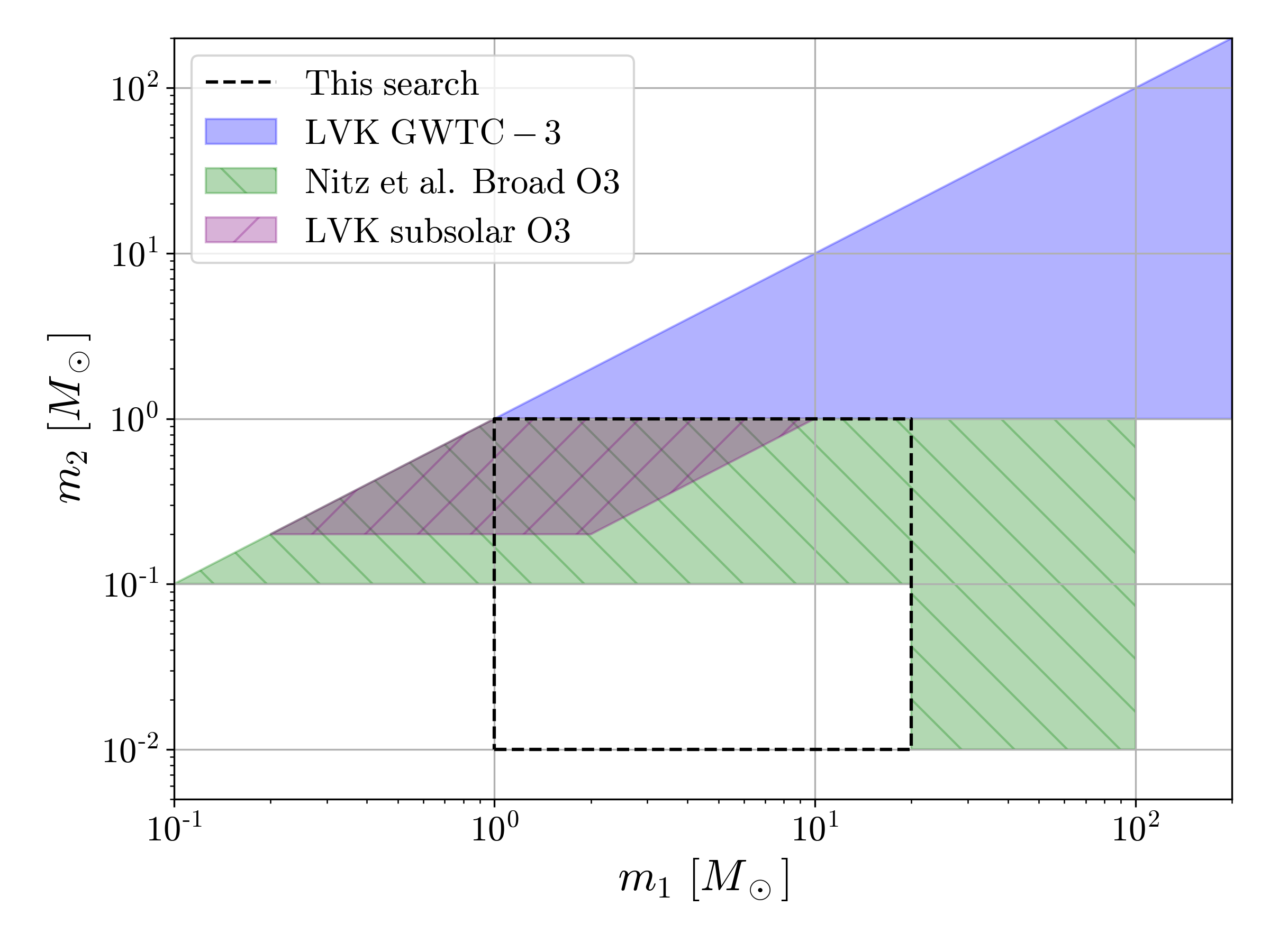
Figure 1: Region of interest compared to other recent searches. The blue region is the one searched by the LVK collaboration as part of the GWTC-3 catalog Abbott et al. (2021), the magenta hatched region corresponds to the LVK subsolar mass targeted search performed over O3 data Abbott et al. (2022a); Abbott et al. (2022b) while the green hatched region corresponds to the broad search performed by Nitz and Wang over the O3 data Nitz and Wang (2022).

II Data Preparation

The study uses the O3 data from LIGO-Hanford (H1), LIGO-Livingston (L1) and Virgo (V1) interferometers with 4096 Hz sampling rate. After imposing quality requirements, dealing with the understanding of the interferometer stationary noise budget as well as the identification and suppression of glitches and spectral noise contributions (for a comprehensive discussion see Refs. The LIGO Scientific Collaboration (2021); Virgo Collaboration (2022)), the H1-L1-V1 combined samples have a total duration of 155 days. The H1-L1-V1 O3 data is used for constructing an image containing a spectrogram with only background and background plus injected signal for the purposes of the CNN training. Special precaution was taken in the preparation of the background images to exclude any of the identified GWs events in O3, as collected in the GWTC-3 catalog Abbott et al. (2021). A total of $142,944$ images were used. The results obtained (see below) show that this number of images is enough for an adequate training and validation of the network. The images are divided as follows: $115,200$ $(80.6\%)$ for training, $12,800$ $(9.0\%)$ for validating and $14,944$ ($10.4\%$) for testing, evenly distributed into background-only and background with a signal injected.

Waveforms for GW signals are generated using PyCBC Usman et al. (2016); Nitz et al. (2017, 2020) with the IMRPhenomD Husa et al. (2016); Khan et al. (2016) model and combined with data segments from the different interferometers, after taking into account the proper relative orientations, times of arrival and antenna factors. The parameters considered are uniformly sampled, as described in Table 1, and zero spin components are assumed. Masses in the range between 1 - 20 $\rm{M\textsubscript{$\odot$}}$ (0.01 - 1 $\rm{M\textsubscript{$\odot$}}$) are considered for $m_{1}$ ($m_{2}$), and the corresponding luminosity distance $D_{\rm{L}}$ is limited to nearby events in the range 1 - 100 Mpcs. Other parameters related to the position in the sky and orientation of the source are taken as homogeneously distributed.

$m_{1}~{}[\rm{M\textsubscript{$\odot$}}]$	$m_{2}~{}[\rm{M\textsubscript{$\odot$}}]$	$D_{\rm{L}}~{}[$Mpc$]$	$\psi$	$\theta_{JN}$	$\alpha$	$\cos(\delta)$
$[1,20]$	$[0.01,1]$	$[1,100]$	$\left[0,\pi/2\right]$	$[0,\pi]$	$[0,2\pi]$	$[-1,1]$

Table 1: Range of the uniformly sampled variables for the training set, being $(m_{1},m_{2})$ the component masses, $D_{\rm{L}}$ the luminosity distance, $\psi$ the inclination of the orbit with respect to the line of sight, $\theta_{JN}$ the polarization of the gravitational wave and $(\alpha,\delta)$ the right ascension and declination, respectively.

The injected signals are limited to a fixed maximum duration of five seconds. The five-seconds window is computed backward from the merger time to remove low-amplitude monochromatic-like parts of the waveform and avoid confusing the network during training. A low frequency threshold of 45 Hz is applied in order to control the duration of the injected signal. Finally, the signals are randomly placed within the five-seconds window. Once the GW signals are injected in the different H1, L1 and V1 background segments, the data is processed. First, the time series are whitened following the same prescription as in Refs. Abbott et al. (2020b); Abbott et al. (2020c). Two-dimensional arrays holding spectrogram data are then produced using $Q$-transforms Brown (1991); Brown and Puckette (1992); Schörkhuber and Klapuri (2010) in order to arrive to the desired images in terms of amplitude vs time vs frequency, with 400 bins in time and 100 bins in frequency. Figure 2 presents an example of spectograms corresponding to a binary BH event with $m_{1}=2.6\ \rm{M\textsubscript{$\odot$}}$ and $m_{2}=0.35\ \rm{M\textsubscript{$\odot$}}$ at a distance of $3.4$ Mpcs. In the case of H1 and L1, the characteristic chirp is clearly observed.

In order to account for the presence of glitches in the data, not completely suppressed by the whitening process and leading to instabilities in the CNN training Ioffe and Szegedy (2015), the contents in each image are renormalized in such a way that they have an average equal to zero and a variance equal to one, following the same prescription as in Ref. Menéndez-Vázquez et al. (2021).

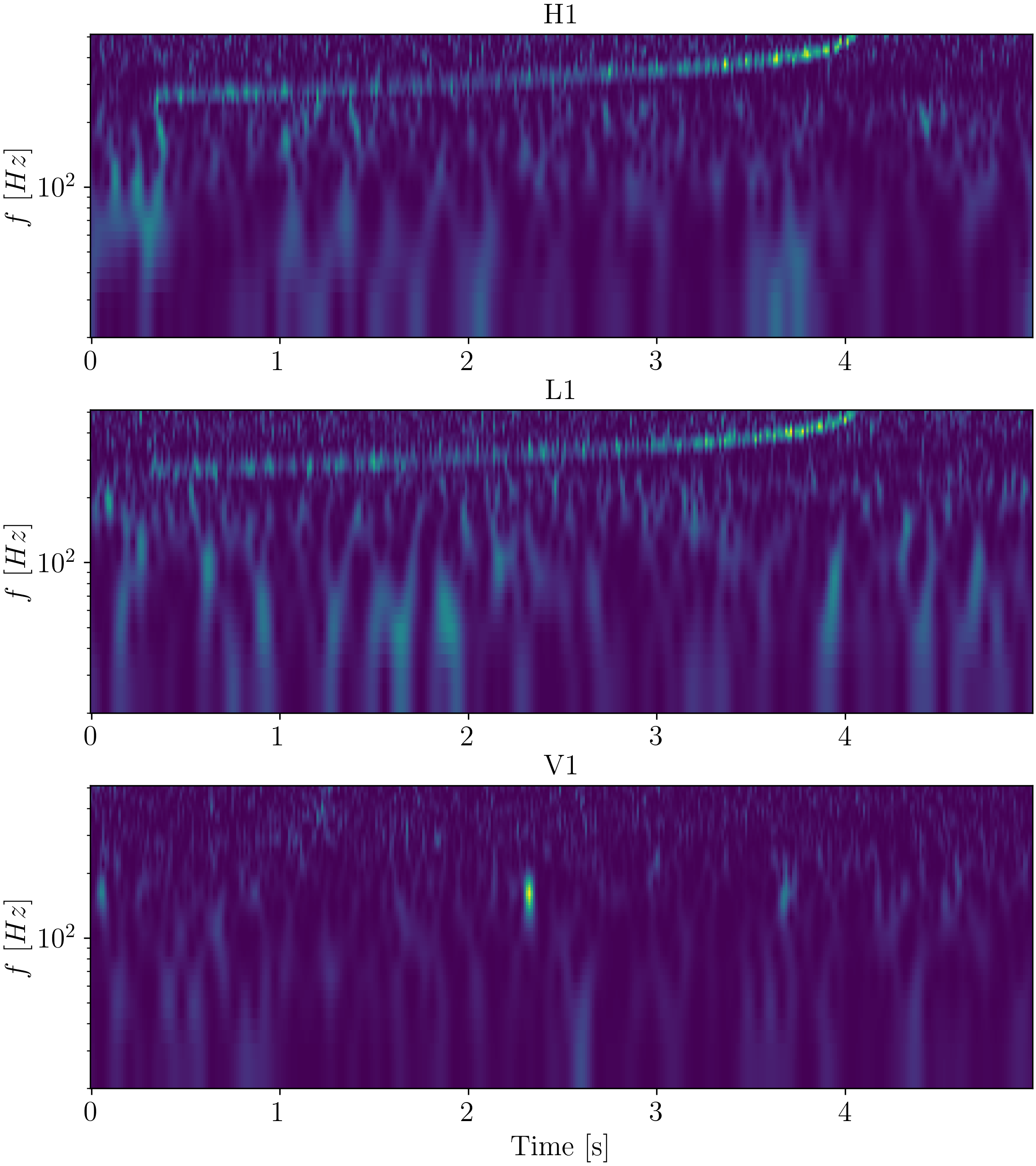
Figure 2: Spectrograms for a binary system with $m_{1}=2.6~{}\rm{M\textsubscript{$\odot$}}$ and $m_{2}=0.35~{}\rm{M\textsubscript{$\odot$}}$ and a distance $D_{\rm{L}}=3.4$ Mpcs, as seen in H1, L1 and V1.

III Neural network definition and training

This study closely follows that of Ref. Menéndez-Vázquez et al. (2021), using a ResNet50 architecture He et al. (2016a, b) (see Table 2) with modifications in the last layer, for which average pooling and a fully connected dense layer (1-d fc) with a sigmoid activation function are implemented. For the loss function, a binary cross-entropy is employed. Finally, a learning rate of $0.01$ alongside an Adam optimizer Kingma and Ba (2014); Ruder (2016); Goodfellow et al. (2016) and a batch size of $32$ are used for a total of $10$ epochs. With all these parameters, different CNNs have been trained using the GPU enhanced capabilities of Keras and TensorFlow Abadi et al. (2016).

We train seven different CNNs. Three CNNs are trained separately for H1, L1 and V1 data. In addition, three CNNs are trained for H1-L1, H1-V1, and L1-V1 pairs of input data, and one CNN is trained for H1-L1-V1 combined input data, where information from two or three interferometers are input simultaneously to the corresponding CNNs. As expected, the performances of the CNNs improve by including the information of multiple interferometers during the training process, since the CNN learns about correlations across images in different channels when the signal is present. Therefore, CNNs using single interferometer information are discarded for the final scan over the O3 data.

Layer name	Output size	Layer structure
conv1	112$\times$112	7$\times$7, 64, stride 2
conv2_x	56$\times$56	3$\times$3 max pool, stride 2
		$\left[\begin{array}[]{c}\text{1$\times$1, 64}\\[-0.80005pt] \text{3$\times$3, 64}\\[-0.80005pt] \text{1$\times$1, 256}\end{array}\right]$$\times$3
conv3_x	28$\times$28	$\left[\begin{array}[]{c}\text{1$\times$1, 128}\\[-0.80005pt] \text{3$\times$3, 128}\\[-0.80005pt] \text{1$\times$1, 512}\end{array}\right]$$\times$4
conv4_x	14$\times$14	$\left[\begin{array}[]{c}\text{1$\times$1, 256}\\[-0.80005pt] \text{3$\times$3, 256}\\[-0.80005pt] \text{1$\times$1, 1024}\end{array}\right]$$\times$6
conv5_x	7$\times$7	$\left[\begin{array}[]{c}\text{1$\times$1, 512}\\[-0.80005pt] \text{3$\times$3, 512}\\[-0.80005pt] \text{1$\times$1, 2048}\end{array}\right]$$\times$3
	1$\times$1	Global average pool, 1-d fc, sigmoid
Hyper parameters
Learning rate		0.01
Batch size		32
Number of epochs		10
Optimizer		Adam
Loss function		Binary-cross entropy

Table 2: CNN architecture and the associated hyper parameters. Building blocks are shown in brackets, with the numbers of blocks stacked. Downsampling is performed by conv3_1, conv4_1, and conv5_1 with a stride of 2 (partially taken from He et al. (2016a)).

Figure 3 shows, for the H1-L1-V1 case, the evolution of the accuracy and loss as a function of epochs, demonstrating stability after about eight to ten epochs, with an accuracy above 0.8 and a loss below 0.4. In addition, the validation accuracy is presented, demonstrating a healthy evolution of the training process. The final CNN output for the H1-L1-V1 case is shown in Figure 4, where a clear discrimination is obtained between signal and background samples. Similar features in the training process and the distribution of the final CNN discriminant are observed in the rest of CNNs.

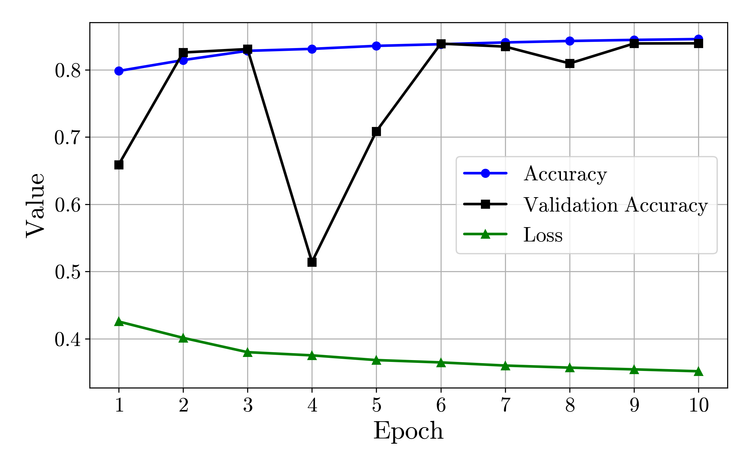
Figure 3: Accuracy, loss and validation accuracy during the training epochs for the H1-L1-V1 CNN.

The receiver operating characteristic (ROC) curves for the separate CNNs, representing the true positive (TP) versus the false positive (FP) rates are presented in Figure 5 for the H1-L1, H1-V1, L1-V1, and H1-L1-V1 CNNs. For very low FP rates, the TP rates only reach values around $70\%$, indicating a limited efficiency for event detection. The efficiency steadily increases at the cost of much larger FP rates. The ROC curve, along with a tolerable maximum false alarms rate (FAR) for detection, determines the final operating point of a given CNN. The computation of the FAR for each CNN follows the prescription in Ref. Abbott et al. (2016b). The FAR is defined as ${\rm{FAR(\eta)}}=N(\eta)/T$, where $\eta\in[0,1]$ is the CNN discriminant output, $N(\eta)$ is the number of events with a CNN discriminant above or equal to $\eta$ and $T$ the period of time analysed. In order to effectively increase the time considered in the calculation, reaching very low FAR values, the time slide technique Abbott et al. (2005); Abbott et al. (2016b) is used. This allows accumulating $\mathcal{O}(10^{9})$ images of $5$ s duration each and accessing FAR values down to $1/152.6$ years^-1.

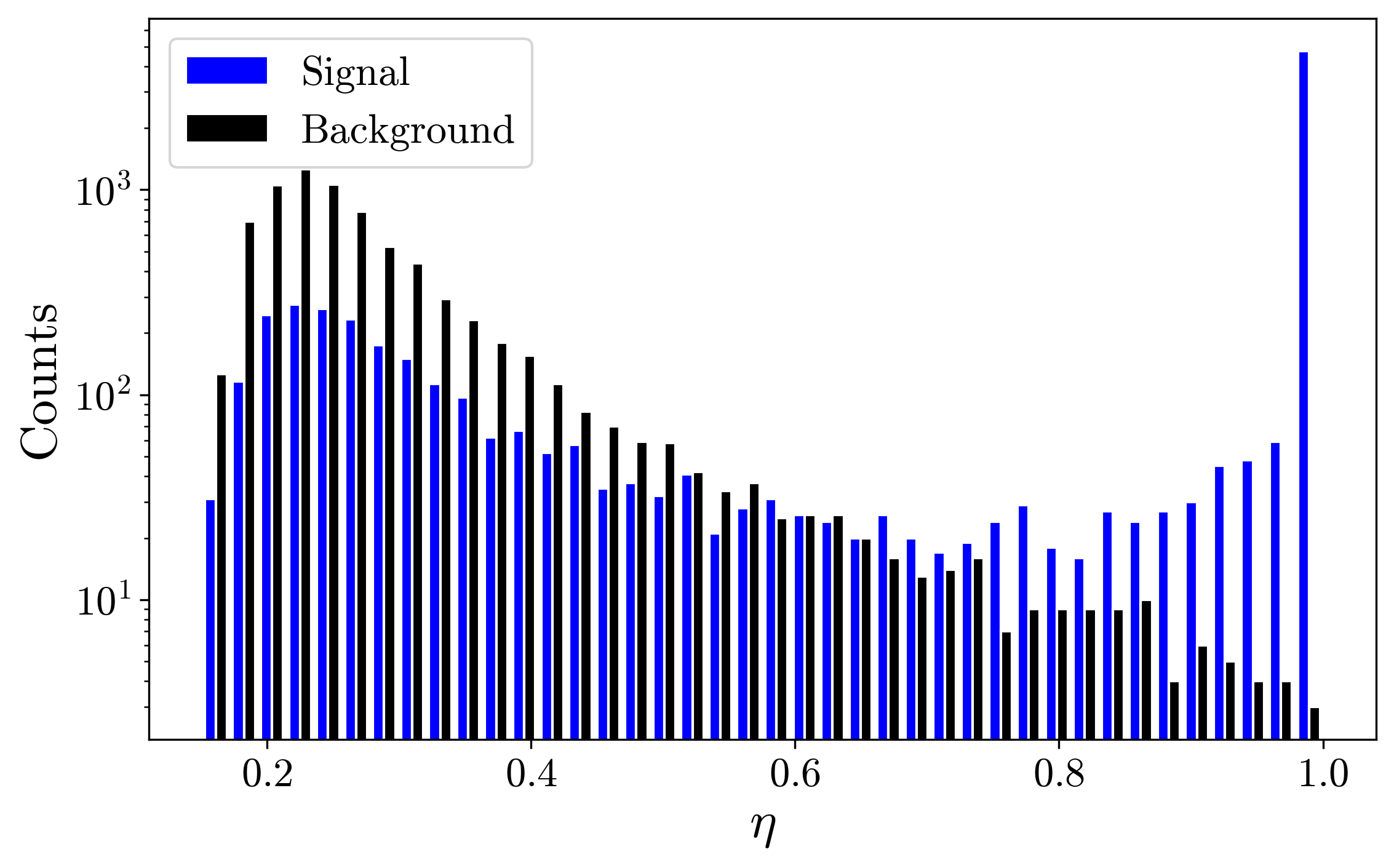
Figure 4: CNN discriminating output corresponding to the H1-L1-V1 case for background and signal images.

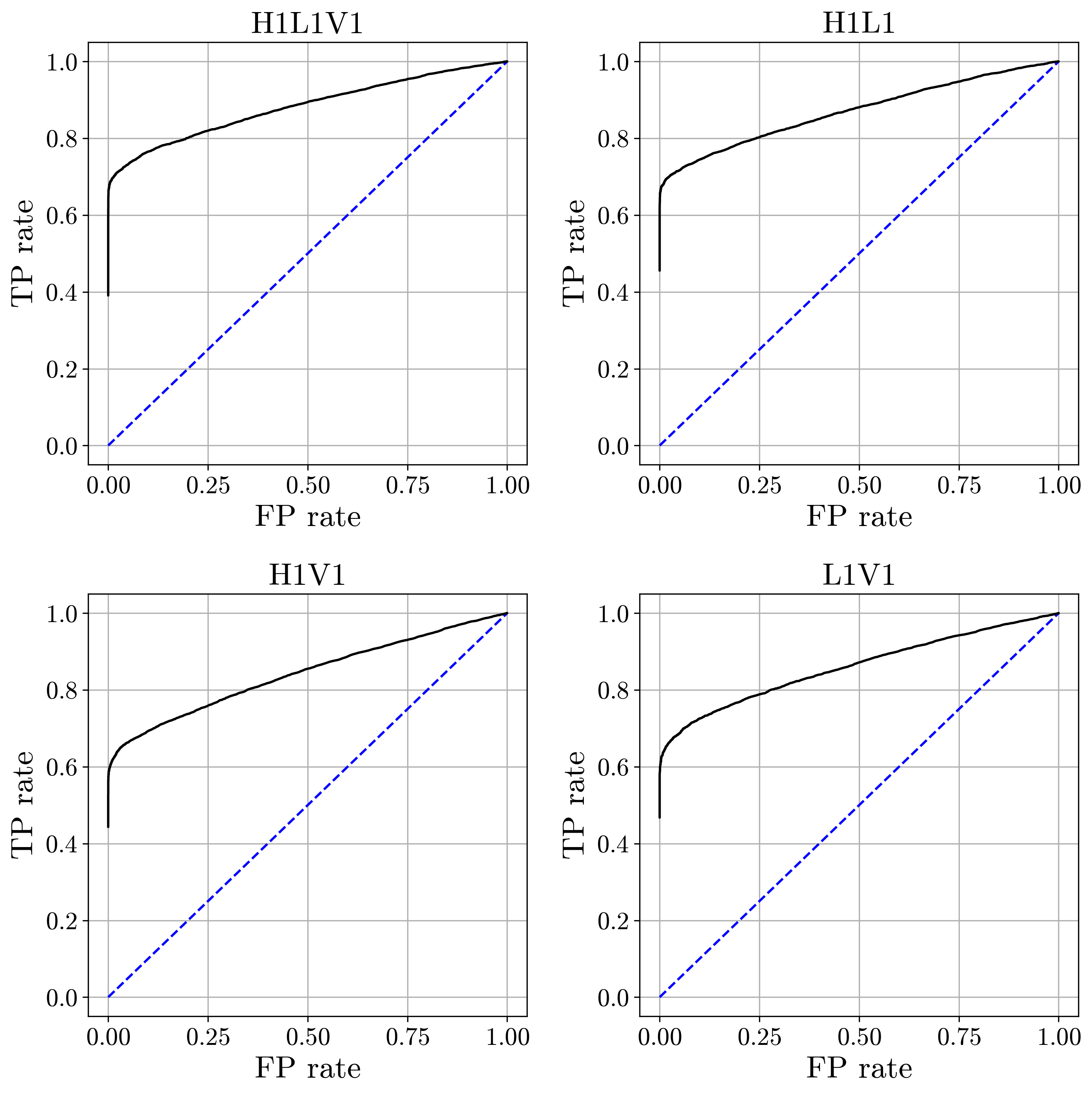
Figure 5: ROC curves for the different CNNs.

We initially establish a CNN discriminant $\eta_{0}$ corresponding to a $\rm{FAR(\eta_{0})}$ value of $1$ years^-1. However, the number of FP detected remains sizable when $\eta_{0}\to 1$ and the CNNs never reach a discriminant capable of producing only one false positive event per year. A further improvement of the global sensitivity is achieved by combining the outputs of the separate CNNs into a global discriminant. Such combination provides an additional tool for suppressing glitches in the data affecting independently the interferometers and in different time stamps. A simple average of the H1-L1-V1, H1-L1, L1-V1, and H1-V1 CNN outputs has been considered. Alternatively, a number of algorithms, potentially giving different weights to different CNNs, were explored leading to very similar or even worse results. The resulting discriminant is presented in Figure 6 demonstrating an improved separation between background and signal, leading to a higher significance for the events finally selected as signal. Table 3 collects the corresponding detection rates and the computed FAR upper limit in the case of $\eta_{0}=1$ for the separate CNNs and their combination, where only the latter shows FAR values less than 1 event per year.

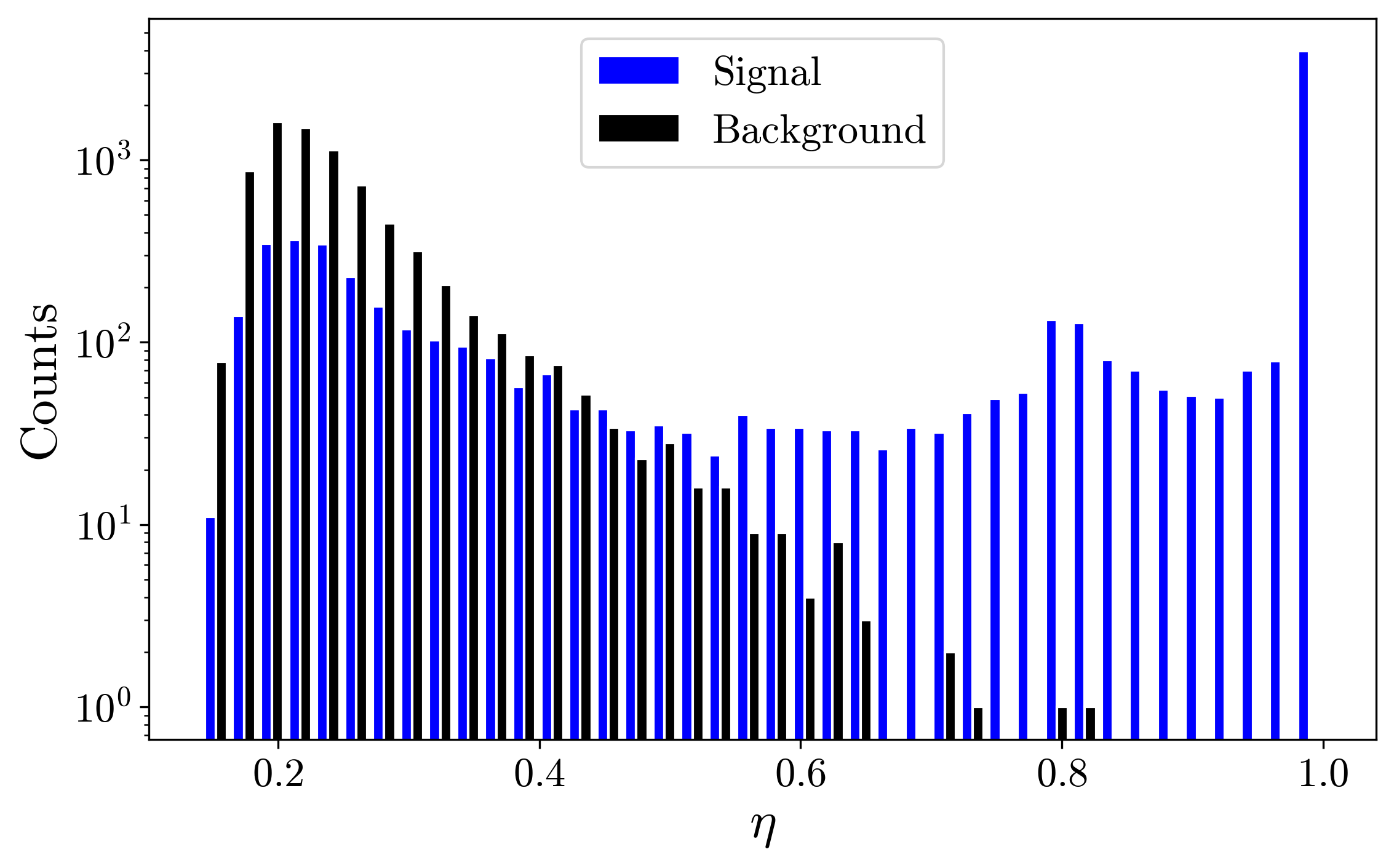
Figure 6: CNN global discriminating output corresponding to the average of the H1-L1-V1, H1-L1, L1-V1, and H1-V1 CNN outputs for background and signal images.

CNN	Threshold	TP rate	FP rate	$\rm{FAR(\eta_{0}=1)}$ $[$yrs${}^{-1}]$
H1 – L1	$1.0$	$0.46$	$\leq 2\cdot 10^{-4}$	$\sim 10^{2}$
L1 – V1	$1.0$	$0.47$	$\leq 2\cdot 10^{-4}$	$\sim 10^{3}$
H1 – V1	$1.0$	$0.44$	$\leq 2\cdot 10^{-4}$	$\sim 10^{2}$
H1 – L1 – V1	$1.0$	$0.58$	$\leq 2\cdot 10^{-4}$	$\sim 10^{3}$
Combined	$0.998$	$0.50$	$\leq 2\cdot 10^{-4}$	$\sim 10^{-2}$

Table 3: Anticipated TP and FP rates and FAR for the different CNNs and a discriminant $\eta_{0}=1$. The FP rates represent a 95% confidence level upper limits according to a null observation of FP in the testing set assuming Poisson statistics.

Signal injection studies are performed to establish the sensitivity of the different CNNs to the presence of a GW signal. For each GW signal, the signal-to-noise ratio (SNR), $\rho$, is computed following the prescription in Ref. Gabbard et al. (2018) solving the integral

$$\rho^{2}=4\ \int_{f_{\rm{min}}}^{f_{\rm{max}}}{\rm d}f\ \frac{|\tilde{h}(f)|^{2}}{S_{n}(f)},$$ (1)

in the frequency domain $(f)$, where $\tilde{h}(f)$ denotes the signal in the frequency domain and $S_{n}(f)$ the power spectral density of the background. A Tukey window with $\alpha=1/9$ is considered for the Fourier transform. The SNR defined above refers to each of the interferometers separately. Following the work in Refs. Littenberg et al. (2016); Lee et al. (2021), when appropriate we define a network SNR, $\rho_{\rm net}$, as

$$\rho_{\rm net}^{2}=\sum_{i}\rho_{i}^{2}\ ,$$ (2)

where $i$ denotes the different interferometers. Figure 7 shows the fraction of GW signals identified by the CNNs as a function of $\rho_{\rm net}$ in the different cases. As expected, the efficiency for signal detection increases rapidly with increasing SNR, becoming more efficient for large $\rho_{\rm net}$ values and improving with the inclusion of information from multiple interferometers. The best results are obtained by the H1-L1-V1 CNN. The results from the combination of CNNs is a compromise between the H1-L1-V1 CNN and the rest. Events with $\rho_{\rm net}\geq 25$ would be detected with an efficiency above 95$\%$ in the case of the H1-L1-V1 CNN. Table 4 collects the values of $\rho_{\rm net}$ at given detection efficiencies for the different CNNs.

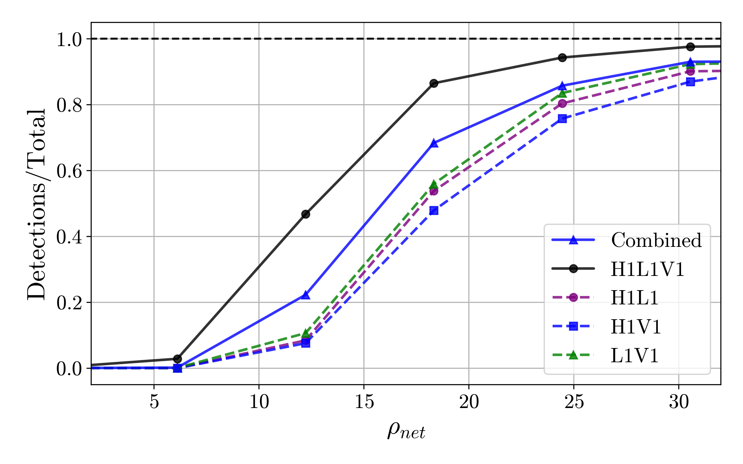
Figure 7: Signal detection efficiency as a function of $\rho_{\rm net}$ for the different CNNs and their combination.

CNN	$\rho_{\rm net}(80\%)$	$\rho_{\rm net}(90\%)$	$\rho_{\rm net}(95\%)$
H1 – L1	$24.4$	$30.5$	$42.0$
L1 – V1	$23.7$	$29.0$	$41.2$
H1 – V1	$26.8$	$21.1$	$25.8$
H1 – L1 – V1	$17.3$	$21.1$	$25.8$
Combined	$22.4$	$28.0$	$40.1$

Table 4: Values of $\rho_{\rm net}$ at given detection efficiencies for the different CNNs and the combination of outputs.

IV Results

We performed a scan of the full O3 data set, using the H1-L1-V1 combined sample, for which a slicing window of five seconds duration was used in steps of 2.5 seconds (leading to a 50$\%$ overlap between consecutive images) in each of the interferometers. This translates into more than eighty million images to be tested for the presence of potential signals. The CNN global discriminating output, defined as the average of the H1-L1-V1, H1-L1, L1-V1, and H1-V1 CNN outputs, is used to search for signal of SSM events. A scan over the data using different global discriminating values in the range between 0 and 1 is performed. In each case, the corresponding FAR is computed. The computation time for the entire O3 scan has been of the order of $2,000$ CPU-hours (on an Intel${}^{\text{\textregistered}}$ Xeon${}^{\text{\textregistered}}$ CPU E5-2680 v4 @ 2.40GHz). This represents a major improvement compared with the typically required CPU-time for known matched filtering pipelines.

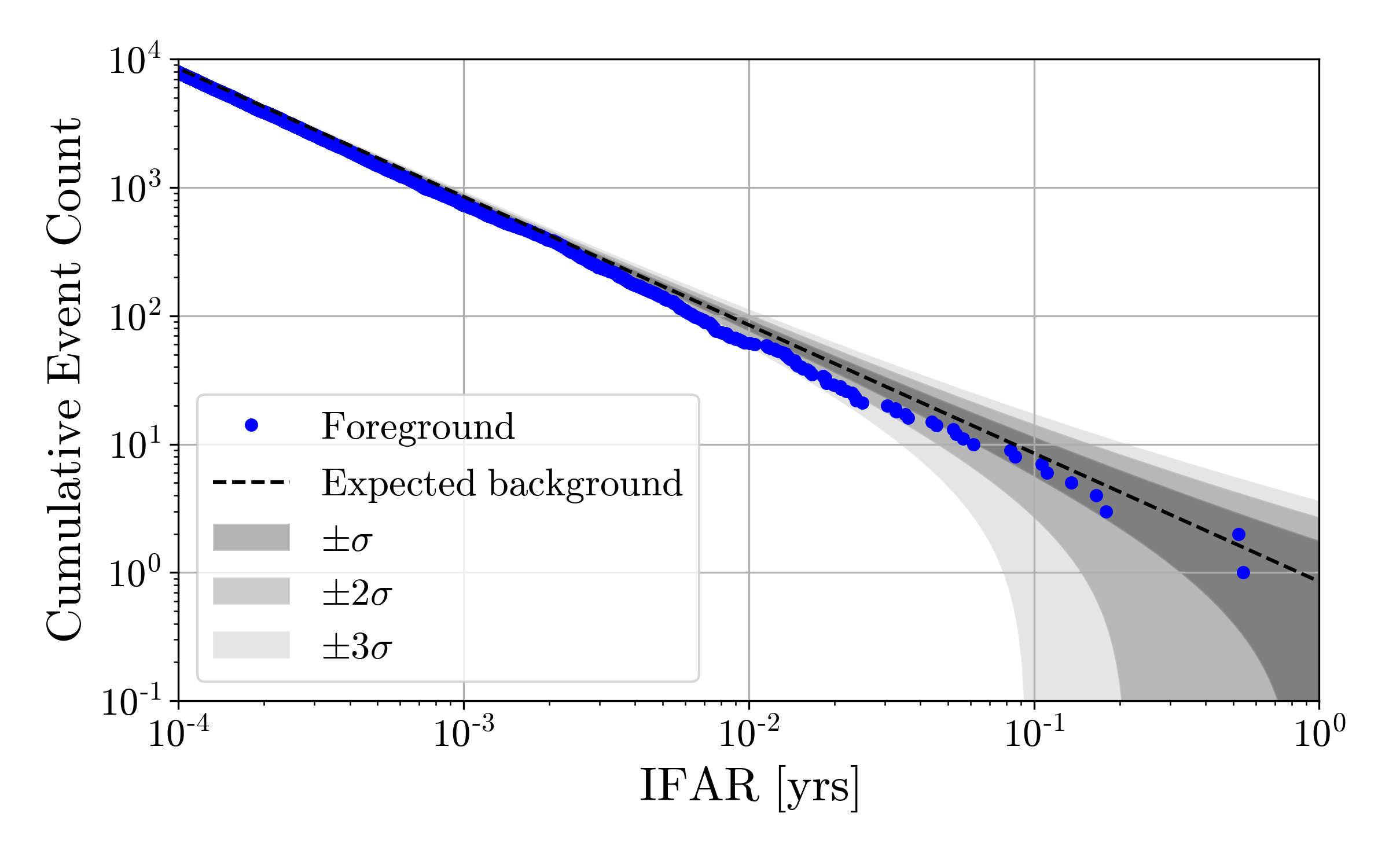
Figure 8: Observed cumulative event count as a function of the inverse false alarm rate for the O3 scan (dots). The data is compared to foreground predictions (dashed line) and including 1$\sigma$, 2$\sigma$, and 3$\sigma$ bands (shadowed areas).

The resulting inverse FAR distribution (IFAR), in units of years, is presented in Figure 8 compared to the expected yield of noise events following a Poisson probability distribution. No significant deviation from the expected noise is observed and no claim of SSM event detection can be made. For illustration purposes, Figure 9 shows the H1, L1 and V1 spectrograms for the most significant event having a FAR of $1.9$ years^-1, a combined CNN value equal to 0.9635, and CNN values equal to 0.9848, 0.9172, 0.9774 and 0.9747 for the H1-L1-V1, H1-L1, L1-V1, and H1-V1 neural networks, respectively.

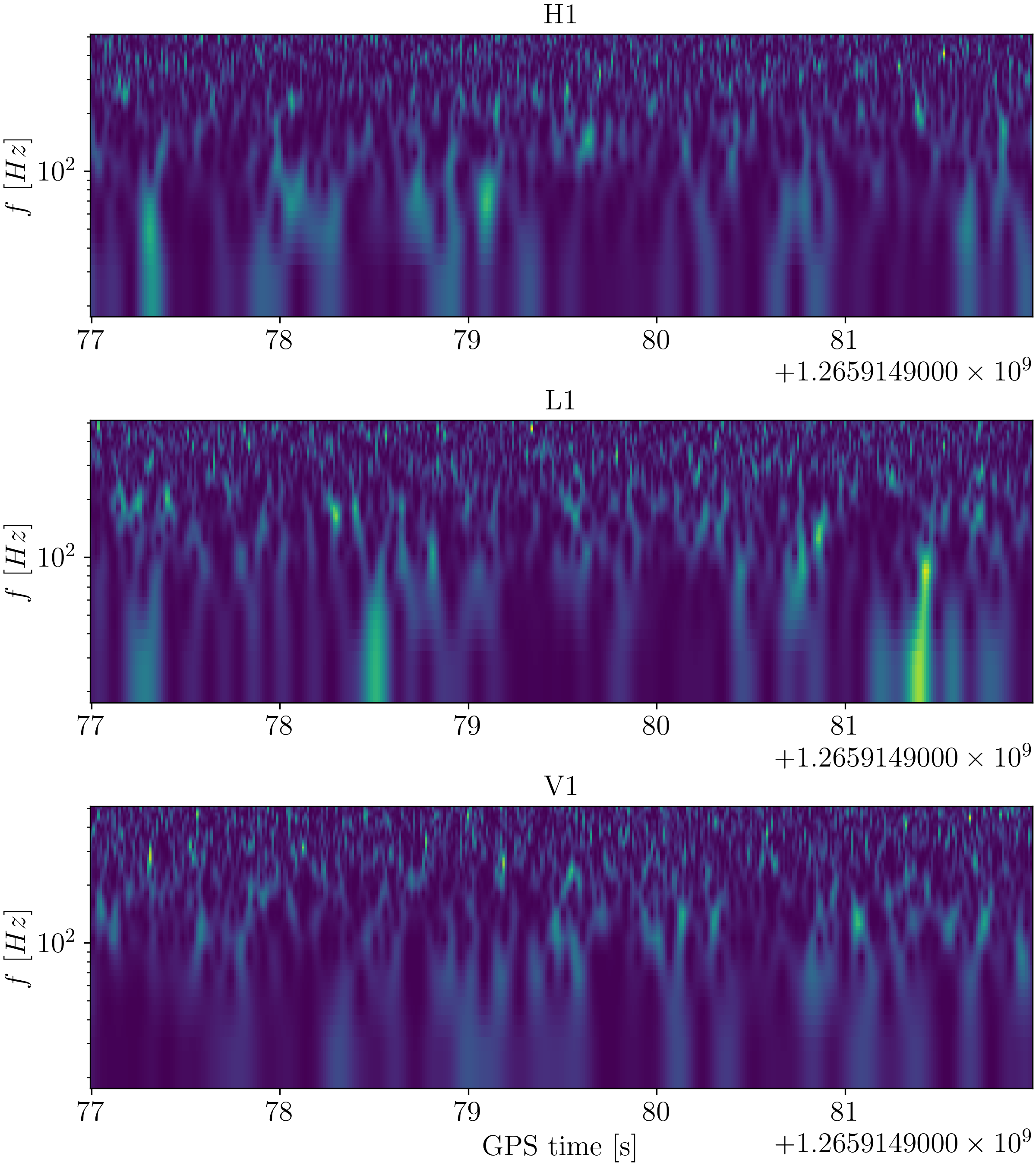
Figure 9: Spectrogram of the most significant image. Corresponds to a $\mathrm{FAR}=1.9~{}\mathrm{yrs}^{-1}$

The results are translated into 90$\%$ confidence level (CL) upper limits of the merger rate of binary systems in the range of masses and $q$ values considered. Since the sensitivity for detection mostly depends on the chirp mass of the binary system, defined as $\mathcal{M}_{c}\equiv\frac{(m_{1}m_{2})^{3/5}}{(m_{1}+m_{2})^{1/5}}$, the computed merger rates are binned in $\mathcal{M}_{c}$ instead of in the single masses of the binary system. The 90$\%$ CL upper limits are calculated using the loudest event statistics approach Tiwari (2018); Abbott et al. (2022a); Nitz and Wang (2021b, 2022); Abbott et al. (2022b) in terms of the surveyed time-volume $\langle VT\rangle$, following the expression

$$\mathcal{R}_{\rm{90}}=\frac{2.3}{\langle VT\rangle},\ \langle VT\rangle=T\ \int{\rm d}z\frac{1}{1+z}\frac{{\rm d}V_{c}}{{\rm d}z}\varepsilon(z),$$ (3)

where $T$ is the total observation time, $z$ denotes the redshift, $V_{c}$ is the comoving volume and $\varepsilon$ is the efficiency for detection. In this study $T$ is limited to $155$ days when H1, L1 and V1 interferometers were all taking data simultaneously. Figure 10 presents the detection efficiency of the combined CNN discriminant as a function of $z$ in several $\mathcal{M}_{c}$ bins. The efficiency is computed using injected signals and it vanishes for $z>0.06$. The integral above is marginalized over the rest of parameters of the binary system (see Table 1), which are considered homogeneously distributed in comoving volume.

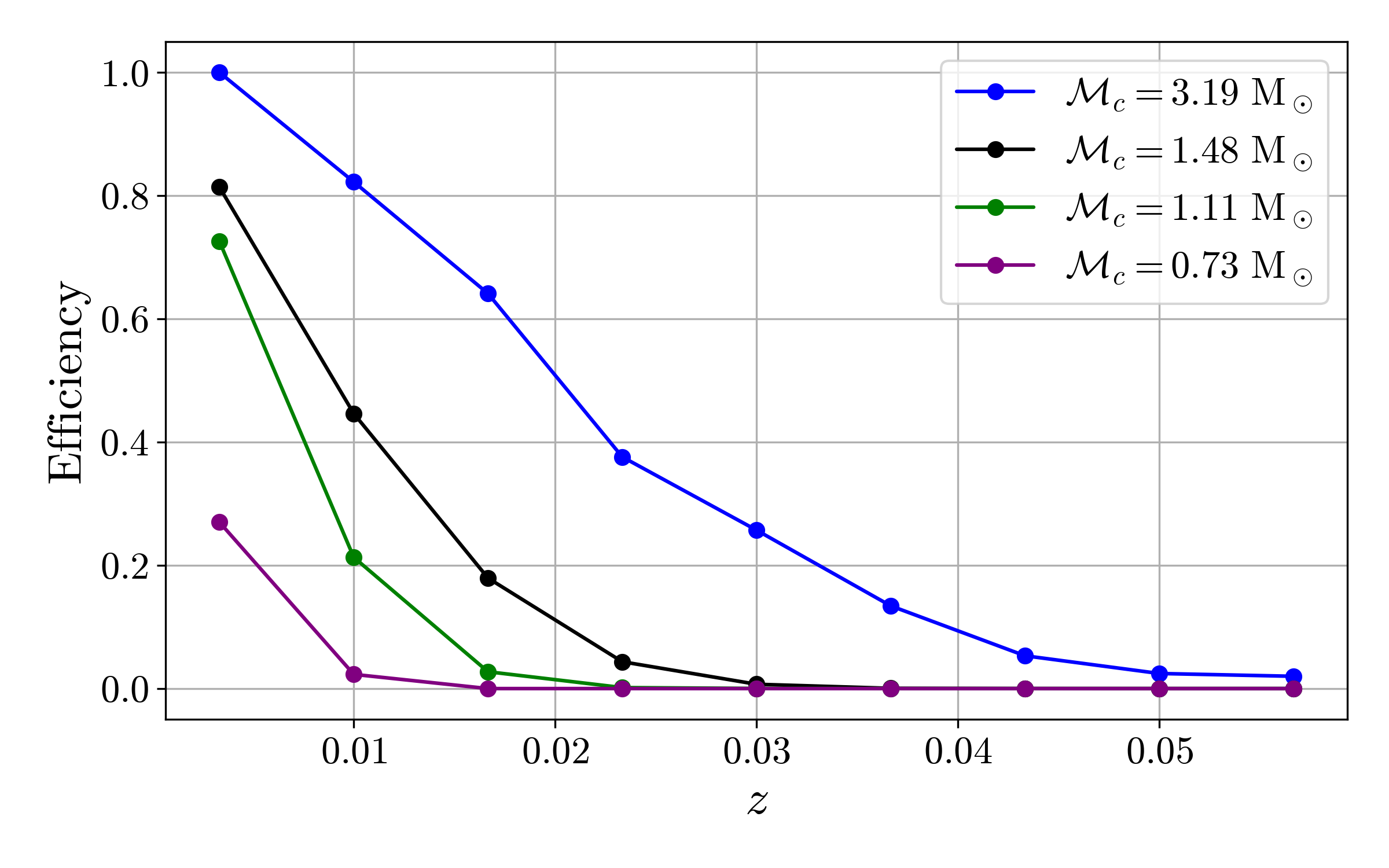
Figure 10: Detection efficiency for the combined CNN discriminant as a function of $z$ for different values of the chirp mass.

Figures 11 and  12 presents the 90$\%$ CL upper limits on the merging rate as a function of the chirp mass and as a function of $m_{2}$ in different $m_{1}$ regions, respectively. The results are compared to similar results from matched-filtering based analyses. Our result provides 90$\%$ CL upper limits in the range between $3\times 10^{6}~{}\mathrm{Gpc}^{-3}\mathrm{yrs}^{-1}$ and $560~{}\mathrm{Gpc}^{-3}\mathrm{yrs}^{-1}$ with increasing chirp mass, extending previous results to chirp masses up to 3 $\rm{M\textsubscript{$\odot$}}$. At lower chirp mass, our constrains are weaker than previous results. This is partially attributed to the effective reduction of the observation time, by a factor of about two, from limiting the data to simultaneous H1-L1-V1 configurations, as a way to obtain manageable false alarm rates. As shown in Figure 12, the constrains from our analysis are more stringent with increasing mass difference $m_{1}-m_{2}$, as expected for a CNN trained on very asymmetric configurations.

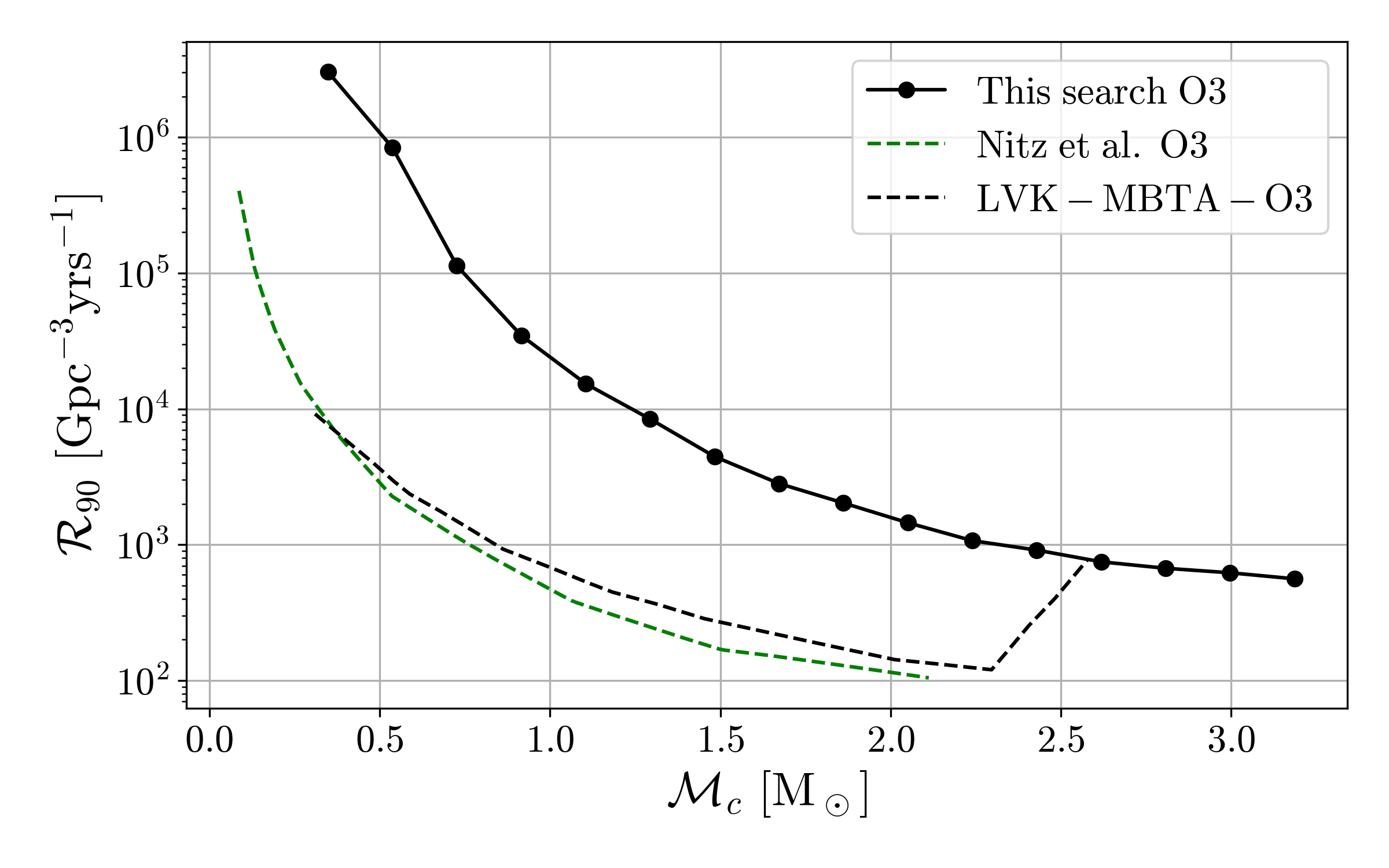
Figure 11: The 90$\%$ confidence level upper limit on $\mathcal{R}_{\rm{90}}$ as a function of the chirp mass. Our result (solid line) is compared with matched-filtering based results Abbott et al. (2022b); Nitz and Wang (2022) (dashed lines).

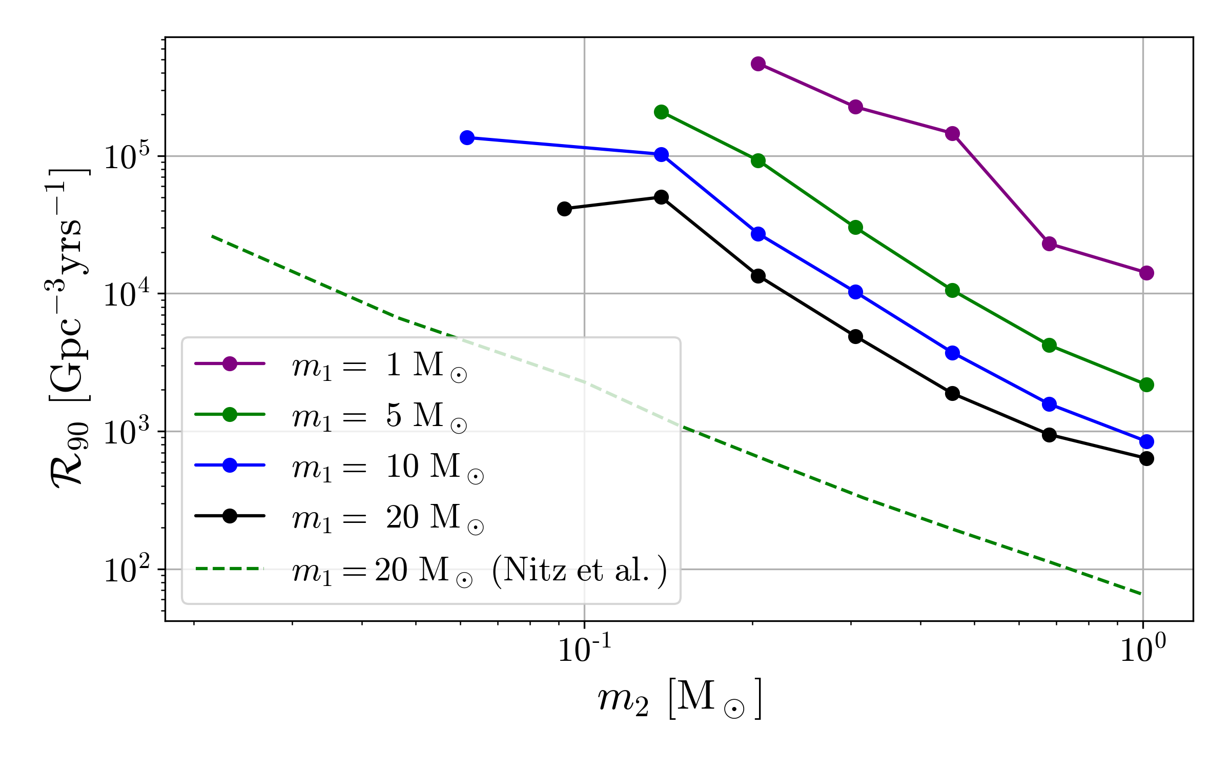
Figure 12: The 90$\%$ confidence level upper limit on $\mathcal{R}_{\rm{90}}$ as function of $m_{2}$ in different $m_{1}$ regions. Our result (solid lines) is compared with Nitz et al. results Nitz and Wang (2022) (dashed line).

V Conclusions

We present the results on a search for compact binary coalescence events with asymmetric mass configurations with masses in the range $0.01~{}\rm{M\textsubscript{$\odot$}}$ and $1~{}\rm{M\textsubscript{$\odot$}}$ for the lighter object and between $1~{}\rm{M\textsubscript{$\odot$}}$ and $20~{}\rm{M\textsubscript{$\odot$}}$ for the heavier, using LIGO-Virgo O3 data and dedicated convoluted neural networks based on the analysis of frequency-time spectrograms. Different neural networks and combination of them are explored, involving the simultaneous use of several interferometers data. The scan over the O3 data results into no significant signal events found. The CNN approach for scanning the data is found to be much faster than traditional matched-filtering based pipelines. The CNN results are translated into 90$\%$ confidence level upper limits on the merger rates as a function of the mass parameters of the binary system for events within $z<0.06$ and for the trained range. Although the results do not improve other bounds using matched-filtering techniques, partially due to the limited observation time considered, the CNN approach allows for effectively extending the search towards larger chirp masses.

References

- Abbott et al. (2016a) B. Abbott et al. (LIGO Scientific Collaboration, Virgo Collaboration), Physical Review Letters 116 (2016a), ISSN 1079-7114.
- Abbott et al. (2019a) R. Abbott et al. (LIGO Scientific Collaboration, Virgo Collaboration), Physical Review X 9, 031040 (2019a), ISSN 21603308.
- Abbott et al. (2020a) R. Abbott et al. (LIGO Scientific Collaboration, Virgo Collaboration), Physical Review X 11, 021053 (2020a).
- Abbott et al. (2021) R. Abbott et al. (LIGO Scientific Collaboration, Virgo Collaboration, KAGRA Collaboration), 48, 147 (2021).
- Abbott et al. (2020b) B. P. Abbott et al. (LIGO Scientific Collaboration, Virgo Collaboration), Class. Quant. Grav. 37, 055002 (2020b), eprint 1908.11170.
- Cuoco et al. (2020) E. Cuoco, J. Powell, M. Cavaglià, K. Ackley, M. Bejger, C. Chatterjee, M. Coughlin, S. Coughlin, P. Easter, R. Essick, et al., Machine Learning: Science and Technology 2, 011002 (2020).
- Gabbard et al. (2018) H. Gabbard, M. Williams, F. Hayes, and C. Messenger, Phys. Rev. Lett. 120, 141103 (2018).
- George and Huerta (2017) D. George and E. A. Huerta, Deep neural networks to enable real-time multimessenger astrophysics (2017), eprint 1701.00008.
- Gebhard et al. (2019) T. D. Gebhard, N. Kilbertus, I. Harry, and B. Schölkopf, Physical Review D 100 (2019), ISSN 2470-0029.
- George and Huerta (2018) D. George and E. A. Huerta, Physics Letters, Section B: Nuclear, Elementary Particle and High-Energy Physics 778, 64 (2018), ISSN 03702693.
- Menéndez-Vázquez et al. (2021) A. Menéndez-Vázquez, M. Kolstein, M. Martínez, and L. M. Mir, Phys. Rev. D 103, 062004 (2021).
- Razzano and Cuoco (2018) M. Razzano and E. Cuoco, Classical and Quantum Gravity 35, 095016 (2018), ISSN 1361-6382.
- Biswas et al. (2013) R. Biswas, L. Blackburn, J. Cao, R. Essick, K. A. Hodge, E. Katsavounidis, K. Kim, Y.-M. Kim, E.-O. Le Bigot, C.-H. Lee, et al., Physical Review D 88 (2013), ISSN 1550-2368.
- Cavaglia et al. (2019) M. Cavaglia, K. Staats, and T. Gill, Communications in Computational Physics 25 (2019), ISSN 1815-2406.
- Hawking (1971) S. Hawking, Mon. Not. Roy. Astron. Soc. 152, 75 (1971).
- Carr and Hawking (1974) B. J. Carr and S. W. Hawking, Mon. Not. Roy. Astron. Soc. 168, 399 (1974).
- Hütsi et al. (2019) G. Hütsi, M. Raidal, and H. Veermäe, Phys. Rev. D 100, 083016 (2019).
- Hütsi et al. (2021) G. Hütsi, M. Raidal, V. Vaskonen, and H. Veermäe, JCAP 03, 068 (2021), eprint 2012.02786.
- D’Amico et al. (2018) G. D’Amico, P. Panci, A. Lupi, S. Bovino, and J. Silk, Mon. Not. Roy. Astron. Soc. 473, 328 (2018), eprint 1707.03419.
- Khlopov (2010) M. Y. Khlopov, Research in Astronomy and Astrophysics 10, 495 (2010).
- Belotsky et al. (2014) K. Belotsky, A. Dmitriev, E. Esipova, V. Gani, A. Grobov, M. Y. Khlopov, A. Kirillov, S. Rubin, and I. Svadkovsky, Modern Physics Letters A 29, 1440005 (2014).
- Shandera et al. (2018) S. Shandera, D. Jeong, and H. S. G. Gebhardt, Phys. Rev. Lett. 120, 241102 (2018).
- Kouvaris and Tinyakov (2011) C. Kouvaris and P. Tinyakov, Phys. Rev. D 83, 083512 (2011), eprint 1012.2039.
- Kaup (1968) D. J. Kaup, Phys. Rev. 172, 1331 (1968).
- Guo et al. (2019) H.-K. Guo, K. Sinha, and C. Sun, Journal of Cosmology and Astroparticle Physics 2019, 032 (2019).
- Colpi et al. (1986) M. Colpi, S. L. Shapiro, and I. Wasserman, Phys. Rev. Lett. 57, 2485 (1986).
- Abbott et al. (2022a) R. Abbott et al. (LIGO Scientific Collaboration and Virgo Collaboration), Phys. Rev. Lett. 129, 061104 (2022a).
- Nitz and Wang (2022) A. H. Nitz and Y.-F. Wang, Phys. Rev. D 106, 023024 (2022).
- Abbott et al. (2022b) B. Abbott et al. (LIGO Scientific Collaboration, Virgo Collaboration, KAGRA Collaboration), arXiv preprint arXiv:2212.01477 (2022b).
- Nitz and Wang (2021a) A. H. Nitz and Y.-F. Wang, The Astrophysical Journal 915, 54 (2021a).
- Nitz et al. (2021) A. H. Nitz, Y.-F. Wang, et al., Physical Review Letters 126, 021103 (2021).
- Phukon et al. (2021) K. S. Phukon, G. Baltus, S. Caudill, S. Clesse, A. Depasse, H. Fong, S. J. Kapadia, R. Magee, and A. J. Tanasijczuk, arXiv preprint arXiv:2105.11449 (2021).
- Abbott et al. (2019b) R. Abbott et al. (The LIGO Scientific Collaboration, Virgo Collaboration), Phys. Rev. Lett. 123, 161102 (2019b).
- The LIGO Scientific Collaboration (2021) The LIGO Scientific Collaboration, Classical and Quantum Gravity 38, 135014 (2021).
- Virgo Collaboration (2022) Virgo Collaboration, arXiv preprint arXiv:2205.01555 (2022).
- Usman et al. (2016) S. A. Usman, A. H. Nitz, I. W. Harry, C. M. Biwer, D. A. Brown, M. Cabero, C. D. Capano, T. D. Canton, T. Dent, S. Fairhurst, et al., Classical and Quantum Gravity 33, 215004 (2016), ISSN 0264-9381.
- Nitz et al. (2017) A. H. Nitz, T. Dent, T. Dal Canton, S. Fairhurst, and D. A. Brown, The Astrophysical Journal 849, 118 (2017).
- Nitz et al. (2020) A. Nitz, I. Harry, D. Brown, C. M. Biwer, J. Willis, T. Dal Canton, C. Capano, L. Pekowsky, T. Dent, A. R. Williamson, et al., Zenodo (2020).
- Husa et al. (2016) S. Husa, S. Khan, M. Hannam, M. Pürrer, F. Ohme, X. J. Forteza, and A. Bohé, Physical Review D 93, 044006 (2016), ISSN 24700029.
- Khan et al. (2016) S. Khan, S. Husa, M. Hannam, F. Ohme, M. Pürrer, X. J. Forteza, and A. Bohé, Physical Review D 93 (2016), ISSN 24700029.
- Abbott et al. (2020c) B. P. Abbott et al. (LIGO Scientific Collaboration, Virgo Collaboration), Classical and Quantum Gravity 37, 055002 (2020c).
- Brown (1991) J. C. Brown, The Journal of the Acoustical Society of America 89, 425 (1991).
- Brown and Puckette (1992) J. C. Brown and M. S. Puckette, The Journal of the Acoustical Society of America 92, 2698 (1992).
- Schörkhuber and Klapuri (2010) C. Schörkhuber and A. Klapuri, in 7th sound and music computing conference, Barcelona, Spain (2010), pp. 3–64.
- Ioffe and Szegedy (2015) S. Ioffe and C. Szegedy, Batch normalization: Accelerating deep network training by reducing internal covariate shift (2015), eprint 1502.03167.
- Menéndez-Vázquez et al. (2021) A. Menéndez-Vázquez, M. Kolstein, M. Martínez, and L. M. Mir, Physical Review D 103, 1 (2021), ISSN 24700029.
- He et al. (2016a) K. He, X. Zhang, S. Ren, and J. Sun, in Proceedings of the IEEE conference on computer vision and pattern recognition (2016a), pp. 770–778.
- He et al. (2016b) K. He, X. Zhang, S. Ren, and J. Sun, in European conference on computer vision (Springer, 2016b), pp. 630–645.
- Kingma and Ba (2014) D. P. Kingma and J. L. Ba, 3rd International Conference on Learning Representations, ICLR 2015 - Conference Track Proceedings (2014).
- Ruder (2016) S. Ruder, arXiv preprint arXiv:1609.04747 (2016).
- Goodfellow et al. (2016) I. Goodfellow, Y. Bengio, and A. Courville, Deep learning (MIT press, 2016).
- Abadi et al. (2016) M. Abadi, P. Barham, J. Chen, Z. Chen, A. Davis, J. Dean, M. Devin, S. Ghemawat, G. Irving, M. Isard, et al., in 12th USENIX symposium on operating systems design and implementation (OSDI 16) (2016), pp. 265–283.
- Abbott et al. (2016b) R. Abbott et al. (The LIGO Scientific Collaboration, Virgo Collaboration), Physical Review Letters 116, 061102 (2016b), ISSN 0031-9007.
- Abbott et al. (2005) R. Abbott et al. (The LIGO Scientific Collaboration, Virgo Collaboration), Physical Review D - Particles, Fields, Gravitation and Cosmology 72, 23 (2005), ISSN 15507998.
- Littenberg et al. (2016) T. B. Littenberg, J. B. Kanner, N. J. Cornish, and M. Millhouse, Physical Review D 94, 044050 (2016), ISSN 24700029.
- Lee et al. (2021) Y. S. C. Lee, M. Millhouse, and A. Melatos, Physical Review D 103, 062002 (2021), ISSN 24700029.
- Tiwari (2018) V. Tiwari, Classical and Quantum Gravity 35, 145009 (2018).
- Nitz and Wang (2021b) A. H. Nitz and Y. F. Wang, Physical Review Letters 127, 151101 (2021b), ISSN 10797114.