Hierarchical Decompositions and Termination Analysis
for Generalized Planning

Abstract

This paper presents new methods for analyzing and evaluating generalized plans that can solve broad classes of related planning problems. Although synthesis and learning of generalized plans has been a longstanding goal in AI, it remains challenging due to fundamental gaps in methods for analyzing the scope and utility of a given generalized plan. This paper addresses these gaps by developing a new conceptual framework along with proof techniques and algorithmic processes for assessing termination and goal-reachability related properties of generalized plans. We build upon classic results from graph theory to decompose generalized plans into smaller components that are then used to derive hierarchical termination arguments. These methods can be used to determine the utility of a given generalized plan, as well as to guide the synthesis and learning processes for generalized plans. We present theoretical as well as empirical results illustrating the scope of this new approach. Our analysis shows that this approach significantly extends the class of generalized plans that can be assessed automatically, thereby reducing barriers in the synthesis and learning of reliable generalized plans.

1 Introduction

Enabling autonomous agents to learn and represent generalized knowledge that can be used to solve multiple related planning problems is a longstanding goal in AI. The ability to create transferrable, generalized plans that can solve large classes of sequential decision making problems has long been recognized as essential in achieving this goal. However, research on the problem has been limited due to technical challenges in analyzing generalized plans. The problem of determining whether an arbitrary generalized plan is useful – i.e., whether it can be “transferred” to solve a desired class of problem instances is equivalent to determining whether a generalized plan terminates, which is undecidable in general. This significantly limits approaches for computing generalized plans: the absence of an effective evaluation function precludes computationally popular approaches for learning from past data as well as methods for synthesizing and improving candidate generalized plans. This reduces not only the robustness of algorithms for computing generalized plans but also the reliability of the computed generalized plans.

This paper presents a new, hierarchical approach for assessing the utility of a generalized plan. Since reachability of a desired goal state while executing a generalized plan can be reduced to determining termination, we focus on methods for determining termination. Our main contribution is a new conceptual framework and proof technique that can be used to design and validate algorithms for analyzing the reachability and termination properties of generalized plans. We draw upon insights from classic results in graph theory to create a hierarchical decomposition of a given generalized plan. This decomposition facilitates more general termination analysis than is possible using prior work. Although the problem of termination for generalized plans is undecidable in general, we show that in practice, the methods developed this paper can determine termination for broad classes of generalized plans that are beyond the scope of existing methods. This approach can also be used in popular generate-and-test driven paradigms for generalized planning where candidate generalized plans can be synthesized or learned from examples and pruned or refined on the basis of reachability analysis facilitated using the presented methods.

Advances in determining termination for limited classes of generalized plans (?, ?, ?) have led to immense progress in the field (e.g., ? (?); ? (?); ? (?); a more complete survey is presented in the next section). We expect that methods for more general methods for analyzing generalized plans will further enable continued breakthroughs in the field.

Prior work on theoretical aspects of generalized planning relies upon strong assumptions that restrict the structure of generalized plans, or limit the permitted actions to “qualitative” actions that cannot capture general forms of behavior. The framework developed in this paper goes beyond these limitations. It offers a sound but non-complete test of termination for generalized plans with arbitrary structures and actions that can increment or decrement variables by specific amounts in non-deterministic or deterministic control structures. Sound and complete methods for termination assessment of generalized plans are not possible, due to equivalence with the halting problem for Turing machines. Our framework supports counter-based actions that can express the full range of structured behaviors including arbitrary Turing machines. They can express changes in Boolean state variables as well as changes in higher-order state properties or features (e.g., the number of packages that still need to be delivered in logistics planning problems). Prior work on generalized planning has established that such counter-based representations capture the essence of generalized plans as needed for analysis of their utility (?, ?) as well as for synthesis of generalized plans and policies (?, ?).

The main new insight in this paper is that classic results in graph theory can be used to decompose an arbitrary generalized plan, expressed as a finite-state machine, into a finite hierarchy of generalized plans with a desirable property: the structure of generalized plans necessarily decreases in complexity as one descends in the hierarchy. This allows us to inductively build a new form of termination argument for a parent generalized plan in the hierarchy by composing termination arguments for its children generalized plans. Theoretical analysis and empirical results show that this method effectively addresses a broad class of generalized plans that were not amenable to existing approaches.

The rest of this paper is organized as follows. Sec. 2 presents a survey of related work on the topic followed by our formal framework and the problem setting (Sec. 3). Sec. 4 presents our new algorithmic framework for the analysis of generalized plans. This is followed by theoretical analysis illustrating the new proof techniques that this approach enables along with our key theoretical results on the soundness of the presented algorithm (Sec. 5.1) as well as our empirical analysis (Sec. 5.2). Sec. 6 presents our conclusions and directions for future work.

2 Related Work

Early work by ? (?) articulated the value of planning with iterative constructs and the challenges of proving that such constructs would terminate (or equivalently, achieve the desired goals) upon execution. This work focused on settings where problem classes are defined by varying a single numeric planning parameter. Levesque showed that this parameter could be used to build iterative constructs. He argued that rather than attempting to assess or prove the termination of such plans, asserting weaker guarantees could lead to computationally pragmatic approaches. Levesque proposed validation of computed iterative plans up to a certain upper bound on the single numeric planning parameter. To the best of our knowledge, this work constitutes the first clear articulation of the value and challenges of computing plans with loops using AI planning methods.

2.1 Counter-Based Models for Generalized Planning

? (?) showed that counters based on logic-based properties could be used to create numeric features, e.g., the number of cells that need to be visited in a grid exploration task. Such features can help identify useful iterative structures and compute “generalized plans”. Furthermore, the team showed that counter-based models for generalized planning could be used to determine whether a computed generalized would terminate and reach the goal. These methods were used to compute generalized plans with simple loops. The plan synthesis process ensured provable correctness and for a broad class of problems, the computed plans were guaranteed to solve infinitely many problem instances involving arbitrary numbers of counters. ? (?) showed that determining termination for plans featuring iteration over a single numeric planning parameter is decidable. In subsequent work, ? (?) showed that the problem of identifying useful cyclic control structures in generalized plans could be studied using foundational models of computation such as abacus programs by transforming the planning-domain actions into equivalent operations that changed counters corresponding to logic-based state properties. The team developed algorithms for determining termination and graph-theoretic characterizations of generalized plans that could be assessed for termination despite the general incomputability of the problem (?). These methods were also used to develop directed search and learning techniques for generalized planning (?).

In practice, the main technical problems in determining whether a generalized plan is “useful” is that it is difficult to construct termination arguments for complex terminating generalized plans: the set of generalized plans that can be proved to be terminating is a small subset of the set of terminating generalized plans. Although the strict subset relationship must hold due to equivalence of this problem with the halting problem, it is essential to develop new approaches that identify and push the boundary of decidability further.

The framework of qualitative numeric planning (QNP, ? (?)) extended the counter-based model for generalized planning further to address these limitations. This framework introduces action semantics under which the set of terminating generalized plans reduces to generalized plans for which the “Sieve” algorithm can assert termination. The QNP framework is broadly applicable in practice and yet insufficient to express Turing machines. A more formal comparison of termination under qualitative and deterministic semantics is presented in Sec. 4.1. QNPs were later extended to more general settings along with analysis of their expressiveness and a more general version of the Sieve algorithm (?). ? (?) showed that the analysis conducted by the Sieve algorithm for QNP problems can also be viewed as a fully observable non-determinstic (FOND) planning process. These foundational formulations of generalized planning have been extended in several directions. ? (?) develop connections between generalized planning and LTL synthesis; ? (?) analyzes the relationships between various correctness criteria in stochastic and non-deterministic settings.

2.2 Meta-Level Planning for Computing Generalized Plans

The theoretical advances discussed above have been accompanied with numerous advances in approaches for computing generalized plans. ? (?) showed that the computation of finite-state controllers for some classes of planning problems could be reduced to planning by creating meta-level planning domains whose actions involved the addition or deletion of edges in a controller. These finite-state controllers were observed to have good generalization capabilities. Several threads of research have developed this approach of creating meta-level planning problems that synthesize generalized plans in the form of controllers (?, ?, ?). ? (?) present algorithms for computing hierarchical generalized plans that include subroutines and are guaranteed to solve an input set of finitely many planning problems. The planning domains used in this reduction include actions that construct components of hierarchical finite-state controllers as well as validate the resulting controllers on the input problem set. This paradigm of evaluation using a finite validation set has been developed along multiple directions to utilize finite sets of positive examples as well as negative examples indicating undesired outcomes of plan execution (?) and with finite validation sets for use in a general heuristic search process for computing generalized plans (?, ?).

2.3 Broader Applications

Foundations of generalized planning discussed above have also enabled broader advances in sequential decision making. As noted above, state representations based on counters capturing the numbers of objects that satisfy various properties were developed originally for identifying and analyzing iterative structures for generalized plans. They have since been found to be useful also for computing generalized, domain-wide planning knowledge. Such methods have been utilized for learning and synthesis of generalized knowledge for sequential decision making in the form of general sketches and policies for planning (?, ?, ?, ?), for learning neuro-symbolic generalized heuristics for planning (?) and neuro-symbolic generalized Q-functions for reinforcement learning in stochastic settings (?), as well as for few-shot learning of generalized policy automata for stochastic shortest path problems (?). In the terminology of metrics for generalized planning presented by ? (?), these methods compute generalized plans that have a relatively higher cost of instantiation that is still much lesser lower than that of planning from scratch. On the other hand, these methods provide a significantly higher domain coverage than that of an optimized generalized plan. These directions of research bridge the gap between generalized planning and lifted sequential decision making (?, ?, ?). Other approaches for learning generalized knowledge include approaches for learning general policies in a relational language (?, ?, ?), learning heuristics for solving multiple planning problems (?, ?, ?, ?, ?) as well as generalized neural policies for relational MDPs (?).

3 Problem Formulation

We use a foundational but powerful representation where all variables are numeric variables with $\mathbb{N}$ as their domains. Let $\mathcal{V}$ be the set of such variables. A concrete state is an assignment that maps each variable in $\mathcal{V}$ to a value in that variable’s domain. We denote the set of all possible concrete states as $\mathcal{S}_{\mathcal{V}}$. The value of a variable $x$ in a state $s\in\mathcal{S}_{\mathcal{V}}$ is denoted as $s(x)$. In this paper we use the unqualified term “state” to refer to concrete states.

Definition 1.

An action consists of a precondition, which maps each variable in $\mathcal{V}$ to a union of intervals for that variable, and a set of action effects, $\emph{effects}(a)$. Each member of $\emph{effects}(a)$ is of the form $\oplus x$ or $\ominus x$, where $x\in vars$; $\emph{effects}(a)$ must include at most one occurrence of each variable in $\mathcal{V}$.

Prior work in generalized planning considers three types of interpretations of $\oplus,\ominus$ that correspond to popular frameworks in the literature (?). We focus on deterministic and qualitative semantics in this work:

Deterministic semantics

Under deterministic semantics, each occurrence of $\oplus$ ($\ominus$) in an action effect is interpreted as an increment (decrement) by a fixed discrete quantity. E.g., an action’s effects may include $x_{1}+1,x_{2}-5,x_{3}+1$ for variables $x_{1},x_{2},$ and $x_{3}$. $a(s_{1})$ is defined as the unique state $s_{2}$ such that for every $x\in\mathcal{V}$ if $x+i$ is an effect of $a$, $s_{2}(x)=s_{1}(x)+i$ and if $x-j$ is an effect of $a$ then $s_{2}(x)=s_{1}(x)-j$. $s_{2}(x)=s_{1}(x)$ for all $x$ that don’t occur in effects of $a$. The special case of deterministic semantics where for every variable $x$, $\oplus x=x+1$ and $\ominus x=x-1$ yields formulations close to abacus programs (?).

Although we will focus on deterministic semantics in this paper, we introduce qualitative semantics below in order to compare and contrast our approach with prior work.

Qualitative semantics

Under qualitative semantics, each occurrence of $\oplus$ ($\ominus$) is interpreted as an increase (decrease) by a non-deterministic amount. The amount of change caused due to each $\ominus$ is such that in any execution, a finite sequence of consecutive $\ominus x$ effects is sufficient to reduce $x$ to zero for any finite value of $x$. This is defined formally as follows (?). Let $\epsilon>0$ be an unknown constant that is fixed for an entire execution. Formally, the effect of $\oplus x$ is to non-deterministically increase $x$ by $\delta_{\oplus}$, where $\delta_{\oplus}\in[\epsilon,\infty)$. The effect of $\ominus x$ is to non-deterministically decrease $x$ by $\delta_{\ominus}$ such that for every execution, $\delta_{\ominus}\in[\emph{min}\{\epsilon,x\},x]$.

To accommodate a unified discussion of these semantics, we will use the notation $a(s)$ to refer to the set of states that can result upon execution of $a$ in $s$ and clarify the semantics being used as required.

Definition 2.

A planning domain $\langle\mathcal{V},\mathcal{A}\rangle$ consists of a finite set of variables $\mathcal{V}$, and a finite set of actions $\mathcal{A}$ over $\mathcal{V}$.

Definition 3.

A planning problem $\langle\mathcal{D},s_{o},g\rangle$ consists of a planning domain $\mathcal{D}=\langle\mathcal{V},\mathcal{A}\rangle$, a concrete state $s_{0}$ and a goal mapping $g$ from $V\!\!\subseteq\!\mathcal{V}$ to intervals in $\mathbb{N}$.

3.1 Solutions to Planning Problems

At every step, the action to be performed for solving a given planning problem may depend on finite representations of the history of executed actions and received observations. Such solutions can be represented as graph-based generalized plans (?), or as finite-state controllers (?, ?). Formally, we use the following notion of a finite-state controller based policy.

Definition 4.

Let $\mathcal{D}=\langle\mathcal{V},\mathcal{A}\rangle$ be a planning domain and let $\Psi$ be the set of formulas over propositions of the form $x_{i}\gtreqless l_{i}$ where $x_{i}\in\mathcal{V}$ and $l_{i}\in\mathbb{N}$. A finite-memory policy (FMP) for $\mathcal{D}$ is defined as $\langle Q,q_{0}\in Q,\delta,\kappa\rangle$ where $Q$ is a finite set of control states, $q_{0}$ is the starting state, $\delta\subseteq Q\times Q$ is the transition relation and $\kappa:\delta\rightarrow\Psi\times\mathcal{P}(\mathcal{A})$ is a labeling function that labels each directed edge between control states with an execution condition and a set of actions.

Throughout this paper we will assume that execution conditions on FMP edges include as defaults the non-negativity condition $x_{i}\geq 0$, for all $x_{i}\in\mathcal{V}$. In practice each variable can have a different lower bound as the methods presented in this paper depend only on the existence of default bounds on variables. The technical results presented in this paper can be easily extended to settings where $x_{i}$’s also have upper bounds. They can also be extended to settings where $x_{i}$’s are bounded only above by replacing arguments about actions’ effects on decreasing variables with their effects on increasing variables and including the upper bounds as default execution conditions.

This representation generalizes the existing forms of policies used with qualitative as well as deterministic semantics. When needed for clarity, we will use the term “control states” or “qstates” to refer to the states of an FMP policy and “problem states” to refer to the states defined by a planning domain.

Execution of an FMP starts with $q_{0}$. At any stage during the execution where the problem state is $s_{1}\in\mathcal{S}_{\mathcal{V}}$ and the FMP is in control state $q_{1}\in Q$, the agent can execute any action $a$ s.t. there exists a control state $q_{2}\in Q$ for which $\kappa(q_{1},q_{2})=(\psi,A)$, $a\in A$, and $s_{1}\models\varphi$. Following such an action, the FMP’s control state becomes $q_{2}$. Execution stops at a state $s$ if the FMP is in a control state $q$ that has no outgoing edges whose execution condition is consistent with $s$. Thus, an FMP terminates if its execution reaches a terminal control state, or if it reaches a control state such that none of its outgoing edge conditions is satisfied in the current problem state.

An FMP is said to be deterministic iff for every $q\in Q$, the set of outgoing edges are labeled with mutually inconsistent execution conditions and singleton action sets so that at most one action is possible at every step during execution.

Existing notions of qualitative policies are closely related with FMPs. For instance, an abstract policy $\pi$ (?, ?) that maps abstract states to actions can be expressed as FMPs with one control state $q_{0}$ and the labeling function $\kappa(q_{0},q_{0})=\{(\tilde{s},\{a\}):\pi(\tilde{s})=a\}$. “Sketch” based generalized policies (?) can be expressed as FMPs where the edge label consists of a condition $\psi$ but $\mathcal{P}(A)$ is replaced by a set of integers denoting changes in the values of a subset of the variables in $\mathcal{V}$. An edge in such a sketch can be taken if the agent executes a sequence of actions that causes the corresponding change. Since the framework for analysis developed in this paper considers the changes induced by FMP edges rather than the action names, it offers a promising direction for analyzing properties of sketch based policies as well.

We say that an FMP has a well-defined set of terminal states $H\subseteq Q$ if the states in $H$ have no outgoing edges and when started with any state in $s\in\mathcal{S}$, execution continues until $H$ is reached. Execution of policies that do not have well-defined halt states can end in arbitrary control states when the policy does not have any outgoing edges corresponding to the current state of the problem. This represents situations that are in some sense unforeseen according to the FMP and is especially common with FMPs that are generated through learning over a limited training dataset.

3.1.1 Solution Properties

Given an initial state $s_{0}\in\mathcal{S}_{\mathcal{V}}$, an execution of an FMP policy $\langle Q,q_{0}\in Q,\delta,\kappa\rangle$ is defined as a sequence $(q_{0},s_{0}),a_{0},(q_{1},s_{1}),a_{1},\ldots$ such that $\kappa(q_{i},q_{i+1})=(\varphi_{i},A_{i})$, $a_{i}\in A_{i}$, $s_{i+1}\in a_{i}(s_{i})$ and $s_{i}\models\varphi_{i}$. Two criteria over the set of executions possible under an FMP policy can be used to define the quality of the policy. If a policy $\Phi$ is such that every execution of $\Phi$ stops after a finite number of steps when started with an initial state $s_{0}$, we say that $\Phi$ terminates for $s_{0}$. If $\Phi$ terminates for all $s\in\mathcal{S}_{\mathcal{V}}$, we say that it is a terminating policy. A terminating policy whose execution ends only at states satisfying the goal condition $g$ of the given domain is said to be goal achieving.

4 Determining Termination of Finite Memory Policies

Recall that we adopt the fail-stop mode of execution semantics for FMPs, where execution stops if the current control state has no outgoing edges consistent with the current problem state. As discussed under related work, several algorithms for generalized planning learn or iterate over multiple solution structures that can be expressed in the form of FMPs. To evaluate the utility of a candidate FMP as a solution, we need to consider two key properties: reachability and termination. Ideally, we would want to establish that every execution of an FMP reaches the goal in a finite number of steps for all the initial problem states of interest.

It is well known that decision problems of termination and reachability can be reduced to each other. Prior work (?, ?) shows that this is undecidable in general, because showing that every execution terminates in a finite number of steps is equivalent to the halting problem for Turing machines. In this section we present our new approach for hierarchically decomposing and analyzing FMPs to determine termination.

We begin with a formal analysis of the relationship between qualitative semantics and deterministic semantics with respect to termination analysis.

4.1 Termination Under Qualitative and Deterministic Semantics

Background on the Sieve family of algorithms

The Sieve family of algorithms (?, ?) are sound and complete tests of termination under qualitative semantics, but only sound for deterministic semantics. Although the correctness of these algorithms was proved for abstract policies and transition graphs, the results carry over in a straightforward manner to FMPs. The Sieve algorithm (?) conducted this analysis for variables bounded below. The Progress-Sieve algorithm (?) generalized this intuition to settings with variables with discrete observable levels and upper or lower bounds, and is listed here as Alg. 1 for ease of reference.

Input: $g=\emph{ts}(\pi,\tilde{s_{I}})$

1 Remove all edges $e$ of $g$ that have a progress variable w.r.t. their SCCs

2if no edge was removed then

      3 Return “Non-terminating”

4for $g^{\prime}\in\emph{SCCs-of(g)}$ do

      5 if Progress-Sieve($g^{\prime}$)= “Non-terminating” then

            6Return “Non-terminating”

      

7Return “Terminating”

Algorithm 1 (Progress-Sieve) abstract policy termination test (?)​​

Intuitively, this class of algorithms operate as follows: for each strongly connected component (SCC), the algorithm identifies “progress” variables that are changed in only one direction (positively or negatively): the direction in which they are bounded (above or below, respectively). Progress-Sieve removes edges modifying such a variable if the edge moves it towards the bound on the variable. If any edge was removed, the entire process is repeated. This continues until either the graph is left with no strongly connected components and the policy is reported as terminating, or strongly connected components remain, but no progress variables are found and the policy is reported as non-terminating.

The following natural result relating termination in deterministic and qualitative settings is useful to list out for completeness:

Proposition 1.

Let $\Phi=\langle Q,q_{0},\delta,\kappa\rangle$ be an FMP. If $\Phi$ terminates for $s_{0}\in\mathcal{S}_{\mathcal{V}}$ under qualitative semantics, then it must terminate for $s_{0}$ under deterministic semantics.

The proof is straightforward because increments and decrements by a constant are a special case of qualitative effects. If $\Phi$ does not terminate under such effects, then it clearly cannot terminate under the qualitative semantics with the same action instantiations.

However, the other direction is not true: termination under deterministic semantics does not imply termination under qualitative semantics, as shown in the following counter-example.

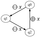
Figure 1: An FMP that terminates under deterministic semantics ($\oplus=+1$ and $\ominus=-1$) but not under qualitative semantics (see Example 1).

Example 1.

Let $\Phi$ be an FMP with three qstates $q_{0},q_{1}$ and $q_{2}$ as shown in Fig. 1. $\Phi$ is a terminating policy under deterministic semantics where $\ominus x=x-1,\oplus x=x+1$ (due to the default edge conditions on non-negativity). However, it is not a terminating policy under qualitative semantics because the $\ominus$’es may be small enough to be overwhelmed by the $\oplus$ in every iteration of the cycle.

This example also shows why we are able to develop sound and complete tests for termination for qualitative numeric planning: under qualitative semantics, actions are sufficiently imprecise that the effective class of terminating policies reduces to match the analysis conducted by the Sieve family of algorithms. This also limits the types of behaviors that can be expressed using qualitative semantics. ? (?) study this boundary of expressiveness further and identify conditions under which policies with qualitative semantics are insufficient for expressing solutions to planning problems.

4.2 A Hierarchical Framework for Termination Analysis

While the Sieve algorithms discussed above constitute an efficient and sound method for identifying a restricted class of terminating FMPs, they have somewhat obvious limitations when considering deterministic semantics, as illustrated in Example 1. Under deterministic semantics with default edge conditions enforcing non-negativity, the execution of this SCC is guaranteed to stop in a finite number of steps regardless of the initial value of the variable being changed by its actions. However, Sieve algorithms cannot determine that this SCC terminates because it does not have a progress variable. This is consistent with completeness under qualitative semantics, which would allow the $\oplus$ operation to increase the variable arbitrarily, although it misses rather obvious patterns of termination under deterministic semantics.

Example 1 lends some intuition about the type of reasoning that is required to develop a more general algorithm for determining termination under deterministic semantics. Instead of requiring a non-monotonic decrease over all edges in an SCC, we need a way to assess the net changes on a variable over execution segments that can be repeated indefinitely in an infinite execution that might occur when the FMP is interpreted as a finite automaton without edge conditions. However, reasoning about possible execution trajectories in an SCC becomes difficult when nested cycles are present: any number of iterations of one cycle may be interleaved with an arbitrary number of iterations of subsequences another cycle within the same SCC. A test for termination would have to assess all the infinitely many possible permutations of this form.

We formalize this intuition by first defining a richer notion of progress variables as follows. If variables are bounded above, a similar notion of increasing progress variables can be defined and the subsequent analysis can be extended to those cases. As with the default edge conditions, in this paper we focus on the setting where variables are bounded only from below. We focus on deterministic semantics in the rest of this paper.

Definition 5.

Let $\Pi$ be a set of paths in an FMP and let $\pi\in\Pi$. A variable $v$ is a net-decrease variable for a path $\pi$ w.r.t. $\Pi$ iff $v$ undergoes a net decrease in $\pi$ and $v$ does not undergo a net increase in any path in $\Pi$. We use $\Downarrow^{\pi}_{\Pi}$ to denote the set of all net-decrease variables for $\pi$ w.r.t $\Pi$ and extend this notation to define $\Downarrow_{\Pi}$ as the set of sets of net-decrease variables for all paths in $\Pi$: $\Downarrow_{\Pi}=\{\Downarrow^{\pi}_{\Pi}:\pi\in\Pi\}$.

Notice that each element of $\Downarrow_{\Pi}$ is a set. Thus if the number of non-empty sets in $\Downarrow_{\Pi}$ is the same as the cardinality of $\Pi$, then every path in $\Pi$ creates a net decrease in some variable that does not undergo a net increase by any path in $\Pi$. Intuitively, if $\Pi$ denotes the set of all possible paths in (including repetitions) in an SCC, and $\Downarrow_{\Pi}$ has no empty sets then execution cannot continue indefinitely within $\Pi$: every path creates a net decrease that cannot be undone in $\Pi$ and execution conditions include non-negativity. Unfortunately however, this intuition is computationally ineffectual because the set of possible execution paths (which can include multiple executions of SCCs) in a graph with SCCs is infinite.

4.2.1 Structures for Hierarchical Decomposition of FMPs

To push the envelope on determining whether an FMP will terminate, we need to be able to structure the possible executions of an SCC in an FMP. Intuitively, we wish to develop a bottom-up process that analyzes “inner” loops before moving on to “outer” loops that span the inner ones. Although this intuition is helpful, it is not sufficient because an infinite execution of an FMP can include infinitely many non-consecutive occurrences of non-cycles in the form of “bridge” paths and shortcuts through SCCs. We develop this intuition by building on McNaughton’s notion of analysis of a graph (?), which facilitates the construction of a directed tree over the components of an SCC. For clarity we will use Gruber’s version of this concept, formalized as Directed Elimination Trees (?). Let $G_{X}$ denote the subgraph of $G=(V,E)$ formed using the vertices $X\subseteq V$.

Definition 6.

A directed elimination tree (DET) for a non-trivially strongly connected digraph $G=(V,E)$ is a rooted tree $DET_{G}=(T_{V},T_{E})$ where $T_{V}\subseteq 2^{V}\times V$ with the root $\langle V,v\rangle$ such that $DET_{G}$ satisfies the following properties:

• If $\langle H,v\rangle\in T_{V}$, then $v\in H$

• There is no pair of distinct vertices of the form $\langle H,x\rangle$ and $\langle H,y\rangle$

• If $\langle H,v\rangle$ is a node in $T$ and $G_{H}\setminus\{v\}$ has $j\geq 0$ non-trivial SCCs $G_{1},\ldots,G_{j}$, then $\langle H,v\rangle$ has exactly $j$ children denoted as $ch(H,v)=\{\langle G_{1},v_{1}\rangle,\ldots,\langle G_{j},v_{j}\rangle\}$, for some $v_{i},\ldots,v_{j}\in V$.

If $\langle G,v\rangle$ is a node in a DET, we refer to $v$ as the elimination point for that node. We will use the concept of directed elimination trees with FMPs by interpreting an FMP as a graph in the usual manner of representing controllers as graphs. We will use FMPs and their graphs interchangeably and clarify the distinction when required for clarity. In general, an FMP will yield a directed elimination forest (DEF) consisting of one directed elimination tree for each strongly connected component in the FMP.

Example 2.

Fig. 2 (left) shows an example of an FMP with edge labels representing actions in deterministic semantics. This example was created by adding additional edges and edge labels to McNaughton’s classic example of a strongly connected digraph (?). In this example, edge conditions are the default non-negativity conditions. The right subfigure shows a DEF for the same FMP.

(a) Finite-memory policy $\Phi_{1}$

(b) Directed elimination forest $D_{\Phi_{1}}$for $\Phi_{1}$

Figure 2: A finite-memory policy and its directed elimination forest. Nodes in $D_{\Phi_{1}}$ are labeled $(V_{G},v)$ where $V_{G}$ is the set of vertices for the component $G$.

Directed elimination trees are closely related to cycle ranks (?). In fact, the minimal height of directed elimination trees for a graph is the cycle rank of that graph (?). Cycle ranks are closely related to multiple notions of the complexity of recurring patterns of behavior, e.g., the star-height of regular expressions.

Although the problem of computing a minimal directed elimination tree is equivalent to the problem of computing the cycle rank of a graph and is NP-complete, our algorithm does not require minimality. This is helpful because polynomial-time divide-and-conquer algorithm can be used to compute a directed elimination tree within a factor $O((log~{}n)^{3/2})$ of the minimal height. This result and a greater discussion of DETs for structural categorizations of computational complexity can be found at (?).

Termination Analysis Using DEFs

We now develop the formal concepts required to develop a stronger test for termination under deterministic concepts.

We wish to define an inductive, bottom-up process on the directed elimination tree to derive a set of net-progress variables for the entire SCC. To do this, we need to define the notion of a graph that considers sub-components as black boxes that are guaranteed to have net-progress variables. Let $\langle G,v\rangle$ be a node in a directed elimination tree for an FMP policy, with children nodes $\emph{ch}(G,v)=\{\langle G_{1},v_{1}\rangle,\ldots,\langle G_{k},v_{k}\rangle\}$. Recall that by definition this implies that $G$ is an SCC such that upon removing $v$, $G$ is left with SCCs $G_{1},\ldots,G_{k}$.

We define the quotient graph of $G$ w.r.t. $\emph{ch}(G,v)$ (denoted as $G|_{ch(G,v)}$) as the graph obtained by replacing each $G_{i}$ in $\emph{ch}(G,v)$ with a new component vertex $c_{i}$ while inheriting all the edges that led into, or out of $G_{i}$. Intuitively, $c_{i}$ encapsulates $G_{i}$ and $G|_{ch(G,v)}$ can be thought of as an SCC of rank 1 over $G_{i}$’s.

Example 3.

Fig. 3 shows the quotient graph $G|_{\{q4\_q5\_q6\_q7\},\{q0\_q1\}}$ for the root node of the non-trivial tree in the DEF from Fig. 2(b). Here $G$ is the subgraph of Fig. 2(a) induced by the qstates $\{q0,q1,q2,q3,q4,q5,q6,q7\}$. Since the root node $\langle G,q2\rangle$ has two children nodes, these subgraphs are replaced by component vertices in the quotient graph. Quotient graphs help simplify reasoning about possible executions of a FMP policy. For instance, this quotient graph indicates that any infinite execution of $\Phi_{1}$ that does not have an infinite suffix in $\{q4,q5,q6,q7\}$ and in $\{q0,q1\}$ (i.e., that does not have an infinite execution contained entirely within one of the two child components) must visit $q2$ infinitely often.

Figure 3: Quotient graph corresponding to the first node of the non-trivial tree in Fig. 2(b). Component vertices are labeled using the prefix c:.

The hierarchical sieve algorithm developed in this paper formalizes the intuition that if each path segment that can be executed infinitely often (while ignoring edge conditions) has a net-progress variable that is not increased by other inner loops, and the outer loop also has such a net-progress variable, then the SCC cannot be executed indefinitely when edge conditions are considered. More precisely, if $G|_{\emph{ch}(G,v)}$ and each $G_{i}\in\emph{ch}(G,v)$ has net-progress variables that are not increased by the other children of $G$ or by $G|_{\emph{ch}(G,v)}$ then $G$ itself has a net-progress variable, which implies that executions within $G$ must terminate or exit $G$. We develop this intuition by first computing a superset of paths (not necessarily complete cycles) that can be executed infinitely often when edge conditions are not considered.

Let $G^{0}_{\Phi}$ be the graph of an FMP $\Phi$ and let $\langle G,v\rangle$ be a node in the DEF of $G^{0}_{\Phi}=(V_{\Phi},E_{\Phi})$. Let $\Pi_{c}(G,v)$ denote the set of all cycle-paths in $G|_{\emph{ch}(G,v)}$: paths that start and end at $v$ and visit $v$ exactly twice. $\Pi_{c}(G,v)$ denotes cycles in $G|_{\emph{ch}(G,v)}$ that start and end at $v$. No such path can visit any node (qstate or component vertex) of $G|_{\emph{ch}(G,v)}$ other than $v$ twice because by definition of the elimination tree and $G|_{\emph{ch}(G,v)}$, removing $v$ from $G$ renders $G|_{\emph{ch}(G,v)}$ acyclic.

We also need to consider paths that go through $G$ without encountering any cycles. Let $I_{G}$ be the set of boundary vertices for edges that enter $G$, i.e., $\{v\in G:\emph{ there is a }w\in V_{\Phi}\setminus G\emph{ such that }\langle w,v\rangle\in E_{\Phi}\}$. Similarly, let $O_{G}$ be the set of boundary vertices for out-going edges from $G$. We define the set of through-paths for $G$, $\Pi_{io}(G,G^{0}_{\Phi})$, as the set of all cycle-free paths in $G$ that go from a vertex in $I_{G}$ to a vertex in $O_{G}$. Notice that this definition of through paths considers all of the vertices in $G$ while the $\Pi_{c}$ considers paths in $G|_{\emph{ch}(G,v)}$. Considering all through-paths in this manner allows for a more accurate algorithmic test for termination but this would be difficult to do while considering all possible combinations of cycles in G, with different possible numbers of iterations of each cycle. Thus we use quotient graphs to hierarchically structure the cycles into a more manageable framework. Let $\Pi(G,v)=\Pi_{io}(G,G^{0}_{\Phi})\cup\Pi_{c}(G,v)$.

Example 4.

Continuing with the running example, consider $G|_{\{q4\_q5\_q6\_q7\},\{q0\_q1\}}$, the quotient graph (Fig. 3) corresponding to the first node of the non-trivial DET shown in Fig.2(b). In this quotient graph the cycle paths are $(q2,q3,q2)$, $(q2,c\!:\!q4\_q5\_q6\_q7,q2)$ and $(q2,c\!:\!q0\_q1,q2)$. This node of the DET represents the qstates $\{q0,q1,q2,q3,q4,\allowbreak q5,q6,q7\}$. The only boundary vertex of the subgraph defined by these qstates is q6, and thus this subgraph has no through-paths. On the other hand, the subgraph defined by $\langle\{q4,q5,q6,q7\},q7\rangle$, a child node of $\langle\{q0,q1,q2,q3,q4,a5,q6,q7\},q2\rangle$, has $q4$ and $q6$ as boundary vertices and two through-paths: $(q4,q6)$ and $(q6,q4)$.

Using the notion of net-decrease variables for a set of paths (Def. 5), we define the net-decreased set for a node $\langle G,v\rangle$ in the elimination tree as the set of sets of net-decrease variables, with one set for each path in $\Pi(G,v)$. We denote this collection as $\Downarrow_{\Pi(G,v)}$ (abbreviated as $\Downarrow_{G,v}$). If any path in $\Pi(G,v)$ has no net-decrease variables, then the set of net decreased variables for that path is included in $\Downarrow_{G,v}$ as the empty set, $\emptyset$. In the same vein, we define possibly increased variables for $\langle G,v\rangle$, $\Uparrow_{G,v}$, as the set of variables that undergo a net increase in at least one path in $\Pi(G,v)$.

4.2.2 The GenSieve Algorithm

We now have all of the concepts required to present the main algorithm of this paper. Let $A\boxminus B$ denote the element-wise set-minus operation where $A$ is a set of sets and $B$ is a set: $A\boxminus B=\{x\setminus B:x\in A$}.

Let $G$ be the strongly connected graph of an FMP $\Phi$ and let $\langle G,v\rangle$ be the root node of its DET. If the input FMP has multiple strongly-connected components, we consider each component independently and prove termination by proving that each component terminates. GenSieve (Alg. 2) inductively derives an estimate $\hat{\Downarrow}_{G,v}$ ($\hat{\Uparrow}_{G,v}$) for the set of variables that could undergo a net negative (positive) change in a path in $\Pi(G,v)$ under default edge labels in $G$ as follows.

$$\hat{\Uparrow}_{G,v} = \Uparrow_{G,v}\cup\bigcup_{(G_{i},v_{i})\in\emph{ch}(G,v)}\hat{\Uparrow}_{G_{i},v_{i}}$$ (1)

$$\hat{\Downarrow}_{G,v} = \{\Downarrow_{G,v}\cup\bigcup_{(G_{i},v_{i})\in\emph{ch}(G,v)}\hat{\Downarrow}_{G_{i},v_{i}}\}\boxminus\hat{\Uparrow}_{G,v}$$ (2)

Since every directed elimination tree of a finite graph is finite and the base case is defined in closed form, this process must terminate after $h$ recursions where $h$ is the height of the directed elimination tree.

Input: FMP policy $G$

 /* IV: set of variables increased by a path in $\Pi(G)$ */

 /* pDV: set of sets of potential net-decrease variables per path in $\Pi(G)$ */

 /* DV: set of sets of net-decrease variables per path in $\Pi(G)$ */

 /* ZV: set of variables that undergo zero net change in a path in $\Pi(G)$ */

1progress=True

2 while progress=True do

      3 $DET_{G},\langle G,v\rangle\leftarrow$ DET of $G$ with root $\langle G,v\rangle$

      4 IV, ZV$\leftarrow$ BuildIncVars($G,v,DET_{G}$)

      

      5decreasedVars $\leftarrow$ BuildDecVars($G,v,DET_{G},\rm{\textit{IV}}$)

      6 decreasingEdges $\leftarrow$ edges that reduce decreasedVars not in ZV

      7 remove decreasingEdges from $G$

      8 if decreasingEdges $=\emptyset$ or $\{\}\not\in\emph{decreasedVars}$ then progress=False

      

9if $\{\}\in\emph{decreasedVars}$ then

      10 return “unknown”

else

      11 return “terminating”

Function BuildIncVars(G, v, DET)

      1 IV$\leftarrow\emptyset$; ZV$\leftarrow\emptyset$

      

      2foreach $\pi\in\Pi(G,v)$ do

            3 $\emph{IV}\leftarrow\emph{IV}\cup\{x:x\emph{ undergoes a net increase in }\pi\}$

            4 $ZV\leftarrow ZV\cup\{x:x\emph{ undergoes net zero change in }\pi\}$

            

      

      5foreach $\langle G_{i},v_{i}\rangle\in ch(G,v)$ do

             expand sets IV, ZV with output pair from BuildIncVars($G_{i},v_{i},DET$)

      

      6return IV, ZV

Function BuildDecVars(G, v, DET, IV)

      7 $pDV\leftarrow\emptyset$; $DV\leftarrow\emptyset$;

      

      8foreach $\pi\in\Pi(G,v)$ do

            9 $pDV\leftarrow pDV\cup\{\{x:x\emph{ undergoes net decrease in }\pi\}\}$

            

      

      10foreach $\langle G_{i},v_{i}\rangle\in ch(G,v)$ do  pDV $\leftarrow$ pDV $\cup$ BuildDecVars($G_{i},v_{i},DET,\rm{\textit{IV}}$)

      

      11$\emph{DV}\leftarrow\emph{pDV}\boxminus\emph{IV}$

      

      12return $DV$

      

Algorithm 2 GenSieve

Intuitively, GenSieve generalizes the intuition behind Sieve and Progress-Sieve algorithms. It attempts to identify every minimal path that can occur infinitely often in an execution in the form of $\Pi(G,v)$. The computation of every such path is difficult because of the variable nature of executions possible in FMPs with cycles, and the DET helps impose a hierarchical structure for extracting them.

GenSieve (Alg. 2) uses functions BuildIncVars and BuildDecVars to compute $\hat{\Uparrow}_{G,v}$ and $\hat{\Downarrow}_{G,v}$ using equations (1) and (2) respectively. In cases where $\hat{\Downarrow}_{G,v}$ includes an empty set, it means that there is a path in $\Pi(G,v)$ whose infinite execution cannot be ruled out yet. However, the computation of $\hat{\Downarrow}_{G,v}$ is conservative and can overestimate the impact of paths that increase variables. Some of these paths can become unreachable after finitely many steps of execution. To accommodate such situations, GenSieve computes the set of variables that are only decreased by elements of $\Pi(G,v)$ (lines 5-6). It then removes decreasingEdges, or edges that decrease such variables (line 7), and reinvokes the computation of $\hat{\Uparrow}_{G,v}$ and $\hat{\Downarrow}_{G,v}$ (the while loop starting in line 2). If in any iteration of this loop, each set in $\hat{\Downarrow}_{G,v}$ is found to be non-empty, this means that every path that can be executed infinitely often includes at least one variable that undergoes a net negative change that is not increased in any path that can be executed infinitely often. This implies that the FMP must terminate. Theorem 3 asserts this result formally in Sec. 5.1. On the other hand, if the algorithm reaches a stage where $\hat{\Downarrow}_{G,v}$ contains an empty set and no edges were removed in line 7, GenSieve terminates without asserting termination (lines 8 – 10). In practice, we check $\hat{\Downarrow}_{G,v}$ for the absence of an empty set before removing decreasingEdges to allow the algorithm to assert termination early if possible.

The Sieve family of algorithms constitute a special case of this general principle: they consider each edge as possibly occurring infinitely often in an execution. Example 1 illustrates how this approach is unnecessarily conservative under deterministic semantics – even though each $\oplus$ can be executed only in conjunction with two $\ominus$ operations, which leads to a minimal recurring path with a net change of $-1$ in deterministic semantics, Progress-Sieve and Sieve consider the $\oplus$ edge as an independently executable edge that can undo the negative change. The hierarchical structure developed in our approach makes it possible to extract minimal paths that may occur infinitely often in the execution of FMPs with higher cycle ranks.

Example 5.

We continue with the running example $\Phi_{1}$ from Examples 2 through 4. GenSieve asserts that $\Phi_{1}$ terminates, after two iterations of the while loop shown in Alg. 2. Edges reducing the variable $x2$ are removed after the first iteration. Fig. 4 shows the FMP obtained after this operation along with the DEF for this FMP. As seen in Fig. 4(a), every path involving x1 that could be executed infinitely often is a decreasing execution over x1 because the only positive change in x1 is accompanied with a larger negative change. The total time taken was less than 1.2s. The sieve algorithm fails to assert termination of $\Phi_{1}$ due to the absence of a net decrease variable.

(a) Finite-memory policy $\Phi_{1}^{2}$ obtained after removing edges that decrease x2 from $\Phi_{1}$.

(b) Directed elimination forest $D_{\Phi_{1}^{2}}$ for $\Phi_{1}^{2}$.

Figure 4: Steps in GenSieve’s execution on $\Phi_{1}$.

The following sections formalize the key notions required to concretize these intuitions and present our main formal and empirical results.

5 Results

This section presents the key formal and empirical results obtained using the hierarchical analysis framework and the GenSieve algorithm developed in Sec. 4.2. We begin with formal results (Sec. 5.1) followed by empirical results (Sec. 5.2) including results from an implementation of of GenSieve, illustrations of intermediate steps of its execution, and several examples of complex, terminating FMPs that are beyond the scope of prior methods for determining termination but were found to be terminating using the methods developed in this paper.

5.1 Theoretical Analysis and Results

In this section we develop new concepts and methods for formalizing the intuitive reasoning behind GenSieve and its soundness. We also illustrate the proof techniques made possible with this framework. These concepts refine the intuitive notions presented with the specification of GenSieve in Sec. 4.2.2.

We consider the general case of FMPs with default edge conditions. Additional edge conditions can limit the set of possible executions. Therefore, any FMP that is a terminating policy without considering additional edge conditions remains a terminating policy when they are considered. We focus on the case where the default edge conditions lower bound all variables at zero. The same arguments can be transposed to apply to situations where the lower bound is different, as well as to situations where all variables have an upper bound.

The main result of this section, Thm. 3, establishes the soundness of GenSieve. To obtain this result we need to develop additional terminology that allows us to build inductive arguments about the desired properties of $\hat{\Uparrow}_{G}$ and $\hat{\Downarrow}_{G}$ sets.

Definition 7.

Let $\pi$ be an execution of an FMP policy. If $\pi$ is finite, we say that $\pi$ is an increasing (decreasing) sequence for $x$ iff the sum of the effects of actions on $x$ in $\pi$ is positive (negative). If $\pi$ is infinite, we say that $\pi$ is an increasing (decreasing) sequence for $x$ iff there is an index $i$ such that for every $j>i$, there exists $k>j$ such that the net change on $x$ due to $\pi_{j,\ldots,k}$ is positive (negative).

Intuitively an infinite increasing sequence for $x$ will increase it indefinitely while an infinite decreasing sequence for $x$ will decrease it indefinitely.

For any path $\pi$ in a component $G$ of a FMP with a DEF $T$, we define $\pi|_{ch(G,v)}$ as a version of $\pi$ where every maximal contiguous segment of nodes in $\pi$ that belong to a single child component $G_{j}$ is replaced by the component vertex $c_{j}$ of $G|_{ch(G,v)}$ defined using $T$. We use the notation $v\rightsquigarrow w$ to denote the set of paths of the form $v,v_{1},v_{2},\ldots,v_{n},w$ in an underlying graph made clear from the context, such that each $v_{i}\neq v_{j}$, $v_{i}\neq v$ and $v_{i}\neq w$ for distinct $i,j\in\{1,2,\ldots,n\}$.

To simplify notation, we use $\hat{\Uparrow}_{G}$ to denote $\hat{\Uparrow}_{G,v_{0}}$ where $\langle G,v_{0}\rangle$ is the root node of the DET for $G$. The following result establishes that $\hat{\Uparrow}_{G}$ is a superset of variables that may be increased indefinitely by $\Phi$.

Lemma 1.

Let $H$ be a FMP $\Phi$ for a domain $\mathcal{D}=\langle\mathcal{V},\ell,\mathcal{A}\rangle$, let $T_{H}$ be the directed elimination forest for $H$ and let $\langle G,v\rangle$ be a node in $T_{H}$. Let $I_{G}$ and $O_{G}$ be the set of incoming and outgoing boundary vertices in $G$.

Suppose that $\pi$ is an execution of $\Phi$ starting from $I_{G}$ such that every qstate in $\pi$ is in $G$ and either $\pi$ ends in $O_{G}$ or $\pi$ is an infinite execution sequence. If $\pi$ causes a net increase on a variable in $x\in\mathcal{V}$ under default edge conditions, then $x\in\hat{\Uparrow}_{G,v}$.

Proof.

We prove the result by induction on the height of $\langle G,v\rangle$. In the proof we will consider execution paths over control states (qstates) in $\Phi$ regardless of the problem states because we wish to prove the result under default edge conditions.

Base case

Suppose $\langle G,v\rangle$ is a leaf node and assume for a proof by contradiction that $x$ is a variable such that $\pi$ causes a net increase in $x$ but $x\not\in\hat{\Uparrow}_{G,v}$. We first consider the case that $\pi$ is a finite path that reaches $O_{G}$. In such a situation, $\pi$ may or may not include repetition of control states. If there are no repetitions, $\pi\in\Pi_{io}(G,v)$ and every variable that undergoes a net increase is included in $\Uparrow_{G,v}$ by definition. If $\pi$ includes repetition, then $\pi$ is of the form $q_{i}\rightsquigarrow(v\rightsquigarrow v)^{*}\rightsquigarrow q_{o}$ where $q_{i}\in I_{G}$ and $q_{o}\in O_{G}$, and $\rightsquigarrow$ represents paths without repetitions as noted above. This is because $G$ is a leaf node, which implies that removing $v$ eliminates all cycles in $G$. In other words, every cycle in $G$ must pass through $v$. If any of the paths going from $v$ to $v$ in $G$ created a net increase in $x$, $x$ would have been included in $\Uparrow_{G,v}$ by definition. Thus, no segment of $\pi$ of the form $v\rightsquigarrow v$ can create a net increase in $x$. This implies $\pi$ must be a finite path of the form $q_{i}\rightsquigarrow v\rightsquigarrow q_{o}$ that has a net positive change on $x$. However, such paths are included in $\Pi(G,v)$, which implies that $x$ should be in $\Uparrow_{G,v}$, leading to a contradiction.

Suppose on the other hand that $\pi$ is an infinite path that is an increasing sequence for $x$. Then $\pi$ must be of the form: $q_{i}\rightsquigarrow(v\rightsquigarrow v)^{*}$. Since variables that undergo a net positive change in $v\rightsquigarrow v$ are included in $\Uparrow_{G,v}$ and $x\not\in\Uparrow_{G,v}$, the only component that can increase $x$ is the finite prefix $q_{i}\rightsquigarrow v$. But this implies that after the index $i$ denoting the length of this prefix, $x$ stops increasing in $\pi$ and $\pi$ is not an increasing sequence for $x$.

Inductive case

Suppose the hypothesis holds for DEF nodes at height at most $k$, i.e., if $\pi$ is an execution that continues indefinitely within $G$ or reaches $O_{G}$ and $\pi$ is an increasing sequence in a variable $x\in\mathcal{V}$, then $x\in\hat{\Uparrow}_{G,v}$ for all tuples of the form $\langle G,v\rangle$ with height at most $k$.

Let $\langle G,v\rangle$ be at height $k+1$. We need to prove that if a variable $x$ undergoes a net increase as a result of a path $\pi$ with the properties noted in the premise, then $x\in\hat{\Uparrow}_{G,v}$. Suppose this is not true and there exists a path $\pi$ in $G$ that starts from $q_{i}\in I_{G}$, and is an increasing sequence for $x$ but $x\not\in\hat{\Uparrow}_{G}$. Since all paths of the form $q_{i}\rightsquigarrow q_{o}$ in $G$ where $q_{o}\in O_{G}$ are considered in the $\Pi_{io}(G,v)$ component of $\Uparrow_{G,v}$, $\pi$ cannot be such a path and $\pi$ must include a cycle.

In general, $\pi$ may include qstates from its child SCCs. However, since each child is of height at most $k$ and $x\not\in\hat{\Uparrow}_{G,v}$, the inductive hypothesis and the fact that $\hat{\Uparrow}_{G,v}$ includes $\hat{\Uparrow}_{G_{i},v_{i}}$ for its children SCCs (by Eq. 1) implies that no path lying entirely within a child component can be increasing for $x$. Thus, if $\pi$ is an increasing sequence for $x$, $\pi|_{ch(G,v)}$ must be an infinite sequence of the form $q_{i}\rightsquigarrow(v\rightsquigarrow v)^{*}$ in $G|_{ch(G,v)}$ or a finite sequence of the form $q_{i}\rightsquigarrow(v\rightsquigarrow v)^{*}\rightsquigarrow q_{o}$ in $G|_{ch(G,v)}$.

In the former case, $\pi$’s suffix of the form $(v\rightsquigarrow v)^{*}$ must be an increasing sequence for $x$. The induction hypothesis allows us to conclude that each component of $\pi$ that is within $c_{i}$ must create a net zero or a net negative change on $x$ because $x\not\in\hat{\Uparrow}_{G,v}$. Thus we can think of each $c_{i}$ as a pseudo-qstate such that paths within $c_{i}$ cannot possibly create a net increase in $x$. But this implies that $x$ must undergo a net positive change in at least one path of the form $v\rightsquigarrow v$ in $G|_{ch(G,v)}$, which implies $x\in\Uparrow_{G,v}$ by definition of $\Uparrow_{G,v}$, and we reach a contradication.

On the other hand, if $\pi$ is a finite sequence of the form $q_{i}\rightsquigarrow(v\rightsquigarrow v)^{*}\rightsquigarrow q_{o}$ where $q_{o}\in O_{G}$ in $G|_{ch(G,v)}$, the reasoning is similar. Neither the segments of $\pi$ within $G$’s child components nor any segment of the form $v\rightsquigarrow v$ can be increasing for $x$ because of the inductive hypothesis and the consideration of $\Pi_{io}(G,v)$ in $\Uparrow_{G,v}$. This implies that a sequence of the form $q_{i}\rightsquigarrow v\rightsquigarrow q_{o}$ must create a net positive change in $x$, but that implies that $x\in\Uparrow_{G,v}$ by definition. Again, this contradicts $x\not\in\hat{\Uparrow}_{G,v}$. Thus, $x$ must be in $\hat{\Uparrow}_{G,v}$. ∎

The result above shows that the estimated set $\hat{\Uparrow}_{G,v}$ is a superset of variables that may be increased in a possible execution of the FMP. For decreases, we require a tighter result: that every possible execution creates a net decrease on some variable. If a subset of the variables that undergo a net decrease in every possible execution does not include the superset of variables that may be increased ($\hat{\Uparrow}_{G,v}$) in any possible execution, then we know that every execution must terminate in a finite number of steps due to the default edge conditions. The following theorem establishes what we need with net-decreased variables.

Lemma 2.

Let $H$ be the graph of a FMP $\Phi$ for a domain $\mathcal{D}=\langle\mathcal{V},\ell,\mathcal{A}\rangle$, let $T_{H}$ be the directed elimination forest for $H$ and let $\langle G,v\rangle$ be a node in $T_{H}$. Let $I_{G}$ and $O_{G}$ be the set of incoming and outgoing boundary vertices in $G$.

If $\emptyset\not\in\hat{\Downarrow}_{G,v}$ and $\pi$ is an execution of $\Phi$ starting from $I_{G}$ such that every qstate in $\pi$ is in $G$ and either $\pi$ ends in $O_{G}$ or $\pi$ is an infinite execution sequence, then $\pi$ is a net-decreasing execution for at least one variable in $\mathcal{V}$.

Proof.

By induction on height of the tuple $\langle G,v\rangle$ in $T_{H}$.

Base Case

Let $\langle G,v\rangle$ be a leaf tuple such that the empty set, $\emptyset$, is not in $\hat{\Downarrow}_{G,v}$ and let $\pi$ be an execution sequence of the form described in the premise. By Eq. (1), the premise of the theorem and the fact that Eq. (2) cannot remove empty-sets from $\hat{\Downarrow}_{G,v}$, we know that $\emptyset\not\in\hat{\Downarrow}_{G,v}$ and consequently, that $\emptyset\not\in\Downarrow_{G,v}$. Suppose $\pi$ is of the form $q_{i}\rightsquigarrow q_{o}$ with $q_{i}\in I_{G}$ and $q_{o}\in O_{G}$. By definition of $\Downarrow_{G,v}$, this means that all paths of the form $q_{i}\rightsquigarrow q_{o}$ create a net negative change in at least one variable and we have the desired result. Suppose on the other hand that $\pi$ is a finite sequence of the form $q_{i}\rightsquigarrow(v\rightsquigarrow v)^{*}\rightsquigarrow q_{o}$. Because $\emptyset\not\in\Downarrow_{G,v}$, $\Downarrow_{G,v}$ includes, for each through path from $I_{G}$ to $O_{G}$ as well as for each $v\rightsquigarrow v$ path in $G|_{ch(G,v)}$ a non-empty set of variables that undergo a net decrease under that path. In this case $G|_{ch(G,v)}=G$. Thus each of the three types of segments in $\pi$ ($q_{i}\rightsquigarrow v$, $v\rightsquigarrow v$, and $\rightsquigarrow q_{o}$) must create a net negative change in at least one variable that is not in $\hat{\Uparrow}_{G}$ (recall that we use the abbreviated form $\hat{\Uparrow}_{G}$ to refer to $\hat{\Uparrow}_{G,v_{0}}$ where $v_{0}$ is the root of the DET) by Eq. (2) and the premise that $\emptyset\not\in\hat{\Downarrow}_{G,v}$. This implies that each of these segments creates a net negative change in at least one variable for which $\pi$ is not an increasing sequence, and thus $\pi$ must create a net negative change on at least one variable. Finally, suppose $\pi$ is an infinite sequence of the form $q_{i}\rightsquigarrow(v\rightsquigarrow v)^{*}$. Through arguments identical to those for the previous form of $\pi$, all segments of the form $v\rightsquigarrow v$ must create net negative changes in at least one variable. This implies that $\pi$ must be a decreasing sequence for at least one variable.

Inductive Case    Suppose the result holds for tuples at height at most $k$. Let $\langle G,v\rangle$ be at height $k+1$ and $\emptyset\not\in\hat{\Downarrow}_{G,v}$. We need to prove that $\pi$ is a net decreasing sequence for at least one variable.

We consider the finite case first. If $\pi$ is finite, it may be of form $q_{i}\rightsquigarrow q_{o}$ in $G$ or of the form $q_{i}\rightsquigarrow(v\rightsquigarrow v)^{*}\rightsquigarrow q_{o}$ in $G|_{ch(G,v)}$ with $q_{i}\in I_{G}$ and $q_{o}\in O_{G}$. Let $\pi$ be of the form $q_{i}\rightsquigarrow(v\rightsquigarrow v)^{*}\rightsquigarrow q_{o}$. The argument for $\pi$ of the form $q_{i}\rightsquigarrow q_{o}$ is similar. Since $\emptyset\not\in\hat{\Downarrow}_{G,v}$, and the empty set cannot be removed as a result of the $\boxminus$ operation, Eq. (2) implies $\emptyset\not\in\Downarrow_{G,v}$ and $\emptyset\not\in\hat{\Downarrow}_{G_{i},v_{i}}$ for each child $\langle G_{i},v_{i}\rangle$. This implies that the components of $\pi$ within child SCCs must be decreasing sequences because of the inductive hypothesis. Furthermore, all paths of the form $q_{i}\rightsquigarrow v\rightsquigarrow q_{o}$ and all paths of the form $v\rightsquigarrow v$ in $G|_{ch(G,v)}$ must decrease at least one variable because the set of variables that undergo a net negative change due to each such path is added as a set into $\Downarrow_{G,v}$ and $\emptyset\not\in\Downarrow_{G,v}$. Furthermore, $\emptyset\not\in\hat{\Downarrow}_{G,v}$ implies that removing $\hat{\Uparrow}_{G}$ from each of these sets leaves them non-empty. By Lemma 1, $\pi$ cannot result in a net increasing change on any variable not in $\hat{\Uparrow}_{G}$. Thus $\pi$ is composed of segments, each of which causes a net decrease in at least one variable and each such variable is such that it does not undergo a net increase in the entire finite sequence represented by $\pi$. This implies that $\pi$ is a net decreasing sequence for each of the variables in $\hat{\tau}_{G}$.

If $\pi$ is infinite, it may be such that it has an infinite suffix in one of the child components of $G$ or such that $\pi|_{ch(G,v)}$ is of the form $q_{i}\rightsquigarrow(v\rightsquigarrow v)^{*}$ in $G|_{ch(G,v)}$, because these are the only possible infinite execution sequences in $G|_{ch(G,v)}$ that do not have an infinite suffix within a single child component. Suppose $\pi$ has an infinite suffix in a child component $\langle G_{i},v_{i}\rangle$ of $G$. Since $\hat{\Downarrow}_{G_{i},v_{i}}\subseteq\hat{\Downarrow}_{G,v}$ by Eq. (2) and $\hat{\Uparrow}_{G}$ can never contain $\emptyset$ as an element, if $\emptyset\not\in\hat{\Downarrow}_{G,v}$ then by Eq. (2), $\emptyset\not\in\hat{\Downarrow}_{G_{i},v_{i}}$. The inductive hypothesis implies that such a suffix must be a net-decreasing sequence for at least one variable.

Suppose $\pi|_{ch(G,v)}$ is of the form $q_{i}\rightsquigarrow(v\rightsquigarrow v)^{*}$ in $G|_{ch(G,v)}$. Consider the infinite segment $\pi_{vv}$ that is of the form $(v\rightsquigarrow v)^{*}$. By inductive hypothesis we know that every finite segment of $\pi$ that lies within a child component $G_{i}$ decreases at least one variable because such a segment constitutes an $I_{G_{i}}$ to $O_{G_{i}}$ path, and Eq. 2 implies that when $\emptyset\not\in\hat{\Downarrow}_{G,v}$, $\emptyset\not\in\hat{\Downarrow}_{G_{i},v_{i}}$ because $\hat{\Uparrow}_{G}$ cannot contain the set $\emptyset$ as an element. Furthermore, each path of the form $v\rightsquigarrow v$ in $G|_{ch(G,v)}$ decreases a variable because such paths are included in $\Pi(G,v)$ and $\emptyset\not\in\Downarrow_{G,v}$; each of these decreased variable sets remain non-empty when $\hat{\Uparrow}_{G}$ is removed from $\hat{\Downarrow}_{G,v}$. This implies that when $\pi$ enters the $(v\rightsquigarrow v)^{*}$ segment, each $v\rightsquigarrow v$ segment in $G|_{ch(G,v)}$ and each foray into a child component of $G$ results in a net decrease on at least one variable that is not increased by $\pi$ after a finite prefix because $\hat{\Uparrow}_{G}$ contains all variables that could possibly undergo net increases in $\pi$ (Lemma 1). Since there are only finitely many variables, the segment of $\pi$ in $v\rightsquigarrow v$ must create a decreasing sequence on at least one such variable. ∎

The following result provides the first test of termination using the methods developed in this paper. This result shows that assertions of termination obtained without removing any edges (in executions of GenSieve without using lines 6 and 7) are sound.

Theorem 1.

Let $\Phi$ be a FMP for a domain $\mathcal{D}=\langle\mathcal{V},\ell,\mathcal{A}\rangle$. If $\emptyset\not\in\hat{\Downarrow}_{G,v}$ then $\Phi$ is a terminating policy.

Proof.

We prove the result assuming that $\Phi$ has only default edge conditions because if $\Phi$ has additional edge conditions, they will further limit the set of executions possible, thereby maintaining termination. By Lemma 2, we know that every execution $\pi$ of $\Phi$ is a decreasing sequence on at least one variable $x\in\mathcal{V}$. Suppose $\pi$ is an infinite sequence. When started with a finite value for $x$, every execution of $\pi$ will eventually lead to an action that attempts to reduce $x$ below zero, at which point the default edge condition will lead to the end of that execution and we arrive at a contradiction. ∎

In cases where $\emptyset$ belongs to $\hat{\Downarrow}_{G,v}$, we cannot assert termination directly but the quantities computed in Equations 1 and 2 allow us to simplify the input policy by remove certain edges (lines 6 and 7 in GenSieve) and then continue the analysis. The following results establish that certain edges can be executed only finitely many times, setting up the stage for removing them and creating a simpler policy for the purpose of termination analysis. In particular, if some variables satisfy stronger conditions than membership in an element of $\hat{\Downarrow}_{G,v}$, then the following two results show that edges involving such variables can be executed only finitely many times, and thus removed from consideration when we wish to focus on infinite executions.

Lemma 3.

Let $\Phi$ be a FMP for a domain $\mathcal{D}=\langle\mathcal{V},\ell,\mathcal{A}\rangle$. Let $H_{\Phi}$ be its graph and let $T_{H}$ be its DEF and let $\Pi(H)=\bigcup_{\langle G,v\rangle\in T_{H}}\Pi(G,v)$. Suppose $x\in\mathcal{V}$ is such that every path $\rho\in\Pi(H)$ that includes an edge with an action that affects $x$ is such that $\rho$ creates a net negative change in $x$.

Let $\langle G,v\rangle$ be a node in $T_{H}$. Let $I_{G}$ and $O_{G}$ be the set of incoming and outgoing boundary vertices in $G$. If $\pi$ is a finite path that starts in $I_{G}$ and ends in $O_{G}$, then $\pi$ cannot increase $x$.

Proof.

By induction on the height of $\langle G,v\rangle$ in $T_{H}$.

Base case

Let $\langle G,v\rangle$ be a leaf node. Since $\pi$ is a finite path, it must be of the form $q_{i}\rightsquigarrow(v\rightsquigarrow v)^{*}\rightsquigarrow q_{o}$ in $G$ where $q_{i}\in I_{G}$ and $q_{o}\in O_{G}$. Since all segments of the form $v\rightsquigarrow v$ are considered in $\Pi(G,v)$. This leaves a segment of the form $q_{i}\rightsquigarrow q_{o}$, which is also considered in $\Pi(G,v)$ as a part of $\Pi_{io}(G,v)$. Since $\Pi(G,v)$ is included in $\Pi(H)$, and no such segments increase $x$, $\pi$ cannot increase $x$.

Inductive case

Suppose the result holds for all nodes at height at most $k$ in $T_{H}$ and $\langle G,v\rangle$ is at height $k+1$. $\pi$ must be of the form $q_{i}\rightsquigarrow(v\rightsquigarrow v)^{*}\rightsquigarrow q_{o}$ in $G|_{ch(G,v)}$ with $q_{i}\in I_{G}$ and $q_{o}\in O_{G}$. All segments of $\pi|_{ch(G,v)}$ of the form $q_{i}\rightsquigarrow q_{o}$ and $v\rightsquigarrow v$ in $G|_{ch(G,v)}$ are included in $\pi(G,v)$ and thus these segments cannot create an increase in $x$. Furthermore, the segments of $\pi$ within each child component are finite and satisfy the premises of the theorem because $\Pi(H)$ includes $\Pi(G_{i},v_{i})$ for all nodes $\langle G_{i},v_{i}\rangle\in T_{H}$. Since these child components are at height at most $k$, no such segment of $\pi$ can increase $x$ and we have the result. ∎

Theorem 2.

Let $\Phi$ be a FMP for a domain $\mathcal{D}=\langle\mathcal{V},\ell,\mathcal{A}\rangle$. Let $H_{\Phi}$ be its graph and let $T_{H}$ be its DEF. Let $\Pi(H)=\bigcup_{\langle G,v\rangle\in T_{H}}\Pi(G,v)$. If $x\in\mathcal{V}$ is such that every path $\rho\in\Pi(H)$ that includes an edge with an action that affects $x$ is such that $\rho$ creates a net negative change in $x$, then edges in $\Phi$ that decrease $x$ can be executed only finitely many times in every execution of $\Phi$.

Proof.

By Eq. 1 and the definitions of $\Uparrow$ and $\hat{\Uparrow}$, $x$ cannot be in $\hat{\Uparrow}_{H}$. By Lemma 1, no infinite execution of $\Phi$ can be an increasing sequence for $x$. Suppose an edge that decreases $x$ is executed infinitely often (perhaps because a subsequent edge increases $x$). Let $\pi$ be such an infinite execution sequence in a subgraph $G$ corresponding to the tuple $\langle G,v\rangle$ in $T_{H}$.

Base case

$\pi$ must be of the form $q_{i}\rightsquigarrow(v\rightsquigarrow v)^{*}$. $x$ cannot possibly have a net positive or net zero change in segments of the form $v\rightsquigarrow v$ because such segments are considered in $\Pi(G,v)$ and such segments create a net negative change on $x$ by the premise of the theorem. Thus $\pi$ can have only finitely many occurrences of edges that reduce $x$ in all of its segments of the form $v\rightsquigarrow v$ due to the default edge conditions. $x$ may undergo a net positive change in the segment $q_{i}\rightsquigarrow v$ but this segment can have only finitely many decreases. Thus we have a contradiction.

Inductive case

Suppose the premise holds for $\langle G_{i},v_{i}\rangle$ at height at most $k$ and $\langle G,v\rangle$ is at height $k+1$. $\pi|_{ch(G,v)}$ must be of the form $q_{i}\rightsquigarrow c_{i}$ in $G|_{ch(G,v)}$ with an infinite segment within a child SCC $G_{i}$, or of the form $q_{i}\rightsquigarrow(v\rightsquigarrow v)^{*}$. In the former case, the induction hypothesis implies that the segment of $\pi$ within $G_{i}$ will have only finitely many occurrences of edges that decrease $x$.

Suppose $\pi|_{ch(G,v)}$ is of the form $q_{i}\rightsquigarrow(v\rightsquigarrow v)^{*}$ in $G|_{ch(G,v)}$. No segment within child components will increase $x$ because $x$ is reduced by every path in $\Pi(H)$ that affects it, by the premise of this theorem and Lemma 3. Segments of $\pi$ that lie within child components will include only finitely many executions of edges that reduce $x$ because these segments will be finite (execution returns to $v$ infinitely often in this case). Furthermore, paths of the form $v\rightsquigarrow v$ are considered in $\Pi(G,v)$ and all such paths create a net reduction in $x$, as noted in the premise. Thus $\pi$ can decrease $x$ only finitely many times before further decreases are prevented due to the default edge conditions.∎

Corollary 1.

When the premise of Theorem 4 holds for a FMP $\Phi$ and a variable $x$, every execution $\pi$ of $\Phi$ has a last step $i$ after which $\pi$ does not use edges that decrease $x$.

Theorem 2 and Corollary 1 above allow us to design the complete GenSieve, which proceeds by iteratively computing $\hat{\Downarrow}_{G,v}$, and if $\emptyset\in\hat{\Downarrow}_{G,v}$, removing edges that reduce variables that satisfy the premise of Theorem 2 (lines 6 and 7 in GenSieve), and repeating the process with the reduced graph. This process generalizes the intuition behind Sieve and Progress-Sieve, which are special cases obtained by replacing $\Pi(G,v)$ with the set of all edges of $G$.

Theorem 3.

If GenSieve returns “terminating” when called with a FMP $\Phi$ then all executions of $\Phi$ are finite.

Proof.

GenSieve computes the set $\hat{\Downarrow}_{G,v}$ for the graph of $\Phi$. Theorem 2 establishes the desired result if line 11 is reached without executing lines 6 and 7 (pruning of decreasing edges). Execution of lines 6 and 7 results in a smaller policy $\Phi^{\prime}$. Suppose GenSieve returns “terminating” for $\Phi^{\prime}$ and yet $\Phi$ has an infinite execution. By Corollary 1, after a finite prefix, this infinite execution never decreases variables that are removed in lines 6 and 7. The infinite suffix after this prefix does not use any edges that were removed from $\Phi$ to create $\Phi^{\prime}$, so this must be an infinite execution for $\Phi^{\prime}$ as well, but this contradicts the consequence of Theorem 1 for $\Phi^{\prime}$. Therefore if GenSieve returns “terminating” after finitely many iterations of the main loop (line 2), $\Phi$ and all of the intermediate pruned policies are terminating policies. ∎

The analysis presented above can also be generalized to apply to FMPs under qualitative semantics where the absolute value of all decreases ($\ominus$) is bounded below to be at least $\delta_{\ominus}$ and all increases ($\oplus$) are bounded above to be at most $\delta_{\oplus}$, so that we can obtain conservative estimates of the net change due to a sequence with $x$ decreases and $y$ increases as $\leq x\delta_{\oplus}-y\delta_{\ominus}$. In such a case we would replace all net changes with $x\delta_{\oplus}-y\delta_{\ominus}$. The analysis conducted above uses the same value $x\delta_{\oplus}-y\delta_{\ominus}$ but for deterministic semantics with $\oplus=\delta_{\oplus}=+1$ and $\ominus=-\delta_{\ominus}=-1$.

The time complexity of GenSieve depends on the number of nodes in the DET and the number of vertices in the quotient graphs. The process of computing all paths between two vertices in a graph is $O(2^{V})$ and this is done $O(k)$ times in BuildDecVars and BuildIncVars where $k$ is the number of nodes in the DET. Let $q$ be the maximum number of vertices in quotient graphs and let $l$ be the number of segments included in the $\Pi(G,v)$ sets, which are subsets of non-repeating paths in graphs of at most $q$ vertices. Thus the runtime complexity is $O(k2^{q}+kl)\equiv O(k2^{q})$. In practice we found $q$ to be significantly less than the total number of qstates in FMPs with multiple strongly connected components.

The approach presented in this section is complementary to methods based on the synthesis of ranking functions for linear arithmetic simple-while loop programs (?) and the two approaches can be used in conjunction by using our approach to produce a finite set of possible paths that need to be validated.

5.2 Empirical Analysis and Results

We developed a preliminary implementation of GenSieve in Python. All experiments were carried out on a laptop with a 3.1GhZ Quad-Core Intel Core i7 processor and 16GB of RAM. We tested the implementation using custom generated FMPs as well as randomized, auto-generated FMPs. This implementation caches quotient graphs with DEF nodes but several other optimizations are possible, e.g., by computing the sets constructed in BuildIncVars and BuildDecVars simultaneously for each DEF node. DEFs are computed in a straightforward manner by identifying all SCCs, removing a randomly selected vertex from each of the SCCs and repeating this process on each of the resulting graphs. All reported times include the time taken for generating DEFs in this manner.

We present several randomly generated FMP policies with increasing numbers of nodes where the sieve algorithm is unable to assert termination due to the absence of net decrease variables but GenSieve asserts termination. We limited the randomly generated policies to use a small number of variables to make the analysis of termination harder as with larger numbers of variables there tend to be fewer instances of the same variable being increased and decreased in the same strongly connected component. Further analysis of the ratio of variables to control states and its relationship with difficulty of asserting termination is a promising direction in the study of termination assessment of FMPs.

The runtime for this Python implementation was less than 2-3s in all of our experiments. However it can be difficult to randomly generate interesting policies that can be manually verified as terminating policies, especially with more than 5-6 control states. Currently, generating such policies (with and without consideration of termination properties) is one of the major thrusts in research on generalized planning. GenSieve can be used for analysis of candidate FMPs in algorithms for the synthesis or learning of generalized plans.

Figures 5, 6, 7, 8, 9 and 10 show randomly generated policies and the DEFs generated for them initially as well after every round of edge removal. All of these policies were found to be terminating by GenSieve. The Sieve algorithm could not assert termination for any of these policies. Some of the policies required multiple rounds of edge removals. An additional policy that required four iterations of the main while loop in GenSieve is presented in Appendix A.

(a) $\Phi_{2}$

(b) $D_{\Phi_{2}}$

(c) $\Phi_{2}^{2}=\Phi_{2}^{1}\setminus\{x0-,x2-\}$

(d) $D_{\Phi_{2}^{2}}$.

Figure 5: Steps in GenSieve’s assertion of termination on $\Phi_{2}$ (4 control states). Total runtime: 1.5s.

(a) $\Phi_{3}$

(b) $D_{\Phi_{3}}$

(c) ${\Phi_{3}^{2}}=\Phi_{3}\setminus\{x0-,x2-\}$

(d) $D_{\Phi_{3}^{2}}$

Figure 6: Steps in GenSieve’s assertion of termination on $\Phi_{3}$ (5 control states). Total runtime: 1.5s.

(a) $\Phi_{4}$

(b) $D_{\Phi_{4}}$

(c) ${\Phi_{4}^{2}}=\Phi_{4}\setminus\{x0-,x1-\}$

(d) $D_{\Phi_{4}^{2}}$

Figure 7: Steps in GenSieve’s assertion of termination on $\Phi_{4}$ (6 control states). Total runtime: 1.2s.

(a) $\Phi_{5}$

(b) $D_{\Phi_{5}}$

(c) ${\Phi_{5}^{2}}=\Phi_{5}\setminus\{x0-\}$

(d) $D_{\Phi_{5}^{2}}$

(e) $\Phi_{5}^{3}=\Phi_{5}^{2}\setminus\{x2-\}$

(f) $D_{\Phi_{5}^{3}}$

Figure 8: Steps in GenSieve’s assertion of termination on $\Phi_{5}$ (7 control states). Total runtime: 1.2s.

(a) $\Phi_{6}$

(b) $D_{\Phi_{6}}$

(c) ${\Phi_{6}^{2}}=\Phi_{5}\setminus\{x0-\}$

(d) $D_{\Phi_{6}^{2}}$

Figure 9: Steps in GenSieve’s assertion of termination on $\Phi_{6}$ (8 control states). Total runtime: 1.2s.

(a) $\Phi_{7}$

(b) $D_{\Phi_{7}}$

(c) ${\Phi_{7}^{2}}=\Phi_{7}\setminus\{x1-\}$

(d) $D_{\Phi_{7}^{2}}$

(e) $\Phi_{7}^{3}=\Phi_{7}^{2}\setminus\{x0-\}$

(f) $D_{\Phi_{7}^{3}}$

Figure 10: Steps in GenSieve’s assertion of termination on $\Phi_{7}$ (10 control states). Total runtime: 2s.

5.2.1 Dependence on Directed Elimination Forests

The analysis conducted by GenSieve is dependent on the DEF because DEF nodes guide the construction of quotient graphs and the path sets $\Pi(G,v)$. We observed that in rare cases GenSieve can return “unknown” with one DEF and “terminating” with another DEF for the same FMP. Fig. 11 shows an example of an FMP ($\Phi_{9}$) that exhibits this feature. When run with $DET_{\Phi_{9}}$, GenSieve returns “terminating” but it returns ”unknown” when run with $DET_{\Phi_{9}}^{\prime}$.

The formal analysis presented in Sec. 5.1 ensures that the input policy terminates if GenSieve returns “terminating” for any DEF for the policy. The set of possible DEFs is finite, albeit exponential in the number of qstates in the FMP and running GenSieve with all possible DEFs for an FMP could be viewed as a reasonable cost of determining termination. An alternative approach could develop a probabilistic by allocating a fixed computational budget towards assessing termination, and iteratively sampling a DEF and running GenSieve with the sampled DEF until the computational budget is exhausted.

(a) $\Phi_{9}$

(b) $D_{\Phi_{9}}$

(c) $D_{\Phi_{9}}^{\prime}$

Figure 11: $\Phi_{9}$ (six control states). When used with $D_{\Phi_{9}}$, GenSieve returns “terminating” in 2s. When used with $D_{\Phi_{9}}^{\prime}$, GenSieve returns “unknown” in 2s.

6 Conclusions

We presented a new approach that uses graph theoretic decompositions of finite-memory policies to efficiently determine whether they permit non-terminating executions. In contrast to prior approaches, this framework neither requires qualitative semantics nor does it place a priori restrictions on the structure of FMPs that it can analyze. Empirical evaluation shows that these methods go beyond the scope of existing approaches for this problem. Several optimizations and extensions are possible with this new framework for analyzing generalized plans. Parallelized implementations for per-DET analyses, better bookkeeping and compiled language implementations could be used to speed up the presented algorithm. The current methods could be refined to incorporate more precise estimates of graph connectivity to refine the set of paths that could be composed together in an execution. Edge conditions can be also be included in this analysis. Heuristic search techniques could be developed to create DETs that are more likely to identify termination and mitigate the impact of the order of node elimination in the creation of DETs and in the analysis carried out by GenSieve. Finally, the hierarchical approach developed in this paper could be used in heuristics and early pruning strategies for learning and synthesizing generalized finite memory policies.

Acknowledgments

This work was supported in part by the National Science Foundation under grant IIS 1942856. We thank the anonymous reviewers for their helpful comments and suggestions.

A Additional Results

Figs. 12 and 13 show the execution of GenSieve on a policy that resulted in a longer sequence of reductions and iterations of the main while loop. The total run time for analysis was 1.2s.

(a) $\Phi_{8}$

(b) $D_{\Phi_{8}}$

Figure 12: Steps in GenSieve’s execution on $\Phi_{8}$ (ten control states and seven variables). Continued on Fig. 13.

(a) ${\Phi_{8}^{2}}=\Phi_{8}\setminus\{x2-,x4-,x5-\}$

(b) $D_{\Phi_{8}^{2}}$

(c) $\Phi_{8}^{3}=\Phi_{8}^{2}\setminus\{x6-\}$

(d) $D_{\Phi_{8}^{3}}$

(e) $\Phi_{8}^{4}=\Phi_{8}^{3}\setminus\{x0-\}$

(f) $D_{\Phi_{8}^{4}}$

(g) $\Phi_{8}^{5}=\Phi_{8}^{4}\setminus\{x1-\}$

(h) $D_{\Phi_{8}^{5}}$

Figure 13: (continued) Steps in GenSieve’s execution on $\Phi_{8}$. Total runtime: 1.2s.

References

- Belle Belle, V. (2022). Analyzing generalized planning under nondeterminism. Artificial Intelligence, 307, 103696.
- Bonet and Geffner Bonet, B., and Geffner, H. (2018). Features, projections, and representation change for generalized planning. In Proc. IJCAI.
- Bonet and Geffner Bonet, B., and Geffner, H. (2020). Qualitative numeric planning: Reductions and complexity. Journal of Artificial Intelligence Research, 69, 923–961.
- Bonet and Geffner Bonet, B., and Geffner, H. (2021). General policies, representations, and planning width.. In Proc. AAAI.
- Bonet et al. Bonet, B., Giacomo, G. D., Geffner, H., and Rubin, S. (2019). Generalized planning: Non-deterministic abstractions and trajectory constraints. CoRR, abs/1909.12135.
- Bonet et al. Bonet, B., Palacios, H., and Geffner, H. (2009). Automatic derivation of memoryless policies and finite-state controllers using classical planners. In Proc. ICAPS.
- Boutilier et al. Boutilier, C., Reiter, R., and Price, B. (2001). Symbolic dynamic programming for first-order MDPs. In Proc. IJCAI.
- Cook et al. Cook, B., Podelski, A., and Rybalchenko, A. (2006). Termination proofs for systems code. In Proc. PLDI.
- Cui et al. Cui, H., Keller, T., and Khardon, R. (2019). Stochastic planning with lifted symbolic trajectory optimization. In Proc. ICAPS.
- Drexler et al. Drexler, D., Seipp, J., and Geffner, H. (2022). Learning sketches for decomposing planning problems into subproblems of bounded width. In Proc. ICAPS.
- Eggan Eggan, L. C. (1963). Transition graphs and the star-height of regular events. Michigan Mathematical Journal, 10, 385–397.
- Ferber et al. Ferber, P., Geißer, F., Trevizan, F., Helmert, M., and Hoffmann, J. (2022). Neural network heuristic functions for classical planning: Bootstrapping and comparison to other methods. In Proc. ICAPS.
- Frances et al. Frances, G., Bonet, B., and Geffner, H. (2021). Learning general planning policies from small examples without supervision. In Proc. AAAI.
- Garg et al. Garg, S., Bajpai, A., and Mausam, M. (2020). Symbolic network: generalized neural policies for relational MDPs. In Proc. ICML.
- Gruber Gruber, H. (2012). Digraph complexity measures and applications in formal language theory. Discrete Mathematics & Theoretical Computer Science, 14.
- Hu and De Giacomo Hu, Y., and De Giacomo, G. (2013). A generic technique for synthesizing bounded finite-state controllers. In Proc.ICAPS.
- Hu and Giacomo Hu, Y., and Giacomo, G. D. (2011). Generalized planning: Synthesizing plans that work for multiple environments. In Proc. IJCAI.
- Hu and Levesque Hu, Y., and Levesque, H. J. (2010). A correctness result for reasoning about one-dimensional planning problems. In Proc. KR.
- Illanes and McIlraith Illanes, L., and McIlraith, S. A. (2019). Generalized planning via abstraction: Arbitrary numbers of objects. In Proc. AAAI.
- Karia and Srivastava Karia, R., and Srivastava, S. (2021). Learning generalized relational heuristic networks for model-agnostic planning. In Proc. AAAI.
- Karia et al. Karia, R., Kaur Nayyar, R., and Srivastava, S. (2022). Learning Generalized Policy Automata for Relational Stochastic Shortest Path Problems. In Proc. NeurIPS.
- Karia and Srivastava Karia, R., and Srivastava, S. (2022). Relational abstractions for generalized reinforcement learning on symbolic problems. In Proc. IJCAI.
- Khardon Khardon, R. (1999). Learning action strategies for planning domains. Artificial Intelligence, 113, 125–148.
- Lambek Lambek, J. (1961). How to program an infinite abacus. Canadian Mathematical Bulletin, 4(3), 295–302.
- Levesque Levesque, H. J. (2005). Planning with loops. In Proc. IJCAI.
- McNaughton McNaughton, R. (1969). The loop complexity of regular events. Information Sciences, 1(3), 305–328.
- Rivlin et al. Rivlin, O., Hazan, T., and Karpas, E. (2020). Generalized planning with deep reinforcement learning. CoRR, abs/2005.02305.
- Sanner and Boutilier Sanner, S., and Boutilier, C. (2009). Practical solution techniques for first-order MDPs. Artificial Intelligence, 173(5-6), 748–788.
- Segovia Aguas et al. Segovia Aguas, J., Celorrio, S. J., Sebastiá, L., and Jonsson, A. (2022). Scaling-up generalized planning as heuristic search with landmarks. In Proc. SOCS.
- Segovia Aguas et al. Segovia Aguas, J., Jiménez, S., and Jonsson, A. (2018). Computing hierarchical finite state controllers with classical planning. Journal of Artificial Intelligence Research, 62, 755–797.
- Segovia Aguas et al. Segovia Aguas, J., Jiménez, S., and Jonsson, A. (2020). Generalized planning with positive and negative examples. In Proc. AAAI.
- Segovia Aguas et al. Segovia Aguas, J., Jiménez, S., and Jonsson, A. (2021). Generalized planning as heuristic search. In Proc. ICAPS.
- Shen et al. Shen, W., Trevizan, F., and Thiébaux, S. (2020). Learning domain-independent planning heuristics with hypergraph networks. In Proc. ICAPS.
- Srivastava et al. Srivastava, S., Zilberstein, S., Gupta, A., Abbeel, P., and Russell, S. (2015). Tractability of planning with loops. In Proc. AAAI.
- Srivastava et al. Srivastava, S., Immerman, N., and Zilberstein, S. (2008). Learning generalized plans using abstract counting. In Proc. AAAI.
- Srivastava et al. Srivastava, S., Immerman, N., and Zilberstein, S. (2010). Computing applicability conditions for plans with loops. In Proc. ICAPS.
- Srivastava et al. Srivastava, S., Immerman, N., and Zilberstein, S. (2011). A new representation and associated algorithms for generalized planning. Artificial Intelligence, 175(2), 615–647.
- Srivastava et al. Srivastava, S., Immerman, N., and Zilberstein, S. (2012). Applicability conditions for plans with loops: Computability results and algorithms. Artificial Intelligence, 191, 1–19.
- Srivastava et al. Srivastava, S., Immerman, N., Zilberstein, S., and Zhang, T. (2011a). Directed search for generalized plans using classical planners. In Proc. ICAPS.
- Srivastava et al. Srivastava, S., Zilberstein, S., Immerman, N., and Geffner, H. (2011b). Qualitative numeric planning. In Proc. AAAI.
- Ståhlberg et al. Ståhlberg, S., Bonet, B., and Geffner, H. (2022). Learning generalized policies without supervision using gnns. In Proc. KR.
- Toyer et al. Toyer, S., Thiébaux, S., Trevizan, F., and Xie, L. (2020). ASNets: Deep learning for generalised planning. Journal of Artificial Intelligence Research, 68, 1–68.
- Winner and Veloso Winner, E., and Veloso, M. (2003). DISTILL: Learning domain-specific planners by example. In Proc. ICML.
- Yoon et al. Yoon, S., Fern, A., and Givan, R. (2008). Learning control knowledge for forward search planning. Journal of Machine Learning Research, 9, 683–718.