Driven dust-charge fluctuation and chaotic ion dynamics in the plasma sheath and pre-sheath regions

Abstract

Possible existence of chaotic oscillations in ion dynamics in the sheath and pre-sheath regions of a dusty plasma, induced by externally driven dust-charge fluctuation, is presented in this work. In a complex plasma, dust charge fluctuation occurs continuously with time due to the variation of electron and ions current flowing into the dust particles. In most of the works related to dust-charge fluctuation, theoretically it is assumed that the average dust-charge fluctuation follows the plasma perturbation, while in reality, the dust-charge fluctuation is a semi-random phenomena, fluctuating about some average value. The very cause of dust-charge fluctuation in a dusty plasma also points to the fact that these fluctuations can be driven externally by changing electron and ion currents to the dust particles. With the help of a hybrid-Particle in Cell-Monte Carlo (h-PIC-MCC) code in this work, we use the plasma sheath as a candidate for driving the dust-charge fluctuation by periodically exposing the sheath-side wall to UV radiation, causing photoemission of electrons, which in turn drive the dust-charge fluctuation. We show that this driven dust-charge fluctuation can induce a chaotic response in the ion dynamics in the sheath and the pre-sheath regions.

I Introduction

Even after decades of active and fruitful research, complex plasmas and plasma sheath continue to enjoy immense attention in the present-day plasma physics research. In this work, we bring together the important domains of complex plasmas (also known as dusty plasma), plasma sheath, and the rich tapestry of nonlinear dynamics. While dusty plasma deals with the physics of plasmas with relatively massive and charged dust particles, electrons, ions, and neutrals, it can very well be studied in the context of plasma sheath, as the presence of charged dust particles significantly modifies the sheath properties and can unravel complex plasma behavior in the sheath and pre-sheath regions [1, 2, 3, 4, 5, 6, 7]. Through a hybrid-Particle in Cell-Monte Carlo Collision (h-PIC-MCC) code, we in this work use the plasma sheath as a candidate to drive the dust-charge fluctuation, which in turn induces a chaotic response in the ion dynamics in the vicinity of the sheath. The h-PIC-MCC code in question has been developed by two of the authors of this paper, which can handle dusty plasma dynamics with various boundary conditions and has already been benchmarked for different electron and ion dynamics in the electron-plasma, ion-acoustic, and dust-ion-acoustic time scales [8, 9, 10]. As a nonlinear plasma environment is essentially multidimensional, the possibility of chaos is invariably there. However, it is quite difficult to directly observe chaotic oscillations in naturally occurring plasmas as well as laboratory plasmas in contrast to carefully controlled plasma environments with some kinds of driving mechanisms. Chaotic oscillations are thus observed in various configurations such as in plasma-diode experiments [11], filamentary discharge plasmas in presence of plasma bubble [12] etc. Theoretically, there are numerous works which explore the possibility of chaos in different plasma environments. Such examples can be found in chaotic Alfvén waves in the context of driven Hamiltonian systems [13], wave-wave interaction [14], quasilinear diffusions [15], etc.

In reality, the amount of charge acquired by the dust particles in a plasma is never constant, rather fluctuates continuously, owing to the changing electron and ion currents to the dust particles. While, the semi-random nature of dust-charge fluctuation in time is quite natural and occurs due to the nonlinear nature of the plasma, theoretically it has been customary to assume these fluctuations to be closely following the plasma perturbation present in the system [5, 16, 9, 10, 6]. As the amount charge on a dust particle varies according to the electron and ion currents to the dust particle, one can also externally drive the fluctuation by varying these currents. One such situation is to expose the dust particles to an intermittent (or periodic) bursts of charged particles which can cause the dust-charge to fluctuate. Due to the nonlinearity present in the system, there is a possibility that this driven dust-charge fluctuation can induce a chaotic response in the dynamics of the system. Though such a situation in the dust-acoustic regime has been considered by Momeni et al. in 2007 [17], where they have shown a chaotic regime to exist in the oscillation of the dust density, the subject has been largely unexplored. The case of driven dust-charge fluctuation can also be compared to the effect of charged debris moving in a plasma, usually relevant in space plasmas, which has been a subject of some recent studies [18, 19].

In this work, we show that by creating a periodic bursts of high-energy electrons through photoemission from a sheath-side wall, we can indeed induce a chaotic response in the ion-dynamics which is localised to the sheath and the pre-sheath regions. In Section II, we develop a dusty plasma model for the plasma sheath, where we describe the sheath structure and develop the sheath equations. In Section III, we consider the case for driven dust-charge fluctuation and develop our chaotic ion-dynamics model induced by the driven fluctuations. In Section IV, we describe the h-PIC-MCC simulation of the driven dust-charge fluctuation and present the required results. Finally, in Section V, we conclude.

II A dusty plasma model for plasma sheath

Our plasma model consists of electrons, ions, and negatively-charged dust particles. The characteristic timescale of interest is dust-ion-acoustic, where the dust particles are involved in the plasma dynamics only through the Poisson equation and the dust-charge fluctuation equation, due to their massive inertia. This is particularly true in our case, as the dust density remains constant which is a reasonable approximation in the dust-ion-acoustic time scale [20, 21]. The relevant equations (in 1-D) are ion continuity and momentum equations, with Boltzmannian electrons (owing to their negligible mass)

$$\frac{\partial n_{i}}{\partial t}+\frac{\partial}{\partial x}(n_{i}u_{i}) = 0,$$ (1)

$$\frac{\partial u_{i}}{\partial t}+u_{i}\frac{\partial u_{i}}{\partial x} = -\frac{1}{m_{i}n_{i}}\frac{\partial p_{i}}{\partial x}-\frac{e}{m_{i}}\frac{\partial\phi}{\partial x},$$ (2)

$$n_{e} = n_{0}e^{e\phi/T_{e}},$$ (3)

where the symbols have their usual meanings and the temperature is expressed in energy unit. The ion equation of state is used as,

$$p_{i}\propto n_{i}^{\gamma},$$ (4)

where $\gamma$ is the ratio of specific heats. The final equation of the model is the Poisson equation,

$$\epsilon_{0}\frac{\partial^{2}\phi}{\partial x^{2}}=e(n_{e}-n_{i}+z_{d}n_{d}).$$ (5)

The dust charge is $q_{d}=-ez_{d}$, where we have assumed that the dust particles acquire a net negative charge. Note that the presence of dust grains are incorporated into the model through the Poisson equation only. We use a normalization where the densities are normalized by their respective equilibrium values i.e. $n_{j}\to n_{j}/n_{j0}$, where the subscript ‘0’ refers to the equilibrium values and $j=e,i,d$ respectively for electrons, ions, and dust particles. The ion velocity $u_{i}$ is normalised with the ion-sound velocity $c_{s}=\sqrt{T_{e}/m_{i}}$, where $T_{i,e}$ are the ion and electron temperatures, measured in the units of energy and are held constant. The length is normalised with the electron Debye length and time is normalised with ion-plasma frequency. The potential $\phi$ is normalised with $(T_{e}/e)$. The dust-charge number $z_{d}$ is normalised with its equilibrium value $z_{d0}=z_{d}|_{\phi=0}$. The normalized equations are now

$$\frac{\partial n_{i}}{\partial t}+\frac{\partial}{\partial x}(n_{i}u_{i}) = 0,$$ (6)

$$\frac{\partial u_{i}}{\partial t}+u_{i}\frac{\partial u_{i}}{\partial x}+\gamma\sigma n_{i}^{\gamma-2}\frac{\partial n_{i}}{\partial x} = -\frac{\partial\phi}{\partial x},$$ (7)

$$n_{e} = e^{\phi},$$ (8)

$$\frac{\partial^{2}\phi}{\partial x^{2}} = n_{e}-\delta_{i}n_{i}+\delta_{d}z_{d},$$ (9)

where $\delta_{i}=n_{i0}/n_{e0}$ and $\delta_{d}=n_{d}z_{d0}/n_{e0}$ are the ratios of equilibrium densities of ion and dust particles to that of electrons. The quasi-neutrality condition is given as $\delta_{i}=1+\delta_{d}$. Note that the dust density remains constant, while the dust-charge fluctuates.

The dust-charge $q_{d}$ for spherical dust particles can be expressed in terms of the dust potential $\varphi_{d}$

$$q_{d}=C\,\Delta V=4\pi\epsilon_{0}r_{d}\varphi_{d},$$ (10)

where $C$ is the grain capacitance and $\varphi_{d}=\phi_{g}-\phi$, $\phi_{g}$ being the grain potential. We define the equilibrium dust-charge number $z_{d0}$ in terms of the magnitude of the equilibrium dust potential $\varphi_{d0}=\left|\varphi_{d}|_{\phi=0}\right|$,

$$z_{d0}=4\pi\epsilon_{0}r_{d}e^{-1}\varphi_{d0},$$ (11)

where $e$ is the magnitude of electronic charge and $r_{d}$ is the radius of a dust-particle. By using the relation $q_{d}=-ez_{d}$, we can normalize the expression for dust potential

$$z_{d}=-\alpha\varphi_{d},$$ (12)

with

$$\alpha=\frac{4\pi\epsilon_{0}r_{d}T_{e}}{e^{2}z_{d0}}\sim N_{D},$$ (13)

which approximately represents the total number of dust particles $N_{D}$, inside a dust Debye sphere. We now consider the dust-charging equation

$$\frac{dq_{d}}{dt}=I_{e}+I_{i},$$ (14)

where $I_{e,i}$ are the electron and ion currents to the dust particles which can be written as (dimensional) [6]

$$I_{i} = 4\pi r_{d}^{2}en_{i}\left(\frac{T_{i}}{2\pi m_{i}}\right)^{1/2}\left(1-\frac{e\varphi_{d}}{T_{i}}\right),$$ (15)

$$I_{e} = -4\pi r_{d}^{2}en_{e}\left(\frac{T_{e}}{2\pi m_{e}}\right)^{1/2}\exp\left(\frac{e\varphi_{d}}{T_{e}}\right).$$ (16)

Assuming Boltzmannian electron density $n_{e}=e^{\phi}$, the normalised dust-charging equation Eq.(14) can be written as

$$\frac{d\varphi_{d}}{dt}=I_{e0}\left[\delta_{i}\delta_{m}\sigma^{1/2}n_{i}\left(1-\frac{\varphi_{d}}{\sigma}\right)-\exp(\phi+\varphi_{d})\right]\equiv f(n_{i},\phi,\varphi_{d}),$$ (17)

where

$$I_{e0}=\frac{r_{d}e^{2}n_{e0}}{\epsilon_{o}T_{e}\omega_{pi}}\left(\frac{T_{e}}{2\pi m_{e}}\right)^{1/2}$$ (18)

is the normalised equilibrium electron current to the dust particles, $\delta_{m}=\sqrt{m_{e}/m_{i}}\approx 0.023$, and $\sigma=T_{i}/T_{e}$. A time evolution of average dust-charge $\overline{z}_{d}$ as obtained from the hybrid-PIC-MCC simulation (see Section III for a brief description of the h-PIC-MCC model) is shown in Fig.1 [9]. In the code, both electrons and ions are considered as thermal particles, distributed with their respective distributions. The simulation parameters correspond to a typical laboratory situation with plasma density ${n}_{{0}}\sim{10^{16}}\,{\rm m}^{-3}$, electron and ion temperatures to be respectively $T_{e}\sim 1\,{\rm eV}$ and $T_{i}\sim 0.01\,{\rm eV}$, and an $e$-$i$ mass ratio of $(m_{e}/m_{i})^{-1}\sim 1835.16$. This corresponds to the electron Debye length of the plasma as $\lambda_{{\rm D}e}\sim 7.4\times 10^{-5}\,{\rm m}$. A typical run can have a simulation box length of $0.001-0.1\,{\rm m}$, each species are represented with $10^{5}-10^{7}$ macro-particles [8, 9, 10] having particle weighting. The simulation is carried out with equally spaced 1-D cells with a cell number of $600-1000$. For example, in a simulation box length of $0.004\,{\rm m}$, with $10^{5}$ macro particles for both electrons and ions, equally-spaced $600$ cells, and the evolution time step of $\sim 10^{-11}\,{\rm s}$, we can have full spatial resolution with a temporal resolution of the order of the electron time scale.

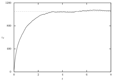
Figure 1: Charging of dust particles in a dusty plasma.

II.1 Sheath equations and sheath structure

Consider now a plasma sheath in steady state. Far away from the sheath, the plasma potential vanishes and other plasma parameters approaches their bulk (equilibrium) values i.e. $x\to\infty$, $\phi\to 0$, $u_{i}\to u_{0}\equiv M$, $p_{i}\to 1$, $n_{i}\to 1$, $z_{d}=z_{d}/z_{d0}\to 1$. $M$ is the Mach number which is the ratio of the ion velocity far away from the sheath to that of ion-sound velocity. For a stationary sheath, the steady state equations are,

$$\frac{\partial}{\partial x}(n_{i}u_{i}) = 0,$$ (19)

$$u_{i}\frac{\partial u_{i}}{\partial x}+\gamma\sigma n_{i}^{\gamma-2}\frac{\partial n_{i}}{\partial x} = -\frac{\partial\phi}{\partial x},$$ (20)

$$u_{i}\frac{\partial\varphi_{d}}{\partial x} = f(n_{i},\phi,\varphi_{d}).$$ (21)

From the continuity equation, we have

$$n_{i}=M/u_{i}.$$ (22)

Integration of Eq.(20) thus results the conservation of total energy flux which is a combination of the kinetic flux, enthalpy flux, and electrostatic flux,

$$\phi=\frac{1}{2n_{i}^{2}}M^{2}\left(n_{i}^{2}-1\right)+\frac{\gamma\sigma}{(\gamma-1)}\left(1-n_{i}^{\gamma-1}\right).$$ (23)

An expression for $n_{i}$ as a function of $\phi$ can be found from Eqs.(20,22), $n_{i}={\cal F}(\phi)$. For arbitrary $\gamma$, the above equation has to be solved numetically. For $\gamma=3$ however, we can find an analytical expression for $n_{i}(\phi)$ as,

$$n_{i}=\frac{1}{2\sqrt{3\sigma}}\left[\left\{\left(M+\sqrt{3\sigma}\right)^{2}-2\phi\right\}^{1/2}-\left\{\left(M-\sqrt{3\sigma}\right)^{2}-2\phi\right\}^{1/2}\right].$$ (24)

The signs in front of the square roots are fixed through the boundary condition on $n_{i}$. As the ion density can be expressed as a function of the plasma potential, $n_{i}\equiv n_{i}(\phi)$, Poisson’s equation can be integrated to get,

$$\frac{1}{2}\left(\frac{d\phi}{dx}\right)^{2}+V(\phi,M,\sigma,\gamma)=0,$$ (25)

where $V(\phi,M,\sigma,\gamma)$ is the equivalent Sagdeev potential or pseudo potential for a sheath, given by,

$$V(\phi,\varphi_{d},M,\sigma,\gamma)=1-e^{\phi}+\delta_{i}\int_{0}^{\phi}n_{i}(\phi)\,d\phi-\delta_{d}\int_{0}^{\phi}z_{d}(\phi)\,d\phi.$$ (26)

For real solution, we must have

$$V(\phi,M,\sigma,\gamma)<0$$ (27)

for all values of $\phi$. We can also determine the minimum velocity for the ions ($u_{0}\equiv M$) at the sheath boundary (the Bohm condition) from this condition. The boundary condition on $V$ is: at $\phi=0$, $V(\phi)=0$.

A few noteworthy points are in order at this moment. If the dust-charge fluctuation is absent, it means the electron and ion currents to the dust particles always balance each other so that at all time, we have

$$f(n_{i},\phi,\varphi_{d})=0.$$ (28)

This equation can be numerically solved for $z_{d}$ (or for $\varphi_{d}$) as a functions of $\phi$ and the Sagdeev potential can be constructed numerically. However, in presence of dust-charge fluctuation, the problem has to be solved numerically. Multiplying Eq.(21) with $n_{i}$ and using Eq.(19), we can write

$$\frac{\partial}{\partial x}(n_{i}u_{i}\varphi_{d})=n_{i}f(n_{i},\phi,\varphi_{d}),$$ (29)

where we note that $M=n_{i}u_{i}$. Thus, using Poisson equation, Eq.(26), and the above equation, one can summarily construct the following numerical model

$$\frac{d^{2}\phi}{dx^{2}} = e^{\phi}-\delta_{i}n_{i}-\alpha\delta_{d}\varphi_{d},$$ (30)

$$\frac{d\varphi_{d}}{dx} = \frac{n_{i}}{M}f,$$ (31)

$$n_{i} = {\cal F}(\phi).$$ (32)

This problem is a coupled boundary and initial value problem involving a nonlinear Poisson equation, which needs to be solved with a hybrid approach. We have solved this model with a finite-difference algorithm with a Newton-iteration for the nonlinear Poisson equation with Dirichlet boundary conditions. During every Newton iteration of the boundary value problem, we use a single, 4th order Runge-Kutta step for the initial value equation, Eq.(31). Of course, in every step, the nonlinear algebraic equation, Eq.(32) needs to be solved for $n_{i}$, which we have solved using a nonlinear solver. However, as we shall see, although the boundary values for the Poisson equation can be estimated quite accurately, the same can not be said for the initial value for Eq.(31). This has to be estimated iteratively following the negativity condition (27) for a numerically constructed Sagdeev potential.

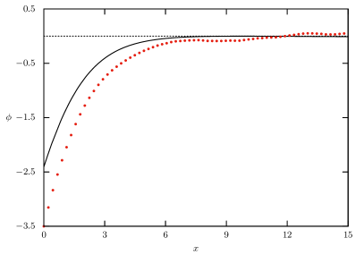
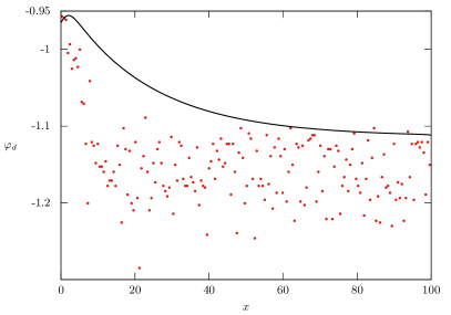
Figure 2: Plasma potential $\phi$ and dust potential $\varphi_{d}$ with dust-charge fluctuation.

The boundary values for the plasma potential can be estimated by considering the current at the wall and infinity. Far away from the sheath, the plasma potential must approach the bulk potential i.e. zero, $\phi_{x\to\infty}=0$. Assuming the current at the wall be zero, for a stationary sheath we have

$$j_{e}+j_{i}+j_{d}=0,$$ (33)

where $j_{e,i,d}$ are the electron, ion, and dust currents to the wall. However in view of inertia of the massive dust particles in comparison to the electrons and ions, it can be safely assumed that in the electron and ion timescale, the contribution to the wall current by the dust particles is negligibly small,

$$j_{e}+j_{i}\approx 0$$ (34)

for all practical purposes. The electrons, which reach the wall with a minimum velocity $v_{\textrm{min}}$ by overcoming the negative potential at the wall $\phi_{w}$, contribute to electron-current at the wall. So, we have

$$v_{\textrm{min}}=\left(-\frac{2e\phi_{w}}{m_{e}}\right)^{1/2},$$ (35)

so that we have for the electron current

$$j_{e}=-e\int_{v_{\textrm{min}}}^{\infty}\int_{-\infty}^{\infty}\int_{-\infty}^{\infty}vf_{e}(v)\,d\bm{v},$$ (36)

where $f_{e}(v)$ is the electron velocity distribution function. For a Maxwellian velocity distribution, we have the expression

$$j_{e}=-n_{e0}e\left(\frac{T_{e}}{2\pi m_{e}}\right)^{1/2}\exp\left(\frac{e\phi_{w}}{T_{e}}\right).$$ (37)

The ion current at the wall is given by

$$j_{i}=en_{i0}u_{i}\left(\frac{T_{e}}{m_{i}}\right)^{1/2}=en_{0}u_{0}\left(\frac{T_{e}}{m_{i}}\right)^{1/2},$$ (38)

where $u_{0}$ is the ion velocity (the Mach number) at the sheath boundary. From the neutrality condition (34), we can solve for the wall plasma potential (normalised) as

$$\phi_{w}=-2.84+\ln M.$$ (39)

As the plasma potential vanishes far away from the sheath, we can determine the dust potential as well, from the charging equation as at $\infty$, $\partial\varphi_{d}/\partial x\to 0$, so that $f(\varphi_{d})|_{x\to\infty}=0$. This determines the $\varphi_{d}|_{x\to\infty}=\varphi_{d\infty}$ as

$$\varphi_{d\infty}=\sigma-W(z),$$ (40)

where $W(z)$ is the Lambert $W$ function with

$$z=\frac{\sigma^{1/2}}{\delta_{i}\delta_{m}n_{i}}e^{\sigma}.$$ (41)

Numerically however it is not possible to use this value as an initial value for solving the dust-charging equation as we need to start at very large distance from the wall. We realize that although the dust current at the wall is negligible, the dust potential $\varphi_{dw}$ at the wall need not be so and is expected to be small negative. So, we continue solving the whole model starting with $\varphi_{dw}=0$ iteratively with the condition that the Sagdeev potential $V(\phi,\varphi_{d},M,\sigma,\gamma)<0$ [22] in the entire sheath region for the defined parameters. The results of this calculation is shown in Fig.2 where we plot the plasma potential $\phi$ and the dust potential $\varphi_{d}$ as we go away from the sheath to the bulk plasma. The solid lines in each panel indicate the theoretical curves obtained for $\gamma=5/3$ for $M=1.5$ and the dots indicate the equivalent results from the h-PIC-MCC simulation with parameters as mentioned before. We must note that in the simulation, there is no fixed Mach number for the ions as they enter the sheath with different Mach numbers starting with the minimum.

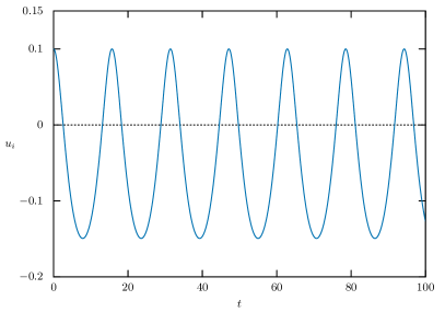
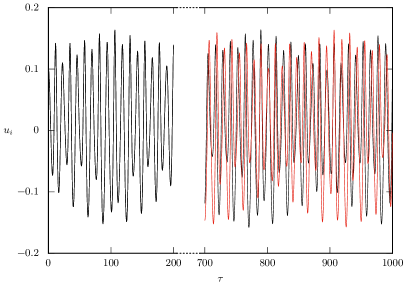
Figure 3: The periodic oscillations of the system represented by Eq.(49) in absence of dust-charge fluctuations (left). On the right, the same oscillations with driven dust-charge fluctuation is presented where the sensitivity to the initial conditions can be clearly seen. All plasma parameters are as in the case of h-PIC-MCC simulation.

III Driven dust-charge fluctuation and chaos

A dynamical model demonstrating chaos in dusty plasma driven by dust-charge fluctuation was formulated by Momeni et al. in 2007 [17, 23]. In that work, they reduced the dusty plasma dynamical model to a single second order, non-autonomous differential equation in dust density, which exhibits chaotic dynamics in the dust-acoustic regime. This single differential equation is described as a Van der Pol-Mathieu (VdPM) equation owing to its Van der Pol-like term and a Mathieu-like non-autonomous term

$$\frac{d^{2}n_{d}}{dt^{2}}-\left(\alpha-\beta n_{d}^{2}\right)\frac{dn_{d}}{dt}+\omega_{0}^{2}(1+h\,\cos\gamma t)n_{d}=0,$$ (42)

where $n_{d}$ is the dust density, $\omega_{0}\sim\omega_{pd}$ the characteristic oscillation frequency of the system of the order of dust-plasma frequency $\omega_{pd}$. The non-autonomous term results from the time-dependent dust-charge fluctuation term, represented by $h\cos\gamma t$, with $h$ as the amplitude of the fluctuation and $\gamma$ as the fluctuation frequency. As seen from the equation, the dust-charge fluctuation term is supposed to oscillate harmonically. The authors assumed that the dust particles are continuously created and destroyed through a source term $\alpha n_{d}$ and a loss term $\beta n_{d}^{3}/3$ in the 1-D dust continuity equation [17]

$$\frac{\partial n_{d}}{\partial t}+\frac{\partial}{\partial x}(n_{d}u_{d})=\alpha n_{d}-\frac{1}{3}\beta n_{d}^{3},$$ (43)

where the source terms is assumed to appear due to the production of charged dust grains through electron absorption and the loss terms is due to a three-body recombination term.

It is important to realize that in the above work, though the authors do not describe why the time-dependent dust-charge fluctuation term is harmonic, it can be argued to be originating from an externally driven source – such as photoemission, which is what we are investigating in this work. In this work, we provide a prescription where chaotic oscillations are experimentally realizable. Our parameters are however in the ion-acoustic regime unlike the above model. In what follows, we construct a model which can demonstrate chaotic ion dynamics through driven dust-charge fluctuation. There is however an important difference between the above mentioned work and ours is that here we are using the dust-charge fluctuation as a mechanism to drive the chaotic dynamics in ion velocity whereas in the former the same mechanism is to drive the dynamics is dust density.

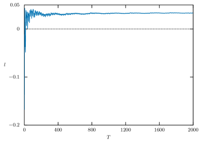
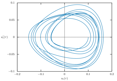
Figure 4: The maximal Lyapunov exponent $l$ of the system (left) shown for the first $\tau\sim 500$ and the phase portrait in the chaotic regime (right). The value of $l\sim 0.033$.

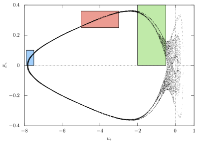
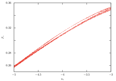
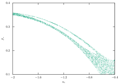
Figure 5: Poincaré plots for the system in the chaotic regime. Subsequent panels are zoomed out plots of the corresponding regions shown in the first plot.

III.1 A chaotic ion-dynamics model

We now construct a ion-dynamical model from Eqs.(6-9) for the driven dust-charge case, which can exhibit chaos. We introduce a scaled time $\tau=t-x/v_{0}$ so that the equations can be converted to a single variable. In terms of the scaled variable, we have $\partial/\partial t\equiv\partial/\partial\tau$ and $\partial/\partial x\equiv-v_{0}^{-1}\partial/\partial\tau$. So, Eqs.(6,7,9) become

$$\frac{\partial n_{i}}{\partial\tau}-\frac{1}{v_{0}}\frac{\partial}{\partial\tau}(n_{i}u_{i}) = 0,$$ (44)

$$\frac{\partial u_{i}}{\partial\tau}-\frac{u_{i}}{v_{0}}\frac{\partial u_{i}}{\partial\tau}-2\frac{\sigma}{v_{0}}\frac{\partial n_{i}}{\partial\tau} = \frac{1}{v_{0}}\frac{\partial\phi}{\partial\tau},$$ (45)

$$\frac{1}{v_{0}^{2}}\frac{\partial^{2}\phi}{\partial\tau^{2}} = n_{e}-\delta_{i}n_{i}+\delta_{d}z_{d}(\tau),$$ (46)

where for simplicity we assumed $\gamma=2$. Eq.(44) can be integrated to obtain the ion density

$$n_{i}=\frac{v_{0}-u_{0}}{v_{0}-u_{i}},$$ (47)

where we have assumed that at infinity $u_{i}(\tau)\to u_{0}$ and $n_{i}(\tau)\to n_{i0}\equiv 1$ (note the normalization). Similarly Eq.(45) can be integrated to obtain the plasma potential

$$\phi=\frac{1}{2}\left(u_{0}^{2}-u_{i}^{2}\right)-v_{0}(u_{0}-u_{i})+2\sigma\left(1-\frac{v_{0}-u_{0}}{v_{0}-u_{i}}\right),$$ (48)

where we have imposed the condition that at infinity (bulk plasma), $\phi(\tau)\to 0$. Using the Poisson equation and the above expressions, we finally arrive at a coupled 2-D nonlinear differential equation in $u_{i}$

$$u_{i}^{\prime\prime}A+u_{i}^{\prime 2}B+C=0,$$ (49)

where the ‘^′’ denotes $d/d\tau$ and

$$A = \frac{1}{v_{0}^{2}}\left(\mu_{i}-2\sigma\frac{\mu_{0}}{\mu_{i}^{2}}\right),$$ (50)

$$B = -\frac{1}{v_{0}^{2}}\left(1+4\sigma\frac{\mu_{0}}{\mu_{i}^{3}}\right),$$ (51)

$$C = \delta_{i}\frac{\mu_{0}}{\mu_{i}}-e^{\phi}-\delta_{d}z_{d}(\tau),$$ (52)

with $\mu_{0}=v_{0}-u_{0}$ and $\mu_{i}=v_{0}-u_{i}$. With an autonomous term involving the time-varying dust-charge $z_{d}(\tau)$, Eq.(49) fulfills all the basic characteristics which are necessary for exhibition of chaotic dynamics. The driven dust-charge term $z_{d}(\tau)$ can be designed as

$$z_{d}(\tau)=\varrho\,\cos(\nu t)^{\Delta},\quad(\Delta\in{\rm integer}),$$ (53)

where $\varrho$ is the amplitude and $\nu$ is the frequency of the driven dust-charge fluctuation. It can be numerically shown that in absence of any dust-charge fluctuation i.e. when $z_{d}\equiv 1$, for $v_{0}>u_{0}$, Eq.(49) admits periodic solutions (See Fig.3).

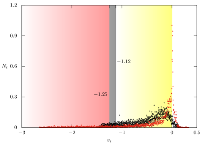
Figure 6: The ion velocity distributions in the sheath region (up to about $x\apprle 10\lambda_{D}$) with and without dust-charge fluctuation. While the black points indicate the distribution with constant dust-charge, the red points indicate the same with dust-charge fluctuation. Please see the accompanying text for explanation about the different regions indicated in the figure. The sheath is on the left $(x=0)$ and the ‘$-$’ sign indicates left-moving ions going toward the sheath.

III.1.1 $v_{0}\gg u_{0}$

We now explore the regime $v_{0}\gg u_{0}$ in presence of driven dust-charge fluctuation. Our parameters are $\varrho\sim 0.1$, which is a small positive quantity and $\nu\sim 0.4$. We take $u_{0}\sim 10^{-4}$ and $v_{0}\sim 1$. The parameter $\Delta$ is set to $2$. Note that when $v_{0}\gg u_{0}$, it is as if $\tau\sim t$ and the variables are almost constant in space. This points out to a localised disturbance where chaotic oscillation might be observed. The rest of the plasma parameters are as in case of the simulation.

The results of this analysis is presented in Fig.3 and 4. The left panel of Fig.3, shows the periodic oscillations when $z_{d}=1$ or equivalently when $\varrho=0$ i.e. no dust-charge fluctuation. The right panel shows the same oscillations (in black and red colors) when $\varrho=0.1$ (the other parameters are as mentioned before). One can clearly see the sensitivity of the oscillations where both of these differ by a factor $\sim 10^{-5}$ in the initial conditions. We carry out a Lyapunov exponent calculation [24] on Eq.(49) for these oscillations and the results are presented in Fig.4, where the left panel shows the maximal Lyapunov exponent of the system $l\sim 0.033$, which is positive signifying chaos and in the right panel, the phase portrait of the system is shown. In calculating the Lyapunov exponent, we have evolved the system for $\tau\simeq 2000$ with a step-size of $0.01$, gathering about $2\times 10^{5}$ points. The corresponding Poincaré plots [24] are shown in Fig.5, which shows the typical characteristics of a fractal construction, signifying chaos.

IV hybrid-PIC-MCC simulation of dusty plasma

Our simulation model comprises of a 1-D electrostatic particle-in-cell (PIC) code with the capabilities of having various boundary conditions including periodic boundary [8, 9, 10]. We note that the usual PIC model does not have any collisional transfer of momenta. Also the particles in a PIC model are macro-particles comprising of a number of real-life particles. As such, any collision implemented under the PIC formalism will actually account for collisions en masse. However, in a limited way, collisions can be implemented in a PIC formalism through PIC-Monte Carlo Collision (PIC-MCC) algorithm. It consists of using a randomized probability to account for the collisions based on the theoretical estimation of the collision cross sections. Multistep Monte Carlo Collision is also another way of including collisions [25]. We rather use a hybrid method to estimate the collisions of dust particles with electrons and ions, which is described as the hybrid-PIC-MCC (h-PIC-MCC) method [9, 10]. The details of this algorithm and the code is described in two papers by Changmai and Bora [8, 9].

IV.1 Dust-charge fluctuation and plasma sheath

In order to account for the dust charge fluctuation in our simulation, we assume that whenever a collision of the dust particle with an electron occurs, it contributes to an increase of negative charge on the surface of the dust particle [9, 10]. This is effected by decreasing the number of electrons in the simulation domain accompanied by an equivalent increase of electron dust charge number $z_{d}$. The accumulation of positive charge on the surface of a dust particle is, however, modeled by assuming that whenever an ion-collision occurs, an electron is ejected from the dust particle which causes $z_{d}$ to decrease (equivalently charging the dust particle positively) and an increase of a plasma electron in the simulation box. Hence, the total ion number in the simulation domain remains constant while the total electron number and dust charge fluctuate depending on the type of collisions. Without loss of any generality, this process can be extended up to any number of dust particles, thereby simulating an environment of a dusty plasma.

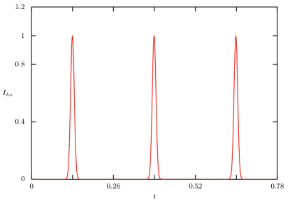
Figure 7: The periodic burst of photoemission.

In our simulation, we however assume that the dust particles are cold and stationary, which is consistent with the characteristic time scale of the simulation i.e. ion-acoustic time scale and is also what we consider in the theoretical buildup. We also introduce a randomized probability $p_{i,e}$, which determines whether a charged particle is absorbed by a dust particle in the event of a collision, hence the name h-PIC-MCC. At this point, it should be noted that every binary collision in this formalism is actually a collision between two macro-particles, which in reality, does not happen. Nevertheless, in the ion acoustic time scale, this procedure is able to capture the essential physics involving dust-ion-acoustic (DIA) dynamics. For all practical purposes, the dust particles act as collections of electrons, assuming that the dust particles charge to a net negative potential as the plasma attains its equilibrium. Our prescription for dust charging conserves the plasma quasi-neutrality condition

$$n_{i}=n_{e}+z_{d}n_{d}.$$ (54)

The dust macro-particles are uniformly distributed in the domain with zero net charge. The dust radius is fixed at $r_{d}\sim 10^{-2}\lambda_{{\rm D}e}$. As mentioned before, in Fig.1, the average charging of single dust particle is shown, calculated from the total count of electron depletion in the simulation domain. As can be seen from the figure, on average, a single dust particle attains an equilibrium net charge of about $Q_{d}\sim-500e$. The equivalent dust number density can be calculated from the quasi-neutrality condition as $n_{d}\sim 4.2\times 10^{12}\,{\rm m}^{-3}$.

We now present the results of our h-PIC-MCC simulation on the effect of dust-charge fluctuation. We note that the Bohm criterion for a plasma sheath with cold ion and constant dust-charge is $M>M_{c}=\sqrt{\delta_{i}}$, which gets modified for dust-charge fluctuation [6]

$$M_{c}^{2}=\frac{-\delta_{i}+2q_{d0}+\sqrt{(3\delta_{i}-2q_{d0})^{2}+8(\delta_{i}-1)[2-(3\delta_{i}-2)/q_{d0}]}}{2[1-(\delta_{i}-1)/q_{d0}]},$$ (55)

where $q_{d0}$ is the normalised dust-charge at the sheath edge. For the plasma parameters as mentioned in the previous paragraph, $M_{c}\simeq 1.12$ for constant dust-charge and gets modified to $M_{c}\simeq 1.25$ in presence of dust-charge fluctuation. In Fig.6, we show the ion velocity distribution in the sheath region. Note that the sheath region extends only up to about $\sim 10\lambda_{D}$ (see the first panel in Fig.2). In Fig.6, we show the distributions for dust particles with constant charge (black dots) and with charge fluctuation (red dots). As expected, the penetrating velocity of the ions into the sheath increases in presence of dust-charge fluctuation. Different regions indicated in the figure represent the pre-sheath region, sheath-edge for constant dust-charge, and sheath-edge with dust-charge fluctuation. The respective sheath-edges are defined through the values $M=M_{c}$ and the pre-sheath region is defined when the ion velocity is just zero demarcating the let and right-moving ions. So, in this case, we define the pre-sheath region is where ions have just started to move toward the left i.e. toward the sheath. The number of ions in the figure is normalised by its maximum value.

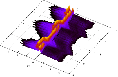
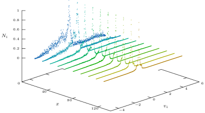
Figure 8: The evolution of the plasma sheath in time (first panel) and in space (second panel) in terms of ion velocity distribution. In the first panel, the ion velocity distribution is plotted in the near-sheath region in time, where the oscillation of the sheath (in terms of periodic peaking of ion velocity) can be clearly seen. In the second panel, the ion velocity distribution function is plotted as one moves away from the sheath (the wall is at $x=0$).

IV.2 Driven dust-charge fluctuation – Chaotic ion dynamics

We now consider the case for driven dust-charge fluctuation, where we drive the dust-charge fluctuation through a controlled emission of photoelectrons from the sheath-side wall by periodically exposing the wall to strong UV radiation. The periodic emission of photoelectrons can be mathematically represented (in the photoemission current to the dust particles) as

$$I_{h\nu}=\varrho\,\cos(\nu t)^{2\Delta},\,\Delta\gg 1\,({\rm integer}),$$ (56)

where $\nu$ is the periodicity of the photoemission burst (see Fig.7) and $\varrho$ is its amplitude. In our case, $\nu^{-1}\sim 0.02t$, time being normalised by $\omega_{pi}^{-1}$. Eq.(56) is same as Eq.(53), except that it is now in the photoemission current to the dust particles which has the same role in our simulation scenario as Eq.(53) in the theoretical formalism.

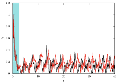
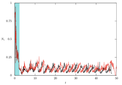
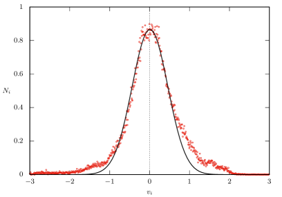
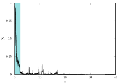
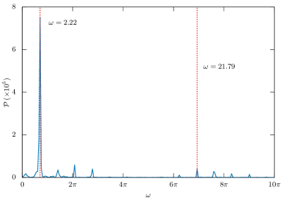
Figure 9: First row: Two snapshots of the ion velocity distribution in the sheath and the near-sheath region for two different dust densities. The first panel is for $n_{d}\sim 4.2\times 10^{12}\,{\rm m}^{-3}$ and the second one is for $n_{d}\sim 1.5\times 10^{12}\,{\rm m}^{-3}$. Both the plots show the characteristics signature of chaotic dynamics as confirmed by our chaos analysis. The shaded regions in both the plots indicate initial transient regions as the distributions evolve in time. The change in oscillation patterns in the both the plots corresponds to a change of $\sim 10^{-4}$ in the burst duration of the emission of photoelectrons while the periodicity of the bursts are same in all the cases.
 
Second row: The ion distribution function in the sheath region and in the bulk plasma.
 
Third row: The ion distribution function in presence of periodic photoemission bursts as in the first cases but without any dust-charge fluctuation. The distribution is purely stochastic (left). The right panel shows the power spectral density ${\cal P}$ of these oscillations shown in the left panel of the first row of this figure.

As we have periodic photoelectron bursts from the sheath-side wall, the plasma sheath oscillates between a classical sheath and an inverse sheath. This oscillation can be clearly seen from the reconstruction plots of the ion velocity distribution as shown in Fig.8. The first panel of the plots shows the time evolution of the ion distribution function in the near-sheath region, while the second panel shows the evolution of the sheath as one moves away from the wall. We can clearly see the periodic formation of ion-velocity peaks in the first panel. In the second panel, we can see that the ion velocity distribution gradually approaches a Maxwellian distribution as one goes away from the wall. In Fig.9, we show the chaotic evolution of the ion velocity distribution in the sheath and the near-sheath region. It should however be noted that in presence of the driven photoemission, there is no clear sheath boundary as the sheath itself oscillates in time. We show the power spectral density ${\cal P}$ of these oscillations (first panel, first row of Fig.9) in the second panel of the third row of Fig.9. The spectral density shows a dominant peak at frequency $\sim 0.354$ corresponding an angular frequency of $\omega\sim 2.22$, which is the large-scale oscillations that we see. The second dominant peak in ${\cal P}$ away from the large-scale oscillations is at a frequency $\sim 3.47$ corresponding an angular frequency of $\omega\sim 2.22$ which represents the fine-scale oscillations. These fine-scale oscillations actually correspond to the frequency of the driven photoemission bursts frequency shown in Fig.7, represented by Eq.(56). So, what we see is that the periodic bursts of photoemission of electrons are exciting a very low frequency large-scale oscillations in ione velocity through dust-charge fluctuations.

Figure 10: An estimate of the dominant Lyapunov exponent as determined through Wolf’s algorithm (right axis) and the $K$ values from the 0-1 test (left axis) for the two sampled data shown in the first row of Fig.9.

We initially perform two different tests for chaos on the ion velocity distributions – (a) estimation of the dominant Lyapunov exponent $l$ from a time series with the help of Wolf’s algorithm [26] and (b) perform 0-1 test for chaos. While Wolf’s method calculates the dominant Lyapunov exponent through reconstruction of the phase space (also referred to as delay reconstruction) from the time series data and detection of orbital divergence, the 0-1 test estimates the growth rate of divergence from the time-averaged mean square displacement of the time series data. We use Wolf’s algorithm as provided by the authors through their very well-developed Matlab / Octave interface. In case of the 0-1 test, we use a very recent work involving Chaos Decision Tree Algorithm by Toker et al. [27] to rule out stochasticity and random noise. Briefly, in 0-1 test, two 2-D system $p(n)$ and $q(n)$ are derived from the 1-D time series data $v(n)$ for $n=1,2,\dots$

$$p(n+1) = p(n)+v(n)\,\cos(cn),$$ (57)

$$q(n+1) = q(n)+v(n)\,\sin(cn),$$ (58)

where $c\in[0,2\pi]$ is random. For a particular $c$, the solution to Eqs.(57,58) requires

$$p_{c}(n) = \sum_{j=1}^{n}v(j)\,\cos(jc),$$ (59)

$$q_{c}(n) = \sum_{j=1}^{n}v(j)\,\sin(jc).$$ (60)

It can be shown that if $v(n)$ are regular, $p,q$ are bounded, while they display asymptotic Brownian motion if $v(n)$ are chaotic. The time-averaged mean squared displacement of $p,q$ is then calculated as

$${\cal M}_{c}(n)=\frac{1}{N}\sum_{j=1}^{N}\left([p_{c}(j+n)-p_{c}(j)]^{2}+[q_{c}(j+n)-q_{c}(j)]^{2}\right)+\sigma\eta_{n},$$ (61)

where $\eta_{n}\in[-1/2,+1/2]$ is a uniform random deviate and $\sigma$ is the noise level for a total of $N$ number of sampled data in the time series. Finally the growth rate $K$ is calculated as

$$K=\lim_{n\to\infty}\frac{\log{\cal M}_{c}(n)}{\log n}.$$ (62)

For chaotic data the median $K\to 1$ and for periodic system $K\to 0$.

In Fig.10, we show the determined values of $l$ and $K$ from these two tests and as can be seen, both tests points to the fact that the sampled data are indeed chaotic in nature.

IV.2.1 Recurrence plots

As a final test, we construct the recurrence plots [28, 29] for the oscillations shown in Fig.9. The purpose of a recurrence plot is to visualize the recurrences of a dynamical system. It is a very powerful tool which enables us to construct complex dynamical pattern from a single time series. In summary, a recurrence plot is based on the following recurrence relation [29]

$$\bm{R}_{ij}=\begin{cases}1:&\vec{x}_{i}\approx\vec{x}_{j},\\ 0:&\vec{x}_{i}\not\approx\vec{x}_{j}\end{cases}\quad i,j=1,2,\dots,N,$$ (63)

where the $\left\{\vec{x}_{i}\right\}_{i=1}^{N}$ is a system in its phase space and $N$ is the number of considered states. Essentially $\bm{R}_{i,j}$ is a Heaviside function which depends on a threshold condition $\varepsilon$ which determines whether $\vec{x}_{i}\approx\vec{x}_{j}$. If we assume that the state of a dynamical system $\vec{x}(t)$ is specified by $d$ components, we can a form vector with these components [29]

$$\vec{x}(t)=(x_{i}(t))^{T},\quad i=1,2,\dots,d$$ (64)

in the $d$-dimensional phase space. In a purely mathematically constructible setup, all these components are known and one can easily construct the phase space. However, in experiments and in a simulation like ours, we have only one time series with only one observable, which in this case is the ion velocity. So, we have one discrete time series

$$u_{i},\quad i=1,2,\dots,N,$$ (65)

with $\Delta t$ as the sampling interval on the basis of which we have to reconstruct the phase space with the help of a time delay, as mentioned before [29]

$$\vec{x}_{i}=\sum_{j=1}^{m}u_{i+(j-1)\tau}\vec{e}_{j},\quad\vec{e}_{i}\cdot\vec{e}_{j}=\delta_{ij},$$ (66)

where $m$ is the embedding dimension, $\tau$ is the time delay, and $\vec{e}_{j}$ are the unit vectors which span an orthogonal system. For $m\geqslant 2D_{2}+1$, where $D_{2}$ is the correlation dimension of the underlying attractor, with the help of Taken’s theorem one can show the existence of a diffeomorphism between the original and the reconstructed phase space or simply speaking, one can use the reconstructed attractor to study the original one but in a different coordinate system. So, our recurrence plot is then defined by the relation

$$\bm{R}_{ij}(\varepsilon)=H\left(\varepsilon-\left\|\vec{x}_{i}-\vec{x}_{j}\right\|\right),\quad i,j=1,2,\dots,N,$$ (67)

where $N$ is the number of measured points , $H(x)$ is the Heaviside step function, and $\left\|\cdot\right\|$ denotes norm. In our case, we have used an Euclidean $L_{2}$ norm.

In Fig.11, we have shown 6 recurrence plots for the chaotic oscillations shown in Fig.9. The embedding dimension is chosen to be $4$ and the delay used is $5$. The threshold is used about $\sim 8.9\%$ of the maximum amplitude of the oscillations. Clockwise from the top in the figure, we have used a sampling interval $t_{{\rm smaple}}=2,10,50,100$ respectively over a total of $32500$ time steps $\Delta t$. We can see that as the sampling interval increases, the plots increasingly reveal the signature of a chaotic oscillation, signifying the small fine-scale periodic oscillations in the first plot with geometric recurrences when the sampling interval is small (the first plot in the first row) and a fractal pattern in the last of these four plots (the second plot in the second row). The first plot in the third row is similar to the second plot of the second row except that we have superimposed the corresponding plot with a map having no threshold (all recurrences). The last plot in the figure represents the one for ion velocity distribution time series with constant dust charge, corresponding to the last plot of Fig.9. As one can see that this plot is similar to the one with random dynamics similar to Brownian motion signifying stochastic behaviour [29].

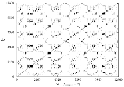
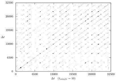
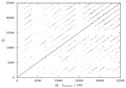
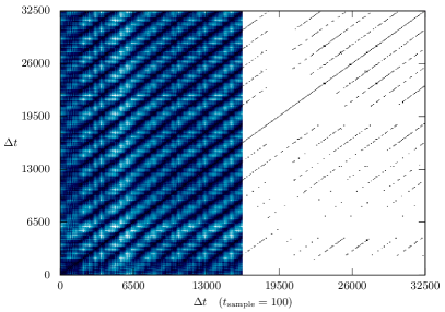
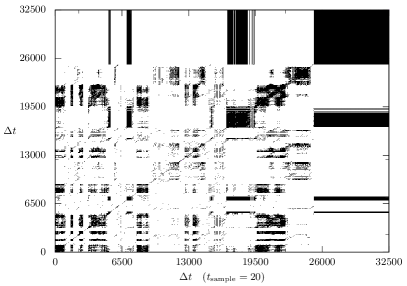
Figure 11: First & second rows: Recurrence plots for the chaotic oscillation shown in Fig.9 for different sampling intervals.
 
Third row: Same as the second plot of the second row, superimposed with a map with no threshold, displaying all recurrences (left) and a plot for a non-chaotic oscillation with constant dust-charge, displaying the signature for Brownian motion-like pattern.

V Conclusion

To summarise, in this work in brief, we consider a plasma model where electrons and ions are both thermal particles having cold and stationary dust grains with constant dust density. The time scale of our interest is ion-acoustic time scale. We develop the sheath equations and solve them numerically with a hybrid approach coupling the initial value problem of dust-charging equation with the boundary value problem of nonlinear Poisson equation. The whole theoretical formalism has been also replicated using a hybrid-PIC-MCC simulation and the theoretical results are found to be in good agreement with the simulation results.

Next, we consider that case for driven dust-charge fluctuation, which is the primary focus of this work. We use the plasma sheath as a candidate to induce a periodic dust-charge fluctuation through photoemission. The photoemission occurs when the sheath-side wall is exposed to UV radiation. So, by externally exposing the wall to UV radiation, the dust-charge fluctuation can be driven at an external frequency. Here, in the ion-acoustic regime, we focus on the ion dynamics in the sheath and the pre-sheath regions. We show that the relatively high frequency, of the order of about $\sim 3.5\omega_{pi}$, bursts of photoemission of electrons from the plasma sheath excite a chaotic super-harmonic large low-frequency wave in ion velocity through dust-charge fluctuation, which is confined to the sheath and the pre-sheath regions. With the help of appropriate analysis, we have established that the oscillations are indeed chaotic which owes its existence to the harmonic variation of the dust-charge fluctuation. The oscillations remains stochastic for constant dust-charge showing the in absence of sut-charge fluctuation, the sheath oscillations can not effectively propagate to the plasma.

References

- [1] S. Basnet, R. R. Pokhrel, and R. Khanal, IEEE Trans. Plasma Sci. 49, 1268 (2021).
- [2] G. C. Das, R. Deka, and M. P. Bora, Phys. Plasmas 23, 042308 (2016).
- [3] H. Mehdipour, I. Denysenko, and K. Ostrikov, Phys. Plasmas 17, 123708 (2010).
- [4] B. P. Pandey and A. Dutta, Pramana - J. Phys. 65, 117 (2005).
- [5] M. R. Jana, A. Sen, and P. K. Kaw, Physical Review E 48, 3930 (1993).
- [6] P. K. Shukla and A. A. Mamun, Introduction to Dusty Plasma Physics, Institute of Physics, Bristol and Philadelphia, 2002.
- [7] P. K. Shukla and V. P. Silin, Physica Scr. 45, 508 (1992).
- [8] S. Changmai and M. P. Bora, Phys. Plasmas 26, 042113 (2019).
- [9] S. Changmai and M. P. Bora, Sci. Rep. 10, 20980 (2020).
- [10] S. Changmai, Particle in cell (PIC) simulation of plasma sheath and related phenomena, PhD thesis, Gauhati University, Guwahati 781014, India (http://hdl.handle.net/10603/393033), 2022.
- [11] A. Piel, F. Greiner, T. Klinger, N. Krahnstöver, and T. Mausbach, Phys. Scr. T84, 128 (2000).
- [12] M. Megalingam, A. Sangem, and B. Sarma, Contrib. Plasma Phys. 60, e201900189 (2020).
- [13] B. Buti, Pramana - J. Phys. 49, 93 (1997).
- [14] C. S. Kuney and P. J. Morrison, Phys. Plasmas 2, 1926 (1995).
- [15] D.-G. Dimitriu and M. Agop, Handbook of Applications of Chaos Theory, chapter IV, pages 321–424, CRC Press, 2016.
- [16] R. K. Varma, P. K. Shukla, and V. Krishan, Physical Review E 47, 3612 (1993).
- [17] M. Momeni, I. Kourakis, M. Moslehi-Fard, and P. K. Shukla, J. Phys. A: Math. Theor. 40, F473 (2007).
- [18] A. Sen, S. Tiwari, S. Mishra, Predhiman, and Kaw, Adv. Space Res. 56, 429 (2015).
- [19] F. Cichocki, M. Merino, and E. Ahedo, Acta Astronaut. 146, 216 (2018).
- [20] R. Deka and M. P. Bora, Phys. Plasmas 27, 043701 (2020).
- [21] R. Deka and M. P. Bora, Phys. Plasmas 25, 103704 (2018).
- [22] R. Z. Sagdeev, in Reviews of Plasma Physics, edited by M. A. Leontovich, volume 4, page 23, Consultants Bureau, New York, 1966.
- [23] M. P. Bora and D. Sarmah, arXiv:0708.0684v1 (2007).
- [24] S. H. Strogatz, Nonlinear dynamics and chaos: with applications to physics, biology, chemistry, and engineering, CRC Press, 2018.
- [25] N. A. Gatsonis, R. E. Erlandson, and Meng, C.-I., Journal of Geophysical Research 99, 8479 (1994).
- [26] A. Wolf, J. B. Swift, H. L. Swinney, and J. A. Vastano, Phys. D: Nonlinear Phenom. 16, 285 (1985).
- [27] D. Toker, F. T. Sommer, and M. D’Esposito, Commun. Biol. 3, 11 (2020).
- [28] J.-P. Eckmann, S. O. Kamphorst, and D. Ruelle, Europhys. Lett. 4, 973 (1987).
- [29] N. Marwan, M. C. Romano, M. Thiel, and J. Kurths, Phys. Rep. 438, 237 (2007).