Data Imputation with Iterative Graph Reconstruction

Abstract

Effective data imputation demands rich latent “structure” discovery capabilities from “plain” tabular data. Recent advances in graph neural networks-based data imputation solutions show their structure learning potentials by translating tabular data as bipartite graphs. However, due to a lack of relations between samples, they treat all samples equally which is against one important observation: “similar sample should give more information about missing values.” This paper presents a novel Iterative graph Generation and Reconstruction framework for Missing data imputation(IGRM). Instead of treating all samples equally, we introduce the concept: “friend networks” to represent different relations among samples. To generate an accurate friend network with missing data, an end-to-end friend network reconstruction solution is designed to allow for continuous friend network optimization during imputation learning. The representation of the optimized friend network, in turn, is used to further optimize the data imputation process with differentiated message passing. Experiment results on eight benchmark datasets show that IGRM yields 39.13% lower mean absolute error compared with nine baselines and 9.04% lower than the second-best.

Introduction

Due to diverse reasons, missing data becomes a ubiquitous problem in many real-life data. The missing data can introduce a substantial amount of bias and make most machine learning methods designed for complete data inapplicable (Bertsimas, Pawlowski, and Zhuo 2017). Missing data has been tackled by direct deletion or by data imputation. Deletion-based methods discard incomplete samples and result in the loss of important information especially when the missing ratio is high (Luo et al. 2018). Data imputation is more plausible as it estimates missing data with plausible values based on some statistical or machine learning techniques (Lin and Tsai 2020) and allows downstream machine learning methods normal operation with the “completed” data (Muzellec et al. 2020).

Existing imputation methods discover latent relations in tabular data from different angles and normally with diverse assumptions. Simple statistical methods are feature-wise imputation, ignoring relations among features and might bias downstream tasks(Jäger, Allhorn, and Bießmann 2021). Machine learning methods such as k-nearest neighbors (Troyanskaya et al. 2001) and matrix completion (Hastie et al. 2015) can capture higher-order interactions between data from both sample and feature perspectives. However, they normally make strong assumptions about data distribution or missing data mechanisms and hardly generalize to unseen samples (You et al. 2020). Some solutions, e.g. MIRACLE (Kyono et al. 2021), try to discover causal relations between features which are only small parts of all possible relations. GINN (Spinelli, Scardapane, and Uncini 2020) discovers relations between samples while failing to model relations between samples and features. These methods typically fall short since they do not employ a data structure that can simultaneously capture the intricate relations in features, samples, and their combination.

A graph is a data structure that can describe relationships between entities. It can model complex relations between features and samples without restricting predefined heuristics. Several Graph Neural Networks(GNNs)-based approaches have been recently proposed for graph-based data imputation. Those approaches generally transform tabular data into a bipartite graph with samples and features viewed as two types of nodes and the observed feature values as edges (Berg, Kipf, and Welling 2017; You et al. 2020). However, due to a lack of sample relations, those solutions commonly treat all samples equally and only rely on different GNN algorithms to learn this pure bipartite graph. They fail to use one basic observation, “similar sample should give more information about missing values”. The observation, we argued, demands us to differentiate the importance of samples during the graph learning process.

Fig. 1 highlights the importance and difficulty in using the latent samples relations for data imputation. The tabular data with some missing data(Fig. 1a) can be easily transformed into a bipartite graph (Fig. 1b) and learned with GNNs solutions. However, if we know the ground-truth samples, we can form so-called friend networks by connecting similar samples with additional edges, shown in Fig. 1b. If we can fully exploit the friend network(by IGRM), the MAE of data imputation significantly drops, as shown in Fig. 1c. It clearly shows the importance of adopting the friend network. However, the large portion of missing data makes it hard to acquire accurate relations among samples. The cosine similarity on samples with missing data can be significantly biased, as shown in Fig. 1d, especially when the missing ratio is above 50%. Thus, a new mechanism is needed to learn accurate sample relations under a high missing ratio.

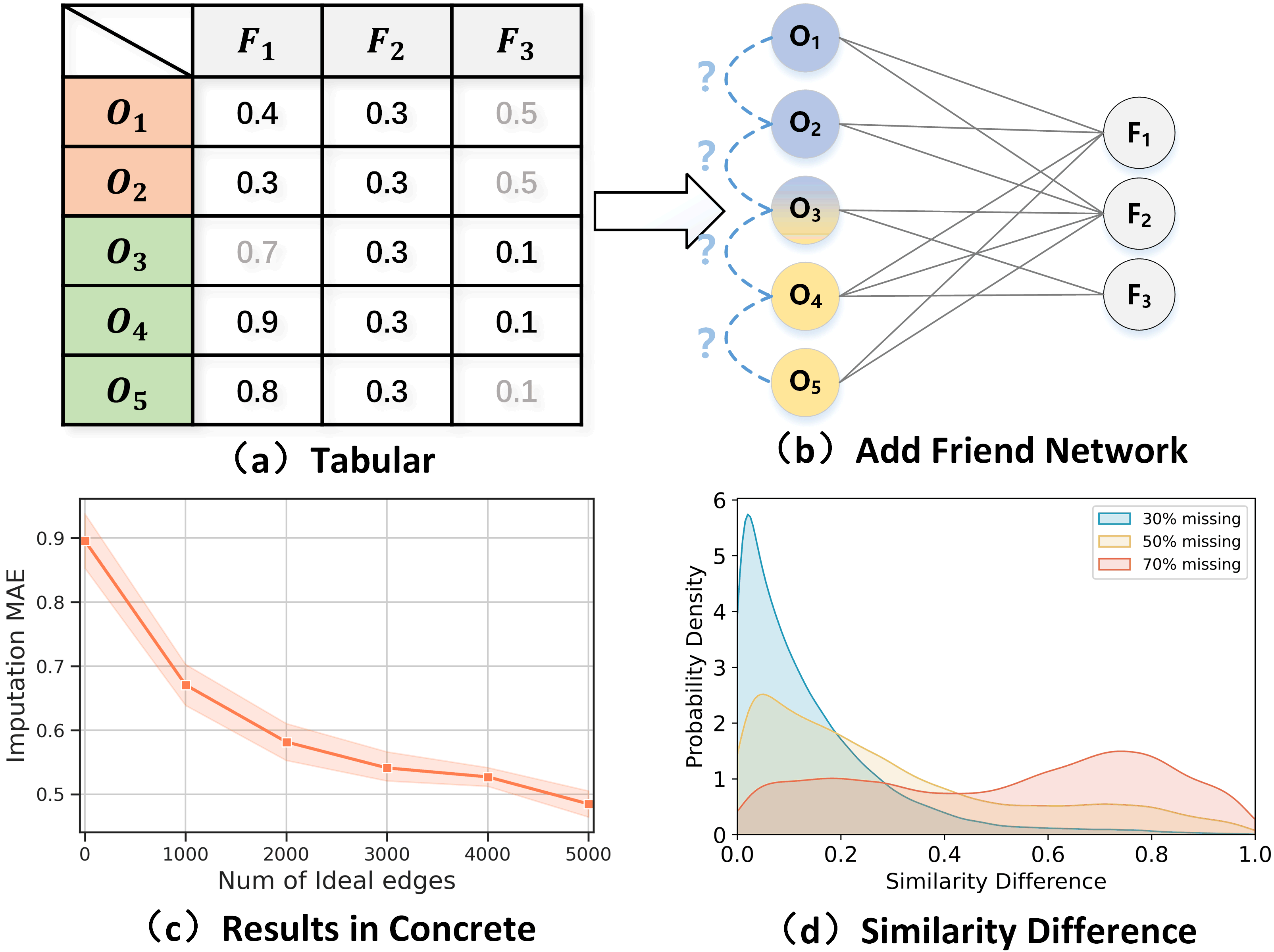
Figure 1: Imputation with friend network. Gray indicates missing values. Similar samples are marked with the same color with the ground-truth in a) and missing data in b). c) shows the trend of IGRM with adding an ideal friend network on Concrete in UCI dataset. d) shows similarity difference between ground-truth and data with missing.

This paper proposes IGRM, an end-to-end Iterative graph Generation and Reconstruction framework for Missing data imputation. IGRM goes beyond the bipartite graph with equal sample used in (You et al. 2020) by using the friend network to differentiate the bipartite graph learning process. IGRM also address the problem on how to generate an accurate friend network under a high missing ratio with an end-to-end optimization solution.

Contributions. 1) We propose a novel usage of “friend network” in data imputation. Introduction of the friend network augments traditional bipartite graphs with capabilities to differentiate sample relations. 2) To build an accurate friend network under missing data, IGRM is designed to be end-to-end trainable. The friend network is continuously optimized by the imputation task and is used to further optimize the bipartite graph learning process with differentiated message passing. 3) Instead of using plain attributes similarity, we innovatively propose the use of node embedding to reduce the impacts of a large portion of missing data and diverse distributions of different attributes. 4) We compared IGRM with nine state-of-the-art baselines on eight benchmark datasets from the UCI Repository (Asuncion and Newman 2007) and Kaggle. Compared with the second-best baselines, IGRM yields 9.04% lower mean absolute error (MAE) at the 30% data missing rate and even higher improvements in data with higher missing rates. A set of ablation studies also prove the effectiveness of our proposed designs.

Related Work

Studies on data imputation can be generally classified into statistics-based, machine-learning and deep-learning(including Graph) based imputations.

Statistics-based

include single imputations and multiple imputations. Single imputations are calculated only with the statistical information of non-missing values in that feature dimension (Little and Rubin 1987; Acuna and Rodriguez 2004; Donders et al. 2006), leading to possible distorted results due to biased sample distributions. Multivariate imputation by chained equations(MICE) (Buuren and Groothuis-Oudshoorn 2010; White, Royston, and Wood 2011; Azur et al. 2011) performs data imputation by combing multiple imputations. However, it still relies on the assumption of missing at random(MAR) (Little and Rubin 1987). Beyond the MAR assumption, MICE might result in biased predictions (Azur et al. 2011).

Machine and Deep-learning based

have been developed to address imputation, including k-nearest neighbors(KNN), matrix completion, deep generative techniques, optimal transport, and others. KNNs (Troyanskaya et al. 2001; Keerin, Kurutach, and Boongoen 2012; Malarvizhi and Thanamani 2012) are limited in making weighted averages of similar feature vectors, while matrix completions(Hastie et al. 2015; Genes et al. 2016; Fan, Zhang, and Udell 2020) are transductive and cannot generalize to unseen data. Deep generative techniques include denoising auto-encoders(DAE) (Vincent et al. 2008; Nazabal et al. 2020; Gondara and Wang 2017) and generative adversarial nets(GAN) (Yoon, Jordon, and Schaar 2018; Allen and Li 2016). They demand complete training datasets and may introduce bias by initializing missing values with default values. OT (Muzellec et al. 2020) assumes that two batches extracted randomly in the same dataset have the same distribution and uses the optimal transport distance as a training loss. Miracle (Kyono et al. 2021) encourages data imputation to be consistent with the causal structure of the data by iteratively correcting the shift in distribution. However, those approaches fail to exploit the potential complex structures in and/or between features and samples.

Graph-based.

Several graph-based solutions are proposed with state-of-art data imputation performances. Both GC-MC (Berg, Kipf, and Welling 2017) and IGMC (Zhang and Chen 2019) use the user-item bipartite graph to achieve matrix completion. However, they assign separate processing channels for each rating type and fail to generalize to the continuous data. To address this limitation, GRAPE (You et al. 2020) adopts an edge learnable GNN solution and can handle both continuous and discrete values. However, its pure bipartite graph solution largely ignores potentially important contributions from similar samples. GINN (Spinelli, Scardapane, and Uncini 2020) exploits the euclidean distance of observed data to generate a graph and then reconstruct the tabular by graph denoising auto-encoder.

Preliminaries

Let data matrix $\mathbf{D}\in\mathbf{R}^{n\times m}$ indicate the tabular with missing data, consisting of $n$ samples and $m$ features. Let $\mathbf{U}=\{u_{1},...,u_{n}\}$ and $\mathbf{V}=\{v_{1},...v_{m}\}$ be the sets of samples and features respectively. The $j$-th feature of the $i$-th samples is denoted as $\mathbf{D}_{ij}$. A binary mask matrix $\mathbf{N}\in\mathbf{\{}0,1\}^{n\times m}$ is given to indicate the location of missing values in tabular, where $\mathbf{D}_{ij}$ is missing only if $\mathbf{N}_{ij}=0$. In this paper, the goal of data imputation is to predict the missing data point $\hat{\mathbf{D}}_{ij}$ at $\mathbf{N}_{ij}=0$.

Definition 1. Data matrix as a bipartite graph. As illustrated in Fig. 1a-b, $\mathbf{D}$ can be formulated as a undirected bipartite graph $\mathbf{\mathcal{B}}=(\mathbf{U},\mathbf{V},\mathbf{E})$. $\mathbf{E}$ is the edge set where $\mathbf{E}_{ij}$ is an edge between $u_{i}$ and $v_{j}$: $\mathbf{E}=\{(u_{i},v_{j},{e}_{ij})|u_{i}\in\mathbf{U},v_{j}\in\mathbf{V},\mathbf{N}_{ij}=1\}$ where the weight of the edge equals the value of the $j^{th}$ feature of sample i, $e_{ij}$ = $\mathbf{D}_{ij}$. Here, nodes in $\mathbf{U},\mathbf{V}$ do not naturally come with features. Similar to the settings of GRAPE, let vector consist of vector 1 in $m$ dimension as $\mathbf{U}$ node features and $m$-dimensional one-hot vector as $\mathbf{V}$ node features.

Definition 2. Friend network. $\mathcal{F}=(\mathbf{U},\mathbf{A})$ represents similarity among the samples $\mathbf{U}$ by connecting similar samples denoted with a binary adjacency matrix $\mathbf{A}\in\{0,1\}^{n\times n}$. For any two samples $u_{i},u_{j}\in\mathbf{U}$, if they are similar, $\mathbf{A}_{ij}=1$. Here, let $\mathcal{N}(i)$ denotes function that returns the set of samples whom $u_{i}$ directly connects with in $\mathcal{F}$.

Definition 3. Cosine similarity with missing data. With the existence of missing values, the cosine similarity between two samples is defined as follows:

$$S_{ij}=cos(\mathbf{D}_{i:}\odot(\mathbf{N}_{i}\odot\mathbf{N}_{j}),\mathbf{D}_{j:}\odot(\mathbf{N}_{i}\odot\mathbf{N}_{j}))$$ (1)

where $\odot$ stands for the Hadamard product between vectors, $cos$ is the cosine similarity function. It computes pairwise similarity for all features, but only non-missing elements of both vectors are used for computations. As illustrated in Fig. 1d, this formulation might introduce a large bias since it is calculated on the subspace of non-missing features. When $\mathbf{N}_{i}\odot\mathbf{N}_{j}=\varnothing$, the calculated similarity would be NaN and is hard to be used for similarity evaluation.

Definition 4. Sample embedding-based similarity. The similarity of two samples $u_{i}$ and $u_{j}$ can be calculated with their embeddings $\mathbf{p}_{i}$ and $\mathbf{p}_{j}$:

$$S_{ij}^{{}^{\prime}}=cos(\mathbf{p}_{i},\mathbf{p}_{j})$$ (2)

Here, the sample embedding $\mathbf{p}_{i}$ can represent the observed values of the $i$-th sample. As it is generated from structural and feature dimensions, the embedding-based similarity calculation is more reliable than Eq. 1.

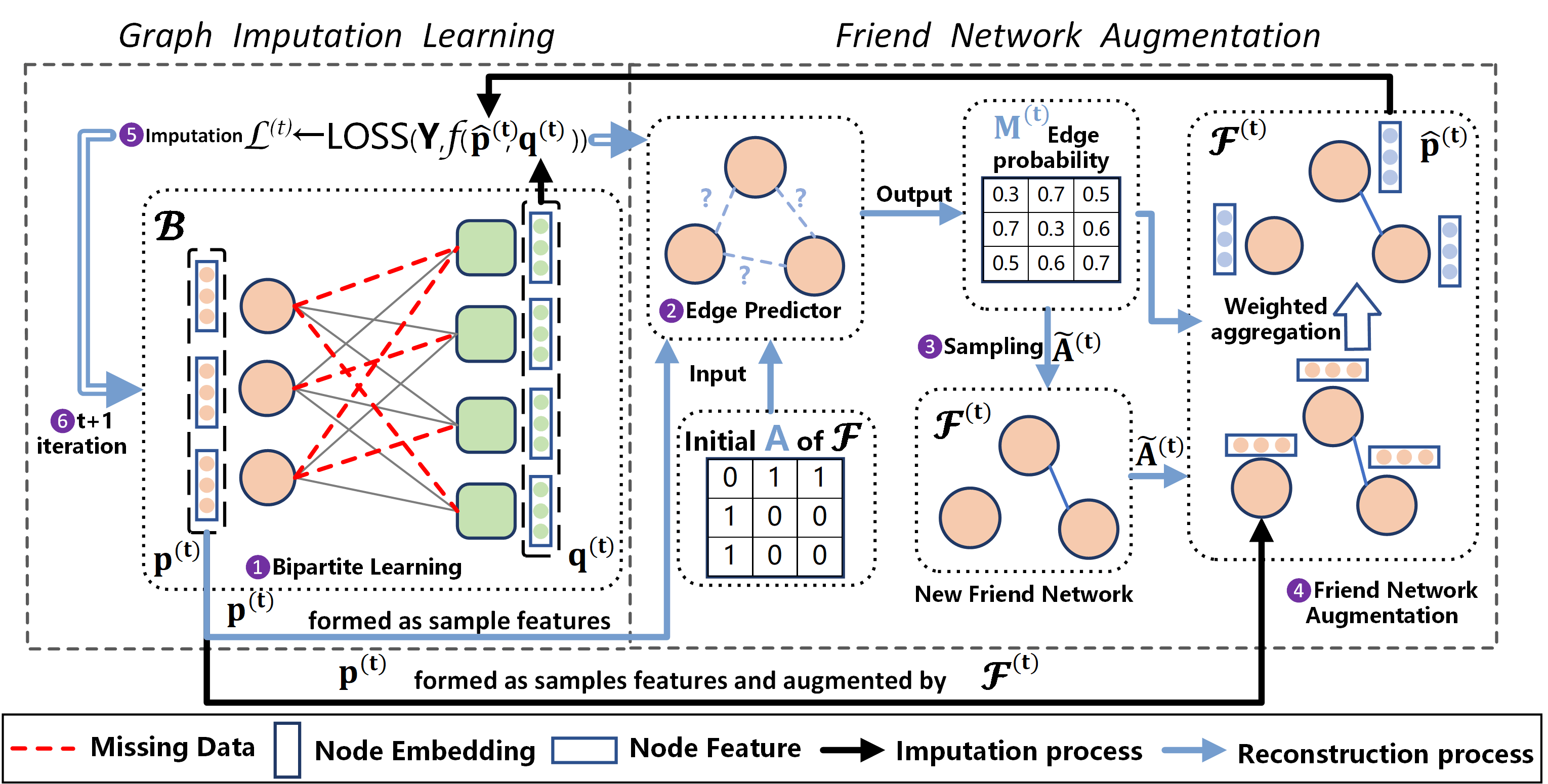
Figure 2: Overall architecture of the proposed IGRM framework in $t$-th iteration.

IGRM

In this section, we propose the basic structure of the IGRM framework and illustrate designs that allow for the end-to-end learning of an accurate friend network under a data matrix with missing.

Network Architecture

Fig.2 shows the overall architecture and training process at $t$-th iteration. IGRM is comprised of two modules: the graph imputation learning module for bipartite graph $\mathcal{B}$ learning (left part of Fig.2) and friend network augmentation module (right part). Existing GNNs solutions only have graph imputation learning module and learn the data imputation model with an edge-level prediction function ${f}$ in the bipartite graph $\mathcal{B}$. The $\hat{D}_{ij}=f_{ij}{(\mathcal{B})}$ by minimizing the difference between $\hat{D}_{ij}$ and ${D}_{ij}$. In comparison, IGRM introduces a novel friend network augmentation module which does not exist in other Graph-based imputation solutions.

In IGRM, the key problem lies in how to generate an accurate friend network under the distribution deviation introduced by the missing data and how can the bipartite graph $\mathcal{B}$ and the friend network $\mathcal{F}$ effectively integrate knowledge from each other. Here, we use the Graph Representation Learning (GRL) (Hamilton, Ying, and Leskovec 2017b) to distill important graph knowledge into dense embeddings from the friend network $\mathcal{F}$. Here, let $\hat{\mathbf{p}}$ represent the sample embeddings distilled from the friend network. Then, the bipartite graph learning can be changed from only the bipartite graph $\mathcal{B}$ to the combination of both $\mathcal{B}$ and $\hat{\mathbf{p}}$.

$$\hat{f}_{ij}(\mathbf{\mathcal{B}},\hat{\mathbf{p}})\rightarrow\hat{\mathbf{D}}_{ij}\ \ \forall N_{ij}=0$$ (3)

On the other hand, $\mathcal{F}$ can be optimized with the support of $\mathcal{B}$. Here, let ${\mathbf{p}}$ represent the sample embeddings distilled from the bipartite graph $\mathcal{B}$. As $\mathbf{p}$ presents the high-level abstraction of samples and can be used as an accurate base for the friend network (re)construction. We can get better ${\mathbf{p}}$ during the GRL training process. We define a function that takes the updated $\mathbf{p}^{(t)}$ to generate an optimized new friend network $\mathbf{\widetilde{A}}^{(t)}$. The friend network augmentation includes network structure augmentation and node feature augmentation. Of course, to avoid possible bias introduced by the missing data, we randomly initialize $\mathcal{F}$ with arbitrary numbers of new edges between samples. The initialization process can generally be replaced with any suitable methods. Here, IGRM can be degraded to an existing solution with no relation discovery, e.g., GRAPE, or with one-round relation discovery, e.g., GINN.

Bipartite Graph Learning

In the bipartite graph, the edges of the bipartite graph carry important non-missing value information. Here, we follow the G2SAT (You et al. 2019) to learn the bipartite graph with a variant of GraphSAGE (Hamilton, Ying, and Leskovec 2017a), which can utilize the edge attributes. The source node embedding $\mathbf{p_{i}}$($\mathbf{q_{j}}$) and edge embedding $\mathbf{e}_{ij}$ are concatenated during message passing:

$$\mathbf{h}^{(l)}_{i}\leftarrow Mean(\sigma(\mathbf{W}^{(l)}\cdot Concat(\mathbf{q}^{(l-1)}_{j},\mathbf{e}^{(l-1)}_{ij})$$ (4)

where $l$ indicates the $l$-th layer, $Mean$ denotes the mean operation with a non-linear transformation $\sigma$, $Concat$ is an operation for concatenation, and $\mathbf{W}$ is the trainable weight. Node embedding is updated by:

$$\mathbf{p}^{(l)}_{i}\leftarrow\sigma(\mathbf{\widehat{W}}^{(l)}\cdot Concat(\mathbf{p}^{(l-1)}_{i},\mathbf{h}^{(l)}_{i}))$$ (5)

where $\mathbf{\widehat{W}}$ is trainable. Edge embedding is updated by:

$$\mathbf{e}^{(l)}_{ij}\leftarrow\sigma(\mathbf{Q}^{(l)}\cdot Concat(\mathbf{e}^{(l-1)}_{ij},\mathbf{p}^{(l)}_{i},\mathbf{q}^{(l)}_{j})$$ (6)

where $\mathbf{Q}$ is the trainable weight. Eq.4, 5 and 6 are shown as step-1 in Fig.2. Let $\mathbf{p}^{(t)}$ and $\mathbf{q}^{(t)}$ be the sample and feature embeddings at the last layer of $t$-th iteration.

Friend Network Augmentation & Learning

During training, the friend network should be continuously optimized from both the structure and the feature perspectives. Then, the optimized friend network should also be encoded to support the bipartite graph learning.

Augmentation.

From the bipartite GRL module, we can obtain the sample embeddings $\mathbf{p}^{(t)}$ for $\mathcal{F}$. These embeddings carry rich information and to some extent, can mitigate the impacts of missing data. Thus, this information is being used to guide the friend network (re)construction process for both feature and structure augmentation.

Feature Augmentation. Instead of using the 1 as features in GRAPE, IGRM uses the vector $\mathbf{p}^{(t)}$ as the feature of friend network $\mathcal{F}$. Let $\hat{\mathbf{X}}^{(t)}$ as the feature matrix of $\mathcal{F}$, we have

$$\hat{\mathbf{X}}^{(t)}=\mathbf{p}^{(t)}$$ (7)

Differentiable Structure Augmentation. Here, we propose a novel structure reconstruction component that can continuously optimize the friend network structure according to $\mathbf{p}^{(t)}$. Here, we use Graph auto-encoder (GAE) (Kipf and Welling 2016) to learn class-homophilic tendencies in edges (Zhao et al. 2021) with an edge prediction pretext task. GAE takes initial $\mathbf{A}$ and $\hat{\mathbf{X}}^{(t)}$ as input and outputs an edge probability matrix $\mathbf{M}^{(t)}$. Of course, GAE can generally be replaced with any suitable models.

$$\mathbf{M}^{(t)}=\sigma(\mathbf{Z}\mathbf{Z}^{T}),\mathbf{Z}=GCN_{1}(\mathbf{A},GCN_{0}(\mathbf{A},\hat{\mathbf{X}}^{(t)}))$$ (8)

where $\mathbf{Z}$ is the hidden embedding learned from the encoder, $\sigma$ is the activation function. Then, $\mathbf{M}^{(t)}$ is the edge probability matrix established by the inner-product decoder. The higher the $M_{ij}$, the higher possibility the sample i and j are similar. Thus, we can use $\mathbf{M}^{(t)}$ to generate the new structure of $\mathcal{F}^{(t)}$. Eq.8 is shown as step-2 in Fig. 2.

However, the sampling process of edges from $\mathbf{M}^{(t)}$, such as $argmax(\mathbf{M}^{(t)})$, would cause interruption of gradient back propagation since samples from a distribution on discrete objects are not differentiable with respect to the distribution parameters(Kusner and Hernández-Lobato 2016). Therefore, for trainable augmentation purpose, we employ Gumbel-softmax reparameterization(Jang, Gu, and Poole 2016; Maddison, Mnih, and Teh 2016) to obtain a differentiable approximation by building continuous relaxations of the discrete parameters involved in the sampling process.

$$\mathbf{\widetilde{A}}^{(t)}=\frac{exp((\log(\mathbf{M}^{(t)}_{ij})+g_{i})/\tau}{\sum^{k}_{j=i}exp((\log(\mathbf{M}^{(t)}_{ij})+g_{j})/\tau)}$$ (9)

where $g_{i}\cdots g_{k}$ are independent and identically distributed samples drawn from Gumbel(0,1) and $\tau$ is the softmax temperature. The friend network is reconstructed as $\mathbf{\mathcal{F}}^{(t)}=(\mathbf{U},\mathbf{\widetilde{A}}^{(t)})$. Eq.9 is shown as step-3.

Representation Learning

In order to let similar samples contribute more useful information, we need to encode the friend network into embeddings so $\mathcal{F}$ can be easily used for the bipartite graph imputation learning. Here, we adopt the well-known GraphSAGE on $\mathbf{\mathcal{F}}^{(t)}$ for representation learning in which nodes use $\mathbf{M}^{(t)}$ to perform weighted aggregation of neighbor information. It takes $\hat{\mathbf{X}}^{(t)}$, $\mathbf{\widetilde{A}}^{(t)}$ and $\mathbf{M}^{(t)}$ as input and outputs the embeddings $\hat{\mathbf{p}}^{(t)}$:

$$\begin{split}&\hat{\mathbf{p}}^{(t)}_{\mathbf{i}}\leftarrow\delta(\mathbf{O}\cdot Concat(\mathbf{p}^{(t)}_{i},\sum_{u_{j}\in\mathcal{N}(i)}\hat{\mathbf{X}}^{(t)}_{j}\mathbf{M}^{(t)}_{ij}))\end{split}$$ (10)

where $\mathbf{O}$ is the trainable weight, $\delta$ is the activation function. Eq.10 is shown as step-4.

Imputation Task

Missing values are imputed with corresponding node embeddings $\hat{\mathbf{p}}^{(t)}$ and $\mathbf{q}^{(t)}$:

$$\mathbf{Y}_{pred}=\sigma(f(Concat(\hat{\mathbf{p}}^{(t)},\mathbf{q}^{(t)})))$$ (11)

We then optimize models with the edge prediction task. The imputation loss $\mathcal{L}$ is:

$$\mathcal{L}=CE(\mathbf{Y}_{pred},\mathbf{Y})+MSE(\mathbf{Y}_{pred},\mathbf{Y})$$ (12)

where $\mathbf{Y}=\{\mathbf{D}_{ij}|\forall\mathbf{N}_{ij}=0\}$, we use cross-entropy (CE) when imputing discrete values and use mean-squared error (MSE) when imputing continuous values. Eq.11 and 12 are shown as step-5. The full process is illustrated in Algorithm 1.

Algorithm 1 General Framework for IGRM

Input: $\mathbf{\mathcal{B}}=(\mathbf{U},\mathbf{V},\mathbf{E})$, $\mathbf{N}$, $\mathbf{A}$, iteration T
Output: $\hat{\mathbf{Y}}$, $\widetilde{\mathbf{A}}$

1:  $\mathbf{X}\leftarrow$ 1 if continuous else ONEHOT

2:  $t\leftarrow 0$

3:  while $t<T$ do

4:     $\mathbf{p}^{(t)},\mathbf{q}^{(t)}\leftarrow GNN_{1}(\mathbf{X},\mathbf{E})$ using Eq.4, 5 and 6

5:     $\hat{\mathbf{X}}^{(t)}=\mathbf{p}^{(t)}$

6:     if reconstruct then

7:        $\mathbf{M}^{(t)}\leftarrow GAE(\mathbf{A},\hat{\mathbf{X}}^{(t)})$ using Eq.8

8:        $\widetilde{\mathbf{A}}^{(t)}\leftarrow Sampling(\mathbf{M}^{(t)})$ using Eq.9

9:     end if

10:     $\hat{\mathbf{p}}^{(t)}\leftarrow GNN_{2}(\hat{\mathbf{X}}^{(t)},\widetilde{\mathbf{A}}^{(t)},\mathbf{M}^{(t)})$ using Eq.10

11:     $\mathbf{Y}_{pred}=\sigma(f(CONCAT(\hat{\mathbf{p}}^{(t)},\mathbf{q}^{(t)})))$

12:     $\mathcal{L}=CE(\mathbf{Y}_{pred},\mathbf{Y})+MSE(\mathbf{Y}_{pred},\mathbf{Y})$

13:     $t\leftarrow t+1$

14:  end while

Experiments

Experimental Setup

Dataset

We evaluate IGRM on eight real-world datasets from the UCI Machine Learning repository (Asuncion and Newman 2007) and Kaggle. The first four datasets come from UCI and others come from Kaggle. These datasets consist of mixed data types with both continuous and discrete variables and cover different domains: biomedical(Heart, Diabetes), E-commerce, finance(DOW30), etc. The summary statistics of these datasets are shown in Table 1.

Table 1: Properties of eight datasets, Disc. short for discrete, Cont. short for continuous, and F. short for features.

Dataset	Samples #	Disc. F. #	Cont. F. #
Concrete	1030	0	8
Housing	506	1	12
Wine	1599	0	11
Yacht	308	0	6
Heart	1025	9	4
DOW30	2448	0	12
E-commerce	10999	7	3
Diabetes	520	15	1

Baseline models

We compare IGRM against nine commonly used imputation methods, including statistical methods and machine learning models. The implementations used are mainly from respective papers. Mean: a feature-wise mean imputation. KNN (Hastie et al. 2015): the mean of the K-nearest observed neighbors as imputation. MICE (Buuren and Groothuis-Oudshoorn 2010): provides multiple imputation values for each missing value with different missing assumptions. SVD (Troyanskaya et al. 2001): imputes data by performing single value decomposition on the dataset. Spectral (Mazumder, Hastie, and Tibshirani 2010): imputes data with a soft-thresholded SVD. GAIN (Yoon, Jordon, and Schaar 2018): imputes data using Generative Adversarial Nets. OT (Muzellec et al. 2020): a deep neural distribution matching method based on optimal transport (OT). Here, the Sinkhorn variant is chosen. Miracle (Kyono et al. 2021): a causally-aware imputation framework. GINN (Spinelli, Scardapane, and Uncini 2020): an imputation framework based on the graph denoising autoencoder. GRAPE (You et al. 2020):a pure bipartite graph-based framework for feature imputation.

Table 2: Comparisons of averaged(*10) MAE values for missing data imputation on eight datasets with 30% and 70% MCAR. Results are enlarged by 10 times. Results for MAR and MNAR hold similar trends and can be found in Appendix

Dataset	Concrete		Housing		Wine		Yacht		Heart		DOW30		E-commerce		Diabetes
Ratio	30%	70%	30%	70%	30%	70%	30%	70%	30%	70%	30%	70%	30%	70%	30%	70%
Mean	1.83	1.81	1.82	1.82	0.98	0.98	2.14	2.18	2.33	2.33	1.53	1.53	2.51	2.51	4.37	4.35
KNN	1.25	1.74	0.96	1.52	0.80	1.11	2.18	2.72	1.11	2.35	0.40	1.11	2.76	2.83	2.57	4.09
MICE	1.36	1.73	1.16	1.61	0.76	0.93	2.09	2.25	2.04	2.27	0.59	1.22	2.43	2.57	3.32	4.00
SVD	2.15	2.26	1.44	2.11	1.08	1.27	2.80	3.26	2.43	3.03	0.94	1.55	2.75	3.06	3.64	4.36
Spectral	2.01	2.56	1.44	2.21	0.92	1.45	2.94	3.58	2.34	3.04	0.78	2.01	3.10	3.64	3.97	4.71
GAIN	1.52	1.87	1.35	1.74	0.92	1.06	13.28	13.31	2.20	2.31	1.23	1.48	2.61	2.59	3.40	3.85
OT	1.18	1.76	0.91	1.29	0.78	1.02	1.75	2.57	1.82	2.15	0.44	0.85	2.57	2.58	2.50	3.60
Miracle	1.30	1.90	1.11	2.50	0.73	1.66	1.88	4.89	2.03	4.23	0.62	2.86	2.43	3.31	3.62	7.50
GINN	1.68	1.56	1.63	1.69	1.17	0.96	1.80	2.10	1.95	1.81	1.50	1.37	2.67	2.93	4.28	4.10
GRAPE	0.86	1.67	0.76	1.21	0.63	0.93	1.61	2.35	1.55	2.23	0.20	0.50	2.35	2.51	2.49	3.91
IGRM	0.74	1.42	0.69	1.02	0.62	0.92	1.11	2.05	1.51	2.24	0.18	0.27	2.27	2.41	2.41	3.69

Table 3: Ablation study. The time reported here is the initialization time(seconds) of friend network in Concrete.

Dataset	Concrete	Housing	Wine	Yacht	Heart	DOW30	E-commerce	Diabetes	Time
IGRM	0.74$\pm 0.01$	0.69$\pm 0.01$	0.62$\pm 0.00$	1.11$\pm 0.07$	1.51$\pm 0.01$	0.18$\pm 0.01$	2.27$\pm 0.01$	2.41$\pm 0.02$	0.01
w/o GAE	0.86$\pm 0.01$	0.80$\pm 0.02$	0.64$\pm 0.00$	1.63$\pm 0.06$	1.62$\pm 0.01$	0.20$\pm 0.00$	2.35$\pm 0.01$	2.68$\pm 0.04$	0.01
once GAE	0.80$\pm 0.01$	0.73$\pm 0.02$	0.63$\pm 0.01$	1.33$\pm 0.04$	1.57$\pm 0.07$	0.20$\pm 0.00$	2.31$\pm 0.02$	2.56$\pm 0.08$	0.01
IGRM-cos	0.76$\pm 0.01$	0.70$\pm 0.01$	0.63$\pm 0.01$	1.29$\pm 0.04$	1.50$\pm 0.01$	0.19$\pm 0.01$	2.27$\pm 0.01$	2.38$\pm 0.03$	86.50
IGRM-rule	0.76$\pm 0.00$	0.69$\pm 0.01$	0.62$\pm 0.01$	1.09$\pm 0.01$	1.55$\pm 0.03$	0.19$\pm 0.01$	2.27$\pm 0.00$	2.40$\pm 0.04$	12.99

Parameter settings

For all baselines, we follow their default settings from their papers. IGRM employs three variant GraphSAGE layers with 64 hidden units for bipartite GRL and one GraphSAGE layer for friend network GRL. The Adam optimizer with a learning rate of 0.001 and the ReLU activation function is used. In the process of initializing $\mathcal{F}$, we randomly connect samples with sample size $|\mathbf{U}|$ edges to build the initial friend network. This structure of the friend network is reconstructed per 100 epochs during the bipartite graph training. As the datasets are completely observed, we introduce certain percentages of missing data with missing with complete random mask(MCAR), missing at random (MAR), and missing not at random (MNAR) with different missing ratios. We treat the observed values as train set and missing values as the test set. Values are scaled into $[0,1]$ with the MinMax scaler (Leskovec, Rajaraman, and Ullman 2020). For all experiments, we train IGRM for 20,000 epochs, run five trials with different seeds and report the mean of the mean absolute error(MAE). Due to page limits, results for MAR and MNAR with settings (Muzellec et al. 2020) are shown in Appendix.

Experimental Results

Table 2 shows the mean of MAE compared with various methods with 30% and 70% missing ratios, the best result is marked in bold, and the second is underlined. For 30% missing, IGRM outperforms all baselines in 7 out of 8 datasets and reaches the second best performance in Heart, and its MAE is 2%~31% lower compared with the best baseline GRAPE. Mean imputation only uses a single dimension of features for imputation and reaches almost the worst results. SVD and Spectral highly depend on certain hyper-parameters, which results in erratic performance across different datasets, even worse results in 5 datasets than Mean. GAIN is also not stable. It has the most significant variance and gets the worst result in Yacht. GRAPE explicitly models the pure bipartite graph and learns highly expressed representations of observed data. Its performance is comparably stable and usually ranks second. However, it fails to get weights from similar samples. IGRM introduces a friend network based on the pure bipartite graph, encouraging information propagation between similar samples, which is beneficial for imputation. Furthermore, the performances of most baselines are worse than Mean under the 70% missing ratio, while IGRM still maintains good performance.

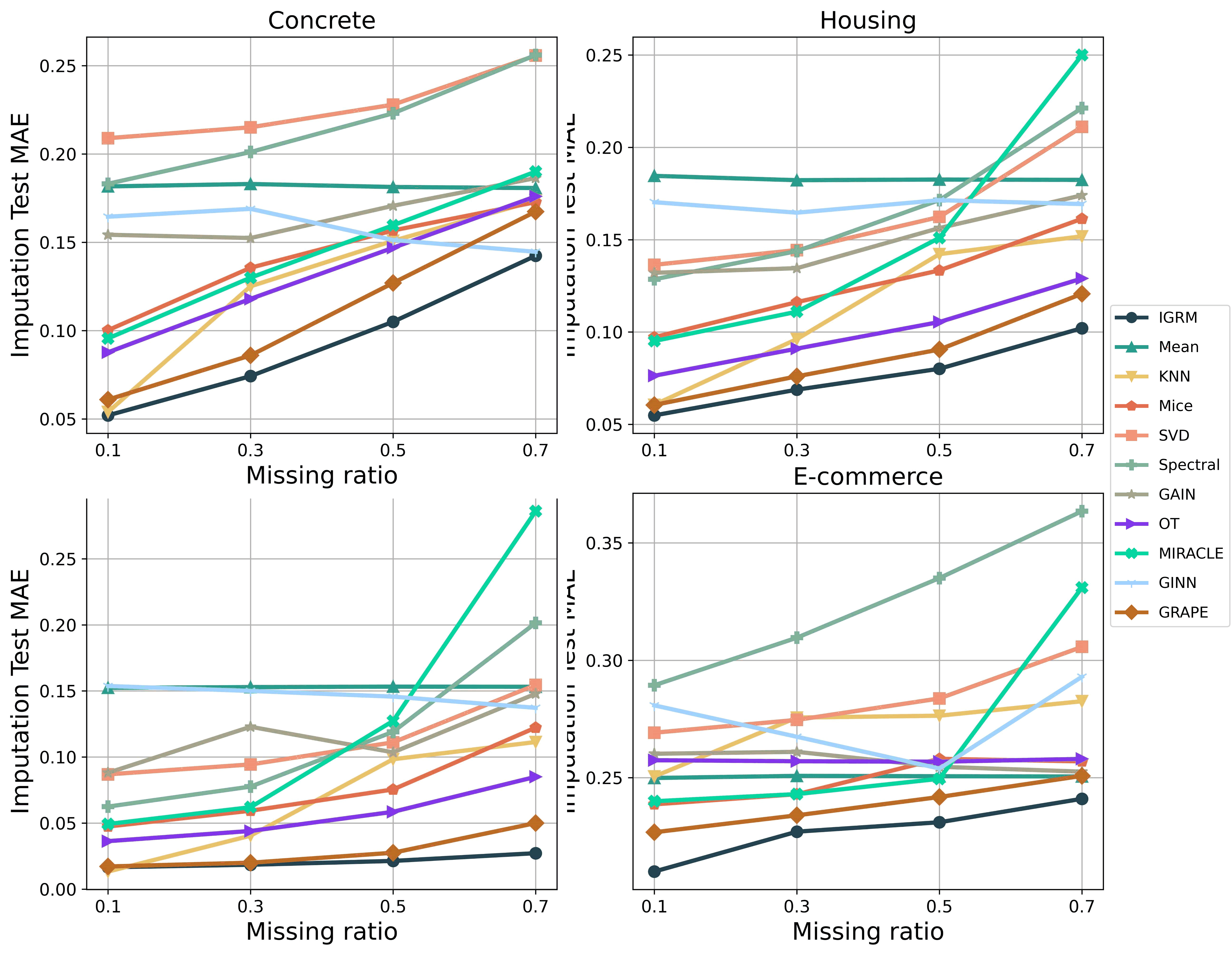
Figure 3: Averaged MAE of feature imputation with different missing ratios over five trials.

Different missing ratio

To examine the robustness of IGRM with respect to the missing ratios of the data matrix: 0.1,0.3,0.5,0.7. The curves in Fig.3 demonstrate the trends of all methods. With the increase of the missing ratio, the performance of almost all algorithms except for Mean, generally decreases. In comparisons, IGRM consistently outperforms other baselines across almost the entire range of missing ratios. In the missing ratio of 0.1, KNN also performs well. A possible explanation for these results is that low missing ratios do not significantly distort the clustering results. However, KNN suffers significant performance deterioration with a high missing ratio due to the large similarity deviation from missing data. While IGRM relieves the problem of data sparse by constructing the friend network.

Embedding Evaluation

In this section, we evaluate the qualities of generated sample embeddings from IGRM.

Quality of embeddings

We visualize sample embeddings of IGRM and GRAPE with t-SNE (Laurens and Hinton 2008) and calculate the average silhouette score (Rousseeuw 1987) for all sample embeddings. We compare them with the clusters generated with the ground-truth complete tabular data. The higher value of the silhouette score means embeddings are better separated. Fig.4 shows the embeddings distribution in Yacht. We can observe that IGRM tends to be better clustered and have clearer boundaries between classes than GRAPE. IGRM has a silhouette score of 0.17, about 35.7% higher than 0.14 in GRAPE. As a result, IGRM achieves a MAE 31% lower than GRAPE.

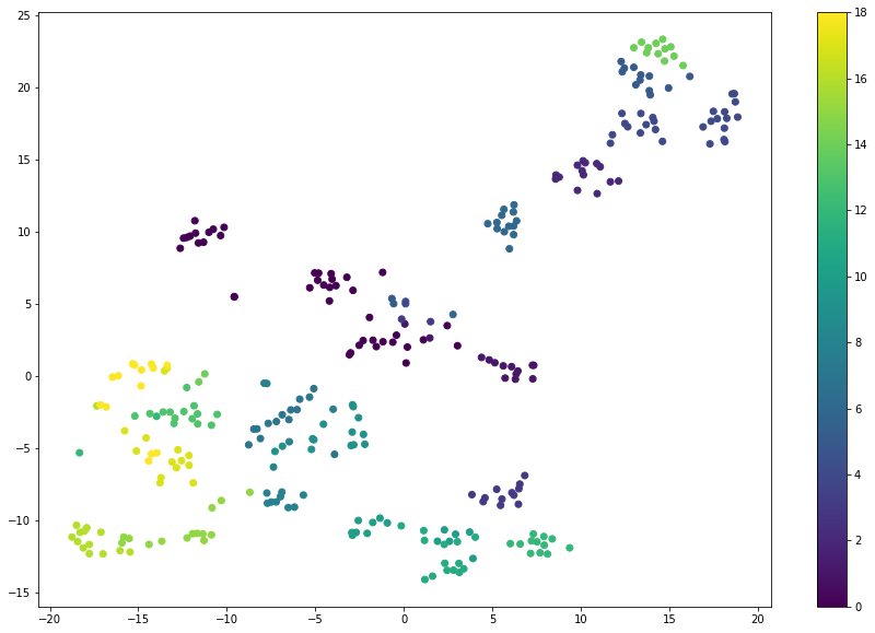
(a) IGRM-Yacht(0.17)

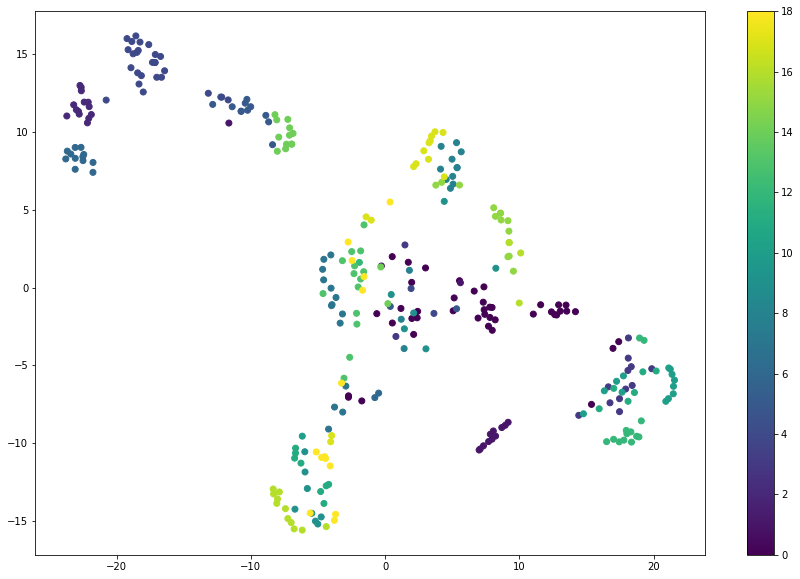
(b) GRAPE-Yacht(0.14)

Figure 4: The t-SNE embeddings of nodes from IGRM and GRAPE. The value in () indicates the silhouette coefficient.

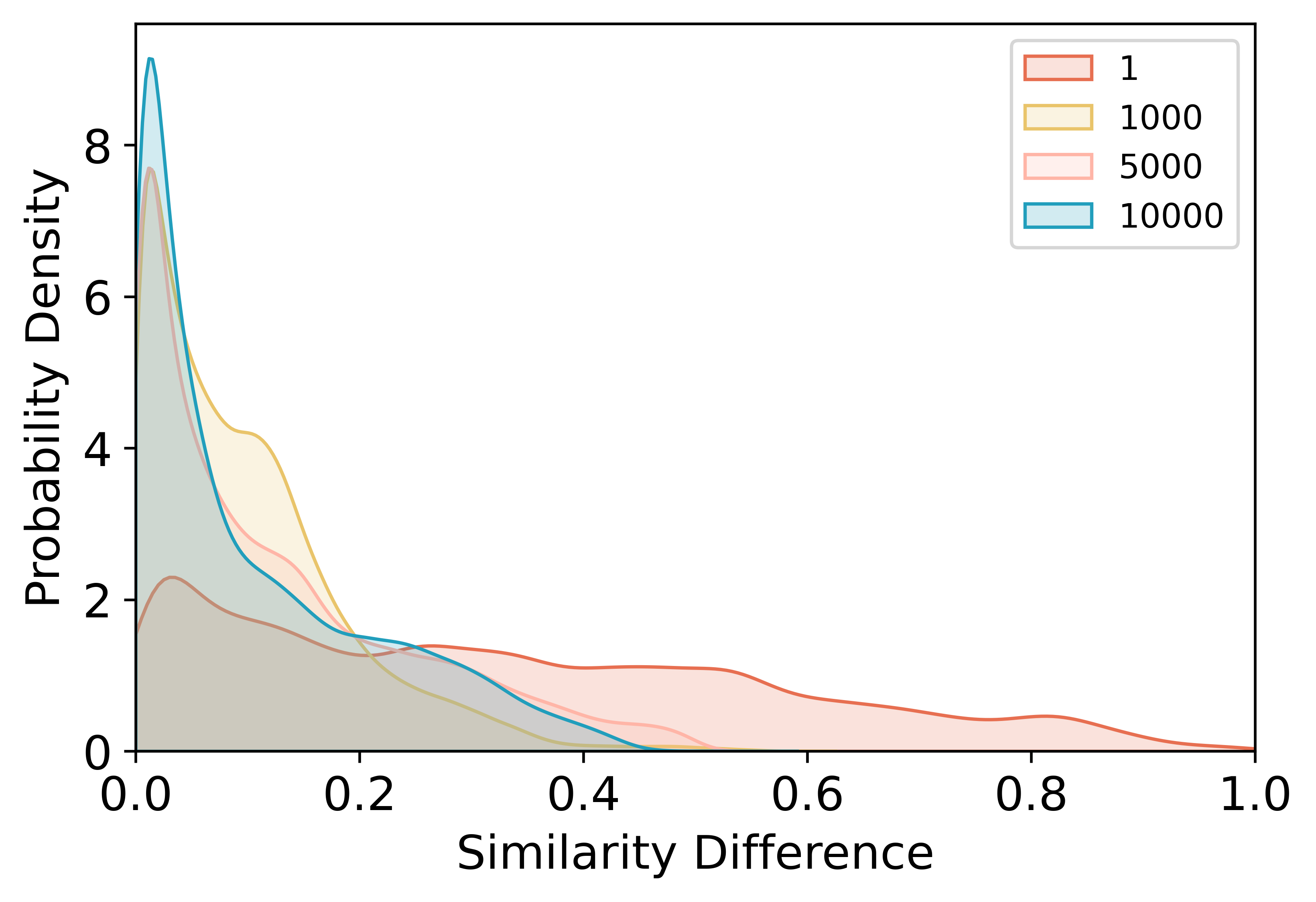
(a) DOW30

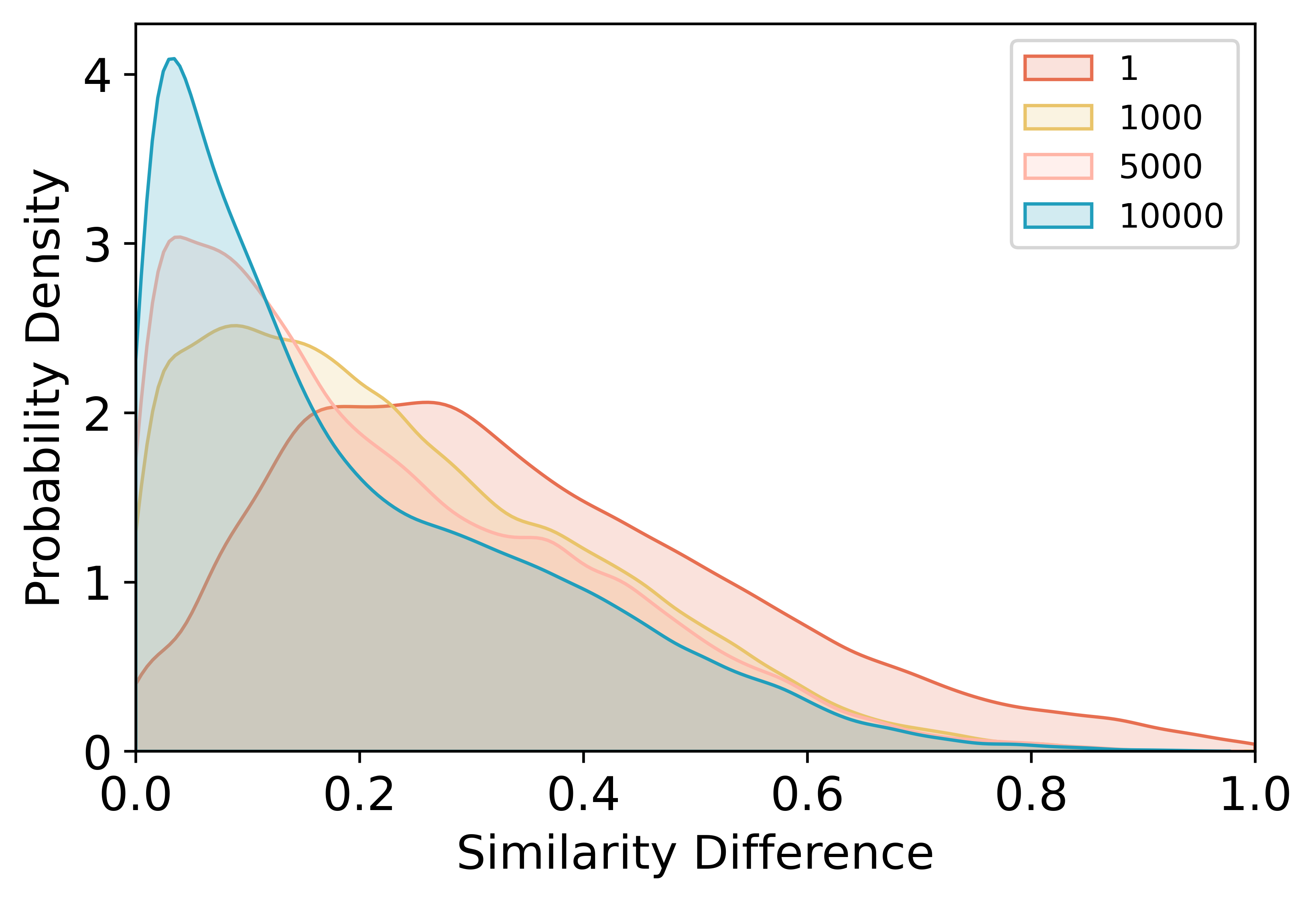
(b) Yacht

Figure 5: Trends of similarity deviation distribution during training with missing ratio 0.3. The deviation is the absolute value of the difference between the generated embeddings similarity and the ground-truth similarity.

Evolution of embeddings

To prove the effectiveness of iterative friend network reconstruction, we show the cosine similarity deviation distribution at 1st, 1,000th, 5,000th, and 10,000th epoch in DOW30 and Yacht with missing ratio 0.3. Fig.5 shows that the quality of generated embeddings gradually improves during the training process. The similarity deviation in the 1st epoch is relatively high with most distributed around 0.3$\sim$0.6 and a few less than 0.2. During training, the quality of the embeddings is much improved. The similarity of node embeddings at the 5,000th epoch is already highly close to the ground truth. It verifies the effectiveness of the iterative friend network reconstruction.

Ablation Study

In this subsection, we study the impact of different designs and show their impacts on the data imputation.

Impacts from friend network reconstruction.

We test the performance with the friend network reconstruction component turned off(w/o GAE) or only reconstructing the friend network once at the first epoch(once GAE). The results are shown in Table. 3. IGRM(w/o GAE) suffers significant performance deterioration consistently on all datasets, sometimes even worse than GRAPE. We conjecture this is because the initial random-generated friend network is very noisy. Training on a random friend network without reconstruction can hardly helpful. With even one reconstruction, IGRM(once GAE) achieves significant performance improvements over IGRM(w/o GAE) across almost all tested datasets. This result clearly shows the effectiveness of friend network reconstruction. For the iterative reconstruction, almost all compared datasets show further improvements when the friend network is optimized iteratively, compared to IGRM(once GAE). Results demonstrate that the friend network at the early stage is inaccurate, and the iterative reconstruction is essential for IGRM,

Impacts of friend network initialization.

We further investigate how the friend network’s initialization method(random, rule, cos) affects IGRM’s performance. IGRM-cos calculates the exploits cosine similarity among samples and connects the most similar sample pairs with the same number of IGRM-random. IGRM-rule uses FP-growth (Han, Pei, and Yin 2000) to mind frequent data patterns in samples and connects samples failing in the same rule. In IGRM-rule, we discrete the continuous data with Davies-Bouldin index (Davies and Bouldin 1979) to handle continuous features. Detailed descriptions of the IGRM-rule can be found in Appendix. The lower part of Table. 3 shows three methods have no significant performance differences while the random initialization is about four orders faster. The complexity of IGRM-rule is $\mathcal{O}(nlogn)$ and even higher $\mathcal{O}(n^{2})$ for IGRM-cos. As the iterative reconstruction process can largely mitigate the importance of friend network initialization, IGRM uses random initialization as default.

Network reconstruction frequency

One of the major overheads introduced by IGRM is the friend network reconstruction. Table. 4 shows the effect of friend network reconstruction with different update frequencies(per 1/10/100 epochs). The speedup ratio is the time spent with reconstruction per 1 epoch divided by reconstruction with other frequencies. Results before / are time ratio between per 1 and 10 epochs and after are time ratio between per 1 and 100 epochs. With different update frequency, the imputation results largely unchanged. However, a large speed up is observed when per 100 epochs is used, especially for big datasets, e.g. E-commerce. Therefore, IGRM reconstructs the friend network per 100 epochs.

Table 4: Results and speedup v.s network update frequency.

Per # Epoch	1	10	100	Speedup
Concrete	0.76$\pm 0.01$	0.74$\pm 0.01$	0.74$\pm 0.02$	4.36/6.53
Housing	0.69$\pm 0.01$	0.68$\pm 0.01$	0.69$\pm 0.01$	1.51/2.03
Wine	0.62$\pm 0.01$	0.61$\pm 0.00$	0.62$\pm 0.01$	4.16/6.24
Yacht	1.12$\pm 0.09$	1.06$\pm 0.07$	1.11$\pm 0.08$	1.71/1.92
Heart	1.60$\pm 0.03$	1.52$\pm 0.03$	1.51$\pm 0.03$	3.18/4.37
DOW30	0.19$\pm 0.00$	0.19$\pm 0.00$	0.18$\pm 0.01$	5.37/9.40
E-commerce	2.28$\pm 0.01$	2.27$\pm 0.01$	2.27$\pm 0.00$	8.22/27.48
Diabetes	2.42$\pm 0.03$	2.45$\pm 0.03$	2.41$\pm 0.04$	1.93/2.14

Conclusion

In this paper, we propose IGRM, an iterative graph generation and reconstruction based missing data imputation framework. First, we transform the missing data imputation problem into an edge-level prediction problem. And under the assumption that similar nodes would have similar embeddings, we cast the similarity relations modeling problem in sample nodes as node embeddings similarity problem. IGRM jointly and iteratively learning both friend network structure and node embeddings optimized by and for the imputation task. Experimental results demonstrate the effectiveness and efficiency of the proposed model. In the future, we plan to explore effective techniques for handling the missing data problem in large datasets.

APPENDIX

MAR and MNAR

The missing mechanisms are traditionally divided into three categories according to the data distribution: missing completely at random (MCAR), missing at random (MAR), and missing not at random (MNAR) (Little and Rubin 1987). In MCAR, the missing of a value is completely random and does not depend on any other values. In MAR, the missing of a value is only correlated with other observed values while in MNAR, the missing is related to both missing values and observed values.

In this section, we introduce the implementation of MAR and MNAR mechanisms and provide additional experiments based on MAR and MNAR mechanisms.

Experiments Settings.

In MAR setting, for each dataset, we sample a fixed subset of features which would be introduced missing values and the remaining of the features would have no missing value. Then the missingness would be masked in the fixed subset of features according to the logistic masking model with random weights which takes the features have no missing values as input and outputs a binary mask matrix.

In MNAR setting, for each dataset, we also sample a fixed subset of features which would have missing values according to the logistic masking model with random weights. While this logistic masking model takes the remaining features as input and outputs the binary mask matrix. Finally, the remaining features would be masked by MCAR mechanism.

Table 1: Comparisons of average(*10) and variance of MAE values for missing data imputation on eight datasets with 30% and 70% missing ratio of 50% features with MAR. Results have been enlarged by 10 times for better display effects

Models	Concrete		Housing		Wine		Heart		DOW30		E-commerce		Diabetes		Yacht
Ratio	30%	70%	30%	70%	30%	70%	30%	70%	30%	70%	30%	70%	30%	70%	30%	70%
Mean	1.72	1.73	1.98	1.85	1.04	1.00	2.37	2.36	1.49	1.49	2.68	2.69	4.30	4.41	2.00	2.13
KNN	0.61	0.98	0.71	0.82	0.60	0.76	0.40	1.23	0.16	0.21	2.79	2.84	1.29	2.11	1.67	1.86
MICE	1.08	1.38	1.07	1.19	0.73	0.80	2.01	2.18	0.60	0.69	2.58	2.69	3.00	3.50	1.44	1.77
SVD	2.21	2.51	1.49	1.84	1.30	1.37	2.51	2.95	1.03	1.19	2.85	2.92	3.44	3.79	2.54	2.74
Spectral	1.80	2.36	1.37	1.84	0.91	1.37	2.31	2.93	0.74	1.36	2.97	3.28	4.00	4.94	2.09	2.82
GAIN	1.39	1.81	1.27	1.44	0.89	0.88	2.16	2.31	0.81	0.92	2.62	2.38	3.36	3.65	12.17	7.41
OT	1.09	1.54	0.86	1.15	0.77	0.86	1.84	2.09	0.43	0.68	2.56	2.51	2.51	3.29	1.68	2.53
Miracle	0.97	1.46	1.29	1.71	0.78	0.85	1.98	2.53	1.70	3.86	2.40	2.75	3.13	3.29	1.90	2.53
GRAPE	0.65	0.98	0.71	0.84	0.64	0.71	1.35	1.81	0.19	2.26	2.56	2.82	1.98	2.75	1.41	1.84
IGRM	0.60	0.81	0.59	0.75	0.61	0.68	1.28	1.72	0.18	0.21	2.31	2.34	1.89	2.55	0.66	1.17

Table 2: Comparisons of average(*10) and variance of MAE values for missing data imputation on eight datasets with 30% and 70% missing ratio of 50% features with MNAR. Results have been enlarged by 10 times for better display effects

Models	Concrete		Housing		Wine		Heart		DOW30		E-commerce		Diabetes		Yacht
Ratio	30%	70%	30%	70%	30%	70%	30%	70%	30%	70%	30%	70%	30%	70%	30%	70%
Mean	1.84	1.84	1.94	1.87	1.02	1.00	2.34	2.34	1.57	1.58	2.51	2.51	4.38	4.44	2.11	2.20
KNN	1.40	1.81	1.21	1.68	1.03	1.17	1.39	2.41	0.50	1.20	2.88	2.88	2.61	4.27	1.99	2.87
MICE	1.37	1.78	1.23	1.66	0.80	0.94	2.08	2.27	0.61	1.26	2.43	2.58	3.21	4.09	1.64	2.21
SVD	2.21	2.69	1.51	2.39	1.17	1.39	2.52	3.23	1.00	1.67	2.76	3.15	3.57	4.53	2.68	3.47
Spectral	1.96	2.52	1.46	2.35	0.92	1.48	2.37	3.11	0.76	1.98	3.09	3.66	4.08	5.10	2.57	3.74
GAIN	1.68	1.86	1.62	1.80	0.93	1.48	2.37	3.11	0.76	1.98	3.09	3.66	4.08	5.10	2.57	3.74
OT	1.16	1.76	0.90	1.34	0.77	1.01	1.81	2.11	0.47	0.89	2.54	2.53	2.55	3.65	1.77	2.48
Miracle	1.30	2.07	1.38	3.01	0.74	1.71	2.05	4.32	1.11	3.35	2.44	3.47	3.37	7.73	1.95	5.66
GRAPE	0.92	1.64	0.77	1.25	0.67	0.90	1.58	2.13	0.20	0.48	2.30	2.47	2.41	3.63	1.49	2.33
IGRM	0.82	1.38	0.67	1.08	0.66	0.87	1.54	2.11	0.20	0.29	2.27	2.35	2.25	3.36	1.06	2.00

Experimental Results.

Table 1 and 2 show the mean of MAE compared with various methods with 30% and 70% missing ratios in MAR and MNAR mechanisms, the best result is marked in bold and the results have been enlarged by 10 times. In MNAR mechanism, IGRM outperforms all baselines in 6 out of 8 datasets and reaches the second best performance in Heart dataset and comparable result in DOW30 dataset. IGRM yields 7.77% and 12.46% lower mean MAE than the second-best baseline(GRAPE) in 30% and 70% missing respectively. While in MAR mechanism, IGRM outperforms baselines except KNN in 4 datasets and reaches the best performance in the remaining datasets. We conjecture this is because, in MAR setting, a subset of features have no missing values, through which KNN can capture similar neighbors accurately. Results show that IGRM performs well and is robust to difficult missing mechanisms, this is remarkable as IGRM do not attempt to be designed for these missing mechanisms. In addition, IGRM can also perform well in 70% missing ratios in both MAR and MNAR mechanisms while the performances of other baselines are usually worse than Mean imputation. This further confirms that the introduction of friend network can effectively alleviate the problem of data sparsity.

Additional Evolution of Embeddings

In this section, to further prove the effectiveness of iterative friend network reconstruction, we show additional cosine similarity deviation evolution during iterative learning at 1st, 1000th, 5000th, 10000th epoch in several datasets. Results illustrated in Fig. 1 further prove that embeddings can gradually mitigate the effect of missing data during the model training.

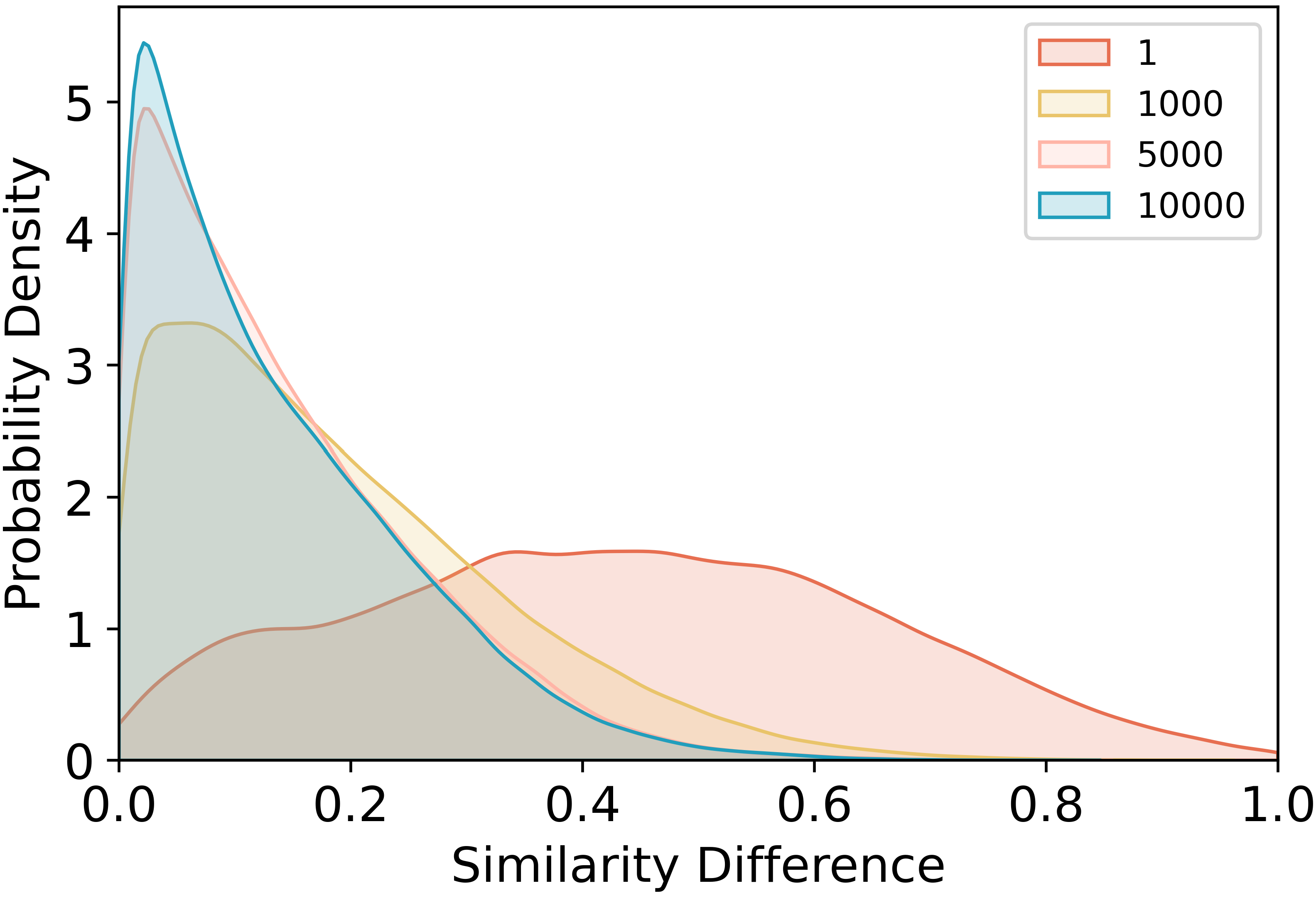
(a) Concrete

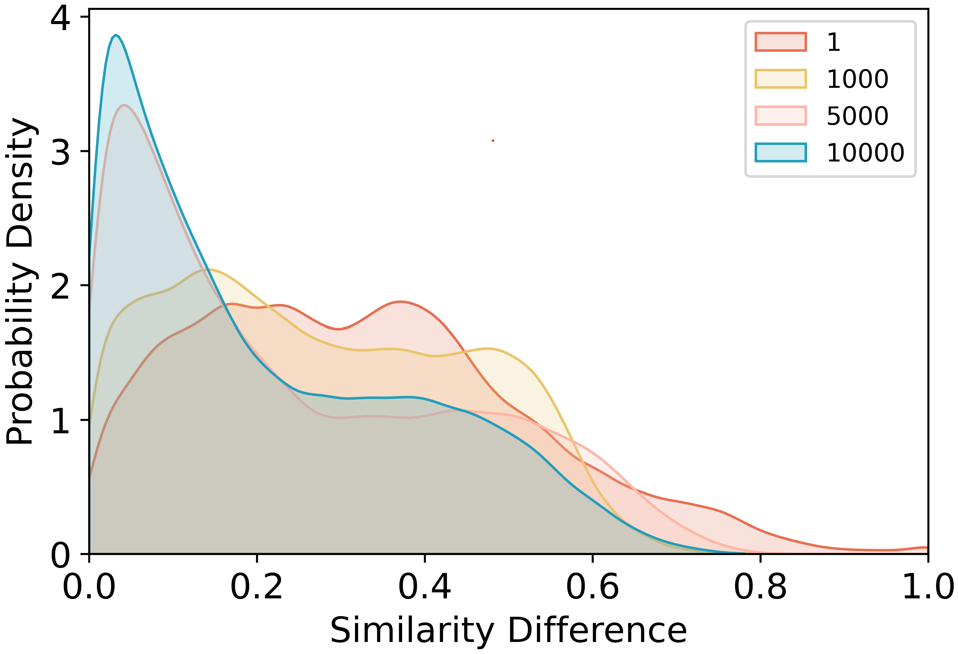
(b) Housing

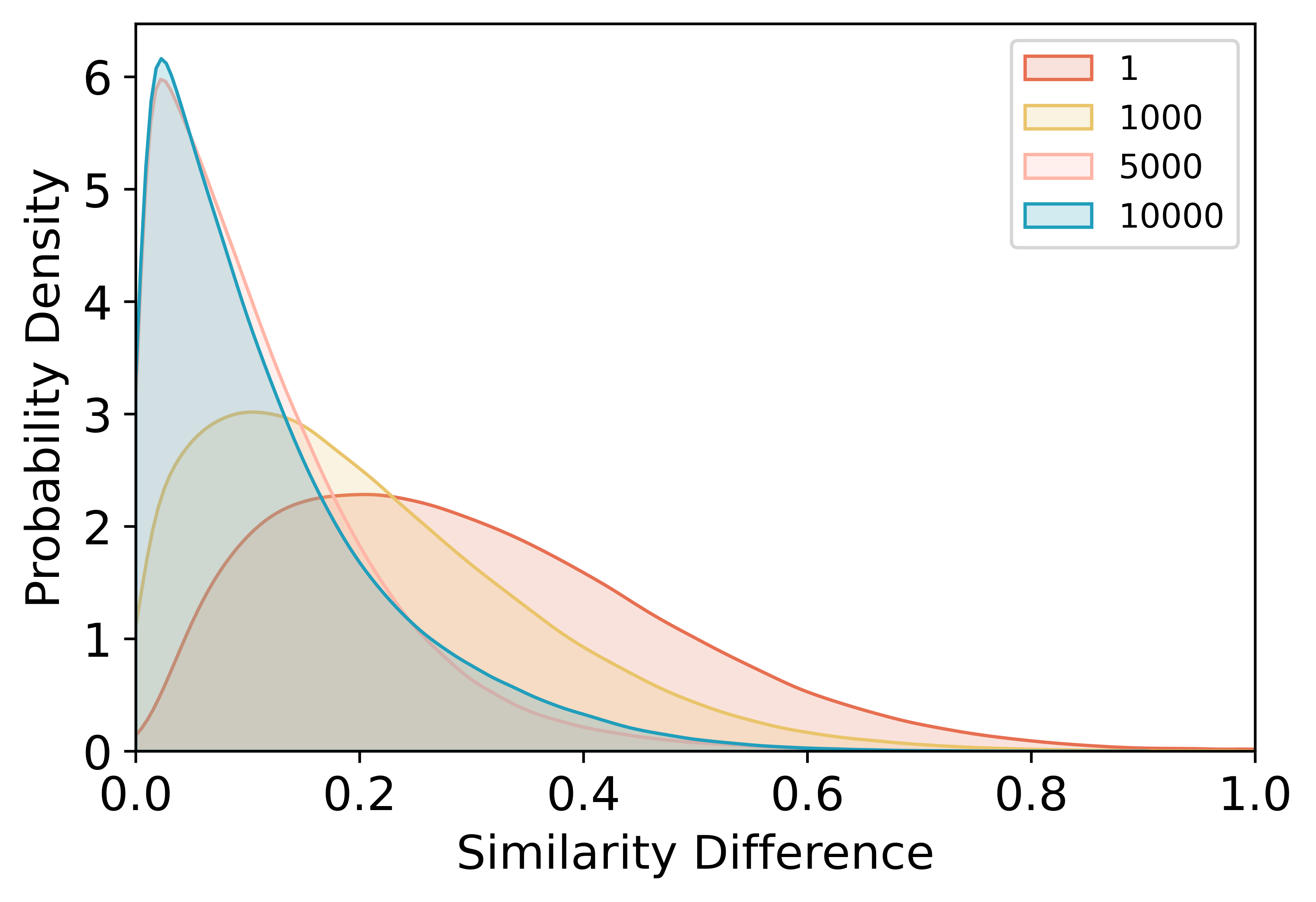
(c) Wine

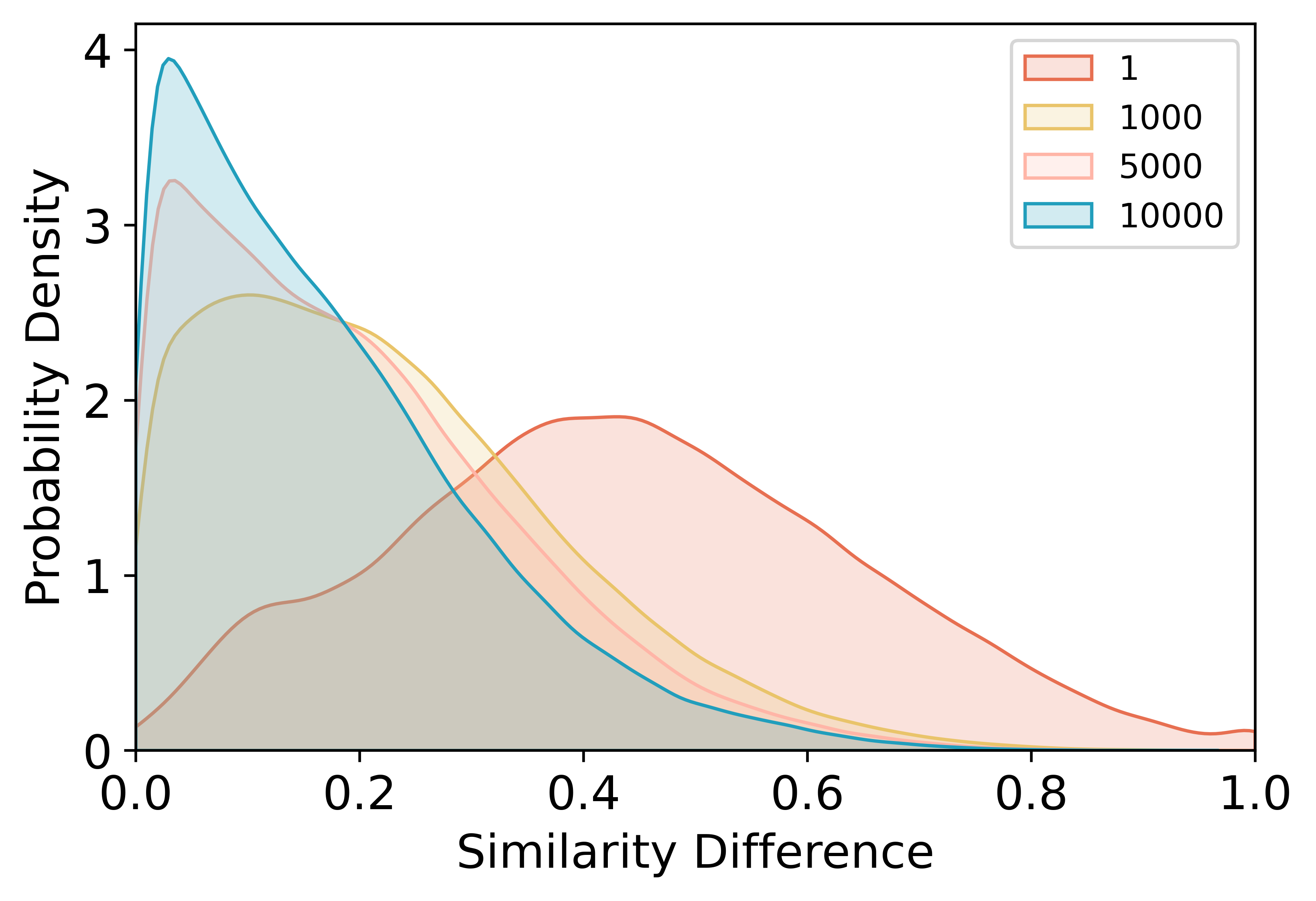
(d) Heart

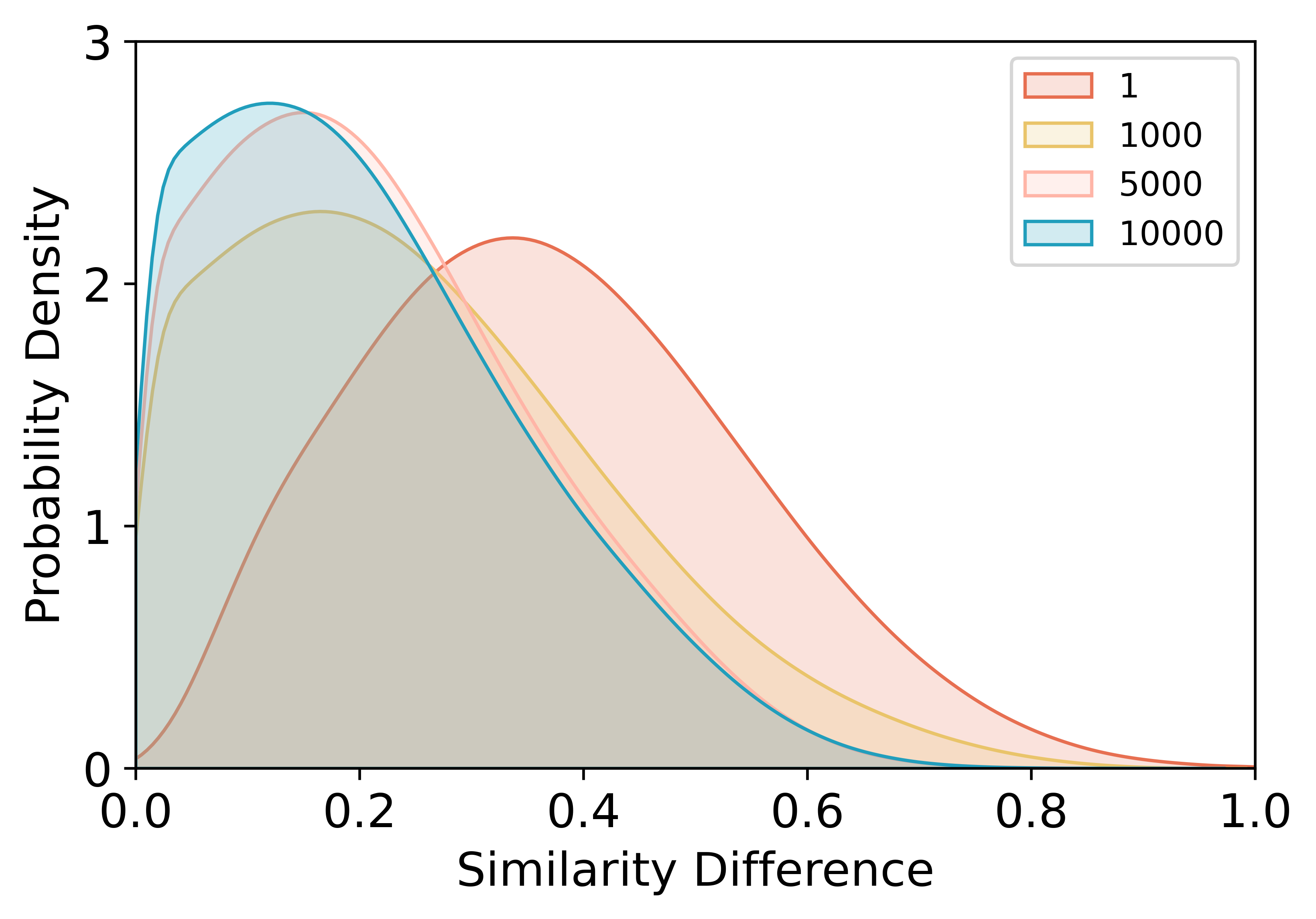
(e) E-commerce

(f) Diabetes

Figure 1: Similarity deviation distribution. The deviation is the absolute value of the difference between the generated embeddings similarity and the ground-truth similarity.

Additional Experiments

In this section, we provide some additional experiments on more datasets come from UCI (Asuncion and Newman 2007). The summary statistics of datasets are shown in Table 3. The results are shown in Fig. 2. Results have been normalized by the average performance of Mean imputation for better display effects.

Results show that IGRM yields 12.93%, 16.93% and 23.67% lower mean of MAE than the second-best baselines in MCAR, MAR and MNAR mechanisms respectively. In addition, IGRM outperforms all baselines in all datasets in MCAR mechanisms and it outperforms baselines except KNN and MICE in Ai4i dataset in MAR mechanism.

Dataset	Blood	Steel	Phoneme	Abalone	Energy	Cmc	German	Ai4i
Samples #	748	1941	5404	4177	768	1473	1000	10000
Disc. F. #	0	0	0	1	0	8	13	7
Cont. F. #	4	33	5	7	8	1	7	5

Table 3: Properties of additional datasets used in experiments, Disc. short for Discrete and Cont. short for continuous.

Figure 2: Imputation methods on 8 datasets from the UCI repository in 30% missing in MCAR(top), MAR(middle), MNAR(bottom) mechanisms. The result is normalized by the average performance of Mean imputation.

Initialization Method Details

In this section, we provide details about the initialization of IGRM-rule.

IGRM-rule

is initialized by association rules, since we consider that two samples with the same rules are similar in feature sub-spaces. Since majority of our datasets have mixed data types, before mining rules, the continuous features of $\mathbf{D}$ is discretized by the cluster binning technique which is determined by Davies-Bouldin index(Davies and Bouldin 1979), resulted in $\hat{\mathbf{D}}$. In this work, we adopt FP-growth(Han, Pei, and Yin 2000) to mine the frequent itemsets in observed values, and set the default minimum support and confidence as 0.1 and 0.6 respectively while in Housing dataset the minimum confidence is 0.7 and in E-commerce dataset the minimum confidence is 0.5 to obtain association rules. An association rule can be formed as $\mathcal{R}:\mathbf{A}\Rightarrow\mathbf{B}$, where $\mathbf{A}$ is antecedent and $\mathbf{B}$ is consequent, $\mathbf{A}\cap\mathbf{B}=\varnothing$. The items in $\mathbf{A}$ and $\mathbf{B}$ are denoted as $a_{1},a_{2},...,a_{n}$ and $b$.

Candidate node set $\mathbf{C}$ contains sample nodes whom both $\mathbf{A}$ and $\mathbf{B}$ exist in, $\mathbf{C}=\{u_{i}|(\mathbf{A}\cup\mathbf{B})\subseteq\{\mathbf{D}_{ij}|\mathbf{N}_{ij}=1,j=1,...,m\}\}$. For each time, we sample and connect a pair of nodes without replacement from $\mathbf{C}$, repeats this work until $\mathbf{C}$ is empty.

References

- Acuna and Rodriguez (2004) Acuna, E.; and Rodriguez, C. 2004. The treatment of missing values and its effect on classifier accuracy. In Classification, clustering, and data mining applications, 639–647. Springer.
- Allen and Li (2016) Allen, A.; and Li, W. 2016. Generative adversarial denoising autoencoder for face completion. School of Interactive Computing, College of Computing, Georgia Institute of Technology.
- Asuncion and Newman (2007) Asuncion, A.; and Newman, D. 2007. UCI machine learning repository.
- Azur et al. (2011) Azur, M. J.; Stuart, E. A.; Frangakis, C.; and Leaf, P. J. 2011. Multiple imputation by chained equations: what is it and how does it work? International journal of methods in psychiatric research, 20(1): 40–49.
- Berg, Kipf, and Welling (2017) Berg, R. v. d.; Kipf, T. N.; and Welling, M. 2017. Graph convolutional matrix completion. arXiv preprint arXiv:1706.02263.
- Bertsimas, Pawlowski, and Zhuo (2017) Bertsimas, D.; Pawlowski, C.; and Zhuo, Y. D. 2017. From predictive methods to missing data imputation: an optimization approach. The Journal of Machine Learning Research, 18(1): 7133–7171.
- Buuren and Groothuis-Oudshoorn (2010) Buuren, S. v.; and Groothuis-Oudshoorn, K. 2010. mice: Multivariate imputation by chained equations in R. Journal of statistical software, 1–68.
- Davies and Bouldin (1979) Davies, D. L.; and Bouldin, D. W. 1979. A cluster separation measure. IEEE transactions on pattern analysis and machine intelligence, (2): 224–227.
- Donders et al. (2006) Donders, A. R. T.; Van Der Heijden, G. J.; Stijnen, T.; and Moons, K. G. 2006. A gentle introduction to imputation of missing values. Journal of clinical epidemiology, 59(10): 1087–1091.
- Fan, Zhang, and Udell (2020) Fan, J.; Zhang, Y.; and Udell, M. 2020. Polynomial matrix completion for missing data imputation and transductive learning. In Proceedings of the AAAI Conference on Artificial Intelligence, volume 34, 3842–3849.
- Genes et al. (2016) Genes, C.; Esnaola, I.; Perlaza, S. M.; Ochoa, L. F.; and Coca, D. 2016. Recovering missing data via matrix completion in electricity distribution systems. In 2016 IEEE 17th International Workshop on Signal Processing Advances in Wireless Communications (SPAWC), 1–6. IEEE.
- Gondara and Wang (2017) Gondara, L.; and Wang, K. 2017. Multiple imputation using deep denoising autoencoders. arXiv preprint arXiv:1705.02737, 280.
- Hamilton, Ying, and Leskovec (2017a) Hamilton, W.; Ying, Z.; and Leskovec, J. 2017a. Inductive representation learning on large graphs. In Advances in neural information processing systems, 1024–1034.
- Hamilton, Ying, and Leskovec (2017b) Hamilton, W. L.; Ying, R.; and Leskovec, J. 2017b. Representation learning on graphs: Methods and applications. arXiv preprint arXiv:1709.05584.
- Han, Pei, and Yin (2000) Han, J.; Pei, J.; and Yin, Y. 2000. Mining frequent patterns without candidate generation. ACM sigmod record, 29(2): 1–12.
- Hastie et al. (2015) Hastie, T.; Mazumder, R.; Lee, J. D.; and Zadeh, R. 2015. Matrix completion and low-rank SVD via fast alternating least squares. The Journal of Machine Learning Research, 16(1): 3367–3402.
- Jäger, Allhorn, and Bießmann (2021) Jäger, S.; Allhorn, A.; and Bießmann, F. 2021. A benchmark for data imputation methods. Frontiers in big Data, 48.
- Jang, Gu, and Poole (2016) Jang, E.; Gu, S.; and Poole, B. 2016. Categorical reparameterization with gumbel-softmax. arXiv preprint arXiv:1611.01144.
- Keerin, Kurutach, and Boongoen (2012) Keerin, P.; Kurutach, W.; and Boongoen, T. 2012. Cluster-based KNN missing value imputation for DNA microarray data. In 2012 IEEE International Conference on Systems, Man, and Cybernetics (SMC), 445–450. IEEE.
- Kipf and Welling (2016) Kipf, T.; and Welling, M. 2016. Variational graph auto-encoders, 2016. In Bayesian Deep Learning Workshop (NIPS 2016), arXiv preprint (arXiv: 161107308).[Google Scholar].
- Kusner and Hernández-Lobato (2016) Kusner, M. J.; and Hernández-Lobato, J. M. 2016. Gans for sequences of discrete elements with the gumbel-softmax distribution. arXiv preprint arXiv:1611.04051.
- Kyono et al. (2021) Kyono, T.; Zhang, Y.; Bellot, A.; and van der Schaar, M. 2021. MIRACLE: Causally-Aware Imputation via Learning Missing Data Mechanisms. Advances in Neural Information Processing Systems, 34: 23806–23817.
- Laurens and Hinton (2008) Laurens, V. D. M.; and Hinton, G. 2008. Visualizing Data using t-SNE. Journal of Machine Learning Research, 9(2605): 2579–2605.
- Leskovec, Rajaraman, and Ullman (2020) Leskovec, J.; Rajaraman, A.; and Ullman, J. D. 2020. Mining of massive data sets. Cambridge university press.
- Lin and Tsai (2020) Lin, W.-C.; and Tsai, C.-F. 2020. Missing value imputation: a review and analysis of the literature (2006–2017). Artificial Intelligence Review, 53(2): 1487–1509.
- Little and Rubin (1987) Little, R.; and Rubin, D. 1987. Statistical analysis with missing data. Technical report, J. Wiley.
- Luo et al. (2018) Luo, Y.; Cai, X.; Zhang, Y.; Xu, J.; et al. 2018. Multivariate time series imputation with generative adversarial networks. Advances in neural information processing systems, 31.
- Maddison, Mnih, and Teh (2016) Maddison, C. J.; Mnih, A.; and Teh, Y. W. 2016. The concrete distribution: A continuous relaxation of discrete random variables. arXiv preprint arXiv:1611.00712.
- Malarvizhi and Thanamani (2012) Malarvizhi, M. R.; and Thanamani, A. S. 2012. K-nearest neighbor in missing data imputation. International Journal of Engineering Research and Development, 5(1): 5–7.
- Mazumder, Hastie, and Tibshirani (2010) Mazumder, R.; Hastie, T.; and Tibshirani, R. 2010. Spectral regularization algorithms for learning large incomplete matrices. The Journal of Machine Learning Research, 11: 2287–2322.
- Muzellec et al. (2020) Muzellec, B.; Josse, J.; Boyer, C.; and Cuturi, M. 2020. Missing data imputation using optimal transport. In International Conference on Machine Learning, 7130–7140. PMLR.
- Nazabal et al. (2020) Nazabal, A.; Olmos, P. M.; Ghahramani, Z.; and Valera, I. 2020. Handling incomplete heterogeneous data using vaes. Pattern Recognition, 107: 107501.
- Rousseeuw (1987) Rousseeuw, P. J. 1987. Silhouettes: a graphical aid to the interpretation and validation of cluster analysis. Journal of computational and applied mathematics, 20: 53–65.
- Spinelli, Scardapane, and Uncini (2020) Spinelli, I.; Scardapane, S.; and Uncini, A. 2020. Missing data imputation with adversarially-trained graph convolutional networks. Neural Networks, 129: 249–260.
- Troyanskaya et al. (2001) Troyanskaya, O.; Cantor, M.; Sherlock, G.; Brown, P.; Hastie, T.; Tibshirani, R.; Botstein, D.; and Altman, R. B. 2001. Missing value estimation methods for DNA microarrays. Bioinformatics, 17(6): 520–525.
- Vincent et al. (2008) Vincent, P.; Larochelle, H.; Bengio, Y.; and Manzagol, P.-A. 2008. Extracting and composing robust features with denoising autoencoders. In Proceedings of the 25th international conference on Machine learning, 1096–1103.
- White, Royston, and Wood (2011) White, I. R.; Royston, P.; and Wood, A. M. 2011. Multiple imputation using chained equations: issues and guidance for practice. Statistics in medicine, 30(4): 377–399.
- Yoon, Jordon, and Schaar (2018) Yoon, J.; Jordon, J.; and Schaar, M. 2018. Gain: Missing data imputation using generative adversarial nets. In International Conference on Machine Learning, 5689–5698. PMLR.
- You et al. (2020) You, J.; Ma, X.; Ding, D. Y.; Kochenderfer, M.; and Leskovec, J. 2020. Handling missing data with graph representation learning. arXiv preprint arXiv:2010.16418.
- You et al. (2019) You, J.; Wu, H.; Barrett, C.; Ramanujan, R.; and Leskovec, J. 2019. G2SAT: Learning to generate sat formulas. Advances in neural information processing systems, 32.
- Zhang and Chen (2019) Zhang, M.; and Chen, Y. 2019. Inductive matrix completion based on graph neural networks. arXiv preprint arXiv:1904.12058.
- Zhao et al. (2021) Zhao, T.; Liu, Y.; Neves, L.; Woodford, O.; Jiang, M.; and Shah, N. 2021. Data augmentation for graph neural networks. In Proceedings of the AAAI Conference on Artificial Intelligence, volume 35, 11015–11023.