MUS-CDB: Mixed Uncertainty Sampling with Class Distribution Balancing for Active Annotation in Aerial Object Detection

Abstract

Recent aerial object detection models rely on a large amount of labeled training data, which requires unaffordable manual labeling costs in large aerial scenes with dense objects. Active learning effectively reduces the data labeling cost by selectively querying the informative and representative unlabelled samples. However, existing active learning methods are mainly with class-balanced settings and image-based querying for generic object detection tasks, which are less applicable to aerial object detection scenarios due to the long-tailed class distribution and dense small objects in aerial scenes. In this paper, we propose a novel active learning method for cost-effective aerial object detection. Specifically, both object-level and image-level informativeness are considered in the object selection to refrain from redundant and myopic querying. Besides, an easy-to-use class-balancing criterion is incorporated to favor the minority objects to alleviate the long-tailed class distribution problem in model training. We further devise a training loss to mine the latent knowledge in the unlabeled image regions. Extensive experiments are conducted on the DOTA-v1.0 and DOTA-v2.0 benchmarks to validate the effectiveness of the proposed method. For the ReDet, KLD, and SASM detectors on the DOTA-v2.0 dataset, the results show that our proposed MUS-CDB method can save nearly 75% of the labeling cost while achieving comparable performance to other active learning methods in terms of mAP. Code is publicly online.

I Introduction

Aerial object detection has received much attention in recent years due to its important role in land and resources survey, mapping in Geographic Information Systems (GIS), and other fields field [1]. However, existing aerial object detectors usually require a large amount of training data with an expensive bounding-box annotations process [2, 3]. Active learning (AL) is a machine learning technique that selectively queries the informative unlabeled examples for annotation to reduce the annotation cost. It has been successfully applied to the generic object detection for efficient annotation [4, 5, 6, 7]. However, existing active learning methods can hardly be applied to remote-sensing images. As shown in Figure 1, the objects in aerial remote sensing images are usually small, blurred, and densely distributed in the complex background [8]. The existing AL methods do not sufficiently consider such characteristics.

Two aspects need to be considered in active object detection, i.e., query strategy and query type. The former investigates the measurements of the informativeness of the data, and the latter designs an efficient manner colorred of acquiring knowledge from the oracle.

For the query strategy, most existing AL methods evaluate the uncertainty criteria of the unlabeled data. However, these standard criteria neglect one of the most notable problems of aerial remote sensing data – class imbalance [9]. As a result, query by uncertainty may intensify the imbalance problem and challenge the model training. The uncertain samples tend to come from the classes with rare samples, and class preference should be considered in aerial object detection. However, introducing such an AL criterion is challenging, according to the literature [10], due to the difficulty of predicting labels with limited training data.

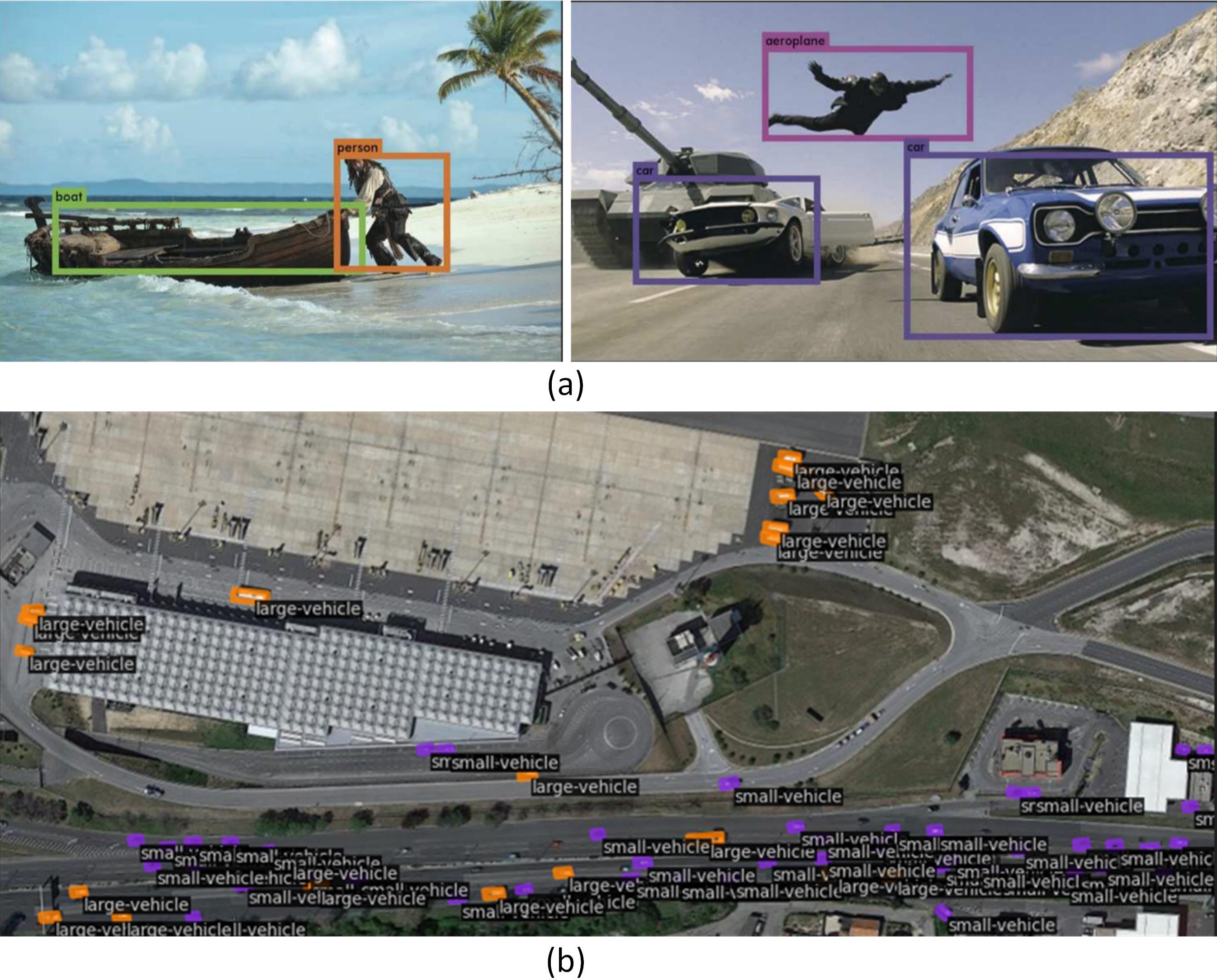
Figure 1: (a) Generic object detection: objects are usually sparsely distributed. (b) Aerial object detection: objects in remote sensing images are usually small, blurred, and densely distributed with complex backgrounds.

For the query type, existing solutions can be roughly divided into two categories, image-based (shown in Figure 2 (a)), and object-based (shown in Figure 2 (b)). Image-based AL methods estimate the uncertainty of the whole scene and require the bounding-box annotation of all objects in the scene [11, 12]. These approaches suffer from inefficient and redundant labeling problems as an aerial image usually contains many similar objects. Object-based AL methods [5, 6] query a specific object (i.e., bounding box) rather than the whole image for more fine-grained and cost-effective annotation. However, They only consider the uncertainty of the object but neglect the spatial information and the semantic structure of the image. On the other hand, they may introduce training noise as each image is partially annotated with particular objects, and the remaining regions are treated as background with remaining unlabeled objects, which would mislead the model training.

To address the problems above, in this paper, we present a novel active learning method for aerial object detection – Mixed Uncertainty Sampling with Class Distribution Balancing (MUS-CDB). For the query type, we propose an object-based mixed uncertainty sampling (MUS) method to label the most informative and representative objects. Unlike existing work, MUS addresses the limitations in object-based and image-based methods, i.e., the redundant and myopic information querying, by considering both object-level and image-level uncertain cues. For the query strategy, we propose a novel sample selection criteria with class distribution balancing (CDB), identifying the most helpful object samples to improve the performance of the current detection model while balancing the class distribution of training samples further to enhance the model’s capability on rare classes. We propose an effective training scheme associated with a loss function, which effectively mines the latent knowledge in the unlabeled regions that have not been queried as positive samples. Extensive experiments on DOTA-v1.0 [13] and DOTA-v2.0 [14] show that the proposed method can significantly outperform the conventional image- and object-based active learning methods for aerial object detection.

We summarize our contributions as the following:

1. We propose a novel active learning method for aerial object detection, which considers the characteristics of remote sensing data to actively select informative and representative object samples.

2. We propose a training scheme associated with a loss function for querying with partially labeled data. It robustly exploits the queried information from partial labels and effectively improves the model’s capability.

3. Extensive experiments on DOTA-v1.0 and DOTA-v2.0 validate the effectiveness and practicability of the proposed method for aerial object detection.

The rest of this paper is structured as follows. In Section II, we discuss the related work. In Section III, we introduce the proposed method in detail. The experimental results are presented in Section IV. Section V is the conclusion.

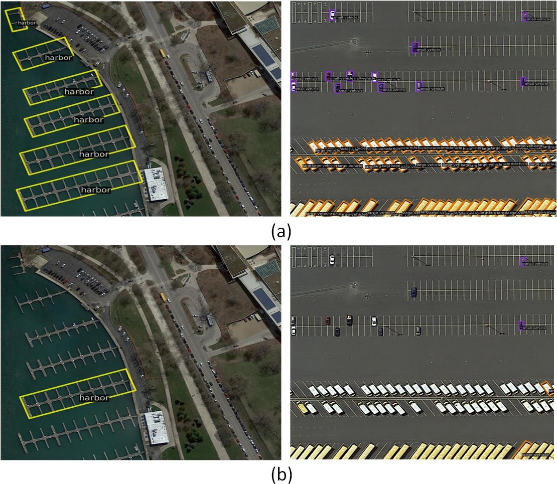
Figure 2: Illustration of different types of AL methods. (a) Image-based sampling annotates the whole image with inefficient and redundant annotation. (b) Object-based sampling selects objects that the model is most uncertain.

II RELATED WORK

II-A Aerial Object Detection

Compared with generic object detection, aerial object detection is more challenging. Many works have been proposed to solve the specific problems of aerial object detection.

Some methods use multiple anchors with different angles, scales, and aspect ratios for regressing the bounding boxes [15, 16]. However, these methods are usually computationally expensive. Another group of methods uses only horizontal anchors to detect rotated objects to improve efficiency. Ding et al. [17] propose an RoI Transformer to convert Horizontal RoIs (HRoIs) into RRoIs, which reduces the number of anchors. DRN [18] performs orientated object detection through dynamic feature selection and optimization. Wei et al. [19] propose a vision-transformer-based feature-calibrated guidance (CG) scheme to enhance feature channel communications. CSL [20] treats angle prediction as a classification task to avoid discontinuous boundary problems. ReDet [21] is committed to improving the model’s feature representation by modifying the backbone to generate rotation-equivariant features and employing RiRoI Align in the detection head to extract rotation-invariant features. Based on the popular Rotate-YOLO method, Sun et al. [22] introduced a bi-directional feature fusion module and an angle classification technique to a YOLO-based rotated ship detector.

For the challenge of small objects, many works address the challenge by designing networks that handle scale diversity. For instance, Qiu et al. [23] propose an adaptive aspect ratio network. It assigns different weights to the feature maps and predicts proper ratio aspects for different objects. Li et al. [24] design a perceptual generative adversarial network to enhance feature response, which converts the features of small targets into large ones with homogeneous attributes. Zheng et al. [25] propose a hyper-scale detector to learn scale-invariant representations of objects. Liang et al. [26] present a dynamic enhancement anchor network (DEA-Net) that contains a sample generator to augment the training data and a discriminator to distinguish the samples between an anchor-based unit and an anchor-free unit to help train the detector. Liu et al. [27] design an enhanced effective channel attention (EECA) mechanism, an adaptive feature pyramid network (AFPN), and a context enhancement module (CEM) in an adaptive balanced network (ABNet) to capture more discriminative features. Liu et al. [28] present a method to balance accuracy and speed by using a one-stage detector for high efficiency and design a balanced feature pyramid network (BFPN) that adaptively balances semantic and spatial information between high-level and low-level features. Most existing methods are based on the assumption that a large number of labeled data for model training is available. In fact, it is usually unavailable in real remote sensing applications due to the prohibitive cost of annotating large-scale remote sensing images with massive objects.

II-B Active Learning in Object Detection

The primary objective of active learning is to train a model with maximum accuracy while minimizing the number of labeled samples required for training [29]. This is achieved by selecting the most informative samples for labeling using various selection methods. It has been applied to many important tasks in computer vision, such as classification [30, 31, 32], detection [7, 33, 34] and segmentation [35, 36, 37].

Active learning mainly studies effective query strategies and query types. Many selection criteria are proposed for the former research topic to evaluate the informativeness of the unlabeled data from different aspects. Existing methods can mainly be divided into the uncertainty-based approaches [38, 39, 34, 7, 4], representativeness-based approaches [40, 30] and hybrid approaches [41, 42, 43, 44]. Uncertainty-based methods prefer the examples with high prediction uncertainty of the model. For example, Yoo et al. [34] add a loss prediction branch to the neural network to predict the loss of unlabeled samples. The data with large predicted loss will be queried from the oracle. Roy et al. [7] estimate the uncertainty by the difference between the convolutional layers of the object detector backbone. The data with high divergence are preferred in active selection. Kao et al. [4] propose “localization tightness” and “localization stability” criteria. They measure the overlap ratio between region proposals and final predictions and the prediction changes of the original and corrupted images to evaluate the uncertainty. Representativeness-based methods prefer data that can represent the latent data distribution. Sener et al. [40] propose a Coreset method to query the data that can cover the whole dataset with a minimum radius. Sinha et al. [30] train a variational autoencoder (VAE) and an adversarial network to classify the unlabeled and labeled data, then select the predicted data from the unlabeled one. For the hybrid methods, Ash et al. [43] cluster the gradient of the target model’s final output layer as the feature of the unlabeled samples that contain the uncertainty information. Sharat et al. [44] use the probability vector predicted by CNN to select objects located in different backgrounds.

For the query type, many methods are proposed to improve the querying efficiency by an effective query type, i.e., taking an object rather than the image as the basic unit for querying [45, 5, 6]. For example, Tang et al. [5] consider the partial transfer object detection task and query the source objects which are informative and transferrable to the target domain. Laielli et al. [46] propose a region-level sampling method, which calculates the score of each region according to an accumulation of the informativeness and similarity of each query-neighbor pairing within a region and finally selects the image region with the highest score to send to the experts for annotation. Xie et al. [47] propose a region-based active learning approach for semantic segmentation with domain shift. The authors evaluate the informativeness by the category diversity of pixels within a region and the classification uncertainty. Liang et al. [48] propose a sampling method combining spatial and temporal diversity to label the most informative frames and objects in multimodal data.

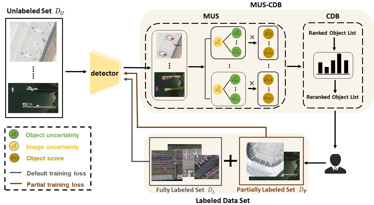
Figure 3: Overall framework of the proposed method. The overall framework of the proposed method consists of two modules: Mixed Uncertainty Sampling (MUS) and Class Distribution Balancing (CDB), which together form the active learning sampling strategy. The MUS module combines image uncertainty and object uncertainty to obtain the final object information. The CDB module performs class-balanced sampling on the objects selected by MUS based on the prior distribution of labeled objects in the pool. We take the model prediction object as the basic sampling unit and send it to experts for labeling.

III The Methodology

III-A Problem Definition

The problem definition for remote sensing object detection using active learning is to reduce the labeling cost by selecting informative samples from a large unlabeled dataset $\mathcal{D}_{U}$ to train a well-performing detector $f$. The problem is defined by three sets of data: a small fully labeled set $\mathcal{D}_{L}$ used to initialize the model, a large unlabeled set $\mathcal{D}_{U}$ used for data selection, and a partially labeled set $\mathcal{D}_{P}$ updated with informative queries selected by an active learning method. $\mathcal{D}_{L}$ is expressed as

$$\mathcal{D}_{L}=\{(X_{i}^{L},\mathcal{Y}_{i}^{L})\}_{i=1}^{N_{L}},$$ (1)

where $X_{i}^{L}$ represents the $i^{\operatorname{th}}$ image in the fully labeled set $\mathcal{D}_{L}$, and $\mathcal{Y}_{i}^{L}=\{(\textbf{c}_{ij}^{L},\textbf{b}_{ij}^{L})\}_{j=1}^{n_{i}}$ with $\textbf{c}_{ij}^{L}$ being the one-hot class label belonging to one of the $C$ known classes in label space and $\textbf{b}_{ij}^{L}$ being the bounding box label. In summary, $\mathcal{D}_{L}$ is a set of $N_{L}$ images, each annotated with one or more ground truth bounding boxes, where each bounding box is associated with a one-hot class label. $\mathcal{D}_{U}$ is expressed as

$$\mathcal{D}_{U}=\{(X_{i}^{U})\}_{i=1}^{N_{U}}$$ (2)

where $N_{U}\gg N_{L}$, and $\mathcal{P}_{U}$ is the model prediction on the unlabeled set $\mathcal{D}_{U}$, expressed as

$$\mathcal{P}_{U}=\{(X_{i}^{U},\mathcal{\hat{Y}}_{i}^{U})\}_{i=1}^{N_{U}}$$ (3)

where $\mathcal{\hat{Y}}_{i}^{U}=\{(\mathbf{\hat{c}}_{ij}^{U},\mathbf{\hat{b}}_{ij}^{U})\}_{j=1}^{\hat{n}_{i}}$ denotes the model’s prediction. Specifically, $\mathcal{\hat{Y}}_{i}^{U}$ consists of two parts, $\mathbf{\hat{c}}_{ij}^{U}$ is the predicted class probability vector from the classification head where $\mathbf{\hat{c}}_{ij}^{U}=\{\hat{c}_{ijk}^{U}\}_{k=1}^{C}$, and $\mathbf{\hat{b}}_{ij}^{U}$ is the predicted bounding box position from the regression head.

To train a well-performing detector $f$ with minimal labeling effort from $\mathcal{D}_{U}$, a sampling function ($\varphi$) is employed to select informative samples from the unlabeled image set $\mathcal{D}_{U}$. Specifically, the sampling function $\varphi$ takes $\mathcal{P}_{U}$ as input to select the informative data for labeling. For the proposed object-based active learning method, we evaluate each predicted bounding box in $\mathcal{P}_{U}$ and select the top $N$ most informative bounding boxes for labeling. Once labeled, these bounding boxes are added to the partially labeled set

$$\mathcal{D}_{P}=\{(X_{i}^{P},\mathcal{Y}_{i}^{P})\}_{i=1}^{N_{P}}$$ (4)

to improve the object detector $f$.

In this work, we design two modules to perform a cost-effective selection for objects, i.e., the object-based mixed uncertainty sampling module (MUS) and the class distribution balancing module (CDB). The overall framework of the method is shown in Figure 3. Next, we will introduce the proposed method in detail and elaborate on the training scheme to fully utilize the partial labels.

III-B Mixed Uncertainty Sampling

As aforementioned, existing object-based sampling methods mainly consider the information of the prediction box itself, i.e., category uncertainty or regression uncertainty, but neglect the spatial information and the semantic structure of the image. To tackle this problem, we propose to consider both uncertainty of the image and the object for more comprehensive data evaluation, which incorporates both global and local information.

As for the image uncertainty, if there are many predicted objects with high uncertainty in an image, this image should be preferred to be selected as a labeling candidate. To this end, we evaluate and aggregate the uncertainty values with the most confident model predictions (i.e., objects whose predicted class confidence is greater than a specific threshold) to indicate the uncertainty value of the whole image. Specifically, the image uncertainty $\varphi_{i}^{I}$ for a given image $X_{i}^{U}$ is formulated as

$$\varphi_{i}^{I}=1-\frac{1}{|\mathcal{S}^{\theta}_{i}|}\sum_{j\in\mathcal{S}^{\theta}_{i}}\max\mathbf{\hat{c}}_{ij}^{U}\,,$$ (5)

where $\mathcal{S}^{\theta}_{i}=\{j|\max\mathbf{\hat{c}}_{ij}^{U}>\theta,\forall j=1,\dots,\hat{n}_{i}\}$ , and $|\cdot|$ represents the number of elements in the set and $\theta$ is the threshold. The image uncertainty value $\varphi_{i}^{I}$ is calculated as the difference between 1 and the average confidence score of the predicted bounding boxes. Only predicted bounding boxes with class confidence scores greater than the threshold $\theta$ are used to calculate the average confidence score. The set ${S}^{\theta}_{i}$ represents the indices of the predicted bounding boxes in an image $i$ whose maximum class confidence score is greater than the threshold $\theta$. The value of $\varphi_{i}^{I}$ is high when an image has many predicted bounding boxes with low confidence scores, which may occur when an image contains many objects that are difficult to distinguish, resulting in inconsistent and low-confidence predictions. Therefore images with higher values of $\varphi_{i}^{I}$ are more likely to contain informative knowledge of rare patterns, making them more suitable for selection.

To consider the object-level information in the querying, we employ entropy to evaluate the uncertainty of each predicted bounding box. Specifically, the object uncertainty $\varphi_{ij}^{O}$ is calculated as follows

$$\varphi_{ij}^{O}=-\sum_{k=1}^{C}\mathbb{P}(\hat{c}_{ijk}^{U}|X_{i}^{U})\log\mathbb{P}(\hat{c}_{ijk}^{U}|X_{i}^{U})\,,$$ (6)

where $\mathbb{P}(\hat{c}_{ijk}^{U}|X_{i}^{U})$ is the predicted probability of the $j^{\operatorname{th}}$ bounding box in the image $X_{i}^{U}$ on class $k$.

Next, we combine the image uncertainty $\varphi_{i}^{I}$ and object uncertainty $\varphi_{ij}^{O}$ to obtain the final object information score $\varphi_{ij}$, as shown in Equ. (7).

$$\varphi_{ij}=\varphi_{i}^{I}\cdot\varphi_{ij}^{O}\,,$$ (7)

$$\forall i=1, \dots,N^{U},\;\forall j=1,\dots,\hat{n}_{i}\,.$$

III-C Class Distribution Balancing

Remote sensing data suffer from the problem of class imbalance [13], as some categories are naturally rare. This phenomenon will significantly jeopardize the model performance, especially for the rare categories. To tackle this problem, we propose a criterion emphasizing the categories with low occurrence frequency in active querying. The process of class distribution balancing is shown in Figure 4. Specifically, we first identify the rare categories by counting the objects of each class on the labeled set, which is a combination of the initial fully labeled set $\mathcal{D}_{L}$ and the partially labeled set $\mathcal{D}_{P}$. Let $a_{k}$ denote the number of objects in class $k$, $\forall k=1,\dots,C$. We aim to query more objects in classes with fewer objects by imposing a preference $\zeta_{k}$, which is inversely proportional to $a_{k}$, on each class during the selection phase. Specifically, we calculate the preference value $\zeta_{k}$ as follows:

$$\zeta_{k}=\frac{exp(\beta_{k})}{\sum\limits_{k}exp(\beta_{k})}$$ (8)

where

$$\beta_{k}=1-\frac{a_{k}}{\sum\limits_{k}a_{k}}\,.$$ (9)

we first calculate the distribution probability of each class in the labeled set based on $a_{k}$, then take the inverse to obtain the class weight $\beta_{k}$ during sampling. We then use the softmax function, as shown in Equ. (8), to compute the expected class distribution during sampling. This allows us to set preferences for different classes and selectively query objects in classes with fewer objects during the selection phase, thereby improving the performance and accuracy of the model.

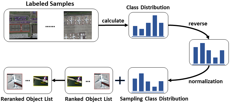
Figure 4: The proposed Class Distribution Balancing module (CDB) procedure. We reverse the class distribution of the labeled samples and perform a softmax operation to obtain the distribution that the class should satisfy when sampling.

III-D Two-Stage Sampling

We summarize our active learning method in Figure 3 and Algorithm1, which aims to select high-information objects for annotation while optimizing the labeling budget and improving the model’s performance. The method includes mixed uncertainty sampling (MUS) and Class Distribution Balancing (CDB) stages. In the MUS stage, as described in Figure 3, we take the unlabeled images from the $\mathcal{D}_{U}$ and feed them into a pre-trained object detector to obtain the model prediction. We then calculate the uncertainty value of each predicted object using Equ. (6) and the uncertainty value of each image using Equ. (5) based on the model’s output class probability vector $\mathbf{\hat{c}}_{ij}^{U}$. Finally, we calculate the information value of each predicted object using Equ. (7). In the CDB stage, we allocate the labeling budget for each class based on the corresponding class preference value $\zeta_{k}$. Specifically, we determine the labeling budget for each class by multiplying the total labeling budget by the class preference value. Then, During the sampling phase, we select high-value objects for annotation based on a balanced class distribution strategy. Specifically, we select enough objects from each class based on their information value in descending order and the labeling budget determined in the previous step. If the labeling budget for a specific class has been exhausted, we discard any remaining objects predicted as belonging to that class. Using this approach, we can effectively select high-information objects for annotation while optimizing the labeling budget and improving the model’s performance.

III-E Dealing with Partially Labeled Data

To deal with the situations where some samples are fully labeled while others are only partially labeled during the model training, we use different training losses for the two sets. For the fully labeled dataset, we use the default training loss of the specific detector; For the partially labeled dataset, we use a loss function to effectively mine the latent knowledge in the unlabeled image regions that have not been queried. Since some objects in the partially labeled images are not labeled, training the model with these images can mislead the model’s classification head. To address this issue, we propose an adaptive weight loss function that uses the predicted box background score as the weight for each negative box’s classification loss. Specifically, in object detection models ([21, 49, 50, 51] ), the bounding-box head loss $\mathcal{L}_{bbox}$ is a key component comprising both classification and regression losses. The classification loss $\mathcal{L}_{cls}$ measures the accuracy of object classification, including positive and negative sample losses, while the regression loss $\mathcal{L}_{reg}$ measures the accuracy of the predicted bounding box location, consisting only of positive sample losses. However, training the model with partially labeled images can introduce noise to the negative sample losses in the classification loss since some objects in the images may not be labeled and are treated as negative samples. To address this issue, we propose an adaptive weight loss function for the negative sample losses in the classification loss. Specifically, we add an adaptive weight to each negative sample’s classification loss based on the predicted background score of the sample. This method can effectively suppress the classification loss of negative samples with low background scores, which the model considers foreground objects. Formally, the $\mathcal{L}_{bbox}$ is defined as follows

$$\mathcal{L}_{bbox}= \mathcal{L}_{cls}+\mathcal{L}_{reg}$$ (10)

$$=(\lambda_{cls}\sum_{j=1}^{W}\sum_{k=1}^{C+1}\mathbb{I}_{i}^{partially}\omega[-\mathbf{{o}_{ijk}}\log(\mathbf{\hat{o}_{ijk}})]+$$

$$\lambda_{cls}\sum_{j=1}^{W}\sum_{k=1}^{C+1}\mathbb{I}_{i}^{fully}[-\mathbf{{o}_{ijk}}\log(\mathbf{\hat{o}_{ijk}})])$$

$$+\lambda_{reg}\sum_{j=1}^{W}\sum_{u=1}^{5}\mathbb{I}_{ij}^{obj}\ell_{s}(\hat{v}_{iju}-v_{iju})\,,$$

where

$$\omega=\left\{\begin{aligned} 1\quad\mathbb{I}_{ij}^{obj}=1\\ \mu\quad\mathbb{I}_{ij}^{obj}=0\end{aligned}\right.$$ (11)

and

$$\ell_{s}(x)=\begin{cases}0.5(x)^{2},\quad&if|x|<1\\ |x|-0.5,\quad&otherwise\end{cases}.$$ (12)

Here $i$ and $j$ are the images and region proposals indexes in a mini-batch, respectively. $W$ indicates the number of proposals involved in bounding-box heads in training. $\mathbb{I}_{i}^{partially}$ and $\mathbb{I}_{i}^{fully}$ are indicator functions. When an image $i$ is partially labeled, $\mathbb{I}_{i}^{partially}$ equals 1 and $\mathbb{I}_{i}^{fully}$ equals 0. When an image $i$ is fully labeled, $\mathbb{I}_{i}^{partially}$ equals 0 and $\mathbb{I}_{i}^{fully}$ equals 1. $\mathbb{I}_{ij}^{obj}$ indicates whether the proposal contains a foreground object. $\omega$ is introduced to down-weighting the background objects for robust learning. The classification and regression losses are normalized using the balancing parameters $\lambda_{cls}$ and $\lambda_{reg}$, respectively [52]. Specifically, the number of proposals in a mini-batch is used to normalize the classification loss, while the number of positive proposals in the mini-batch is used to normalize the regression loss.

The $\mathcal{L}_{bbox}$ contains the classification loss (the first two terms) and the box regression loss (the last term). For the classification loss, the model predicts a discrete probability distribution over $C$ categories plus the background for each proposal, i.e., $\mathbf{\hat{o}_{ijk}},\forall k=1,\dots,C+1$. The regression loss is defined over the bounding-box coordinate offsets plus the angle, i.e., $\hat{v}_{iju},\,\forall u=1,\dots,5$. Further, the smooth L1 regularization $\ell_{s}$ is employed to stabilize the training.

Algorithm 1 Our proposed MUS-CDB

1:initial labeled set $D_{L}$, unlabeled set $D_{U}$, partailly labeled set $D_{P}$, annotation budget $N$, detection model $f$.

2:Train the detection model $f$ with $D_{L}$.

3:$\mathcal{P}^{U}\leftarrow\{(X_{i}^{U},f(X_{i}^{U})\,|\,\forall i=1,...,N_{U}\}$.

4:Remove the objects in $\mathcal{P}^{U}$, which highly overlap with the labeled object.

5:$\mathbf{\zeta}\leftarrow\{\zeta_{k}\,|\,\forall k=1,\dots,C\}$. $\triangleright$ by Equ. (8)

6:$\Phi\leftarrow\{\varphi_{ij}\,|\,\forall i=1,\dots,N^{U},\;\forall j=1,\dots,\hat{n}_{i}\}$. $\triangleright$ By Equ. (7)

7:$\mathbf{a}\leftarrow\{a_{k}\,|\,a_{k}=N\cdot\zeta_{k},\,\forall k=1,\dots,C\}$. $\triangleright$ calculate the labeling budget for each class

8:$\Phi\leftarrow\operatorname{sort}(\Phi)$. $\triangleright$ sort $\Phi$ in descending order

9:while $N>0$ do

10:     $i,j\leftarrow\{i,j\,|\,\varphi_{ij}=\operatorname{pop}(\Phi)\}$.

11:     $c\leftarrow\text{argmax}\{\hat{\mathbf{c}}_{ij}^{U}\}$.

12:     if $a_{c}>0$ then

13:         $D_{P}\leftarrow D_{P}\cup\operatorname{label}(\varphi_{ij})$. $\triangleright$ label the $\varphi_{ij}$ instance according to the labeling rule

14:         $a_{c}\leftarrow a_{c}-1$.

15:         $N\leftarrow N-1$.

16:     end if

17:end while

18:the updated queried set $D_{P}$

IV Experiments

IV-A Experimental Settings

IV-A1 Dataset

DOTA is a popular object detection dataset in aerial imagery. We conduct experiments on DOTA-v1.0 [13] and DOTA-v2.0 [14]. Specifically, DOTA-v1.0 contains 2,806 large-scale aerial images and 188,282 objects. DOTA-v2.0 collects more Google Earth, GF-2 Satellite, and aerial images. There are 11,268 images and 1,793,658 objects in DOTA-v2.0. Each image is between 800 $\times$ 800 and 20000 $\times$ 20000 pixels in size. There are a total of 15 classes in the DOTA-v1.0 [containing plane] (PL), [baseball diamond] (BD), [bridge] (BR), [ground track field] (GTF), [small vehicle] (SV), [large vehicle] (LV), [ship] (SH), [tennis court] (TC), [basketball court] (BC), [storage tank] (ST), [soccer-ball field] (SBF), [roundabout] (RA), [harbor] (HA), [swimming pool] (SP) and [helicopter] (HC). DOTA-v2.0 further adds the new categories: [container crane] (CC), [airport] (AP), and [helipad] (HP).

For DOTA-v1.0, the training and testing sets follow the setup of the previous work [21]. For DOTA-v2.0, since the server for uploading the results is unstable, we use the training set for training and the validation set for testing. We crop the original image to 1024 $\times$ 1024 patches with an overlap of 200. The random horizontal flip is employed in data augmentation.

IV-A2 Comparison AL Methods

We compare the proposed method with various types of active learning methods, including random selection (Random), uncertainty-based active learning methods (Entropy [29]), representation-based active learning methods (Coreset [40]), detection-specific active learning methods (Localization Stability [4]) and object-level active learning methods (Qbox [5], BiB [53] and TALISMAN [54]. Both Qbox [5] and our proposed method utilize an object-based query approach to select informative samples for annotation. In contrast, other methods employ an image-based query approach. In Qbox [5], we use the model-predicted bounding boxes as candidate objects for sampling and calculate their informativeness using the inconsistency metric defined in Qbox [5]. The predicted bounding boxes are then sent to the oracle for labeling in descending order of informativeness. Meanwhile, for image-based methods such as entropy [29], we calculate the entropy of each object using the model-predicted class probabilities and then average them to obtain an information score for the image. For TALISMAN, we set the sampling quantity for rare classes in DOTA-v1.0 and DOTA-v2.0 to 2 in the query set.

IV-A3 Labeling Rules

Image-based and object-based AL methods have different labeling rules. Object-based AL methods send the predicted bounding box as a unit to the oracle for labeling. If there is only one unlabeled ground-truth object in the query bounding box, the label of that object is returned. If multiple unlabeled ground-truth objects exist in the query bounding box, calculate the IoU of each ground-truth object and the query bounding box, and return the object’s label with the largest IoU. After the queried bounding box obtains the object annotations, the annotation cost (i.e., the number of annotated objects) is increased by one.

IV-A4 The detectors

The active learning experiments were conducted using the ReDet [21] architecture with ReResNet50 pretrained on ImageNet [55] as the baseline detector on the DOTA-v1.0 and DOTA-v2.0 datasets. To further validate the generality and effectiveness of our proposed method MUS-CDB, we conducted experiments on other two single-stage remote sensing object detectors KLD [50], SASM [51] and one other two-stage remote sensing object detectors Oriented R-CNN [49].

IV-A5 Dataset Partitioning

Regarding the dataset partitioning, for DOTA-v1.0, We randomly select 5% images (1052 images) from the training and validation sets as the initially fully labeled set, with the remaining images making up the unlabeled set. In each round of active learning, 5000 objects are selected from the unlabeled set for querying. These objects are then labeled (we use the ground truth in the experiments) and added to the partially labeled set for fine-tuning the detector. This process is repeated for multiple rounds until the budget for annotation is exhausted. For DOTA-v2.0, we randomly selected 500 images from the training set as the initially fully labeled set, with the remaining images being considered the unlabeled set. In each round, 1000 objects are selected from the unlabeled set for querying. The model was fine-tuned on the labeled set (combination of fully labeled set and partially labeled set) for a fixed number of epochs in each round of active learning.

IV-A6 Training Settings

For ReDet, the model with default pre-trained weights will be fine-tuned on the labeled set for 12 epochs with a batch size of 2, and the initial learning rate is set to 2.5 $\times$ $10^{-3}$, using the SGD optimizer mentum of 0.9 and weight decay of 1 $\times$ $10^{-4}$. The learning rate is reduced by 0.1 at 8 and 11 epochs. On the DOTA-v1.0 dataset, the loss value of the model decreased from an initial value of 1.076 to a final value of 0.656, and the entire loss curve showed a downward trend. Similarly, on the DOTA v2.0 dataset, the loss value of the model decreased from an initial value of 1.694 to a final value of 0.8551, and the entire loss curve showed a downward trend. For the other two-stage detector Oriented R-CNN [49], we set the initial learning rate to 5 $\times$ $10^{-4}$ and keep other variables consistent with ReDet’s settings. For KLD [50], we trained the model for 14 epochs with a batch size of 2. The initial learning rate was set to 1 $\times$ $10^{-3}$, and the settings for the SGD optimizer were fixed. The learning rate was reduced by 0.1 at 10 and 13 epochs. Similarly, for SASM [51], we used the same training strategy as KLD [50], including the same number of epochs, batch size, learning rate, optimizer, and weight decay.

IV-A7 Other Settings

For active learning, the parameter settings involved in our sampling method are as follows. We implement the adaptive weight $\mu$ in Equ. (11) as the background score predicted by the model for proposals. In this way, we can reduce the impact of the partially labeled data by down-weighting the loss of the false-negative objects, which typically have lower background scores than background regions. Regarding the hyperparameter $\theta$ in Equ. 5, we set it to 0.10, and Table IV lists the performance change of our method under different values of this parameter. All experiments are conducted on 4 NVIDIA GeForce GTX 2080Ti GPUs.

TABLE I: Comparison of mAP(%) for ReDet [21], Oriented R-CNN [49], KLD [50] and SASM [51] using different AL methods on DOTA-v1.0 [13] and DOTA-v2.0 [14] with different numbers of Cycles. Numbers in bold are the best results per column. * denotes the AL method that follows the object-based query type. The Cycle-0 column reports the detector’s performance without active learning sampling.

Detector	ReDet [21]										Oriented R-CNN[49]
Dataset	DOTA-v1.0 [13]					DOTA-V2.0 [14]					DOTA-v2.0 [13]
AL cycle	Cycle-0	Cycle-1	Cycle-2	Cycle-3	Cycle-4	Cycle-0	Cycle-1	Cycle-2	Cycle-3	Cycle-4	Cycle-0	Cycle-1	Cycle-2	Cycle-3	Cycle-4
Random	53.9	58.1	60.3	61.8	64.4	22.8	24.6	25.1	25.3	26.2	6.3	6.3	9.2	10.1	10.4
Coreset [40]	53.9	55.8	59.6	62.1	63.6	22.8	23.5	23.8	25.1	26.6	6.3	7.5	10.2	11.5	13.0
Localization Stability [4]	53.9	61.6	63.7	66.8	66.9	22.8	27.1	30.9	31.1	33.5	6.3	13.9	16.9	16.0	17.1
Entropy [4]	53.9	64.2	65.7	67.2	67.4	22.8	28.3	30.9	31.7	35.0	6.3	14.8	20.1	22.0	24.8
Qbox∗ [5]	53.9	58.7	61.4	64.1	65.2	22.8	24.1	27.8	28.8	31.2	6.3	14.7	17.1	18.7	20.4
BiB [53]	53.9	60.9	65.0	66.4	66.8	22.8	23.7	24.4	26.6	28.2	6.3	11.6	16.3	18.6	19.9
TALISMAN-FLMI [54]	53.9	58.9	60.7	61.0	62.0	22.8	25.6	31.4	33.0	36.6	6.3	13.0	17.3	19.1	20.0
TALISMAN-GCMI [54]	53.9	59.9	61.3	63.5	65.4	22.8	30.4	32.9	38.4	40.0	6.3	13.8	17.3	19.8	20.9
MUS∗	53.9	64.6	66.3	68.3	69.1	22.8	33.0	35.8	38.0	39.5	6.3	15.9	20.7	24.7	28.2
CDB∗	53.9	65.2	66.9	69.2	69.2	22.8	33.2	36.1	39.1	40.6	6.3	16.7	22.9	25.9	28.4
MUS-CDB∗	53.9	64.9	67.3	69.2	70.1	22.8	34.1	37.2	40.2	40.9	6.3	17.3	22.7	26.0	28.2

Detector	KLD [50]					SASM [51]
Dataset	DOTA-v2.0 [13]
AL cycle	Cycle-0	Cycle-1	Cycle-2	Cycle-3	Cycle-4	Cycle-0	Cycle-1	Cycle-2	Cycle-3	Cycle-4
Random	1.9	2.1	3.3	2.9	3.7	11.7	13.3	11.8	14.1	16.2
Coreset [40]	1.9	1.1	2.2	2.4	2.2	11.7	12.2	11.2	13.6	11.1
Localization Stability [4]	1.9	2.2	2.7	3.9	3.5	11.7	13.6	18.2	19.3	20.9
Entropy [29]	1.9	2.1	4.7	5.5	8.6	11.7	13.8	14.4	14.6	15.3
MUS-CDB∗	1.9	9.8	13.4	16.8	21.7	11.7	18.6	24.8	28.0	30.0

IV-B Performance Comparison

IV-B1 AL Performance Comparisons with Different Detectors

We report the performances of all AL methods on the DOTA-v1.0 and DOTA-v2.0 benchmarks to demonstrate that our method can better mine the most informative objects from the unlabeled data pool in remote sensing scenarios. The experimental results of the two datasets are shown in Table I.

For ReDet, we conducted experiments on both DOTA-v1.0 and DOTA-v2.0 datasets. For DOTA-v1.0 in Table I, MUS-CDB significantly outperforms the other methods at each active learning cycle. Specifically, in terms of mAP, when 5000, 10000, 15000, and 20000 objects were sampled, the MUS-CDB surpassed the random method by 6.8, 7, 7.4, and 5.7, and the sub-optimal method by 0.7, 1.6, 2 and 2.7, respectively. For DOTA-v2.0, MUS-CDB shows more impressive improvements over image-based and object-based sampling methods. The results in Table I demonstrate that in terms of mAP, when 1000, 2000, 3000, and 4000 objects are sampled, the MUS-CDB surpassed the random method by 9.5, 12.1, 14.9, and 14.7, and the sub-optimal method by 3.7, 4.3, 1.8 and 0.9, respectively. The performance improvement on DOTA-v2.0 is more significant than that on DOTA-v1.0, which shows our approach can better guide low-performing models to sample highly informative objects based on only a small number of training samples. Furthermore, Table I demonstrates that our method achieves comparable or even better performance than other methods that sample 4000 unlabeled objects (Cycle-4) in DOTA-v2.0 by only querying 1000 unlabeled objects (Cycle-0), except for TALISMAN-gcmi. For the ReDet, KLD and SASM detector on the DOTA-v2.0 dataset, the results show that our proposed MUS-CDB method can save nearly 75% of the labeling cost while achieving comparable performance to other active learning methods in terms of mAP.

Based on the results presented in Table I, it is evident that Entropy and Localization Stability perform well in both DOTA-v1.0 and DOTA-v2.0 datasets. Conversely, Coreset and Random perform poorly, as expected. This finding highlights that uncertainty-based methods are more effective than representativeness-based ones in dealing with chaotic scenes. Moreover, the object-based sampling method Qbox performs poorly on either dataset. Qbox was designed for generic scenes, which differ from remote-sensing scenes. The sampling strategy of Qbox cannot accurately identify the informativeness of objects in remote-sensing images. Talisman performs well on the DOTA-v2.0 dataset. However, its performance on the DOTA-v1.0 dataset is relatively poor, and there is also a significant performance gap between Talisman and our method in the early rounds of the DOTA-v2.0 dataset. On the other hand, it is worth noting that the BiB method did not perform well on either dataset, especially in the early rounds, where its performance was even worse than that of Random. This may be caused by the fact that BiB was designed for weakly supervised object detection tasks and could not effectively leverage fully supervised knowledge.

TABLE II: Comparison of AP (%) for ReDet [21] using different AL methods on DOTA-v2.0 [14] validation set after 5 cycles of active learning. The optimal and second optimal results in each column are highlighted in bold, and the second optimal results are underlined to distinguish them. * denotes that the AL method follows the object-based query type.

	Common			Middle						Rare
category	SH	SV	LV	PL	HA	ST	TC	BR	SP	HC	BC	BD	RA	SBF	GTF	CC	AP
Random	59.2	29.5	37.5	72.5	11.7	47.5	74.4	2.4	23.5	0.0	5.0	18.3	35.3	8.3	19.2	0.0	2.1
Coreset [40]	63.3	29.1	36.3	71.9	17.8	47.9	74.4	3.9	20.4	0.0	2.2	8.5	38.2	9.1	15.5	0.0	0.0
Localization Stability [4]	59.2	28.8	33.3	76.9	13.2	48.8	75.8	20.0	21.2	4.3	16.2	33.6	41.5	13.3	29.7	0.0	7.5
Entropy [29]	58.7	29.6	37.3	75.6	8.9	47.9	78.6	6.2	20.8	24.0	28.1	36.9	37.5	12.7	29.9	0.0	2.6
Qbox∗ [5]	64.6	31.7	44.3	70.9	9.1	47.9	77.9	3.4	22.3	0.0	14.0	17.2	37.9	11.8	32.2	0.0	0.1
BiB [53]	58.3	29.8	36.2	75.2	7.5	47.5	79.9	2.3	18.5	0.0	11.1	24.2	35.1	8.9	18.2	0.0	0.0
TALISMAN-FLMI [54]	59.9	30.8	36.3	76.7	14.7	48.0	79.2	7.5	23.9	0.1	29.1	28.7	41.2	26.4	31.5	0.0	3.8
TALISMAN-GCMI [54]	58.4	29.3	33.9	77.7	10.2	52.3	74.9	19.5	22.2	5.3	16.8	47.6	49.3	24.6	44.4	0.0	25.7
MUS∗	63.3	30.6	41.3	73.8	15.2	48.6	79.2	7.4	25.8	3.6	37.1	42.4	45.3	34.5	50.2	0.3	10.3
CDB∗	63.0	30.2	41.4	75.3	17.7	49.1	81.4	9.6	25.8	8.1	42.2	45.2	42.5	31.2	49.3	0.0	6.9
MUS-CDB∗	64.0	30.8	40.9	74.9	16.3	49.0	81.2	11.9	25.5	6.9	41.6	43.9	45.2	32.8	52.5	0.04	13.5

TABLE III: Comparison of AP (%) for ReDet [21] using different AL methods on DOTA-v1.0 [14] test set after 5 cycles of active learning. The optimal and second optimal results in each column are highlighted in bold, and the second optimal results are underlined to distinguish them. * denotes that the AL method follows the object-based query type.

	Common			Middle						Rare
category	SH	SV	LV	PL	HA	ST	TC	BR	SP	HC	BC	BD	RA	SBF	GTF
Random	78.9	72.0	68.4	88.3	54.6	76.8	90.8	35.0	56.0	10.6	68.9	58.3	54.6	38.0	49.9
Coreset [40]	81.0	71.5	66.1	88.1	54.2	75.3	90.8	31.8	51.2	24.6	65.6	52.5	51.1	33.7	47.5
Localization Stability [4]	77.9	72.0	68.0	88.8	48.4	76.3	90.8	42.4	54.1	23.0	73.9	66.6	55.3	41.6	59.8
Entropy [29]	77.7	70.7	67.2	88.6	45.6	74.5	90.9	32.5	53.4	37.6	76.7	71.5	54.9	50.5	62.9
Qbox∗ [5]	78.1	72.0	69.5	87.7	46.6	74.6	90.7	32.3	52.9	23.3	67.6	63.2	50.7	42.8	58.1
BiB [53]	78.0	71.1	65.2	88.4	54.9	77.5	90.8	39.2	53.7	22.5	72.6	69.7	54.0	46.7	54.9
TALISMAN-FLMI [54]	78.0	71.5	67.1	88.9	47.6	78.6	90.7	35.5	51.9	15.0	68.2	58.7	52.3	35.1	50.4
TALISMAN-GCMI [54]	78.2	71.2	66.0	88.8	50.4	78.7	90.7	35.6	55.5	21.3	69.1	61.7	52.6	37.7	54.7
MUS∗	81.1	71.7	69.6	88.3	53.1	77.4	90.7	37.2	54.9	32.8	72.4	68.9	55.7	50.9	62.1
CDB∗	79.5	71.6	69.2	88.5	54.0	78.2	90.7	36.8	59.1	33.2	72.1	69.4	57.4	50.7	62.6
MUS-CDB∗	79.5	71.7	69.2	88.8	53.3	78.5	90.7	38.8	57.3	33.1	73.9	70.8	55.9	51.2	63.4

For the detectors KLD [50] and SASM [51], the experiments were conducted on DOTA-v2.0 [14] validation set, and we compared the proposed method with four other commonly used active learning methods, including random, Coreset, Localization Stability, and entropy. We did not compare our method with the Qbox, BiB, and Talisman methods on the KLD [50] and SASM [51] detectors. This is because single-stage detectors do not output background scores and prediction box features necessary for calculating sample information using the Qbox, BiB, and Talisman methods. The experimental results are presented in Table I. The proposed method significantly improved both KLD [50] and SASM [51] detectors, demonstrating the generality and effectiveness of the proposed approach on different types of detectors.

Regarding the two-stage detector Oriented R-CNN [49], we evaluated its performance using different AL methods on the DOTA-v2.0 validation set, and the mAP values are presented in Table I.

In summary, our experiments on multiple detectors demonstrate the effectiveness and generalizability of the proposed method MUS-CDB. The proposed approach can be easily integrated into various object detection frameworks and can help improve the performance of object detection models in various applications.

IV-B2 Category-wise AP

Table II and III show the average category-wise AP of all the compared methods using ReDet detector, on DOTA-v1.0 and DOTA-v2.0, respectively. From Table II and III, we can observe that MUS-CDB and its variants can usually achieve the best performance in most categories.

Qbox and uncertainty-based active learning methods tend to excessively query specific categories while ignoring the overall performance improvement. For example, Qbox focuses on improving the performance of [bridge], [tennis court], and [storage tank] but neglects the performance improvement of rare categories. Similarly, entropy-based methods only improve performance for a few middle and rare categories, such as [helicopter] and [container crane], while paying little attention to other categories, such as [plane], [swimming pool], and [ground track field]. Furthermore, it is worth noting that BiB could not accurately query rare categories for annotation, while TALISMAN-GCMI could only find and annotate a limited number of rare categories. In contrast, our method can effectively improve the performance of all categories, including rare categories. This highlights the effectiveness and versatility of our proposed method for remote sensing object detection tasks.

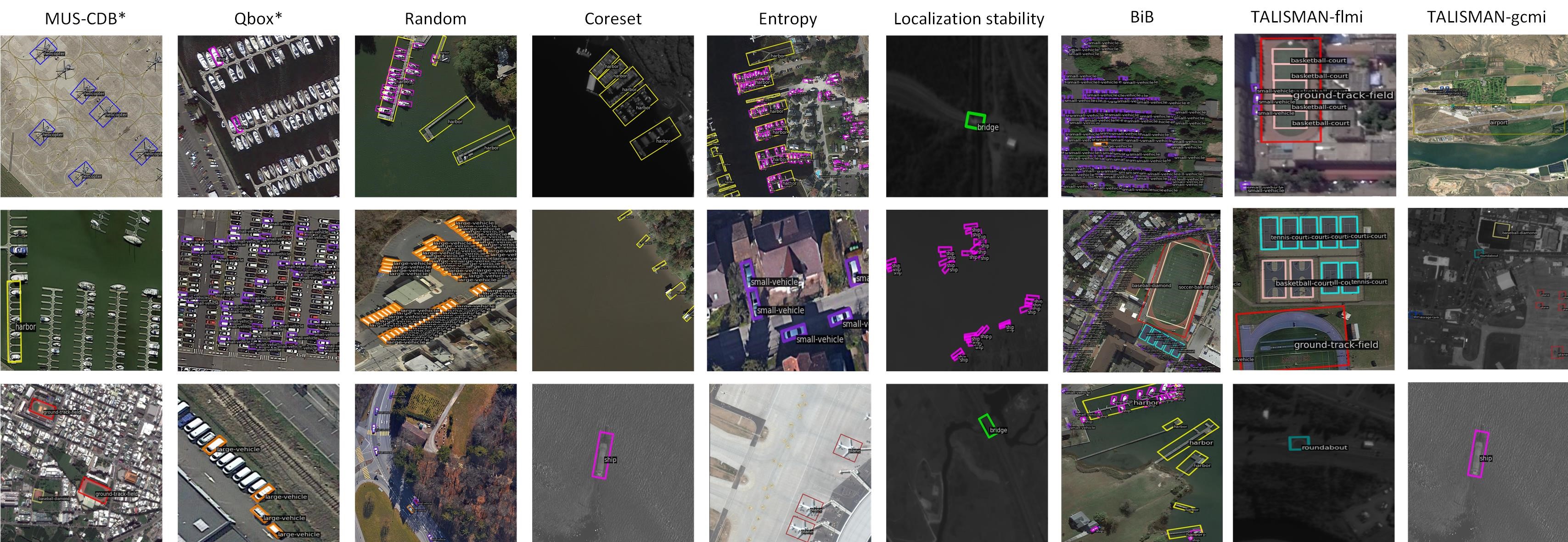
Figure 5: Examples of the top-rated objects or images queried by MUS-CDB, Qbox [5], Random, Coreset [40], Entropy [29], Localization Stability [4], BiB [53], TALISMAN-flmi [54] and TALISMAN-gcmi [54] on the DOTA-v2.0 [14]. * denotes that the AL method follows the object-based query type. The visual comparison results in the first and second columns show that our proposed method MUS-CDB can sample more valuable middle and rare classes than another object-based sampling method Qbox. In addition, compared with other image-based sampling methods, it can be found that MUS-CDB can effectively save sampling costs through object-based sampling and then sampling more diverse objects.

TABLE IV: Comparison of mAP(%) for ReDet [21] on DOTA-v2.0  [14] validation set with different score thresholds in Equ. 5 of Mixed Uncertainty Sampling module (MUS). The Cycle-0 column reports the performance without any active learning sampling strategy.

$\theta$	Cycle-0	Cycle-1	Cycle-2	Cycle-3	Cycle-4
0.05	22.8	30.8	36.7	39.4	40.6
0.10	22.8	34.1	37.2	40.2	40.9
0.15	22.8	32.7	37.1	39.4	40.4

IV-B3 Score Threshold $\theta$

$\theta$ is the parameter of module MUS in Equ. (5), which is used to impose preference on the images with distinct information in the active selection phase. According to the results in Table IV, the optimal value of $\theta$ is obtained around 0.10. Therefore, we use $\theta$ = 0.10 for all our experiments. This can be explained by the fact that when $\theta$ is close to the lower bound of 0.05, more noise is involved in calculating the image uncertainty score. Therefore the final object information calculation is inaccurate. Conversely, if $\theta$ becomes larger, the performance degrades. This is because predicted bounding boxes containing rare patterns in the image are filtered because of low predicted scores and cannot participate in calculating image information.

IV-B4 Visualization of the Queried Boxes

To demonstrate whether MUS-CDB selects the expected objects for sampling, we visualize the top-ranked objects sampled by the object-based sampling method MUS-CDB versus Qbox and the top-ranked images sampled by the image-based sampling methods random, entropy, Coreset, and localization stability. According to Figure 5, we can see that our method MUS-CDB can preferentially sample informative examples of rare categories, such as [helicopter], [baseball diamond], [ground track field], and [soccer-ball field]. The sampling results of the random method are consistent with the original category distribution of the DOTA-v2.0 dataset, manifested in over-sampling the low-informative head categories and intermediate categories such as [plane], [ship], [small vehicle], and [large vehicle]. As an object-based sampling method, Qbox oversamples common categories, such as the classes [small vehicle], [large vehicle], and [ship], and fails to sample rare categories. Entropy (the image-based sampling method) results in most of the queried samples being in the same pattern, leading to information redundancy. The images sampled by the Coreset and Localization Stability methods have a single land type. The Coreset method preferentially samples images in the ocean background, and the Localization Stability method preferentially samples images in the dark scenes. The sample distribution in the images collected by the two methods is relatively sparse, which can effectively alleviate the problem of redundant annotation. However, the two methods pay too little attention to the rare category, resulting in a low-performance improvement of the final model. The BiB method is prone to over-sampling densely distributed images, which is not a significant issue in generic scenarios where objects are sparsely distributed in images. However, in remote sensing scenarios, this can lead to redundant sampling due to the dense distribution of the same object categories in the images, which can limit the effectiveness of the sampling method in improving the overall performance of the final model. The TALISMAN method introduces rare categories as reference objects to help the sampling method collect more samples of rare categories. However, compared to our proposed method, it lacks an overall improvement in performance for all categories.

TABLE V: Ablation studies on strategies of Mixed Uncertainty Sampling module (MUS), Class Distribution Balancing module (CDB) based on mAP(%). The Cycle-0 column reports the performance without any active learning sampling strategy.

Method	MUS	CDB	Cycle-0	Cycle-1	Cycle-2	Cycle-3	Cycle-4
Random			22.8	24.6	25.1	25.3	26.2
(a)	✓		22.8	33.0	36.2	38.1	39.9
(b)		✓	22.8	32.9	37.0	37.3	40.5
(d)	✓	✓	22.8	34.1	37.2	40.2	40.9

IV-C Ablation Study

IV-C1 Evaluation on each component of MUS-CDB

To further investigate the effectiveness of each component of MUS-CDB, we conduct ablation experiments on the DOTA-v2.0 task. As shown in Table V, satisfactory and consistent gains from the Random baseline to our whole method demonstrate the validity of each module. From Table V we can see that both MUS and CDB module has achieved significant performance improvements compared to the Random baseline. The results in Table V demonstrate that both the MUS and CDB modules contribute significantly to the overall performance of MUS-CDB, and together they provide a more effective and efficient way of selecting highly informative predicted bounding boxes for training object detection models.

TABLE VI: Comparison of mAP(%) for ReDet [21] on DOTA-v2.0 [14] validation set for evaluating the effectiveness of MUS Method via ablation experiment: Entropy-Based Uncertainty Sampling (Method 1) vs. MUS Method (Method 2). The Cycle-0 column reports the performance without any active learning sampling strategy.

Method	Cycle-0	Cycle-1	Cycle-2	Cycle-3	Cycle-4
(1)	22.8	30.8	35.2	36.2	38.4
(2)	22.8	33.0	36.2	38.1	39.9

IV-C2 Evaluation on the image-level term of MUS

To further investigate the effectiveness of the proposed method, we conducted ablation experiments specifically targeting the image-level term proposed in the MUS. We conducted these experiments on the DOTA-v2.0 dataset, and the results are summarized in Table VI. As we can see from the table, incorporating global information into the calculation of sample informativeness (i.e., adding the image-level term to the original entropy-based uncertainty measurement) leads to a significant improvement in detection performance compared to using the original entropy-based uncertainty measurement alone. This improvement demonstrates that incorporating spatial and semantic information from the image can benefit object detection tasks in remote sensing scenarios. The proposed MUS module is a valuable addition to the MUS-CDB framework. In summary, our ablation experiments provide strong evidence supporting the effectiveness of the proposed image-level term in the MUS module and demonstrate the importance of considering both the image-level and instance-level information in the MUS-CDB framework for achieving better object detection performance in remote sensing applications.

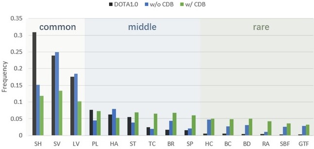
Figure 6: The average category frequency (%) of DOTA-v1.0 [13] sampled by our AL methods in each round with ReDet [21]. Our proposed Class Distribution Balancing module (CDB) can sample more middle and rare and fewer common categories.

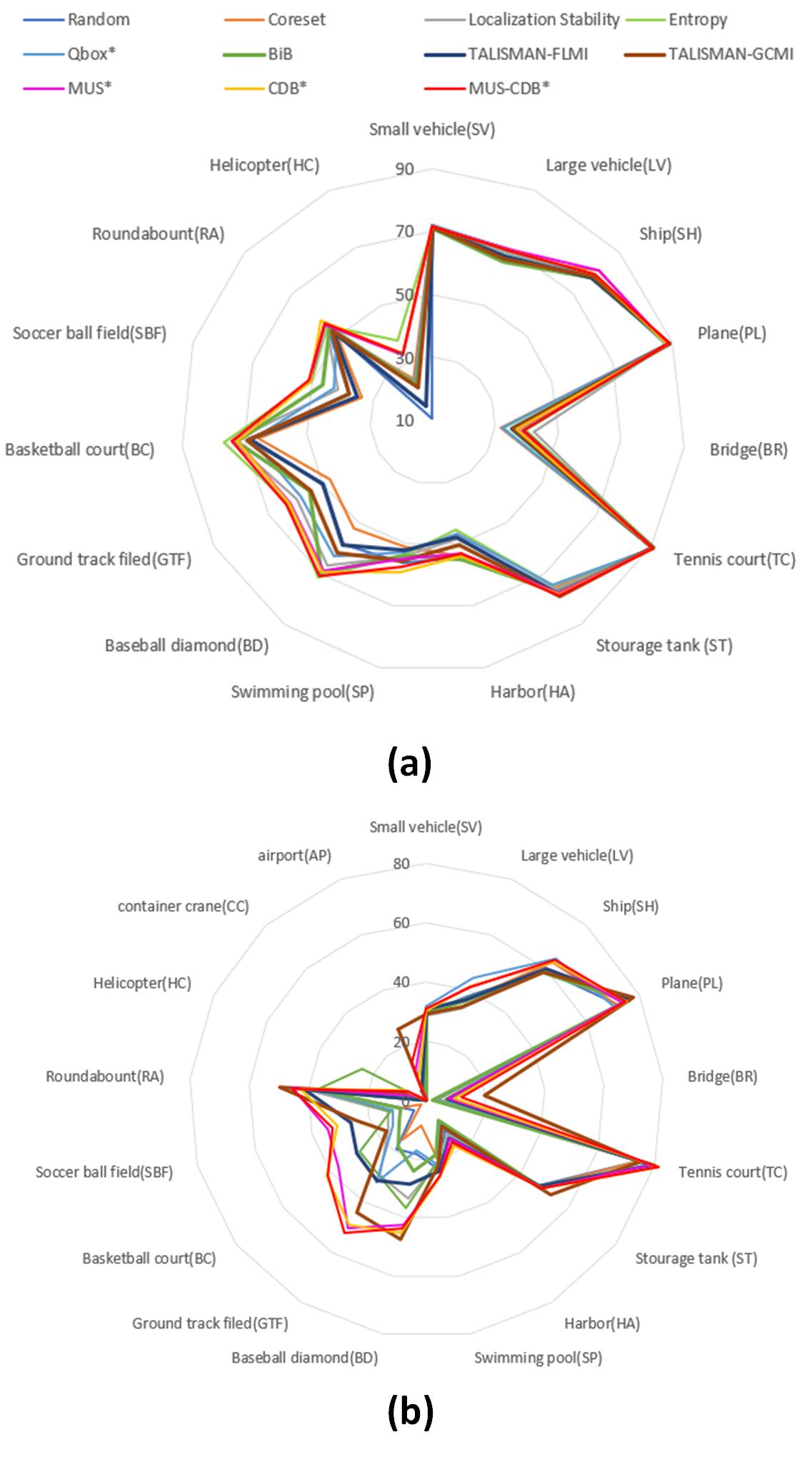
Figure 7: Radar charts for each category of objects in different datasets. (a) DOTA-v1.0 [13]. (b) DOTA-v2.0 [14]. Different colors represent different active learning methods. The larger area enclosed by the outer line, the better performance of the corresponding method. The value in this graph denotes the average AP over five cycles of active learning.

IV-C3 Analysis of Queried Class Distribution using CDB Method

Figure 6 shows the class frequency of the DOTA-v1.0 dataset and the average class frequency of training samples selected by our methods in each cycle of AL. The actual distribution of each class in the DOTA-v1.0 is exactly long-tailed. Most AL methods tend to select many common categories for annotation, resulting in ineffective and redundant sampling. The CDB module in our method enables us to allocate this problem in middle and rare categories such as [tennis court], [bridge], [swimming pool], [basketball court], [baseball diamond], and [roundabout] as shown in the green column of Figure 6. This approach produces more diverse and balanced samples for annotation and avoids being influenced by the dataset’s distribution. This improvement demonstrates the unique contribution of the CDB module to our method, which other active learning methods may not have considered. Our method provides a more effective and efficient approach for addressing the long-tail distribution problem in object detection datasets. The performance superiority of our method over other methods in each category is visualized in Figure 7.

TABLE VII: Comparison of mAP(%) for ReDet [21] on DOTA-v2.0 [14] validation set for the MUS-CDB Method using ReDet’s Loss Function and Improved Loss Function: Method 1 with Default Loss Function vs. Method 2 with Proposed Improved Loss Function. The Cycle-0 column reports the performance without any active learning sampling strategy.

Method	Cycle-0	Cycle-1	Cycle-2	Cycle-3	Cycle-4
(1)	22.8	32.4	36.3	38.3	39.9
(2)	22.8	34.1	37.2	40.2	40.9

IV-C4 Evaluation on proposed loss function

To further evaluate the proposed loss function’s effectiveness in the MUS-CDB context, we conducted experiments on DOTA-v2.0 to compare the performance of MUS-CDB using the original loss function and the proposed modified loss function. The experimental results are presented in Table VII. As we can see from the table, using the proposed modified loss function leads to a significant improvement in detection performance compared to using the original loss function. This improvement demonstrates the effectiveness of the proposed loss function in reducing the noise introduced by partially annotated images during model training and improving the robustness of the model to such noisy inputs. One possible reason why the proposed loss function is effective is that it adaptively adjusts the classification loss weight for background samples. This helps the model assign less weight to the background samples likely to be noisy or ambiguous and more weight to the informative samples that can contribute to the model training more effectively. This can help reduce the impact of noisy and ambiguous samples on the model training and improve the overall performance of the model.

V Conclusion

In this paper, we propose an object-based active learning method MUS-CDB to alleviate the massive burden of aerial object detection data annotation. We devise an image- and object-guided uncertainty sampling selection criterion in active querying to identify the most informative instances. We consider the long-tailed problem of the remote sensing image dataset and impose class preference during active sampling to promote the diversity of selected objects. An effective training method for partially labeled data is also proposed to utilize the queried knowledge. Extensive experiments on the DOTA-v1.0 and DOTA-v2.0 benchmarks demonstrate the superiority of the proposed MUS-CDB.

Dong Liang received a B.S. degree in Telecommunication Engineering and an M.S. in Circuits and Systems from Lanzhou University, China, in 2008 and 2011, respectively. In 2015, he received Ph.D. at the Graduate School of IST, Hokkaido University, Japan. He is an associate professor at the College of Computer Science and Technology, Nanjing University of Aeronautics and Astronautics. His research interests include pattern recognition and image processing. He was awarded the Excellence Research Award from Hokkaido University in 2013. He has published several research papers including in IEEE TIP/TNNLS/TMM/TGRS/TCSVT, Pattern Recognition, AAAI, and IJCAI.

Jing-Wei Zhang received the B.S. degree in computer science and technology from Jiangsu University, Zhenjiang, China, in 2021. She is pursuing a master’s degree with the College of Computer Science and Technology, Nanjing University of Aeronautics and Astronautics, Nanjing. Her research interests include active learning and object detection.

Ying-Peng Tang received the BSc degree from the Nanjing University of Aeronautics and Astronautics, China, in 2020. He is currently pursuing a Ph.D. degree in computer science and technology with the Nanjing University of Aeronautics and Astronautics, Nanjing, China. His current research interests include active learning and semi-supervised learning. He was awarded for China National Scholarship in 2022 and the Excellent Master thesis in Jiangsu Province in 2021.

Sheng-Jun Huang received the BSc and Ph.D. degrees in computer science from Nanjing University, China, in 2008 and 2014, respectively. He is now a professor at the College of Computer Science and Technology at Nanjing University of Aeronautics and Astronautics. His main research interests include machine learning and data mining. He has been selected for the Young Elite Scientists Sponsorship Program by CAST in 2016, and won the China Computer Federation Outstanding Doctoral Dissertation Award in 2015, the KDD Best Poster Award in 2012, and the Microsoft Fellowship Award in 2011. He is a Junior Associate Editor of Frontiers of Computer Science.

References

- [1] X. X. Zhu, D. Tuia, L. Mou, G.-S. Xia, L. Zhang, F. Xu, and F. Fraundorfer, “Deep learning in remote sensing: A comprehensive review and list of resources,” IEEE Geoscience and Remote Sensing Magazine, vol. 5, no. 4, pp. 8–36, 2017.
- [2] Y. Hua, L. Mou, and X. X. Zhu, “Relation network for multilabel aerial image classification,” IEEE Transactions on Geoscience and Remote Sensing, vol. 58, no. 7, pp. 4558–4572, 2020.
- [3] L. Zhang and L. Zhang, “Artificial intelligence for remote sensing data analysis: A review of challenges and opportunities,” IEEE Geoscience and Remote Sensing Magazine, vol. Early Access, pp. 1–16, 2022.
- [4] C.-C. Kao, T.-Y. Lee, P. Sen, and M.-Y. Liu, “Localization-aware active learning for object detection,” in Asian Conference on Computer Vision, pp. 506–522, Springer, 2018.
- [5] Y.-P. Tang, X.-S. Wei, B. Zhao, and S.-J. Huang, “Qbox: Partial transfer learning with active querying for object detection,” IEEE Transactions on Neural Networks and Learning Systems, 2021.
- [6] S. V. Desai and V. N. Balasubramanian, “Towards fine-grained sampling for active learning in object detection,” in Proceedings of the IEEE/CVF Conference on Computer Vision and Pattern Recognition Workshops, pp. 924–925, 2020.
- [7] S. Roy, A. Unmesh, and V. P. Namboodiri, “Deep active learning for object detection.,” in BMVC, p. 91, 2018.
- [8] Q. Wang, Y. Liu, Z. Xiong, and Y. Yuan, “Hybrid feature aligned network for salient object detection in optical remote sensing imagery,” IEEE Transactions on Geoscience and Remote Sensing, vol. 60, pp. 1–15, 2022.
- [9] F. Li, S. Li, C. Zhu, X. Lan, and H. Chang, “Cost-effective class-imbalance aware cnn for vehicle localization and categorization in high resolution aerial images,” Remote Sensing, vol. 9, no. 5, p. 494, 2017.
- [10] K.-P. Ning, X. Zhao, Y. Li, and S.-J. Huang, “Active learning for open-set annotation,” in Proceedings of the IEEE/CVF Conference on Computer Vision and Pattern Recognition, pp. 41–49, 2022.
- [11] N. Xu, C. Huo, J. Guo, Y. Liu, J. Wang, and C. Pan, “Adaptive remote sensing image attribute learning for active object detection,” in 2020 25th International Conference on Pattern Recognition (ICPR), pp. 111–118, IEEE, 2021.
- [12] G. Xu, X. Zhu, and N. Tapper, “Using convolutional neural networks incorporating hierarchical active learning for target-searching in large-scale remote sensing images,” International Journal of Remote Sensing, vol. 41, no. 11, pp. 4057–4079, 2020.
- [13] G.-S. Xia, X. Bai, J. Ding, Z. Zhu, S. Belongie, J. Luo, M. Datcu, M. Pelillo, and L. Zhang, “Dota: A large-scale dataset for object detection in aerial images,” in Proceedings of the IEEE conference on computer vision and pattern recognition, pp. 3974–3983, 2018.
- [14] J. Ding, N. Xue, G.-S. Xia, X. Bai, W. Yang, M. Y. Yang, S. Belongie, J. Luo, M. Datcu, M. Pelillo, et al., “Object detection in aerial images: A large-scale benchmark and challenges,” IEEE transactions on pattern analysis and machine intelligence, vol. 44, no. 11, pp. 7778–7796, 2021.
- [15] J. Ma, W. Shao, H. Ye, L. Wang, H. Wang, Y. Zheng, and X. Xue, “Arbitrary-oriented scene text detection via rotation proposals,” IEEE Transactions on Multimedia, vol. 20, no. 11, pp. 3111–3122, 2018.
- [16] Z. Zhang, W. Guo, S. Zhu, and W. Yu, “Toward arbitrary-oriented ship detection with rotated region proposal and discrimination networks,” IEEE Geoscience and Remote Sensing Letters, vol. 15, no. 11, pp. 1745–1749, 2018.
- [17] J. Ding, N. Xue, Y. Long, G.-S. Xia, and Q. Lu, “Learning roi transformer for oriented object detection in aerial images,” in Proceedings of the IEEE/CVF Conference on Computer Vision and Pattern Recognition, pp. 2849–2858, 2019.
- [18] X. Pan, Y. Ren, K. Sheng, W. Dong, H. Yuan, X. Guo, C. Ma, and C. Xu, “Dynamic refinement network for oriented and densely packed object detection,” in Proceedings of the IEEE/CVF Conference on Computer Vision and Pattern Recognition, pp. 11207–11216, 2020.
- [19] Z. Wei, D. Liang, D. Zhang, L. Zhang, Q. Geng, M. Wei, and H. Zhou, “Learning calibrated-guidance for object detection in aerial images,” IEEE Journal of Selected Topics in Applied Earth Observations and Remote Sensing, vol. 15, pp. 2721–2733, 2022.
- [20] X. Yang and J. Yan, “Arbitrary-oriented object detection with circular smooth label,” in European Conference on Computer Vision, pp. 677–694, Springer, 2020.
- [21] J. Han, J. Ding, N. Xue, and G.-S. Xia, “Redet: A rotation-equivariant detector for aerial object detection,” in Proceedings of the IEEE/CVF Conference on Computer Vision and Pattern Recognition, pp. 2786–2795, 2021.
- [22] Z. Sun, X. Leng, Y. Lei, B. Xiong, K. Ji, and G. Kuang, “Bifa-yolo: A novel yolo-based method for arbitrary-oriented ship detection in high-resolution sar images,” Remote Sensing, vol. 13, no. 21, p. 4209, 2021.
- [23] H. Qiu, H. Li, Q. Wu, F. Meng, K. N. Ngan, and H. Shi, “A2rmnet: Adaptively aspect ratio multi-scale network for object detection in remote sensing images,” Remote Sensing, vol. 11, no. 13, p. 1594, 2019.
- [24] Z. Li, H. Shen, Q. Cheng, Y. Liu, S. You, and Z. He, “Deep learning based cloud detection for medium and high resolution remote sensing images of different sensors,” ISPRS Journal of Photogrammetry and Remote Sensing, vol. 150, pp. 197–212, 2019.
- [25] Z. Zheng, Y. Zhong, A. Ma, X. Han, J. Zhao, Y. Liu, and L. Zhang, “Hynet: Hyper-scale object detection network framework for multiple spatial resolution remote sensing imagery,” ISPRS Journal of Photogrammetry and Remote Sensing, vol. 166, pp. 1–14, 2020.
- [26] D. Liang, Q. Geng, Z. Wei, D. A. Vorontsov, E. L. Kim, M. Wei, and H. Zhou, “Anchor retouching via model interaction for robust object detection in aerial images,” IEEE Transactions on Geoscience and Remote Sensing, vol. 60, pp. 1–13, 2021.
- [27] Y. Liu, Q. Li, Y. Yuan, Q. Du, and Q. Wang, “Abnet: Adaptive balanced network for multiscale object detection in remote sensing imagery,” IEEE Transactions on Geoscience and Remote Sensing, vol. 60, pp. 1–14, 2021.
- [28] Y. Liu, Q. Li, Y. Yuan, and Q. Wang, “Single-shot balanced detector for geospatial object detection,” in ICASSP 2022-2022 IEEE International Conference on Acoustics, Speech and Signal Processing (ICASSP), pp. 2529–2533, IEEE, 2022.
- [29] B. Settles, “Active learning literature survey,” 2009.
- [30] S. Sinha, S. Ebrahimi, and T. Darrell, “Variational adversarial active learning,” in Proceedings of the IEEE/CVF International Conference on Computer Vision, pp. 5972–5981, 2019.
- [31] S. Ebrahimi, W. Gan, D. Chen, G. Biamby, K. Salahi, M. Laielli, S. Zhu, and T. Darrell, “Minimax active learning,” arXiv preprint arXiv:2012.10467, 2020.
- [32] W. H. Beluch, T. Genewein, A. Nürnberger, and J. M. Köhler, “The power of ensembles for active learning in image classification,” in Proceedings of the IEEE conference on computer vision and pattern recognition, pp. 9368–9377, 2018.
- [33] H. H. Aghdam, A. Gonzalez-Garcia, J. v. d. Weijer, and A. M. López, “Active learning for deep detection neural networks,” in Proceedings of the IEEE/CVF International Conference on Computer Vision, pp. 3672–3680, 2019.
- [34] D. Yoo and I. S. Kweon, “Learning loss for active learning,” in Proceedings of the IEEE/CVF conference on computer vision and pattern recognition, pp. 93–102, 2019.
- [35] L. Cai, X. Xu, J. H. Liew, and C. S. Foo, “Revisiting superpixels for active learning in semantic segmentation with realistic annotation costs,” in Proceedings of the IEEE/CVF Conference on Computer Vision and Pattern Recognition, pp. 10988–10997, 2021.
- [36] A. Casanova, P. O. Pinheiro, N. Rostamzadeh, and C. J. Pal, “Reinforced active learning for image segmentation,” arXiv preprint arXiv:2002.06583, 2020.
- [37] T. Kasarla, G. Nagendar, G. M. Hegde, V. Balasubramanian, and C. Jawahar, “Region-based active learning for efficient labeling in semantic segmentation,” in 2019 IEEE Winter Conference on Applications of Computer Vision (WACV), pp. 1109–1117, IEEE, 2019.
- [38] Y. Yan and S.-J. Huang, “Cost-effective active learning for hierarchical multi-label classification.,” in IJCAI, pp. 2962–2968, 2018.
- [39] A. Kirsch, J. Van Amersfoort, and Y. Gal, “Batchbald: Efficient and diverse batch acquisition for deep bayesian active learning,” pp. 7024–7035, 2019.
- [40] O. Sener and S. Savarese, “Active learning for convolutional neural networks: A core-set approach,” arXiv preprint arXiv:1708.00489, 2017.
- [41] S.-J. Huang, R. Jin, and Z.-H. Zhou, “Active learning by querying informative and representative examples,” Advances in neural information processing systems, pp. 1936–1949, 2010.
- [42] Y.-P. Tang and S.-J. Huang, “Self-paced active learning: Query the right thing at the right time,” in Proceedings of the AAAI conference on artificial intelligence, pp. 5117–5124, 2019.
- [43] J. T. Ash, C. Zhang, A. Krishnamurthy, J. Langford, and A. Agarwal, “Deep batch active learning by diverse, uncertain gradient lower bounds,” arXiv preprint arXiv:1906.03671, 2019.
- [44] S. Agarwal, H. Arora, S. Anand, and C. Arora, “Contextual diversity for active learning,” in European Conference on Computer Vision, pp. 137–153, Springer, 2020.
- [45] K. Wang, X. Yan, D. Zhang, L. Zhang, and L. Lin, “Towards human-machine cooperation: Self-supervised sample mining for object detection,” in Proceedings of the IEEE Conference on Computer Vision and Pattern Recognition, pp. 1605–1613, 2018.
- [46] M. Laielli, G. Biamby, D. Chen, A. Loeffler, P. D. Nguyen, R. Luo, T. Darrell, and S. Ebrahimi, “Region-level active learning for cluttered scenes,” arXiv preprint arXiv:2108.09186, 2021.
- [47] B. Xie, L. Yuan, S. Li, C. H. Liu, and X. Cheng, “Towards fewer annotations: Active learning via region impurity and prediction uncertainty for domain adaptive semantic segmentation,” in Proceedings of the IEEE/CVF Conference on Computer Vision and Pattern Recognition, pp. 8068–8078, 2022.
- [48] Z. Liang, X. Xu, S. Deng, L. Cai, T. Jiang, and K. Jia, “Exploring diversity-based active learning for 3d object detection in autonomous driving,” arXiv preprint arXiv:2205.07708, 2022.
- [49] X. Xie, G. Cheng, J. Wang, X. Yao, and J. Han, “Oriented r-cnn for object detection,” in Proceedings of the IEEE/CVF International Conference on Computer Vision, pp. 3520–3529, 2021.
- [50] X. Yang, X. Yang, J. Yang, Q. Ming, W. Wang, Q. Tian, and J. Yan, “Learning high-precision bounding box for rotated object detection via kullback-leibler divergence,” Advances in Neural Information Processing Systems, pp. 18381–18394, 2021.
- [51] L. Hou, K. Lu, J. Xue, and Y. Li, “Shape-adaptive selection and measurement for oriented object detection,” in Proceedings of the AAAI Conference on Artificial Intelligence, pp. 923–932, 2022.
- [52] S. Ren, K. He, R. Girshick, and J. Sun, “Faster r-cnn: Towards real-time object detection with region proposal networks,” Advances in neural information processing systems, vol. 28, pp. 91–99, 2015.
- [53] H. V. Vo, O. Siméoni, S. Gidaris, A. Bursuc, P. Pérez, and J. Ponce, “Active learning strategies for weakly-supervised object detection,” in Computer Vision–ECCV 2022: 17th European Conference, Tel Aviv, Israel, October 23–27, 2022, Proceedings, Part XXX, pp. 211–230, Springer, 2022.
- [54] S. Kothawade, S. Ghosh, S. Shekhar, Y. Xiang, and R. Iyer, “Talisman: targeted active learning for object detection with rare classes and slices using submodular mutual information,” in Computer Vision–ECCV 2022: 17th European Conference, Tel Aviv, Israel, October 23–27, 2022, Proceedings, Part XXXVIII, pp. 1–16, Springer, 2022.
- [55] A. Krizhevsky, I. Sutskever, and G. E. Hinton, “Imagenet classification with deep convolutional neural networks,” Communications of the ACM, vol. 60, no. 6, pp. 84–90, 2017.