Solvable Limits of a class of generalized Vector Nonlocal Nonlinear Schrödinger equation with balanced loss-gain

Abstract

We consider a class of one dimensional Vector Nonlocal Non-linear Schrödinger Equation (VNNLSE) in an external complex potential with time-modulated Balanced Loss-Gain(BLG) and Linear Coupling(LC) among the components of Schrödinger fields, and space-time dependent nonlinear strength. The system admits Lagrangian and Hamiltonian formulations under certain conditions. It is shown that various dynamical variables like total power, $\cal{PT}$-symmetric Hamiltonian, width of the wave-packet and its speed of growth, etc. are real-valued despite the Hamiltonian density being complex-valued. We study the exact solvability of the generic VNNLSE with or without a Hamiltonian formulation. In the first part, we study time-evolution of moments which are analogous to space-integrals of Stokes variables and find condition for existence of solutions which are bounded in time. In the second part, we use a non-unitary transformation followed by a coordinate transformation to map the VNNLSE to various solvable equations. The coordinate transformation is not required at all for the limiting case when non-unitary transformation reduces to pseudo-unitary transformation. The exact solutions are bounded in time for the same condition which is obtained through the study of time-evolution of moments. Various exact solutions of the VNNLSE are presented.

1 Introduction

Nonlinear Schrödinger equation(NLSE) appears in many fields of science like optics in nonlinear media[1, 2, 3], Bose-Einstein condensates (BEC)[4, 5, 6, 7], gravity waves[8], plasma physics[9], Bio-molecular dynamics[10] etc. Several generalisations of NLSE have been considered over the past few decades. One aspect of generalisations of NLSE is to introduce non-local nonlinear interaction. Nonlocal nonlinearity arises whenever the nonlinear effect at a particular point depends on the influences from other points and it arises in many cases like Bose-Einstein condensation in a system having long range interaction[11, 12], transport process associated with heat conduction in media having a thermal influence, and during diffusion of charge carriers, atoms, or molecules in atomic vapours[13, 14]. In case of optical beams in nonlinear dielectric wave-guides or wave-guide arrays with random variation of refractive index size or wave-guide spacing, the effect of nonlocal nonlinearity becomes relevant[15]. Nonlocal nonlinearities also arise in long-range interactions of molecules in nematic liquid crystals[16].

The exact solvability and integrability of non-local NLSE(NNLSE) have been studied in the last few years. Integrable NNLSE was introduced by Ablowitz and Musslimani[17] and it admits both the bright and dark solitons for the same range of nonlinear strength[18]. The nonlocal vector NLSE is also integrable and soliton solution of the same equation is obtained through inverse scattering methods[19]. A discrete version of NNLSE has been shown to be exactly solvable and one soliton solution has been constructed [20]. Further, exact solutions of a class of NNLSE with confining potential like Harmonic trap, reflection-less potential and other $\cal{PT}$ symmetric complex potentials, have been obtained [21]. Various generalisations of the NNLSE having mathematical and physical importance have been considered[18, 22, 23, 24, 25, 26, 27, 28, 29, 30, 31, 32, 33, 34, 35, 36]. The dynamical behaviour of continuous and discrete NNLSE having $\cal{PT}$ invariant nonlinearity has been studied in Ref. [18]. It is shown in Ref. [22] that NNLSE is gauge equivalent to physically important magnetic structure. For a number of nonlocal nonlinear equations, periodic and hyperbolic soliton solutions are reported in Ref. [25]. Applying the N-th iterated Darboux transformation, a chain of non-singular localised wave solution which can describe the soliton interactions on continuous wave background, is derived for a NNLSE [26]. Localized nonlinear modes of self-focusing and defocusing NNLSE equation with $\cal{PT}$-symmetric complex potential like Rosen-Morse, Periodic, Scarf-II potential, are reported in Ref. [30].

Over the past few years, systems with balanced loss and gain(BLG) have received considerable attention in the literature[37, 38, 39]. Within this context, NLSE with BLG is known to admit bright[40, 41] and dark solitons[42], breathers[43, 44], rogue waves[45], exceptional points[46, 44] etc. Soliton solution was found in the discrete non-linear Schr$\ddot{o}$dinger equation with gain and loss[47]. Stabilisation of soliton by the periodic time-dependent BLG and LC parameters has been studied[44]. A specific model[48] with constant BLG and LC terms show power oscillations that may have interesting technological applications. Most of the papers dealing with the BLG system use approximation and numerical methods. A possible technique for obtaining exact solutions of coupled NLSE with arbitrary time dependent BLG parameters has been given in Ref.[49]. It has been shown in Ref.[50] that local and nonlocal vector NLSE with BLG is integrable when the matrix representing the linear term is pseudo-hermitian with respect to the hermitian matrix comprising the generic cubic nonlinearity.

The article aims at identifying exactly solvable cases of VNNLSE in an external complex potential with BLG and LC among the components of Schr$\ddot{o}$dinger fields. The BLG and LC terms are allowed to be time dependent while the strength of nonlinear interactions is space-time dependent. The VNNLSE is a nonlocal generalization of the system discussed in Ref. [49] and may be used to model different physical phenomena wherein nonlocal interaction is present. We show that the system admits Hamiltonian and Lagrangian formulations under certain conditions. The subtleties involved in deriving Euler-Lagrange equations of motion and conserved Noether charges associated with continuous internal symmetry for non-hermitian Lagrangian are discussed. Further, we show that various dynamical variables like charge, $\cal{PT}$-symmetric Hamiltonian, width of the wave packets and its speed of growth, etc. are real valued despite the Hamiltonian density being complex valued.

We investigate the exact solvability of the generic VNNLSE with or without a Hamiltonian formulation. The study involves various combinations of time-dependent BLG, LC, external complex potential and space-time modulated nonlinear interaction. The time-evolution of certain moments, analogous to space-integrals of the familiar Stokes variables, is determined in terms of a set of coupled first order ordinary differential equations which is solved analytically. The method is an indirect way of studying collapse or growth of the wave-packet and has been used earlier[51]. The exact solution of the system under investigation also allows to identify the regions in the parameter-space which admit bounded or unbounded solution in time. It should be noted that exact space-like dependence of the Schrödinger field can not be unearthed in this method. Nevertheless, it is an useful tool to study the bounded nature of the solution.

In the next step, we investigate the limits in which exact, analytical solution of the fields may be obtained. The BLG and LC terms may be removed completely from the VNNLSE through non-unitary transformations provided the time-modulations of the BLG and LC terms are identical[49]. In general, the non-unitary transformation modifies the nonlinear term by imparting additional time-dependence. However, for the special case in which the nonlinear interaction may be identified as the non-local analogue of the Manakov-Zakharov-Schulman(MZS) system, even the nonlinear interaction remains unchanged. The non-unitary transformation reduces to the pseudo-unitary[52] transformation under this situation. It should be noted that this is not a symmetry transformation, since it does not keep the system invariant. Further, unlike the unitary transformations, the non-unitary and pseudo-unitary transformations do not preserve the norm. Thus, the removal of of the BLG and LC terms can not be thought of as gauge transformations. The mapping is used to construct many exact solutions of the system for generic time-modulations of the BLG and LC terms and a large class of complex external potentials.

We also investigate the system for which the non-unitary transformation removes the BLG and LC terms at the cost of modifying the nonlinear term. A co-ordinate transformation, as already discussed in ref. [7, 49, 53], is used to map the modified VNNLSE to solvable equation. One essential condition for this co-ordinate transformation is that the transformed spatial co-ordinate is odd under parity transformation of original one. This condition is not applicable for its local counterpart [49]. We present many exact solutions.

The plan of the article is as follows. The model is introduced in Sec-2. The Lagrangian and Hamiltonian of the system are constructed in Sec.-2.1. The real valuedness of different dynamical variables like charge, Hamiltonian, width of wave packets etc. are shown. The study of the systems in terms of moments which are defined in terms of space-integrals of Stokes variables, are presented in the sec-2.2. In Sec-3, the VNNLSE is mapped to various solvable equations. We present the solution for the case of a $M$-pseudo-hermitian $A$ in Sec. 3.1. A few exact solutions for $V(x)=0$ are presented in Sec-3.1.1. The exact solutions for a few non-vanishing complex confining potentials are presented in Sec-3.1.2. The general method for which $A$ is not $M$-pseudo-hermitian is presented in Sec-3.2. Finally the findings are summarized in Sec-4. In Appendix-I, several exact solutions for the case of pseudo-hermitian loss-gain matrix have been presented.

2 The Model

We consider a VNNLSE with time-dependent BLG in terms of a complex scalar field $\Psi(x,t)=(\psi_{1}\ \ \psi_{2})^{T}$ with two components $\psi_{1}(x,t)$ and $\psi_{2}(x,t)$, where the superscript ^T denotes the transpose of a matrix. The VNNLSE with BLG has the form:

$$i\psi_{1t} = -\psi_{1xx}+k^{*}(t)\psi_{2}+i\gamma(t)\psi_{1}+V(x,t)\psi_{1}$$

$$+ \sum_{i,j=1}^{2}\left[l_{ij}(x,t)\ \psi_{i}^{*}(-x,t)\psi_{j}(x,t)\right]\psi_{1}$$

$$i\psi_{2t} = -\psi_{2xx}+k(t)\psi_{1}-i\gamma(t)\psi_{2}+V(x,t)\psi_{2}$$ (1)

$$+ \sum_{i,j=1}^{2}\left[m_{ij}(x,t)\ \psi_{i}^{*}(-x,t)\psi_{j}(x,t)\right]\ \psi_{2}$$

where $\psi_{it}$ and $\psi_{ixx}$ denote partial derivative of $\psi_{i}$ with respect to $t$ and second order partial derivative of $\psi_{i}$ with respect to $x$, respectively. The time-dependent parameters $k(t)$ and $\gamma(t)$ denote the strengths of the LC and the BLG, respectively. The space-time dependent real parameters $l_{ij}(x,t)$ and $m_{ij}(x,t)$ denote the strengths of the cubic nonlinearity. In the context of optics, with $l_{11}$ and $m_{22}$ can be identified as self-phase modulations, whereas $l_{12}$, $m_{11}$ can be identified as cross-phase modulation. The external confining potential $V(x,t)$ appears in the context of Bose-Einstein Condensates[6], which is taken to be complex i.e. $V(x,t)=S(x,t)+i\tilde{S}(x,t)$ . There are many solvable limits of Eq.(1), with the simplest case $l_{ij}=m_{ij}=0,\forall i,j$, which models the optical wave propagation under paraxial approximation[54, 55]. With $M=L$ and vanishing LC, BLG and external potential, the system reduces to the nonlocal analogue of MZS system[56, 57, 58]. A ${\cal PT}$-symmetry preserving breathing one-soliton solution has been constructed for the nonlocal Manakov equation through inverse scattering transform[19].

We define an operator $D_{0}=\sigma_{0}\frac{\partial}{\partial t}+iA(t)$, where the $2\times 2$ matrix $A(t)$ is expressed as $A(t)=k\sigma_{-}+k^{*}\sigma_{+}+i\gamma\sigma_{3}$ and $\sigma_{\pm}=\frac{1}{2}(\sigma_{1}\pm i\sigma_{2})$. $\sigma_{0}$ is a $2\times 2$ identity matrix and $\sigma_{j}$’s, $j=1,2,3$ are pauli matrices. We also define the projection operator $P_{\pm}$ as $P_{\pm}=\frac{1}{2}(\sigma_{0}\pm\sigma_{3})$ with the property $P_{+}\Psi=(\psi_{1}\ 0)^{T}$ and $P_{-}\Psi=(0\ \psi_{2})^{T}$. Eq. (1) can be written in a compact form by using matrix formulation,

$$iD_{0}\Psi = -\Psi_{xx}+V(x,t)\Psi+[\left\{\Psi^{\dagger}(-x,t)L\Psi(x,t)\right\}P_{+}$$ (2)

$$+ \left\{\Psi^{\dagger}(-x,t)M\Psi(x,t)\right\}P_{-}]\ \Psi(x,t)$$

where $\Psi^{\dagger}(-x,t)=\big{(}\psi_{1}^{*}(-x,t)\ \ \psi_{2}^{*}(-x,t)\big{)}$ and the expressions of matrix $M(x,t)$ and $L(x,t)$ are as follows,

$$L = l_{11}P_{+}+l_{22}P_{-}+l_{12}\sigma_{+}+l_{21}\sigma_{-}$$

$$M = m_{11}P_{+}+m_{22}P_{-}+m_{12}\sigma_{+}+m_{21}\sigma_{-}$$ (3)

The form of the cubic nonlinearity of this VNNLSE is more general compared to its local counterpart i.e. Eq. (12) of Ref.[48]. With vanishing cross terms i.e. $l_{ij}=m_{ij}=0$ ; $i\neq j$ form of the nonlinearity will be same for both the local and nonlocal NLSE.

2.1 Lagrangian, Hamiltonian formulations

The non-local non-linear Schrödinger equation with or without balanced loss-gain terms is described in terms of a non-relativistic field theory with complex-valued interaction. Such systems with non-hermitian/complex interaction are of recent interests and belong to the broad field of ${\cal{PT}}$-symmetric systems[59, 60, 61]. Investigations in this field are important towards having a full fledged ${\cal{PT}}$-symmetric quantum field theory. The system admits a Lagrangian density in the limit $M=L$,

$${\cal{L}} = \frac{i}{2}\left[\Psi^{\dagger}(-x,t)M\big{(}D_{0}\Psi(x,t)\big{)}-\big{(}D_{0}\Psi(-x,t)\big{)}^{\dagger}M\Psi(x,t)\right]$$ (4)

$$- \Psi_{x}^{\dagger}(-x,t)M\Psi_{x}(x,t)-\frac{1}{2}\left[\Psi^{\dagger}(-x,t)M\Psi(x,t)\right]^{2}$$

$$+ \frac{1}{2}\Psi^{\dagger}(-x,t)\left[A^{\dagger}M-MA\right]\Psi(x,t)-\frac{i}{2}\Psi^{\dagger}(-x,t)M_{t}\Psi(x,t)$$

$$- \Psi^{\dagger}(-x,t)M_{x}\Psi_{x}(x,t)-V(x,t)\ \Psi^{\dagger}(-x,t)M\Psi(x,t)$$

where $M_{t}$ and $M_{x}$ represent the differentiation of matrix $M$ with respect to time and space respectively. Comparing with the Hamiltonian formulation of mechanical systems with BLG, the matrix $M$ may be interpreted as a background metric in which the system is defined[62, 63, 64, 65]. The field $\Psi(x,t)$ and its parity-transformed adjoint $\Psi^{\dagger}(-x,t)$ are treated as two independent fields in contrast to the standard Lagrangian formulation of NLSE. The self-induced potential $[\Psi^{\dagger}(-x,t)M\Psi(x,t)]^{2}$ in the corresponding stationary problem is non-hermitian, but, ${\cal{PT}}$-symmetric for a time-independent $M$ which is an even function of $x$. The general prescription in higher dimensions in the context of ${\cal{PT}}$-symmetric non-local NLSE is to consider $\Psi(\vec{x},t)$ and $\Psi^{\dagger}({\cal{P}}\vec{x},t)$ as independent fields[21]. In general, the Lagrangian density is non-hermitian and ${\cal{L}}^{\dagger}(-x,t)\neq{\cal{L}}(x,t)$, and care has to be taken in deriving Euler-Lagrange equations and conserved Noether charge associated with continuous symmetry [59, 60, 61]. It should be noted that ${\cal{L}}^{\dagger}(-x,t)={\cal{L}}(x,t)$ for a space-time independent $M$ and a $M$-pseudo-hermitian $A$, i.e. $A^{\dagger}=MAM^{-1}$ for which the fourth, fifth and sixth terms in ${\cal{L}}$ vanish. The Lagrangian density ${\cal{L}}$ is still non-hermitian for this special case, however, the property ${\cal{L}}^{\dagger}(-x,t)={\cal{L}}(x,t)$ allows to derive the Euler-Lagrange equations in a standard way.

The Euler-Lagrange equation w.r.t the variation of $\Psi^{\dagger}(-x,t)$ is obtained by considering,

$$\frac{\partial{\cal{L}}}{\partial\Psi^{\dagger}(-x,t)}-\frac{\partial}{\partial t}\left(\frac{\partial{\cal{L}}}{\partial\Psi^{\dagger}_{t}(-x,t)}\right)-\frac{\partial}{\partial x}\left(\frac{\partial{\cal{L}}}{\partial\Psi^{\dagger}_{x}(-x,t)}\right)=0$$ (5)

which gives us

$$iD_{0}\Psi = -\Psi_{xx}+V(x,t)\Psi+[\Psi^{\dagger}(-x,t)M\Psi(x,t)]\ \Psi(x,t)$$ (6)

It may be noted that Eq. (2) with $L=M$ reduces to the above equation. The Lagrangian density being non-hermitian and ${\cal{L}}^{\dagger}(-x,t)\neq{\cal{L}}(x,t)$, the Euler-Lagrangian equation corresponding to the variation of $\Psi(x,t)$ is not equal to zero[59, 60, 61] i.e.

$$\frac{\partial{\cal{L}}}{\partial\Psi(x,t)}-\frac{\partial}{\partial t}\big{(}\frac{\partial{\cal{L}}}{\partial\Psi_{t}(x,t)}\big{)}-\frac{\partial}{\partial x}\big{(}\frac{\partial{\cal{L}}}{\partial\Psi_{x}(x,t)}\big{)}\neq 0$$ (7)

The equation of motion of $\Psi^{\dagger}(-x,t)$ is obtained by complex conjugating Eq.(5) and then replacing $x$ by $-x$ i.e. from the following equation,

$$\frac{\partial{\cal{L}}^{\dagger}(-x,t)}{\partial\Psi(x,t)}-\frac{\partial}{\partial t}\big{(}\frac{\partial{\cal{L}}^{\dagger}(-x,t)}{\partial\Psi_{t}(x,t)}\big{)}-\frac{\partial}{\partial x}\big{(}\frac{\partial{\cal{L}}^{\dagger}(-x,t)}{\partial\Psi_{x}(x,t)}\big{)}=0$$ (8)

which gives,

$$i(D_{0}\Psi(-x,t))^{\dagger} = \Psi^{\dagger}_{xx}(-x,t)-V^{*}(-x,t)\Psi^{\dagger}(-x,t)$$ (9)

$$- \big{(}\Psi^{\dagger}(-x,t)M^{\dagger}(-x,t)\Psi(x,t)\big{)}\Psi^{\dagger}(-x,t)$$

The above equation is the equation of motion of $\Psi^{\dagger}(-x,t)$. It may be noted that equations (7) are (8) are the same for ${\cal{L}}^{\dagger}(-x,t)={\cal{L}}(x,t)$. It may be recalled that the non-local NLSE[17] or its higher dimensional[21] or multi-component generalization[19] can always be derived from a Lagrangian density which is equal to its complex conjugate followed by $\vec{x}\rightarrow{\cal{P}}\vec{x}$. The property ${\cal{L}}^{\dagger}(-x,t)={\cal{L}}(x,t)$ is lost in presence of loss-gain terms without the pseudo-hermitian property and/or space-time dependent metric $M$.

The Lagrangian density being non-hermitian, though it has global $U(1)$ invariance i.e. it is invariant under the transformation $\Psi\rightarrow e^{-i\delta}\Psi$, there is no conserve current associated with this symmetry unlike the Noether’s theorem for hermitian Lagrangian[59, 60, 61]. Considering the matrix $M$ hermitian and all it’s elements are even functions of space and the potential is $\cal{PT}$-symmetric i.e. $V^{*}(-x,t)=V(x,t)$, we find that Eq. (6) and Eq. (9) admit continuity equation. The expressions of charge density $\rho(x,t)$ and current density $J(x,t)$ are,

$$\rho(x,t) = \Psi^{\dagger}(-x,t)\eta\Psi(x,t)$$

$$J(x,t) = i\{\Psi^{\dagger}_{x}(-x,t)\eta\Psi(x,t)-\Psi^{\dagger}(-x,t)\eta\Psi_{x}\}$$ (10)

where $\eta$ is a constant matrix which appears in the definition of pseudo-hermitian $A(t)$ i.e. $A^{\dagger}=\eta A(t)\eta^{-1}$ [52]. We define a quantity $Q=\int\rho(x,t)\ dx$ as charge which is a conserved quantity. Though the charge density $\rho(x,t)$ is not real valued it can be shown that the charge $Q(x,t)$ is real valued by using the technique specified in Ref.[21]. We consider $\Psi(x,t)=\Psi_{e}(x,t)+\Psi_{o}(x,t)$, where $\Psi_{e}=\frac{1}{2}\big{(}\Psi(x,t)+\Psi(-x,t)\big{)}$ and $\Psi_{o}=\frac{1}{2}\big{(}\Psi(x,t)-\Psi(-x,t)\big{)}$. The subscripts ’e’ and ’o’ denote the even and odd functions respectively. The charge can be written as $\rho=\rho_{r}+\rho_{c}$ where $\rho_{r}$ and $\rho_{c}$ denote the real and imaginary parts of the charge density. The expressions of $\rho_{r}$ and $\rho_{c}$ can be expressed in terms of $\Psi_{0}$,$\Psi_{e}$ as shown below,

$$\rho_{r} = \big{(}\Psi^{\dagger}_{e}\eta\Psi_{e}-\Psi^{\dagger}_{o}\eta\Psi_{e}\big{)}$$

$$\rho_{c} = \big{(}\Psi^{\dagger}_{e}\eta\Psi_{o}-\Psi^{\dagger}_{o}\eta\Psi_{e}\big{)}$$ (11)

The contribution coming from $\rho_{c}$ in $\int_{-\infty}^{\infty}\rho(x,t)dx$ is zero, since it is an odd function of $x$. Hence, the charge $Q(x,t)$ is real valued. The momentum corresponding to $\Psi(x,t)$ and $\Psi^{\dagger}(-x,t)$ are $\Pi_{\Psi(x,t)}=\frac{i}{2}\Psi^{\dagger}(-x,t)M$ and $\Pi_{\Psi^{\dagger}(-x,t)}=-\frac{i}{2}M\Psi$. The Hamiltonian density of the system is given as,

$${\cal{H}} = \Psi^{\dagger}(-x,t)MA\ \Psi(x,t)+\Psi_{x}^{\dagger}(-x,t)M\Psi_{x}+\frac{1}{2}\big{(}\Psi^{\dagger}(-x,t)M\Psi(x,t)\big{)}^{2}$$ (12)

$$+ \frac{i}{2}\Psi^{\dagger}(-x,t)M_{t}\Psi(x,t)+\Psi^{\dagger}(-x,t)M_{x}\Psi_{x}(x,t)$$

$$+ V(x,t)\ \Psi^{\dagger}(-x,t)\Psi(x,t)$$

Though the Hamiltonian density ${\cal{H}}$ is not real-valued, we can show that the Hamiltonian i.e. $H=\int{\cal{H}}dx$ is real valued when $M$ is considered as constant Hermitian matrix and $A(t)$ is $M$-pseudo-hermitian i.e. $A^{\dagger}=MAM^{-1}$. The Hamiltonian density ${\cal{H}}$ can be written as ${\cal{H}}={\cal{H}}_{r}+{\cal{H}}_{c}$, where ${\cal{H}}_{r}$ is real and ${\cal{H}}_{c}$ is purely imaginary. The expressions of ${\cal{H}}_{r}$ and ${\cal{H}}_{c}$ are given below,

$${\cal{H}}_{r} = \big{(}\Psi^{\dagger}_{e}MA\Psi_{e}-\Psi^{\dagger}_{o}MA\Psi_{o}\big{)}+\big{(}\Psi^{\dagger}_{e}MA\Psi_{o}-\Psi^{\dagger}_{o}MA\Psi_{e}\big{)}$$

$$+ \big{(}\Psi^{\dagger}_{ex}M\Psi_{ex}-\Psi^{\dagger}_{ox}M\Psi_{ox}\big{)}+\frac{1}{2}\big{(}\Psi^{\dagger}_{e}M\Psi_{e}-\Psi^{\dagger}_{o}M\Psi_{o}\big{)}^{2}$$

$$+ \frac{1}{2}\big{(}\Psi^{\dagger}_{e}M\Psi_{o}-\Psi^{\dagger}_{o}M\Psi_{e}\big{)}^{2}+S(x,t)\big{(}\Psi^{\dagger}_{e}\Psi_{e}-\Psi^{\dagger}_{o}\Psi_{o}\big{)}$$

$$+ i\ \tilde{S}(x,t)\big{(}\Psi^{\dagger}_{e}\Psi_{o}-\psi^{\dagger}_{o}\Psi_{e}\big{)}$$

$${\cal{H}}_{c} = \{\big{(}\Psi^{\dagger}_{ex}M\Psi_{ox}-\Psi^{\dagger}_{ox}M\Psi_{ex}\big{)}\}+\frac{1}{2}\big{\{}\big{(}\Psi^{\dagger}_{e}M\Psi_{e}-\Psi^{\dagger}_{o}M\Psi_{o}\big{)}\big{(}\Psi^{\dagger}_{e}M\Psi_{o}-\Psi^{\dagger}_{o}M\Psi_{e}\big{)}$$ (13)

$$+ \big{(}\Psi^{\dagger}_{e}M\Psi_{o}-\Psi^{\dagger}_{o}M\Psi_{e}\big{)}\big{(}\Psi^{\dagger}_{e}M\Psi_{e}-\Psi^{\dagger}_{o}M\Psi_{o}\big{)}\big{\}}+S(x,t)\big{(}\Psi^{\dagger}_{e}\Psi_{o}-\Psi^{\dagger}_{o}\Psi_{e}\big{)}$$

$$+ i\tilde{S}(x,t)\big{(}\Psi^{\dagger}_{e}\Psi_{e}-\Psi^{\dagger}_{o}\Psi_{o}\big{)}$$

It is to be noted that when the potential is $\cal{PT}$ symmetric, i.e. $V^{*}(-x,t)=V(x,t)$ then ${\cal{H}}_{c}$ is an odd function of x. Hence it will not contribute to the Hamiltonian $H=\int_{-\infty}^{\infty}{\cal{H}}dx$. Similarly it can be shown that $\int x^{2n}\rho(x,t)$ is real valued where n is a positive integer. The moment $\int x^{2}\rho(x,t)dx$ is identified as width of the wave packets. We define growth speed of the system as $\int xJ(x,t)dx$ which is also real valued. The expression of current density $J(x,t)$ in terms of $\Psi_{e}(x,t)$,$\Psi_{o}(x,t)$ can be written as,

$$J(x,t) = J_{c}+J_{r}$$

$$J_{r}(x,t) = i\big{(}\Psi_{ex}^{\dagger}\eta\Psi_{e}-\Psi_{e}^{\dagger}\eta\Psi_{ex}-\Psi_{ox}^{\dagger}\eta\Psi_{o}+\Psi_{o}^{\dagger}\eta\Psi_{ox}\big{)}$$

$$J_{c}(x,t) = i\big{(}\Psi_{ex}^{\dagger}\eta\Psi_{o}+\Psi_{o}^{\dagger}\eta\Psi_{ex}-\Psi_{ox}^{\dagger}\eta\Psi_{e}-\Psi_{e}^{\dagger}\eta\Psi_{ox}\big{)}$$

$J_{r}$ and $J_{c}$ are the real and imaginary parts of current density. Now the real part $J_{r}$ being an odd function of $x$, $\int_{-\infty}^{\infty}J(x,t)dx$, receives contribution from imaginary part of $J$. Hence the current will be imaginary. But in case of speed of the growth of the system i.e. $\int_{-\infty}^{\infty}xJ(x,t)dx$, the imaginary part of $xJ(x,t)$ being an odd function of $x$, will vanish and the real part will survive. Hence Speed of the growth of the system is real valued.

2.2 Dynamics of Moments

A large number of nonlinear equations are not amenable to exact solutions. The moment method is an indirect way for studying the stabity of a nonlinear equation without actually solving it[51]. On the other hand, pseudo-hermitian and pseudo-unitary transformation are extensively used in the context of quantum mechanics[52]. We combine these two apparently disjoint methods to study the stability of the nonlinear equation with non-local and non-hermitian interaction. It will be seen that a direct outcome of the method is the controlling of instabilities, if any, in a systematic way through suitable choice of time-modulation of linear coupling and loss-gain terms. The new method is no less important than finding exact solutions, and is expected to be applicable to a wide variety of nonlinear equations.

The time-evolution of the system defined by Eq. (6) may be studied in terms of the moments defined as,

$$Z_{a}(t)=\int dx\Psi^{\dagger}(-x,t)\eta\sigma_{a}\Psi(x,t),\ a=0,1,2,3$$ (15)

The method is applicable for field configurations for which $\Psi(x,t),\Psi_{x}(x,t)$ are continuous on the whole line $x$ and vanishes in the limit ${|x|}\rightarrow\infty$. Further, closed form expressions for the equations governing the time-evolution of the moments are possible only if $A$ is $\eta$-pseudo-hermitian, i.e. $A^{\dagger}=\eta A\eta^{-1}$. It follows from Eqs. (6) and (9) that, for the specific field-configurations stated above and an $\eta$-pseudo hermitian $A$, the moments $Z_{a}$ satisfy the following equations:

$$\dot{Z_{a}}=i\int\Psi^{\dagger}(-x,t)\eta\left[A(t),\sigma_{a}\right]\Psi(x,t)dx\ +\ \int\Psi^{\dagger}(-x,t)\eta_{t}\sigma_{a}\Psi(x,t)dx$$ (16)

Here, $Z_{0}$ is the conserved charge $Q$ and $Z_{j}$ , $j=1,2,3$ are analogues of spatial integration of Stokes variables. The expression of $\eta(t)$ for $\eta(t)$-pseudo-hermitian $A(t)=[k^{*}(t)\sigma_{+}+k(t)\sigma_{-}+i\gamma(t)\sigma_{3}]$ is given as[48],

$$\eta(t)=\frac{|\tilde{\alpha}||k(t)|}{\gamma(t)}\sigma_{0}\sin(\theta_{\tilde{\alpha}}-\theta_{k})+\tilde{\alpha}^{*}\sigma_{+}+\tilde{\alpha}\sigma_{-}$$ (17)

where $k(t)=|k(t)|e^{i\theta_{k}(t)}$ and $\tilde{\alpha}=|\tilde{\alpha}|e^{i\theta_{\tilde{\alpha}}}$ is an arbitrary constant complex number. The expression reduces to Eq.(36) for $k(t)=\mu_{0}(t)\ \beta$ and $\gamma(t)=\mu_{0}(t)\ \Gamma$. The co-efficient of $\sigma_{0}$ is the only time dependent term in $\eta(t)$ and we denote this term as $h(t)=\frac{|\tilde{\alpha}||k(t)|}{\gamma(t)}\sin(\theta_{\tilde{\alpha}}-\theta_{k})$. We define two quantities $a(t)$, $b(t)$ as

$$a(t)=2|k|sin(\theta_{k})+\frac{i|\tilde{\alpha}|sin(\theta_{\tilde{\alpha}})h_{t}}{|\eta|}\ ,\ b(t)=2|k|cos(\theta_{k})+\frac{i|\tilde{\alpha}|cos(\theta_{\tilde{\alpha}})h_{t}}{|\eta|}$$ (18)

where $|\eta|$ is the determinant of $\eta$. The Eq.(16) can be transformed into a set of coupled linear differential equations as,

$$\dot{Z}=N(t)Z,\ Z=\begin{pmatrix}Z_{0}\\ Z_{1}\\ Z_{2}\\ Z_{3}\end{pmatrix}\ ,\ N(t)=\begin{bmatrix}\frac{h_{t}h}{|\eta|}&-\frac{\alpha_{1}h_{t}}{|\eta|}&-\frac{\alpha_{2}h_{t}}{|\eta|}&0\\ -\frac{\alpha_{1}h_{t}}{|\eta|}&\frac{h_{t}h}{|\eta|}&-2i\gamma(t)&a\\ -\frac{\alpha_{2}h_{t}}{|\eta|}&2i\gamma&\frac{h_{t}h}{|\eta|}&-b(t)\\ 0&-a(t)&b(t)&\frac{h_{t}h}{|\eta|}\end{bmatrix}$$ (19)

The Eq.(19) is not solvable for arbitrary time dependence of the parameters $k(t)$ and $\gamma(t)$. If $N(t)$ commutes with $\int^{t}N(t^{\prime})dt^{\prime}$ i.e. $\Big{[}N(t)\ ,\ \int^{t}N(t^{\prime})dt^{\prime}\Big{]}=0$, Eq. (19) leads to the solution $Z=e^{\int^{t}N(t^{\prime})dt^{\prime}}\ C$, where $C=\Big{(}C_{0}\ C_{1}\ C_{2}\ C_{3}\Big{)}^{T}$ is a constant column matrix. We will see that this condition is also necessary for obtaining exact solution using the general methods discussed in Sec-3. We choose $k(t)=\mu_{0}(t)\beta$ and $\gamma(t)=\mu_{0}(t)\Gamma$ where $\beta\in\mathbb{C}$,  $\Gamma\in\mathbb{R}$ and $\mu_{0}(t)$ is an arbitrary real function. The commutation relation, $\Big{[}N(t)\ ,\ \int^{t}N(t^{\prime})dt^{\prime}\Big{]}=0$ is satisfied with these choices. Further, $h_{t}=0$ and $\eta$ will be time independent and $Z_{0}$ which is actually the modified power is a constant of motion. Now excluding constant $Z_{0}$ term Eq.(19) can be written as follows,

$$\dot{Z}=\mu_{0}(t)N_{0}Z\ ,\ Z=\begin{pmatrix}Z_{1}\\ Z_{2}\\ Z_{3}\end{pmatrix}\ ,\ N_{0}=\begin{bmatrix}0&-2i\Gamma&2\beta_{2}\\ 2i\Gamma&0&-2\beta_{1}\\ -2\beta_{2}&2\beta_{1}&0\end{bmatrix}$$ (20)

where $\beta_{1}$ and $\beta_{2}$ are the real and imaginary parts of $\beta$. Eigen value of matrix $N_{0}$ are $0$, $\pm 2i\sqrt{|\beta|^{2}-\Gamma^{2}}$. Evaluating $e^{\int^{t}\mu_{0}(t^{\prime})N_{0}}$, the expressions of $Z_{1}$, $Z_{2}$, $Z_{3}$ are given as follows,

$$Z_{1} = [-2\beta_{1}{|\beta|}^{2}(\beta_{1}C_{1}+\beta_{2}C_{2}+i\Gamma C_{3})$$

$$+ 2\{C_{1}(\Gamma^{2}\beta_{1}^{2}-\epsilon_{0}^{2}\beta_{2}^{2})+C_{2}\beta_{1}\beta_{2}|\beta|^{2}+iC_{3}|\beta|^{2}\beta_{1}\Gamma\}\cos(2\epsilon)$$

$$+ 2\epsilon_{0}{|\beta|}^{2}(iC_{2}\Gamma-C_{3}\beta_{2})\sin(2\epsilon)]$$

$$Z_{2} = [-2\beta_{2}|\beta|^{2}\ \{\beta_{1}C_{1}+\beta_{2}C_{2}+i\Gamma C_{3}\}$$

$$+ 2\{C_{1}|\beta|^{2}\beta_{1}\beta_{2}+C_{2}(\Gamma^{2}\beta_{2}^{2}-\epsilon_{0}^{2}\beta_{1}^{2})+iC_{3}|\beta|^{2}\beta_{2}\Gamma\}\cos(2\epsilon)$$

$$+ 2\epsilon_{0}|\beta|^{2}\ \{-iC_{1}\Gamma+C_{3}\beta_{1}\}]$$

$$Z_{3} = [-2i\Gamma|\beta|^{2}\{\beta_{1}C_{1}+\beta_{2}C_{2}+i\Gamma C_{3}\}$$ (21)

$$+ 2|\beta|^{2}\{iC_{1}\Gamma\beta_{1}+iC_{2}\Gamma\beta_{2}-C_{3}|\beta|^{2}\}\cos(2\epsilon)$$

$$+ 2\epsilon_{0}|\beta|^{2}\{\beta_{2}C_{1}-\beta_{1}C_{2}\}\sin(2\epsilon)]$$

We can also solve Eq. (20) by transforming $Z\rightarrow\tilde{Z}$ as $\tilde{Z}=\tilde{P}^{-1}Z$ such that $\tilde{P}$ is the diagonalizing matrix of matrix $N_{0}$.

$$\tilde{P}=\begin{pmatrix}\beta_{1}&\Gamma\beta_{1}+\epsilon_{0}\beta_{2}&\Gamma\beta_{1}-\epsilon_{0}\beta_{2}\\ \beta_{2}&\Gamma\beta_{2}-\epsilon_{0}\beta_{1}&\Gamma\beta_{2}+\epsilon_{0}\beta_{1}\\ i\Gamma&i|\beta|^{2}&i|\beta|^{2}\end{pmatrix}$$ (22)

We get the expressions of $Z_{j}$’s as shown below,

$$Z_{1} = \beta_{1}\tilde{C}_{1}+(\Gamma\beta_{1}+\epsilon\beta_{2})\tilde{C}_{2}e^{2i\epsilon}+(\Gamma\beta_{1}-\epsilon\beta_{2})\tilde{C}_{3}e^{-2i\epsilon}$$

$$Z_{2} = \beta_{2}\tilde{C}_{1}+(\Gamma\beta_{2}-\epsilon\beta_{1})\tilde{C}_{2}e^{2i\epsilon}+(\Gamma\beta_{2}+\epsilon\beta_{1})\tilde{C}_{3}e^{-2i\epsilon}$$

$$Z_{3} = i\Gamma\tilde{C}_{1}+i|\beta|^{2}\tilde{C}_{2}e^{2i\epsilon}+i|\beta|^{2}\tilde{C}_{3}e^{-2i\epsilon}$$

As shown in the first part of Sec-3, $\epsilon=\epsilon_{0}\mu(t)$. It may seem that Eq. (21) and Eq. (LABEL:sl_m) are different. We can write $\tilde{C_{1}},\tilde{C_{2}},\tilde{C_{3}}$ in terms of $C_{1},C_{2},C_{3}$ and $\beta$, $\Gamma$ so that both the expressions of $Z_{1},Z_{2},Z_{3}$ are same. Both of these methods are applicable when matrix $\tilde{P}$ is invertible i.e. $det(\tilde{P})\neq 0$ which implies $|\beta|^{2}\neq\Gamma^{2}$ and $|\beta|\neq 0$. For constant BLG and LC terms, the moments $Z_{1}$,$Z_{2}$,$Z_{3}$ show periodic nature for the real $\epsilon_{0}$ i.e. $|\beta|^{2}>\Gamma^{2}$. Otherwise the solutions blow up. But with the appropriate choice of $\mu(t)$, as for example $\mu(t)=sin(t)$ the moments show periodic behaviour even for $|\beta|^{2}<\Gamma^{2}$. This condition is consistent with the condition of finite solution of Eq.(1). We can choose constants $\tilde{C}_{1},\tilde{C}_{2},\tilde{C}_{3}$ appropriately. For $\tilde{C}_{1}=0$, $\tilde{C}_{3}=-\tilde{C}_{2}$ and $\tilde{C}_{2}\in\mathbb{R}$, Eq.(LABEL:sl_m) can be written as,

$$Z_{1} = \tilde{C}_{2}[2i\Gamma\beta_{1}\sin(2\epsilon)+2\epsilon\beta_{2}\cos(2\epsilon)]$$

$$Z_{2} = \tilde{C}_{2}[2i\Gamma\beta_{2}\sin(2\epsilon)-2\epsilon\beta_{1}\cos(2\epsilon)]$$

$$Z_{3} = -2|\beta|^{2}\tilde{C}_{2}\sin(2\epsilon)$$ (24)

where $Z_{3}$ is real. Both the real and imaginary parts of $Z_{1}$, $Z_{2}$ are periodic in time. Besides the conserved charge, we can construct two other constants of motion as,

$$Q_{2} = \beta_{1}Z_{1}+\beta_{2}Z_{2}+i\Gamma Z_{3}$$

$$Q_{3} = Z_{1}^{2}+Z_{2}^{2}+Z_{3}^{2}$$

After transforming $Z\rightarrow\tilde{Z}$ it is found that $\dot{\tilde{Z}}=0$ which gives the conserved quantity $Q_{2}$. The matrix $N_{0}$ being skew-symmetric matrix, from Eq. (20) we get that the time derivative $Z^{T}Z$ is zero i.e. $Q_{3}$ is constant of motion.

3 Transformation to solvable equations

We remove the balanced loss gain term by transforming the fields $\Psi(x,t)$ into $\Phi(x,t)$ via non unitary transformation as follows,

$$\Psi(x,t)=U(t)\Phi(x,t)$$ (25)

where $U(t)$ is chosen so that the equation $iU_{t}-AU=0$ holds leading to the solutions $U(t)=e^{-i\int^{t}A(t)dt}$ for $[A(t),\int^{t}A(t)dt]=0$[49]. $U(t)$ maps $\Phi(x,t)$ to $\Psi(x,t)$ at the same time t. It should not be confused with time evolution operator. Since $A(t)$ is non-hermitian, $U(t)$ is non-unitary. We consider $k(t)=\mu_{0}(t)\beta$ and $\gamma(t)=\Gamma\mu_{0}(t)$ where $\mu_{0}(t)$, $\Gamma$ are real parameters. We introduce few functions as $\mu(t)=\int^{t}\mu_{0}(t)dt$, $\epsilon_{0}=\sqrt{|\beta|^{2}-\Gamma^{2}}$ and $\epsilon=\epsilon_{0}\mu(t)$ for which $A(t)$ can be written as $A(t)=\mu_{0}(t)A_{0}$ where $A_{0}=\beta^{*}\sigma_{+}+\beta\sigma_{-}+i\Gamma\sigma_{3}$. Now $U(t)$ can be expressed as,

$$U(t) = \sigma_{0}\cos(\epsilon)-\frac{iA_{0}}{\epsilon_{0}}\sin(\epsilon)$$ (26)

In the limit of $\epsilon_{0}$ is zero and purely imaginary, the expressions of $U(t)$ becomes as follows,

$$U(t) = \sigma_{0}-iA_{0}\mu(t)\ \ (for\ \epsilon_{0}=0)$$

$$U(t) = \cosh(|\epsilon_{0}|\mu(t))-i\frac{A_{0}}{|\epsilon_{0}|}\sinh(|\epsilon_{0}|\mu(t))\ \ (for\ \epsilon_{0}=i|\epsilon_{0}|)$$ (27)

When the LC parameter $k$ and BLG parameter $\gamma$ are constant, $\epsilon_{0}$ must be real i.e. $|\beta|^{2}>\Gamma^{2}$. Otherwise, $U(t)$ will grow with time and the solution will be unbounded. But for the suitable choice of $\mu_{0}(t)$, bounded solution is possible for $\epsilon_{0}$ is zero and purely imaginary. For example, with the choice

$$\mu_{0}(t)=\cos(t),$$ (28)

$\mu(t)$ reduces to $\sin(t)$ and U(t) corresponding to all the three cases discussed above are periodic in time. Using the transformation as shown in Eq.(25), Eq.(2) reduces to the following,

$$i\Phi_{t}(x,t) = -\Phi_{xx}(x,t)+V(x,t)\Phi(x,t)+[K(l_{11},m_{11})\Phi^{\dagger}(-x,t)F_{+}\Phi(x,t)$$ (29)

$$+ K(l_{22},m_{22})\Phi^{\dagger}(-x,t)F_{-}\Phi(x,t)$$

$$+ K(l_{12},m_{12})\Phi^{\dagger}(-x,t)B\Phi(x,t)$$

$$+ K(l_{21},m_{21})\Phi^{\dagger}(-x,t)B^{\dagger}\Phi(x,t)]\Phi(x,t)$$

where $K(\zeta_{1},\zeta_{2})=\zeta_{1}U^{-1}P_{+}U+\zeta_{2}U^{-1}P_{-}U$, $F_{\pm}=U^{\dagger}P_{\pm}U$ and $B=U^{\dagger}\sigma_{+}U$. The operator $K$ takes a simple form for $\zeta_{1}=\zeta_{2}$, in particular, $K(\zeta_{1},\zeta_{1})=\sigma_{0}$. This is also the limit for a hermitian $K$. Form of the cubic nonlinearity of Eq. (29) is more general compared to its local counterpart i.e. Eq. (12) of Ref. [49]. The operators $F_{\pm}$ and $K(\zeta_{1},\zeta_{2})$ have the same expressions for both local as well as Non-local NLSE. The explicit expressions of $F_{\pm}$ and $K(\zeta_{1},\zeta_{2})$ have been obtained for the first time in Ref.[49] in the context of local NLSE and these are reproduced in this article for completeness. With the introduction of the function $T_{\pm}$

$$T_{\pm} = \frac{\Gamma\mu(t)}{\epsilon^{2}}\sin^{2}(\epsilon)\pm\frac{\sin(2\epsilon)}{2\epsilon}$$ (30)

the explicit expressions of $K(\zeta_{1},\zeta_{2})$ and $F_{\pm}$ are,

$$K(\zeta_{1},\zeta_{2})=\frac{\zeta_{1}+\zeta_{2}}{2}\sigma_{0}+i(\zeta_{1}-\zeta_{2})\mu(t)\big{(}\beta^{*}T_{-}\sigma_{+}+\beta T_{+}\sigma_{-}\big{)}$$

$$+(\zeta_{1}-\zeta_{2})(\frac{1}{2}-\frac{\mu^{2}|\beta|^{2}}{\epsilon^{2}}\sin^{2}(\epsilon)\big{)}\sigma_{3},$$

$$F_{\pm}=\big{(}\frac{1}{2}+\Gamma\mu(t)T_{\pm}\big{)}\sigma_{0}-iT_{\pm}\mu(t)(\beta^{*}\sigma_{+}-\beta\sigma_{-})$$

$$+\big{(}\frac{\Gamma\mu(t)}{2\epsilon}\sin(2\epsilon)\pm\frac{1}{2}\cos(2\epsilon)\big{)}\sigma_{3}$$ (31)

The operator $B$ arises due to the cross-phase modulation terms and has the explicit expression,

$$B = \sigma_{+}\cos^{2}(\epsilon)-\frac{i\beta}{2\epsilon_{0}}\sigma_{3}\sin(2\epsilon)+(\beta^{2}\sigma_{-}-\Gamma^{2}\sigma_{+}-i\Gamma\beta\sigma_{0})\frac{\sin^{2}(\epsilon)}{{\epsilon_{0}}^{2}}$$ (32)

The operator $B$ is non-hermitian.

At this point, it is important to consider whether or not the solution of Eq. (2) that corresponds to a stable solution of Eq. (29) is likewise stable. The transformation (25) that joins the initial system given by Eq. (2) to Eq. (29), does not change the stability property of $\Phi(x,t)$ for a bounded U(t). In other words, the solution $\Psi(x,t)=U(t)\ \Phi(x,t)$ is a stable solution for a bounded $U(t)$ provided $\Phi(x,t)$ is stable under perturbation. This is demonstrated by taking into account the equation $\Phi(x,t)=\tilde{\Phi}(x,t)+\chi(x,t)$, where $\tilde{\Phi}(x,t)$ is the exact solution to equation (29) and $\chi(x,t)$ is a tiny perturbation. When we enter the expression for $\Phi(x,t)$ into equation (2), we get the equation of motion of $\chi(x,t)$. The stability of the exact solution is determined by Eq. of motion of $\chi(x,t)$ and the solution is stable if $\chi$ is a bound state. The exact solution of Eq, (2) corrresponding to $\tilde{\Phi}$ is $\tilde{\Psi}=U\tilde{\Phi}$. We can analyse the stability of Eq. (2) by perturbing the exact solution $\tilde{\Psi}$. We take the purturbation term as $U\eta(x,t)$, where U (t) is be bounded in time and $\eta(x,t)$ is an arbitrary small fluctuations. We find after plugging $\Psi(x,t)=\tilde{\Psi}(x,t)+U\eta(x,t)$ into Eq. (2) that $\eta(x,t)$ satisfies the same Eq. of motion as that of $\chi(x,t)$ . Thus, the same Eq. dictates the stability of both the original Eq. (2) and the transformed Eq. (29). Hence, the transformation (25) preserves the stability property for a bounded U in time and identical initial conditions.

3.1 $M$-Pseudo-hermitian $A$

In the limit $L=M$ and vanishing BLG, LC and external potentials Eq. (2) models the nonlocal analogue of MZS system[57, 58]. MZS system with constant BLG and LC terms have been studied in Ref. [48]. In this subsection we will consider nonlocal analogue of MZS system along with time dependent BLG and LC terms. Eq. (2) admits Lagrangian formulations for $L=M$. The limiting case $L=M$ deserves a special attention for which Eq. (29) takes a simpler form,

$$i\Phi_{t}(x,t)=-\Phi_{xx}(x,t)+V(x,t)\Phi(x,t)+\left[\Phi^{\dagger}(-x,t)U^{\dagger}MU\Phi(x,t)\right]\Phi(x,t)$$ (33)

The effect of the non-unitary transformation is to remove the BLG terms at the cost of modifying the term $\Phi^{\dagger}(-x,t)M\Phi(x,t)\Rightarrow\Phi^{\dagger}(-x,t)U^{\dagger}MU\Phi(x,t)$. If we further assume that $A(t)$ is $M$-pseudo hermitian, i.e. $A^{\dagger}=MAM^{-1}$, then $U(t)$ becomes pseudo-unitary, i.e. $U^{\dagger}MU=M$. Thus, for a $M$-pseudo hermitian $A$, Eq. (33) reduces to the non-local analogue of the standard vector NLSE in an external potential $V(x,t)$:

$$i\Phi_{t}(x,t)=-\Phi_{xx}(x,t)+V(x,t)\Phi(x,t)+\left[\Phi^{\dagger}(-x,t)M\Phi(x,t)\right]\Phi(x,t)$$ (34)

It may be noted that the pseudo-unitary transformation is not a symmetry transformation of the system —it removes the BLG terms and keeps all other interaction terms invariant. The technique has been used for the first time in the context of local NLSE[48], and later applied to generalized NLSE[49]. The form of $M$ is restricted to be

$$M=\frac{{|\alpha|}{|\beta|}}{\Gamma}\sigma_{0}\sin(\theta_{\alpha}-\theta_{\beta})+\alpha^{*}\sigma_{+}+\alpha\sigma_{-},\ \alpha={|\alpha|}e^{i\theta_{\alpha}},\beta={|\beta|}e^{i\theta_{\beta}}$$ (35)

in order $A(t)=\mu_{0}(t)[\beta^{*}\sigma_{+}+\beta\sigma_{-}+i\Gamma\sigma_{3}]$ to be $M$-pseudo-hermitian[48]. The eigenvalues of the matrix $M$ are $\lambda_{\pm}={|\alpha|}\left[\frac{|\beta|}{\Gamma}\sin(\theta_{\alpha}-\theta_{\beta})\pm 1\right]$ are real and can be positive as well as negative depending on the values of the parameters. We can distinguish three different region for $\lambda_{\pm}$.
Region-I ( $\lambda_{\pm}>0$) :
Both the eigen values are positive when $\sin(\theta_{\alpha}-\theta_{\beta})>\frac{\Gamma}{|\beta|}$, i.e. $|\beta|$ must be greater than $|\Gamma|$. In this region, for $\Gamma>0$, $\sin(\theta_{\alpha}-\theta_{\beta})>0$ and for $\Gamma<0$, $\sin(\theta_{\alpha}-\theta_{\beta})<0$.
Region-II ($\lambda_{+}>0\ \&\ \lambda_{-}<0$):
When the value of $\sin(\theta_{\alpha}-\theta_{\beta})$ lies between $\frac{-\Gamma}{|\beta|}$ and $\frac{\Gamma}{|\beta|}$ i.e. $-\frac{\Gamma}{|\beta|}<\sin(\theta_{\alpha}-\theta_{\beta})<\frac{\Gamma}{|\beta|}$, then $\lambda_{+}>0$ and $\lambda_{-}<0$. Unlike region-I and III, $|\beta|$ may or may not be greater than $|\Gamma|$.
Region-III ($\lambda_{\pm}<0$):
Both the eigen values are negative when $\sin(\theta_{\alpha}-\theta_{\beta})<\frac{-\Gamma}{|\beta|}$ i.e. $|\beta|>|\Gamma|$. For $\Gamma>0$ , $\sin(\theta_{\alpha}-\theta_{\beta})<0$ and for $\Gamma<0$, $\sin(\theta_{\alpha}-\theta_{\beta})>0$.
It is not possible to have $\lambda_{+}<0$ and $\lambda_{-}>0$. We are not restricting $M$ to be positive-definite, since there is no requirement of $M$ to be interpreted as a metric on the associated eigen-vector space of $A$ as is the case with quantum mechanics involving pseudo-hermitian operator. Further, $M$ is not the unique matrix for showing $A$ to be pseudo-hermitian, since the complex parameter $\alpha$ does not appear in the matrix $A$ and can be chosen independently. Thus, the space of eigen vectors associated with $A$ may be endowed with a positive-definite metric,

$$\eta_{+}=\frac{{|\tilde{\alpha}|}{|\beta|}}{\Gamma}\sigma_{0}\sin(\theta_{\tilde{\alpha}}-\theta_{\beta})+\tilde{\alpha}^{*}\sigma_{+}+\tilde{\alpha}\sigma_{-},$$ (36)

where $\alpha$ and $\tilde{\alpha}={|\tilde{\alpha}|}e^{i\theta_{\tilde{\alpha}}}$ are independent parameters. The positivity of $\eta_{+}$ is ensured by choosing ${|\beta|}>{|\Gamma|}$ and $\theta_{\tilde{\alpha}}=\theta_{\beta}+(2n+1)\frac{\pi}{2}$ with even $n$ for $\Gamma>0$ and odd $n$ for $\Gamma<0$. The unitary matrix,

$$\bar{S}=\frac{1}{\sqrt{2}}\left[\sigma_{0}-e^{-i\theta_{\alpha}}\sigma_{+}+e^{i\theta_{\alpha}}\sigma_{-}\right]$$ (37)

diagonalizes $M$, i.e. $\bar{S}^{\dagger}M\bar{S}=\textrm{diag}(\lambda_{+},\lambda_{-})$. We express Eq. (34) in terms of a two-component complex scalar field $Q(x,t)$ by defining $\Phi(x,t)=\bar{S}\ Q(x,t)$,

$$iQ_{t}(x,t) = -Q_{xx}(x,t)+V(x,t)Q(x,t)+\left[\lambda_{+}Q_{1}^{*}(-x,t)Q_{1}(x,t)\right.$$ (38)

$$+ \left.\lambda_{-}\ Q_{2}^{*}(-x,t)Q_{2}(x,t)\right]\ Q(x,t)$$

Several solutions of Eq. (38) with $V(x,t)=0$ are discussed in Sec. 3 of Ref. [25] in terms Lam$\acute{e}$ Polynomials of order 1 and 2. The exact solutions of Eq. (6) with $V(x)=0$ and $A=A_{0}$ can be constructed corresponding to many of these solutions by using the relation $\Psi=U\bar{S}Q$ and Eqs. (26, 37). It should be emphasized here that each and every solutions of Ref. [25] can not be mapped to be exact solutions of Eq. (38), since the parameters $\lambda_{\pm}$ appearing in the latter equation have specific forms and do not cover the whole of the parameter-space. $\lambda_{+}<0$ and $\lambda_{-}>0$ are forbidden for Eq. (38), while the corresponding equation of Ref. ([25]) admits exact analytical solutions in the respective parameter-space. For example, There is no solution of Eq. (38) with $V(x,t)=0$ corresponding to the Solution IV and V in Sec-3 of Ref. [25]. We discuss two independent solutions in terms of hyperbolic functions which are obtained as limiting cases of Lam$\acute{e}$ Polynomials. In the Appendix-I, several exact solutions for arbitrary $\mu(t)$ are presented.

The explicit expression of the solution of Eq. (1) is,

$$\psi_{1}(x,t) = \frac{1}{\sqrt{2}}\ \big{[}\{cos(\epsilon)+(\Gamma-i\beta^{*}e^{i\theta_{\alpha}})\frac{\sin(\epsilon)}{\epsilon_{0}}\}Q_{1}(x,t)$$

$$+ \{-e^{-i\theta_{\alpha}}\cos(\epsilon)-(\Gamma e^{-i\theta_{\alpha}}+i\beta^{*})\frac{\sin(\epsilon)}{\epsilon_{0}}\}Q_{2}\big{]}$$

$$\psi_{2}(x,t) = \frac{1}{\sqrt{2}}\ \big{[}\{\cos(\epsilon)-(\Gamma-i\beta e^{-i\theta_{\alpha}})\frac{\sin(\epsilon)}{\epsilon_{0}}\}Q_{2}(x,t)$$ (39)

$$+ \{e^{i\theta_{\alpha}}\cos(\epsilon)-(\Gamma e^{i\theta_{\alpha}}+i\beta)\frac{\sin(\epsilon)}{\epsilon_{0}}\}Q_{1}(x,t)\big{]}$$

This is the general expression of $\psi_{j}$ for any value of $\epsilon_{0}$. In the limit $\epsilon_{0}\rightarrow 0$, $\cos(\epsilon)\rightarrow 1$ and $\frac{\sin(\epsilon)}{\epsilon_{0}}\rightarrow\mu(t)$. We can get the expression of $\psi_{j}$ for purely imaginary $\epsilon_{0}$, replacing $\epsilon_{0}$ by $i|\epsilon_{0}|$. The appropriate choice of $\mu_{0}(t)$ ensure the bounded nature of the solution of Eq. (1) in the limit $\epsilon_{0}$ is zero and purely imaginary. A large no of $\mu_{0}(t)$ is possible for different regions of $\epsilon_{0}$. This BLG-LC method can be used to stabilize the solutions of nonlocal nonlinear system as discussed in Ref. [66].

3.1.1 $V(x,t)=0$: Vanishing confining potential

In this subsection we present a few exact solutions with specific choice of $\mu_{0}$. In the Appendix-I, several exact solutions for arbitrary $\mu(t)$ are presented.
Example-I: We present bright-bright soliton solution of Eq. (38) with $V(x,t)=0$ corresponding to the Solution XXII in Ref. [25]

$$Q_{1}(x,t)=[A\operatorname{sech}^{2}(\Omega x)+D]e^{-i(\omega_{1}t+\delta)},\ Q_{2}(x,t)=B\operatorname{sech}^{2}(\Omega x)e^{-i(\omega_{2}t+\delta)}$$

$$\lambda_{-}B^{2}=-\lambda_{+}A^{2}=-\frac{9}{2}\Omega^{2}$$

$$\frac{D}{A}=-\frac{2}{3},\ \omega_{1}=-\omega_{2}=2\Omega^{2}$$ (40)

where $A$ and $B$ denote the amplitudes and $\Omega^{2}$ is a positive. Hence the solution is applicable only when $\lambda_{+}>0$ and $\lambda_{-}<0$ i.e. $-\frac{\Gamma}{|\beta|}<\sin(\theta_{\alpha}-\theta_{\beta})<\frac{\Gamma}{|\beta|}$ condition is satisfied. The solution of Eq. (1) is,

$$\psi_{1}(x,t) = \frac{1}{\sqrt{2}}\ \left[\left\{\cos(\epsilon)+(\Gamma-i\beta^{*}e^{i\theta_{\alpha}})\frac{\sin(\epsilon)}{\epsilon_{0}}\right\}\ \left\{A\operatorname{sech}^{2}(\Omega x)+D\right\}\ e^{-i(\omega_{1}t+\delta)}\right.$$

$$+ \left.\left\{-e^{-i\theta_{\alpha}}\cos(\epsilon)-(\Gamma e^{-i\theta_{\alpha}}+i\beta^{*})\frac{\sin(\epsilon)}{\epsilon_{0}}\right\}\ B\operatorname{sech}^{2}(\Omega x)\ e^{-i(\omega_{2}t+\delta)}\right]$$

$$\psi_{2}(x,t) = \frac{1}{\sqrt{2}}\ \left[\left\{\cos(\epsilon)-(\Gamma-i\beta e^{-i\theta_{\alpha}})\frac{\sin(\epsilon)}{\epsilon_{0}}\right\}\ B\operatorname{sech}^{2}(\Omega x)\ e^{-i(\omega_{2}t+\delta)}\right.$$

$$+ \left.\left\{e^{i\theta_{\alpha}}\cos(\epsilon)-(\Gamma e^{i\theta_{\alpha}}+i\beta)\frac{\sin(\epsilon)}{\epsilon_{0}}\right\}\ \left\{A\operatorname{sech}^{2}(\Omega x)+D\right\}\ e^{-i(\omega_{1}t+\delta)}\right]$$

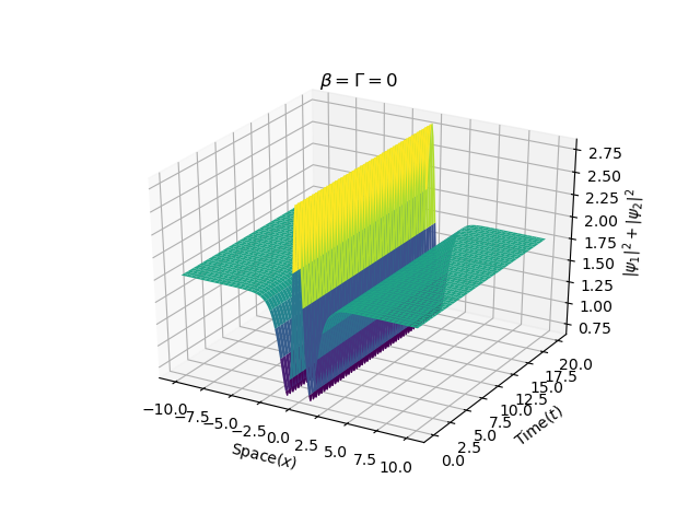
(a)

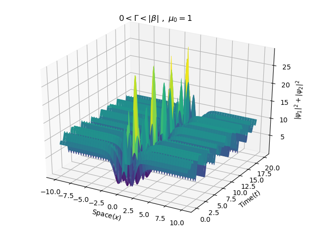
(b)

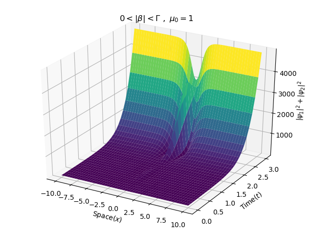
(c)

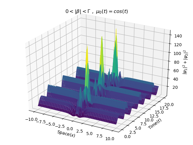
(d)

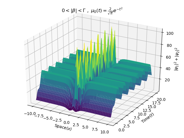
(e)

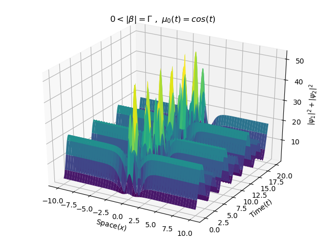
(f)

Figure 1: (Color online) Plot of $|\psi_{1}|^{2}+|\psi_{2}|^{2}$ of example-I for the parametric value $\theta_{\beta}=\frac{\pi}{3}$, $\theta_{\alpha}=\frac{\pi}{6}$, $\omega_{1}=2$, $\omega_{2}=-2$, $\Omega=1$ and $\delta=0$. In Fig(a): $\Gamma=|\beta|=0,A=2.121,B=2.121$, Fig(b): $\Gamma=1.5,|\beta|=2,\mu_{0}=1,A=3.674,B=1.643$, Fig(c): $\Gamma=2.3,|\beta|=2,\mu_{0}=1,A=2.822,B=1.771$, Fig(d): $\Gamma=2.3,|\beta|=2,\mu_{0}(t)=cos(t),A=2.822,B=1.771$, Fig(e): $\Gamma=2.3,|\beta|=2,\mu_{0}(t)=\frac{2}{\sqrt{\pi}}e^{-t^{2}},A=2.822,B=1.771$, Fig(f): $\Gamma=|\beta|=2,\mu_{0}(t)=cos(t),A=3,B=1.732$

Figure. 1 shows the power $P=|\psi_{1}|^{2}+|\psi_{2}|^{2}$ plotted, for various time-modulations. Fig. 1(a) depicts the scenario when BLG and LC vanish, and there is no change in the power over time. For constatnt $\mu_{0}$ and a non-vanishing $\beta$,$\Gamma$, fulfilling $|\beta|>\Gamma$, the power-oscillation can be shown in Fig. 1(b). The power oscillation in time is the signature of the balanced loss-gain system. The solution $\Psi$ becomes unstable for constant $\mu_{0}$ and non-vanishing $\beta$,  $\Gamma$ while satisfying $|\beta|\leq\Gamma$. The relevant plot is displayed in Fig. 1.(c). It may be recalled from our earlier discussions in Sec. 3 that the transformation (25) that joins the initial system given by Eq. (2) to Eq. (29), does not change the stability property of $\Phi(x,t)$ for a bounded U(t). Thus, for a given stable solution of Eq. (29), the solutions of Eq. (2) are stable for bounded $U(t)$, i.e. suitable choice of $\mu_{0}(t)$. We can control the instability by wisely selecting $\mu_{0}(t)$. We have taken into account $|\beta|<\Gamma$ and a periodic modulation function $\mu_{0}(t)=cos(t)$ for which $P(x,t)$ exhibits periodic behaviour in Fig. 1(d). In Fig. 1(e), which is likewise time-bounded, we have plotted power for the conditions $|\beta|<\Gamma$ and $\mu_{0}(t)=\frac{2}{\sqrt{\pi}}e^{-t^{2}}$. The instability in the region $|\beta|=\Gamma$ may once more be controlled using periodic time moduation. The plot in Fig. 1(f) in particular displays power oscillation for $\mu_{0}(t)=cos(t)$ in the region $|\beta|=\Gamma$ . The mentioned features have been verified up to time $t\approx 200$, although the figures are only displayed up to time $t\approx 20$.

Example-II: We present the bright-dark soliton solution of Eq. (38) with $V(x)=0$ corresponding to the Solution VIII in Ref. [25],

$$Q_{1}(x,t)=A\operatorname{sech}\left(\Omega x\right)e^{-i\left(\omega_{1}t+\delta\right)},\ \ Q_{2}(x,t)=B\tanh\left(\Omega x\right)e^{-i\left(\omega_{2}t+\delta\right)},$$

$$\Omega^{2}=-\frac{1}{2}(\lambda_{+}A^{2}+\lambda_{-}B^{2}),$$

$$\omega_{1}=\Omega^{2}+\lambda_{+}A^{2},\ \ \omega_{2}=\Omega^{2}+\omega_{1}$$ (42)

where $A$ and $B$ denote the amplitudes. The positivity of $\Omega^{2}$ is ensured when $\frac{B^{2}-A^{2}}{B^{2}+A^{2}}>\frac{|\beta|}{\Gamma}\ \sin(\theta_{\alpha}-\theta_{\beta})$. The solution of Eq. (1) is,

$$\psi_{1}(x,t) = \frac{1}{\sqrt{2}}\ \left[\left\{cos(\epsilon)+(\Gamma-i\beta^{*}e^{i\theta_{\alpha}})\frac{\sin(\epsilon)}{\epsilon_{0}}\right\}A\ \operatorname{sech}(\Omega x)\ e^{-i(\omega_{1}t+\delta)}\right.$$

$$+ \left.\left\{-e^{-i\theta_{\alpha}}\cos(\epsilon)-(\Gamma e^{-i\theta_{\alpha}}+i\beta^{*})\frac{\sin(\epsilon)}{\epsilon_{0}}\right\}\ B\ \tanh(\Omega x)\ e^{-i(\omega_{2}t+\delta)}\right]$$

$$\psi_{2}(x,t) = \frac{1}{\sqrt{2}}\ \left[\left\{cos(\epsilon)-(\Gamma-i\beta e^{-i\theta_{\alpha}})\frac{\sin(\epsilon)}{\epsilon_{0}}\right\}B\ \tanh(\Omega x)\ e^{-i(\omega_{2}t+\delta)}\right.$$ (43)

$$+ \left.\left\{e^{i\theta_{\alpha}}\cos(\epsilon)-(\Gamma e^{i\theta_{\alpha}}+i\beta)\frac{\sin(\epsilon)}{\epsilon_{0}}\right\}A\ \operatorname{sech}(\Omega x)\ e^{-i(\omega_{1}t+\delta)}\right]$$

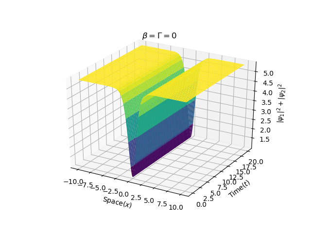
(a)

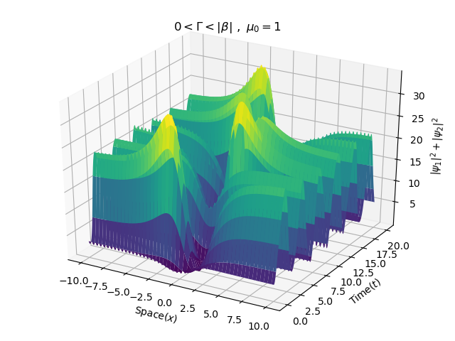
(b)

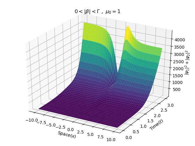
(c)

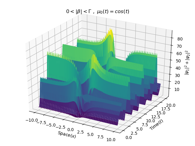
(d)

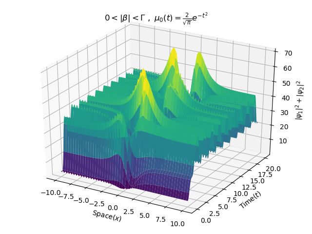
(e)

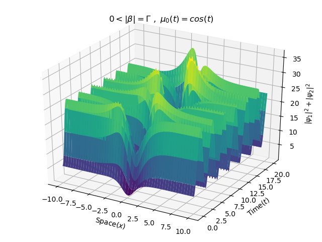
(f)

Figure 2: (Color online) Plot of $|\psi_{1}|^{2}+|\psi_{2}|^{2}$ of example-II for the parametric value $A=1$, $B=\sqrt{\frac{27}{5}}$, $\theta_{\beta}=\frac{\pi}{6}$, $\theta_{\alpha}=\frac{\pi}{3}$ and $\delta=0$. In Fig(a): $\Gamma=|\beta|=0,\omega_{1}=3.2,\omega_{2}=5.4,\Omega=2.2$, Fig(b): $\Gamma=1.5,|\beta|=2,\mu_{0}=1,\omega_{1}=1.957,\omega_{2}=2.349,\Omega=0.626$, Fig(c): $\Gamma=2.3,|\beta|=2,\mu_{0}=1,\omega_{1}=2.243,\omega_{2}=3.052,\Omega=0.899$, Fig(d): $\Gamma=2.3,|\beta|=2,\mu_{0}(t)=cos(t),\omega_{1}=2.243,\omega_{2}=3.052,\Omega=0.899$, Fig(e): $\Gamma=2.3,|\beta|=2,\mu_{0}(t)=\frac{2}{\sqrt{\pi}}e^{-t^{2}},\omega_{1}=2.243,\omega_{2}=3.052,\Omega=0.899$, Fig(f) : $\Gamma=|\beta|=2,\mu_{0}(t)=cos(t),\omega_{1}=2.1,\omega_{2}=2.7,\Omega=0.774$

The qualitative behaviour of the plots in Figure (2) under the same circumstances on $\beta,\Gamma$ and $\mu_{0}(t)$ is identical to that of Fig. 1. The power oscillation is absent for vanishing $\beta,\Gamma$ as shown in Fig. 2(a). Fig. 2(b) depicts the power-oscillation for constant $\mu_{0}$ and $|\beta|>\Gamma$. As seen in Fig. 2(c), the solution expands with no upper bound for constants $\mu_{0}$ and $|\beta|<\Gamma$. Figs. 2(d), 2(e), and 2(f) illustrate how instabilities for $|\beta|\leq\Gamma$ are managed by selecting an appropriate $\mu_{0}(t)$.

3.1.2 Non-vanishing confining potential

We have presented two solutions of Eq. (38) for a special case $V(x,t)=0$. Several solutions of Eq. (38) with $\cal{PT}$-symmetric confining potential can be constructed. The solution of Eq. (38) with $V(x,t)=S(x)+i\tilde{S}(x)$ can be written as,

$$Q_{1}(x,t) = W_{1}\ q(x)\ e^{i\big{(}r(x)+\omega t+\theta_{1}\big{)}}$$

$$Q_{2}(x,t) = W_{2}\ q(x)\ e^{i\big{(}r(x)+\omega t+\theta_{2}\big{)}}$$ (44)

where $q(x)$ and $r(x)$ are real function and denote the amplitude and phase respectively. We substitute Eq. (44) into Eq. (38) and the amplitude and phase satisfy the relations

$$S(x) = -\omega+\frac{q_{xx}}{q}-r^{2}_{x}-\alpha\ q(x)\ q(-x)\ \cos(y(x))$$

$$\tilde{S}(x) = r_{xx}+\frac{2q_{x}r_{x}}{q}-\alpha\ q(x)\ q(-x)\ \sin(y(x))$$ (45)

where $y(x)=r(x)-r(-x)$ and the constant $\alpha=\lambda_{+}|W_{1}|^{2}+\lambda_{-}|W_{2}|^{2}$. The solution of Eq. (45) for different kinds of $\cal{PT}$-symmetric potential is discussed in Ref. [30]. The exact solutions of Eq. (6) with $V(x,t)=S(x)+i\tilde{S}(x)$ can be constructed corresponding to each of these solutions by using the relation $\Psi=U\bar{S}Wq(x)e^{i\big{(}r(x)+\omega t\big{)}}$ where the column matrix $W=\Big{(}W_{1}e^{i\theta_{1}}\ \ W_{2}e^{i\theta_{2}}\Big{)}^{T}$.

Generalised Rosen-Morse Potential: We first consider $\cal{PT}$-symmetric generalised complex Rosen-Morse Potential $S(x)+i\tilde{S}(x)$ with the components

$$S(x) = -2\operatorname{sech}^{2}(x)-\alpha a^{2}\operatorname{sech}^{2}(x)\cos(y(x))$$

$$\tilde{S}(x) = -2b\tanh(x)-\alpha a^{2}\operatorname{sech}^{2}(x)\sin(y(x))$$ (46)

where $y(x)=2bx$ and $a,b$ are constant. The solution of Eq. (38) corresponding to this potential is

$$Q(x,t)=\begin{bmatrix}W_{1}e^{i\theta_{1}}\\ W_{2}e^{i\theta_{2}}\end{bmatrix}\ a\operatorname{sech}(x)\ e^{i\big{(}bx+(1-b^{2})t\big{)}}$$ (47)

We can choose appropriate physically motivated $\mu_{0}(t)$ so that $U(t)$ is bounded. We present the solution of Eq. (1) for this generalised Rosen-Morse potential and for a given $\mu_{0}(t)$.

$$\psi_{1}(x,t) = \frac{1}{\sqrt{2}}\ \big{[}\{cos(\epsilon)+(\Gamma-i\beta^{*}e^{i\theta_{\alpha}})\frac{\sin(\epsilon)}{\epsilon_{0}}\}W_{1}\ e^{i\theta_{1}}$$

$$+ \{-e^{-i\theta_{\alpha}}\cos(\epsilon)-(\Gamma e^{-i\theta_{\alpha}}+i\beta^{*})\frac{\sin(\epsilon)}{\epsilon_{0}}\}W_{2}\ e^{i\theta_{2}}\big{]}$$

$$\times\ a\operatorname{sech}(x)\ e^{i\big{(}bx+(1-b^{2})t\big{)}}$$

$$\psi_{2}(x,t) = \frac{1}{\sqrt{2}}\ \big{[}\{\cos(\epsilon)-(\Gamma-i\beta e^{-i\theta_{\alpha}})\frac{\sin(\epsilon)}{\epsilon_{0}}\}W_{2}\ e^{i\theta_{2}}$$ (48)

$$+ \{e^{i\theta_{\alpha}}\cos(\epsilon)-(\Gamma e^{i\theta_{\alpha}}+i\beta)\frac{\sin(\epsilon)}{\epsilon_{0}}\}W_{1}\ e^{i\theta_{1}}\big{]}$$

$$\times\ a\operatorname{sech}(x)\ e^{i\big{(}bx+(1-b^{2})t\big{)}}$$

Generalised Scarf-II potential: We consider $\cal{PT}$-symmetric generalised Scarf-II potential. The real and imaginary parts of the potential are,

$$S(x) = -(2+b^{2})\operatorname{sech}^{2}(x)-\alpha a^{2}\operatorname{sech}^{2}(x)\cos(y(x))$$

$$\tilde{S}(x) = -3b\operatorname{sech}(x)\tanh(x)-\alpha a^{2}\operatorname{sech}^{2}(x)\sin(y(x))$$ (49)

where $y(x)=2b\arctan[\sinh(x)]$ and $a,b$ are constant. The solution of Eq. (38) corresponding to this potential

$$Q(x,t)=\begin{bmatrix}W_{1}e^{i\theta_{1}}\\ W_{2}e^{i\theta_{2}}\end{bmatrix}\ a\operatorname{sech}(x)\ e^{i\big{(}b\arctan[\sinh(x)]+t\big{)}}$$ (50)

We present the solution of Eq. (1) for this generalised Scarf-II potential and for a given $\mu_{0}(t)$.

$$\psi_{1}(x,t) = \frac{1}{\sqrt{2}}\ \big{[}\{cos(\epsilon)+(\Gamma-i\beta^{*}e^{i\theta_{\alpha}})\frac{\sin(\epsilon)}{\epsilon_{0}}\}W_{1}\ e^{i\theta_{1}}$$

$$+ \{-e^{-i\theta_{\alpha}}\cos(\epsilon)-(\Gamma e^{-i\theta_{\alpha}}+i\beta^{*})\frac{\sin(\epsilon)}{\epsilon_{0}}\}W_{2}\ e^{i\theta_{2}}\big{]}$$

$$\times\ a\operatorname{sech}(x)\ e^{i\big{(}b\arctan[\sinh(x)]+t\big{)}}$$

$$\psi_{2}(x,t) = \frac{1}{\sqrt{2}}\ \big{[}\{\cos(\epsilon)-(\Gamma-i\beta e^{-i\theta_{\alpha}})\frac{\sin(\epsilon)}{\epsilon_{0}}\}W_{2}\ e^{i\theta_{2}}$$ (51)

$$+ \{e^{i\theta_{\alpha}}\cos(\epsilon)-(\Gamma e^{i\theta_{\alpha}}+i\beta)\frac{\sin(\epsilon)}{\epsilon_{0}}\}W_{1}\ e^{i\theta_{1}}\big{]}$$

$$\times\ a\operatorname{sech}(x)\ e^{i\big{(}b\arctan[\sinh(x)]+t\big{)}}$$

Periodic Potential: We consider $\cal{PT}$-symmetric generalised periodic potential. The real and imaginary parts of the potential are,

$$S(x) = -b^{2}\cos^{2}(x)-\alpha a^{2}\cos^{2}(x)\cos(y(x))$$

$$\tilde{S}(x) = -3b\sin(x)-\alpha a^{2}\cos^{2}(x)\sin(y(x))$$ (52)

where $y(x)=2b\sin(x)$ and $a,b$ are constant. The solution of Eq. (38) corresponding to this potential

$$Q(x,t)=\begin{bmatrix}W_{1}e^{i\theta_{1}}\\ W_{2}e^{i\theta_{2}}\end{bmatrix}\ a\cos(x)\ e^{i\big{(}b\sin(x)+t\big{)}}$$ (53)

We present the solution of Eq. (1) for this $\cal{PT}$-symmetric periodic potential and for a given $\mu_{0}(t)$.

$$\psi_{1}(x,t) = \frac{1}{\sqrt{2}}\ \big{[}\{cos(\epsilon)+(\Gamma-i\beta^{*}e^{i\theta_{\alpha}})\frac{\sin(\epsilon)}{\epsilon_{0}}\}W_{1}\ e^{i\theta_{1}}$$

$$+ \{-e^{-i\theta_{\alpha}}\cos(\epsilon)-(\Gamma e^{-i\theta_{\alpha}}+i\beta^{*})\frac{\sin(\epsilon)}{\epsilon_{0}}\}W_{2}\ e^{i\theta_{2}}\big{]}$$

$$\times \ a\cos(x)\ e^{i\big{(}b\sin(x)+t\big{)}}$$

$$\psi_{2}(x,t) = \frac{1}{\sqrt{2}}\ \big{[}\{\cos(\epsilon)-(\Gamma-i\beta e^{-i\theta_{\alpha}})\frac{\sin(\epsilon)}{\epsilon_{0}}\}W_{2}\ e^{i\theta_{2}}$$ (54)

$$+ \{e^{i\theta_{\alpha}}\cos(\epsilon)-(\Gamma e^{i\theta_{\alpha}}+i\beta)\frac{\sin(\epsilon)}{\epsilon_{0}}\}W_{1}\ e^{i\theta_{1}}\big{]}$$

$$\times \ a\cos(x)\ e^{i\big{(}b\sin(x)+t\big{)}}$$

3.2 General Case

To solve the general case i.e $V(x,t)\neq 0$ and $M\neq L$, we consider the solution of Eq. (29) as,

$$\Phi(x,t) = W\rho(x,t)e^{i\eta(x,t)}u(\zeta)\ ;\ \zeta=\zeta(x,t)$$ (55)

where $W=\big{(}W_{1}e^{i\theta_{1}}\ \ W_{2}e^{i\theta_{2}}\big{)}^{T}$ is a constant complex vector and $\zeta(x,t)$ is an odd function under parity transformation i.e. $\zeta(-x,t)=-\zeta(x,t)$. This is an essential condition because our aim is to reduce Eq. (29) into a solvable equation and Eq. (29) reduces to solvable Eq. (68) only when $\zeta(-x,t)$ is an odd function under parity transformation. $\rho(x,t),\zeta(x,t),\eta(x,t)$ and $V(x,t)$ satisfy the following sets of equations

$$\rho\rho_{t}+(\rho^{2}\eta_{x})_{x} = \rho^{2}(x,t)\tilde{S}(x,t)$$ (56)

$$\zeta_{t}(x,t)+2\eta_{x}(x,t)\zeta_{x}(x,t) = 0$$ (57)

$$(\rho^{2}\zeta_{x})_{x} = 0$$ (58)

$$S(x,t) = \frac{\rho_{xx}}{\rho}-\eta_{t}-\eta^{2}_{x}-\mu\zeta^{2}_{x}$$ (59)

where $\mu$ is a constant. This set of equations is same as shown in Ref [21] in the context of one component NNLSE. The ansatz as shown in Eq. (55), was also used in Ref. [67] for one component localized NLSE. Inserting the Eq.( 55) into Eq. (29) we get,

$$u_{\zeta\zeta}+\mu\ u = \frac{1}{W^{\dagger}W}[W^{\dagger}K(l_{11},m_{11})WW^{\dagger}F_{+}W+W^{\dagger}K(l_{22},m_{22})WW^{\dagger}F_{-}W$$ (60)

$$+ W^{\dagger}K(l_{12},m_{12})WW^{\dagger}BW+W^{\dagger}K(l_{21},m_{21})WW^{\dagger}B^{\dagger}W]$$

$$\times \frac{\rho(-x,t)\rho(x,t)}{\zeta^{2}_{x}}\ e^{i(\eta(x,t)-\eta(-x,t))}\ u^{*}(-\zeta)u^{2}(\zeta)$$

The nonlinear term will be real for the judicious choice of $l_{ij}$ and $m_{ij}$. To ensure that the co-efficient of the nonlinear term is real and Eq. (60) reduces to Eq. (67), the following conditions should be satisfied

$$l_{12}=l_{21}\ ;\ m_{12}=m_{21}$$

$$l_{11}+m_{11}=\frac{f_{1}(x,t)}{W^{\dagger}F_{+}W}$$

$$l_{22}+m_{22}=\frac{f_{2}(x,t)}{W^{\dagger}F_{-}W}$$

$$l_{12}+m_{12}=\frac{f_{3}(x,t)}{W^{\dagger}(B+B^{\dagger})W}$$

$$l_{11}-m_{11}=-(l_{22}-m_{12})\frac{W^{\dagger}F_{-}W}{W^{\dagger}F_{+}W}-(l_{12}-m_{12})\frac{W^{\dagger}(B+B^{\dagger})W}{W^{\dagger}F_{+}W}$$ (61)

where $f_{1}(x,t)$,$f_{2}(x,t)$ and $f_{3}(x,t)$ are arbitrary functions. The expressions of space-time modulated strength $l_{ij}$,$m_{ij}$ of nonlinear interaction may be obtained by solving the group of Eqs. (61). We solve the equations by keeping $m_{22}$, $m_{12}$ and $m_{21}$ arbitrary :

$$l_{11} = \frac{1}{2W^{\dagger}F_{+}W}[f_{1}(x,t)-f_{2}(x,t)-f_{3}(x,t)$$

$$+ 2m_{22}W^{\dagger}F_{-}W+2m_{12}W^{\dagger}(B+B^{\dagger})W]$$

$$m_{11} = \frac{1}{2W^{\dagger}F_{+}W}[f_{1}(x,t)+f_{2}(x,t)+f_{3}(x,t)$$

$$- 2m_{22}W^{\dagger}F_{-}W-2m_{12}W^{\dagger}(B+B^{\dagger})W]$$

$$l_{12} = \frac{f_{3}(x,t)}{W^{\dagger}(B+B^{\dagger})W}-m_{12}$$

$$l_{22} = \frac{f_{2}(x,t)}{W^{\dagger}F_{-}W}-m_{22}$$ (62)

The above expressions will be same for both the local and nonlocal cases. For $l_{ij}=m_{ij}=0$ , $i\neq j$ the Eq. (62) reduces to the Eq. (19) of Ref. [49]. The signature of the nonlocality in Eq. (60) is carried by the terms $\rho(-x,t)$, $\eta(-x,t)$ and $u^{*}(-\zeta)$. Instead of the complicated form we choose a simple form of $l_{ij}$, $m_{ij}$ to present our result:

$$l_{11}=\frac{f_{1}(x,t)+G(x,t)}{2W^{\dagger}F_{+}W}\ ;\ m_{11}=\frac{f_{1}(x,t)-G(x,t)}{2W^{\dagger}F_{+}W}$$

$$l_{22}=\frac{f_{2}(x,t)-G(x,t)}{2W^{\dagger}F_{-}W}\ ;\ m_{22}=\frac{f_{2}(x,t)+G(x,t)}{2W^{\dagger}F_{-}W}$$

$$l_{21}=l_{12}=m_{12}=m_{21}=\frac{f_{3}(x,t)}{2W^{\dagger}(B+B^{\dagger})W}$$ (63)

where $G(x,t)$ is an arbitrary function. The choice of $l_{ij}$ and $m_{ij}$ to ensure that the nonlinear term is real, is not unique. There are others choices too. For the time being we are considering the above choices. The expressions for $W^{\dagger}F_{\pm}W$ are

$$W^{\dagger}F_{\pm}W=b_{0}\big{(}\frac{1}{2}+T_{\pm}\mu(t)D\big{)}+b_{3}[\frac{\Gamma\mu(t)}{2\epsilon}\sin(2\epsilon)\pm\frac{1}{2}\cos(2\epsilon)]$$ (64)

where $\beta=|\beta|e^{i\theta_{3}}$ and $b_{j}=W^{\dagger}\sigma_{j}W\ ;\ j=0,1,2,3$. The constant $D$ is defined as,

$$D=\Gamma+\frac{2}{b_{0}}\ W_{1}\ W_{2}|\beta|\sin(\theta_{2}-\theta_{1}-\theta_{3})$$ (65)

Both the expressions of $W^{\dagger}F_{\pm}W$ and $D$ are shown in the Ref.[49] in the context of local NLSE. In both the cases the above expressions are same. Due to the presence of cross terms $l_{ij},m_{ij}$ with $i\neq j$ the terms $W^{\dagger}BW$ and $W^{\dagger}B^{\dagger}W$ have arisen. For the nonlinear term to be real, as we have considered all the cross terms are equal to each other, from the last two terms of the right hand side of Eq. (60) we get,

$$W^{\dagger}K(l_{12},m_{12})W\ W^{\dagger}BW+W^{\dagger}K(l_{21},m_{21})W\ W^{\dagger}B^{\dagger}W=l_{12}b_{0}W^{\dagger}(B+B^{\dagger})W$$

The expression of $W^{\dagger}(B+B^{\dagger})W$ is,

$$W^{\dagger}(B+B^{\dagger})W = 2W_{1}W_{2}\cos(\theta_{1}-\theta_{2})\cos^{2}(\epsilon)+\{2W_{1}W_{2}\big{(}|\beta|^{2}\cos(\theta_{1}-\theta_{2}+2\theta_{3})$$ (66)

$$- \Gamma^{2}\cos(\theta_{1}-\theta_{2})\big{)}+2\Gamma|\beta|\sin(\theta_{3})b_{0}\}\ \frac{\sin^{2}(\epsilon)}{\epsilon^{2}}$$

The imaginary part of the non linear term vanishes for the choice of $l_{ij}$ and $m_{ij}$ as in Eq. (63) and Eq. (60) reduces to the following,

$$u_{\zeta\zeta}+\mu u=f(x,t)\ \frac{\rho(-x,t)\rho(x,t)}{\zeta^{2}_{x}}\ e^{i(\eta(x,t)-\eta(-x,t)}\ u^{*}(-\zeta)u^{2}(\zeta)$$ (67)

and $f(x,t)=\frac{1}{2}[f_{1}(x,t)+f_{2}(x,t)+f_{3}(x,t)]$. Note that Eq. (67) reduces to the following equation

$$u_{\zeta\zeta}+\mu u-2\sigma u^{*}(-\zeta)u^{2}(\zeta)=0$$ (68)

if the following condition is satisfied

$$f(x,t)=\frac{2\sigma\ \zeta^{2}_{x}}{\rho(-x,t)\rho(x,t)}e^{i\big{(}\eta(-x,t)-\eta(x,t)\big{)}}$$ (69)

It is to be noted that $f(x,t)$ is a $\cal{PT}$ symmetric function i.e. $f^{*}(-x,t)=f(x,t)$, since $\zeta(x,t)$ is an odd function of space. Hence $\zeta_{x}(x,t)$ is an even function of space i.e. $\zeta_{x}(-x,t)=\zeta_{x}(x,t)$. The general solution of Eq. (1) can be written as,

$$\psi(x,t)=U(t)\ W\ \rho(x,t)\ u(\zeta)\ e^{i\eta(x,t)}$$ (70)

where $U(t)$ is given in Eq. (26) and $\rho(x,t)$, $\eta(x,t)$, $\zeta(x,t)$ and $u(\zeta)$ are to be determined from Eqs. (57), (58), (59), (68) respectively. Eq. (68) is solvable and has many standard solutions. The solution of Eq. (68) is as follows,

$$u(\zeta)=\sqrt{d_{1}}\ sn\{\sqrt{d_{2}|\sigma|}(\zeta-\zeta_{0}),k\}$$ (71)

where we have considered $\sigma<0$, $\mu>0$ and $u(\zeta)$ is an odd function. Here the constants $d_{1}$ and $d_{2}$ are expressed in terms of constants $m,\sigma,c_{1}$ as shown below,

$$d_{1} = \frac{\mu}{2|\sigma|}-\sqrt{(\frac{\mu}{2|\sigma|})^{2}-\frac{c_{1}}{\sigma}}$$

$$d_{2} = \frac{\mu}{2|\sigma|}+\sqrt{(\frac{\mu}{2|\sigma|})^{2}-\frac{c_{1}}{\sigma}}$$

The expressions of power $P=\Psi^{\dagger}\Psi$ is given as,

$$P(x,t)=P_{1}(t)\rho^{2}(x,t)u^{2}(\zeta),\ P_{1}\equiv W^{\dagger}U^{\dagger}(t)U(t)W$$

The time dependent function $P_{1}(t)$ is determined using the non-unitary matrix $U(t)$ and the expression is given below,

$$P_{1}(t)=b_{0}\ [1+\frac{2\Gamma D}{{\epsilon_{0}}^{2}}\sin^{2}(\epsilon)+\frac{b_{3}\Gamma}{b_{0}\epsilon_{0}}\sin(2\epsilon)]$$ (72)

The expression of $P_{1}(t)$ is independent of local and nonlocal nature of NLSE. This expression is the signature of non-unitary transformation in the expression of power or final solution.

Different Physically motivated examples are presented in Ref.[21] without balanced loss-gain. Those are also applicable here for $\rho(x,t)$, $\zeta(x,t)$, $\eta(x,t)$ for different kinds of potentials and $f(x,t)$. The complete solution of Eq. (1) is obtained by using Eq. (70). Some of the results are presented here in the following tables

Table 1: Examples

	V(x)	f(x)	$\zeta(x)$	Parameters
Sol-I	$E^{2}x^{2}$	$2\sigma\ e^{3Ex^{2}}$	$\sqrt{\frac{\pi}{4E}}\times$	$E>0,\mu=0$
			$erf(\sqrt{E}x)$	$\sigma<0$
Sol-II	$N^{2}-N(N+1)$	$2\sigma\cosh^{6N}(x)$	$\int^{x}\cosh^{2N}(x)dx$	$\mu=0,E=0$
	$\times sech^{2}(x)$			$\sigma<0$
Sol-III	0	$\frac{2\sigma}{\{1+\alpha\cos(\omega x)\}^{3}}$	$\frac{2}{\omega\sqrt{1-\alpha^{2}}}\times\$	$E=\frac{\omega^{2}}{4}>0$
			$\arctan[\frac{\sqrt{1-\alpha}}{\sqrt{1+\alpha}}\tan(\frac{\omega x}{2})]$	$\mu=(1-\alpha^{2})E$

Sol-I:

$$\psi_{1}(x,t) = [W_{1}e^{i\theta_{1}}\cos(\epsilon)-\frac{iW_{2}\beta^{*}}{\epsilon_{0}}e^{i\theta_{2}}\sin(\epsilon)+\frac{\Gamma W_{1}}{\epsilon_{0}}e^{i\theta_{1}}\sin(\epsilon)]$$

$$\times e^{-\frac{1}{2}Ex^{2}}\frac{c}{\sqrt{2|\sigma|}}\ cn(c\zeta,\frac{1}{2})\ e^{-iEt}$$

$$\psi_{2}(x,t) = [W_{2}e^{i\theta_{2}}\cos(\epsilon)-\frac{iW_{1}\beta}{\epsilon_{0}}e^{i\theta_{1}}\sin(\epsilon)-\frac{\Gamma W_{2}}{\epsilon_{0}}e^{i\theta_{2}}\sin(\epsilon)]$$ (73)

$$\times e^{-\frac{1}{2}Ex^{2}}\frac{c}{\sqrt{2|\sigma|}}\ cn(c\zeta,\frac{1}{2})\ e^{-iEt}$$

Sol-II:

$$\psi_{1}(x,t) = [W_{1}e^{i\theta_{1}}\cos(\epsilon)-\frac{iW_{2}\beta^{*}}{\epsilon_{0}}e^{i\theta_{2}}\sin(\epsilon)+\frac{\Gamma W_{1}}{\epsilon_{0}}e^{i\theta_{1}}\sin(\epsilon)]$$

$$\times \operatorname{sech}^{N}(x)\ \frac{c}{\sqrt{2|\sigma|}}\ cn(c\zeta,\frac{1}{2})$$

$$\psi_{2}(x,t) = [W_{2}e^{i\theta_{2}}\cos(\epsilon)-\frac{iW_{1}\beta}{\epsilon_{0}}e^{i\theta_{1}}\sin(\epsilon)-\frac{\Gamma W_{2}}{\epsilon_{0}}e^{i\theta_{2}}\sin(\epsilon)]$$ (74)

$$\times \operatorname{sech}^{N}(x)\ \frac{c}{\sqrt{2|\sigma|}}\ cn(c\zeta,\frac{1}{2})$$

Sol-III:

$$\psi_{1}(x,t) = [W_{1}e^{i\theta_{1}}\cos(\epsilon)-\frac{iW_{2}\beta^{*}}{\epsilon_{0}}e^{i\theta_{2}}\sin(\epsilon)+\frac{\Gamma W_{1}}{\epsilon_{0}}e^{i\theta_{1}}\sin(\epsilon)]$$

$$\times \sqrt{1+\alpha\cos(\omega x)}\ \frac{c}{\sqrt{2|\sigma|}}\sqrt{m}\ sn(c\zeta,m)\ e^{-iEt}\$$

$$\psi_{2}(x,t) = [W_{2}e^{i\theta_{2}}\cos(\epsilon)-\frac{iW_{1}\beta}{\epsilon_{0}}e^{i\theta_{1}}\sin(\epsilon)-\frac{\Gamma W_{2}}{\epsilon_{0}}e^{i\theta_{2}}\sin(\epsilon)]$$ (75)

$$\times \sqrt{1+\alpha\cos(\omega x)}\ \frac{c}{\sqrt{2|\sigma|}}\sqrt{m}\ sn(c\zeta,m)\ e^{-iEt}$$

For Sol-III $\mu=(1+m)c^{2}$ , $|\alpha|<1$ and $\sigma<0$.

All the above solutions are finite in all regions of space. Sol-I and Sol-II are localized in space as $|x|\rightarrow\infty$, amplitude of the solutions tends to zero. With appropriate choice of the parameters, the elliptical functions reduces to hyperbolic function. In this limit, Sol-III also becomes localized. The amplitude of these solutions oscillates with time.

4 Results and Discussions

We have investigated solvable limits of a class of VNNLSE with time dependent BLG and LC terms and space-time modulated nonlinear interaction in presence of confining complex potential. It has been shown that the system admits Lagrangian and Hamiltonian density in a certain limit. In general, the Lagrangian density ${\cal{L}}$ is non-hermitian. Further, it is not equal to its complex conjugate followed by a parity transformation, i. e. ${\cal{L}}(x,t)\neq{\cal{L}}^{\dagger}(-x,t)$, as is the case with the NNLSE or its multi-component and higher dimensional generalizations. The presence of loss-gain terms without the matrix $A$ being $M$-pseudo-hermitian and/or space-time dependence of $M$ is the reason for ${\cal{L}}(x,t)\neq{\cal{L}}^{\dagger}(-x,t)$. The subtleties involved in deriving the Euler-Lagrange equations of motion and conserved Noether charges associated with invariance under continuous symmetry have been discussed. Further, the Hamiltonian, charge, width of the wave packet and its speed of the growth of the system have been shown to be real valued, despite the fact that the corresponding Hamiltonian density, charge density, current density are complex valued. One necessary condition for these dynamical variables to be real valued is that the confining complex potential is $\cal{PT}$-symmetric. The charge has been shown to be a conserved quantity. We have also presented two constants of motion in addition to the Hamiltonian and the charge.

The time-evolution of the system has been studied in terms of certain moments which are analogues of space-integrals of Stokes variables. The VNNLSE can be transformed into a set of linear coupled differential equations satisfied by these moments provided $A$ is $M$-pseudo-hermitian. The resulting equations can be solved exactly if the LC and BLG terms have identical time-modulation. The general method presented in this article for finding solvable limits also requires that the time-modulation of BLG and LC terms are the same. The regions in the parameter-space for bounded and unbounded solutions in time have been identified for time-independent BLG and LC terms. It has been shown that with appropriate choice of time-modulation function $\mu(t)$, the instability in the moments can be tamed. Further, the time-dependence can be tailor-made by suitably choosing $\mu(t)$. This freedom may be utilized in realistic application of the system.

The moment method does not give any expression for the field as a function of space and time. We have adopted a two step approach to find the exact solutions. In the first step, the BLG and LC terms are removed completely by a non-unitary transformation which, in general, modifies the time-modulation of the nonlinear strength. However, in the limit of the loss-gain matrix $A$ being $M$-pseudo-hermitian and the nonlinear interaction is of Manakov-type, i.e. ${|\Psi^{\dagger}(-x.t)M\Psi(x,t)|}^{2}$, the nonlinear term remains invarinat under the transformation. The transformation for this case is identified as pseudo-unitary transformation which is not a symmetry transformation, since it does not preserve the norm. The resulting VNNLSE can be cast into the canonical form of sovable Manakov-type non-local NLSE through an $SU(2)$ rotation. The exact solutions of this equation has been used to find the exact solutions of the system through inverse mapping. Several solutions have been presented for vanishing complex potential. Further, exact solutions of the system are presented for generalized Rosen-Morse, Scarf-II and a complex periodic potential.

The next step is required only if the BLG and LC terms are completely removed by imparting additional time-dependence to the nonlinear strength. The resulting equation for such cases has been mapped to a solvable equation via a co-ordinate transformation. The transformed spatial co-ordinate is necessarily odd under parity transformation. This is to be contrasted with a similar situation in the case of local NLSE where such restriction on the co-ordinate transformation is not required. Several exact solutions have been found. The exact solutions do not depend on specific choices of $f_{1}(x,t)$, $f_{2}(x,t)$, $f_{3}(x,t)$ which appear in the strength of the nonlinear strength, rather depends only on $f(x)=\frac{1}{2}\left[f_{1}(x_{)}+f_{2}(x)+f_{3}(x)\right]$. Several choices of $f_{i}(x)$’s are allowed for a fixed $f(x)$. Further, the exact solution does not depend on the arbitrary function $G(x,t)$ appearing in the nonlinear term. Such a behaviour has been observed for the case of local NLSE also and the possible reason behind this may be attributed to the specific ansatz. The VNNLSE is characterized by the functions $f_{i}(x),i=1,2,3$ and $G(x,t)$ which appear in its nonlinear strength. The fact that the class of solutions presented in this article does not depend on specific form of these functions allows to construct a large number of solvable systems for a fixed $f(x)$. It is desirable that one or more of such solvable VNNLSE may find applications in realistic physical problems. Further, it is expected that the mapping involving pseudo-unitary transformation shall be useful for other nonlinear equations too, albeit with appropriate modifications. This necessitates further investigations involving a variety of nonlinear equations.

5 acknowledgements

SG acknowledges the support of DST INSPIRE fellowship of Govt.of India(Inspire Code No. IF190276).

6 Appendix-I

We have presented two solutions of Eq. (1) with $V(x,t)=0$ and specific choice of $\mu(t)$ in Sec-3.1. The basic method involves mapping Eq. (1) to Eq. (38) whose solutions have been discussed in Ref. [25]. In this appendix, we present other possible solutions of Eq. (1) with $V(x,t)=0$ and any arbitrary $\mu(t)$. It should be noted that all the solutions of Ref. [25] can not be mapped to be exact solutions of Eq. (38), since the parameters $\lambda_{\pm}$ appearing in the latter equation have specific forms and do not satisfy the required conditions. For example, There is no solution of Eq. (38) with $V(x,t)=0$ corresponding to the Solution IV and V in Sec-3 of Ref. [25]. Nevertheless, a large number of solutions can be found. The solutions presented below do not exhaust all the solutions of Ref. [25] which can be mapped to be an exact solutions of Eq. (38), but the complete set of solutions may be found easily.

Solution-III

The solution of Eq. (1) with $V(x,t)=0$ and any arbitrary $\mu(t)$, corresponding to the Solution-I in Ref. [25] is,

$$\psi_{1}(x,t) = \frac{1}{\sqrt{2}}\ \big{[}\{cos(\epsilon)+(\Gamma-i\beta^{*}e^{i\theta_{\alpha}})\frac{\sin(\epsilon)}{\epsilon_{0}}\}Adn(\Omega x,m)e^{-i(\omega_{1}t+\delta_{1})}$$

$$+ \{-e^{-i\theta_{\alpha}}\cos(\epsilon)-(\Gamma e^{-i\theta_{\alpha}}+i\beta^{*})\frac{\sin(\epsilon)}{\epsilon_{0}}\}B\sqrt{m}sn(\Omega x,m)e^{-i(\omega_{2}t+\delta_{2})}\big{]}$$

$$\psi_{2}(x,t) = \frac{1}{\sqrt{2}}\ \big{[}\{\cos(\epsilon)-(\Gamma-i\beta e^{-i\theta_{\alpha}})\frac{\sin(\epsilon)}{\epsilon_{0}}\}B\sqrt{m}sn(\Omega x,m)e^{-i(\omega_{2}t+\delta_{2})}$$ (76)

$$+ \{e^{i\theta_{\alpha}}\cos(\epsilon)-(\Gamma e^{i\theta_{\alpha}}+i\beta)\frac{\sin(\epsilon)}{\epsilon_{0}}\}Adn(\Omega x,m)e^{-i(\omega_{1}t+\delta_{1})}\big{]}$$

provided

$$\lambda_{+}A^{2}+\lambda_{-}B^{2}=-2\Omega^{2}$$ (77)

$$\omega_{1}=m\Omega^{2}+\lambda_{+}A^{2}\ ,\ \omega_{2}=(1+m)\Omega^{2}+\lambda_{+}A^{2}$$ (78)

Solution-IV

The solution of Eq. (1) with $V(x,t)=0$ and any arbitrary $\mu(t)$, corresponding to the Solution-II in Ref. [25] is,

$$\psi_{1}(x,t) = \frac{1}{\sqrt{2}}\ \big{[}\{cos(\epsilon)+(\Gamma-i\beta^{*}e^{i\theta_{\alpha}})\frac{\sin(\epsilon)}{\epsilon_{0}}\}Adn(\Omega x,m)e^{-i(\omega_{1}t+\delta_{1})}$$

$$+ \{-e^{-i\theta_{\alpha}}\cos(\epsilon)-(\Gamma e^{-i\theta_{\alpha}}+i\beta^{*})\frac{\sin(\epsilon)}{\epsilon_{0}}\}B\sqrt{m}cn(\Omega x,m)e^{-i(\omega_{2}t+\delta_{2})}\big{]}$$

$$\psi_{2}(x,t) = \frac{1}{\sqrt{2}}\ \big{[}\{\cos(\epsilon)-(\Gamma-i\beta e^{-i\theta_{\alpha}})\frac{\sin(\epsilon)}{\epsilon_{0}}\}B\sqrt{m}cn(\Omega x,m)e^{-i(\omega_{2}t+\delta_{2})}$$ (79)

$$+ \{e^{i\theta_{\alpha}}\cos(\epsilon)-(\Gamma e^{i\theta_{\alpha}}+i\beta)\frac{\sin(\epsilon)}{\epsilon_{0}}\}Adn(\Omega x,m)e^{-i(\omega_{1}t+\delta_{1})}\big{]}$$

provided the parameters satisfy Eq. (77) and

$$\omega_{1} = -(4-3m)\Omega^{2}+(1-m)\lambda_{+}A^{2}$$

$$\omega_{2} = -(2m-1)\Omega^{2}+(1-m)\lambda_{+}A^{2}$$ (80)

Solution-V

The solution of Eq. (1) with $V(x,t)=0$ and any arbitrary $\mu(t)$, corresponding to the Solution-III in Ref. [25] is,

$$\psi_{1}(x,t) = \frac{1}{\sqrt{2}}\ \big{[}\{cos(\epsilon)+(\Gamma-i\beta^{*}e^{i\theta_{\alpha}})\frac{\sin(\epsilon)}{\epsilon_{0}}\}\{Adn(\Omega x,m)$$

$$+ D\sqrt{m}cn(\Omega x,m)\}e^{-i(\omega_{1}t+\delta_{1})}$$

$$+ \{-e^{-i\theta_{\alpha}}\cos(\epsilon)-(\Gamma e^{-i\theta_{\alpha}}+i\beta^{*})\frac{\sin(\epsilon)}{\epsilon_{0}}\}\{Bdn(\Omega x,m)$$

$$+ E\sqrt{m}cn(\Omega x,m)\}e^{-i(\omega_{2}t+\delta_{2})}\big{]}$$

$$\psi_{2}(x,t) = \frac{1}{\sqrt{2}}\ \big{[}\{\cos(\epsilon)-(\Gamma-i\beta e^{-i\theta_{\alpha}})\frac{\sin(\epsilon)}{\epsilon_{0}}\}\{Bdn(\Omega x,m)$$ (81)

$$+ E\sqrt{m}cn(\Omega x,m)\}e^{-i(\omega_{2}t+\delta_{2})}$$

$$+ \{e^{i\theta_{\alpha}}\cos(\epsilon)-(\Gamma e^{i\theta_{\alpha}}+i\beta)\frac{\sin(\epsilon)}{\epsilon_{0}}\}\{Adn(\Omega x,m)$$

$$+ D\sqrt{m}cn(\Omega x,m)\}e^{-i(\omega_{1}t+\delta_{1})}\big{]}$$

provided the parameters satisfy Eq. (77) and

$$\omega_{1}=\omega_{2}=-\frac{\Omega^{2}}{2}(1+m)\ ,\ D=\pm A\ ,\ E=\pm B$$ (82)

Solution-VI

The solution of Eq. (1) with $V(x,t)=0$ and any arbitrary $\mu(t)$, corresponding to the Solution-VII in Ref. [25] is,

$$\psi_{1}(x,t) = \frac{1}{\sqrt{2}}\ \big{[}\{cos(\epsilon)+(\Gamma-i\beta^{*}e^{i\theta_{\alpha}})\frac{\sin(\epsilon)}{\epsilon_{0}}\}A\sqrt{m}\frac{cn(\Omega x,m)}{dn(\Omega x,m)}e^{-i(\omega_{1}t+\delta_{1})}$$

$$+ \{-e^{-i\theta_{\alpha}}\cos(\epsilon)-(\Gamma e^{-i\theta_{\alpha}}+i\beta^{*})\frac{\sin(\epsilon)}{\epsilon_{0}}\}B\sqrt{m(1-m)}\frac{sn(\Omega x,m)}{dn(\Omega x,m)}e^{-i(\omega_{2}t+\delta_{2})}\big{]}$$

$$\psi_{2}(x,t) = \frac{1}{\sqrt{2}}\ \big{[}\{\cos(\epsilon)-(\Gamma-i\beta e^{-i\theta_{\alpha}})\frac{\sin(\epsilon)}{\epsilon_{0}}\}B\sqrt{m(1-m)}\frac{sn(\Omega x,m)}{dn(\Omega x,m)}e^{-i(\omega_{2}t+\delta_{2})}$$ (83)

$$+ \{e^{i\theta_{\alpha}}\cos(\epsilon)-(\Gamma e^{i\theta_{\alpha}}+i\beta)\frac{\sin(\epsilon)}{\epsilon_{0}}\}A\sqrt{m}\frac{cn(\Omega x,m)}{dn(\Omega x,m)}e^{-i(\omega_{1}t+\delta_{1})}\big{]}$$

provided

$$\lambda_{+}A^{2}+\lambda{-}B^{2}=2\Omega^{2}$$

$$\omega_{1}=(1-m)\Omega^{2}+m\lambda_{+}A^{2}$$

$$\omega_{2}=(1-2m)\Omega^{2}+m\lambda_{+}A^{2}$$ (84)

Solution-VII

The solution of Eq. (1) with $V(x,t)=0$ and any arbitrary $\mu(t)$, corresponding to the Solution-VIII in Ref. [25] is,

$$\psi_{1}(x,t) = \frac{1}{\sqrt{2}}\ \big{[}\{cos(\epsilon)+(\Gamma-i\beta^{*}e^{i\theta_{\alpha}})\frac{\sin(\epsilon)}{\epsilon_{0}}\}A\sqrt{m}\frac{cn(\Omega x,m)}{dn^{2}(\Omega x,m)}e^{-i(\omega_{1}t+\delta_{1})}$$

$$+ \{-e^{-i\theta_{\alpha}}\cos(\epsilon)-(\Gamma e^{-i\theta_{\alpha}}+i\beta^{*})\frac{\sin(\epsilon)}{\epsilon_{0}}\}Bm\frac{cn(\Omega x,m)sn(\Omega x,m)}{dn^{2}(\Omega x,m)}e^{-i(\omega_{2}t+\delta_{2})}\big{]}$$

$$\psi_{2}(x,t) = \frac{1}{\sqrt{2}}\ \big{[}\{\cos(\epsilon)-(\Gamma-i\beta e^{-i\theta_{\alpha}})\frac{\sin(\epsilon)}{\epsilon_{0}}\}Bm\frac{cn(\Omega x,m)sn(\Omega x,m)}{dn^{2}(\Omega x,m)}e^{-i(\omega_{2}t+\delta_{2})}$$ (85)

$$+ \{e^{i\theta_{\alpha}}\cos(\epsilon)-(\Gamma e^{i\theta_{\alpha}}+i\beta)\frac{\sin(\epsilon)}{\epsilon_{0}}\}A\sqrt{m}\frac{cn(\Omega x,m)}{dn^{2}(\Omega x,m)}e^{-i(\omega_{1}t+\delta_{1})}\big{]}$$

provided

$$\omega_{1}=(4m+1)\Omega^{2}\ ,\ \omega_{2}=(4+m)\Omega^{2}$$

$$\lambda_{+}A^{2}=\lambda_{-}B^{2}=6\Omega^{2}$$ (86)

Solution-VIII

The solution of Eq. (1) with $V(x,t)=0$ and any arbitrary $\mu(t)$, corresponding to the Solution-IX in Ref. [25] is,

$$\psi_{1}(x,t) = \frac{1}{\sqrt{2}}\ \big{[}\{cos(\epsilon)+(\Gamma-i\beta^{*}e^{i\theta_{\alpha}})\frac{\sin(\epsilon)}{\epsilon_{0}}\}A\sqrt{m}cn(\Omega x,m)e^{-i(\omega_{1}t+\delta_{1})}$$

$$+ \{-e^{-i\theta_{\alpha}}\cos(\epsilon)-(\Gamma e^{-i\theta_{\alpha}}+i\beta^{*})\frac{\sin(\epsilon)}{\epsilon_{0}}\}B\sqrt{m}sn(\Omega x,m)e^{-i(\omega_{2}t+\delta_{2})}\big{]}$$

$$\psi_{2}(x,t) = \frac{1}{\sqrt{2}}\ \big{[}\{\cos(\epsilon)-(\Gamma-i\beta e^{-i\theta_{\alpha}})\frac{\sin(\epsilon)}{\epsilon_{0}}\}B\sqrt{m}sn(\Omega x,m)e^{-i(\omega_{2}t+\delta_{2})}$$ (87)

$$+ \{e^{i\theta_{\alpha}}\cos(\epsilon)-(\Gamma e^{i\theta_{\alpha}}+i\beta)\frac{\sin(\epsilon)}{\epsilon_{0}}\}A\sqrt{m}cn(\Omega x,m)e^{-i(\omega_{1}t+\delta_{1})}\big{]}$$

provided the parameters satisfy Eq. (77) and

$$\omega_{1}=\Omega^{2}+m\lambda_{+}A^{2}\ ,\ \omega_{2}=m\Omega^{2}+\omega_{1}$$ (88)

Solution-IX

The solution of Eq. (1) with $V(x,t)=0$ and any arbitrary $\mu(t)$, corresponding to the Solution-X in Ref. [25] is,

$$\psi_{1}(x,t) = \frac{1}{\sqrt{2}}\ \big{[}\{cos(\epsilon)+(\Gamma-i\beta^{*}e^{i\theta_{\alpha}})\frac{\sin(\epsilon)}{\epsilon_{0}}\}A\sqrt{m}sn(\Omega x,m)e^{-i(\omega_{1}t+\delta_{1})}$$

$$+ \{-e^{-i\theta_{\alpha}}\cos(\epsilon)-(\Gamma e^{-i\theta_{\alpha}}+i\beta^{*})\frac{\sin(\epsilon)}{\epsilon_{0}}\}B\sqrt{m}sn(\Omega x,m)e^{-i(\omega_{2}t+\delta_{2})}\big{]}$$

$$\psi_{2}(x,t) = \frac{1}{\sqrt{2}}\ \big{[}\{\cos(\epsilon)-(\Gamma-i\beta e^{-i\theta_{\alpha}})\frac{\sin(\epsilon)}{\epsilon_{0}}\}B\sqrt{m}sn(\Omega x,m)e^{-i(\omega_{2}t+\delta_{2})}$$ (89)

$$+ \{e^{i\theta_{\alpha}}\cos(\epsilon)-(\Gamma e^{i\theta_{\alpha}}+i\beta)\frac{\sin(\epsilon)}{\epsilon_{0}}\}A\sqrt{m}sn(\Omega x,m)e^{-i(\omega_{1}t+\delta_{1})}\big{]}$$

provided the parameters satisfy Eq. (77) and

$$\omega_{1}=\omega_{2}=(1+m)\Omega^{2}$$ (90)

Solution-X

The solution of Eq. (1) with $V(x,t)=0$ and any arbitrary $\mu(t)$, corresponding to the Solution-XI in Ref. [25] is,

$$\psi_{1}(x,t) = \frac{1}{\sqrt{2}}\ \big{[}\{cos(\epsilon)+(\Gamma-i\beta^{*}e^{i\theta_{\alpha}})\frac{\sin(\epsilon)}{\epsilon_{0}}\}A\sqrt{m}cn(\Omega x,m)e^{-i(\omega_{1}t+\delta_{1})}$$

$$+ \{-e^{-i\theta_{\alpha}}\cos(\epsilon)-(\Gamma e^{-i\theta_{\alpha}}+i\beta^{*})\frac{\sin(\epsilon)}{\epsilon_{0}}\}B\sqrt{m}cn(\Omega x,m)e^{-i(\omega_{2}t+\delta_{2})}\big{]}$$

$$\psi_{2}(x,t) = \frac{1}{\sqrt{2}}\ \big{[}\{\cos(\epsilon)-(\Gamma-i\beta e^{-i\theta_{\alpha}})\frac{\sin(\epsilon)}{\epsilon_{0}}\}B\sqrt{m}cn(\Omega x,m)e^{-i(\omega_{2}t+\delta_{2})}$$ (91)

$$+ \{e^{i\theta_{\alpha}}\cos(\epsilon)-(\Gamma e^{i\theta_{\alpha}}+i\beta)\frac{\sin(\epsilon)}{\epsilon_{0}}\}A\sqrt{m}cn(\Omega x,m)e^{-i(\omega_{1}t+\delta_{1})}\big{]}$$

provided the parameters satisfy Eq. (77) and

$$\omega_{1}=\omega_{2}=-(2m-1)\Omega^{2}$$ (92)

Solution-XI

The solution of Eq. (1) with $V(x,t)=0$ and any arbitrary $\mu(t)$, corresponding to the Solution-XII in Ref. [25] is,

$$\psi_{1}(x,t) = \frac{1}{\sqrt{2}}\ \big{[}\{cos(\epsilon)+(\Gamma-i\beta^{*}e^{i\theta_{\alpha}})\frac{\sin(\epsilon)}{\epsilon_{0}}\}A\sqrt{m}dn(\Omega x,m)e^{-i(\omega_{1}t+\delta_{1})}$$

$$+ \{-e^{-i\theta_{\alpha}}\cos(\epsilon)-(\Gamma e^{-i\theta_{\alpha}}+i\beta^{*})\frac{\sin(\epsilon)}{\epsilon_{0}}\}B\sqrt{m}dn(\Omega x,m)e^{-i(\omega_{2}t+\delta_{2})}\big{]}$$

$$\psi_{2}(x,t) = \frac{1}{\sqrt{2}}\ \big{[}\{\cos(\epsilon)-(\Gamma-i\beta e^{-i\theta_{\alpha}})\frac{\sin(\epsilon)}{\epsilon_{0}}\}B\sqrt{m}dn(\Omega x,m)e^{-i(\omega_{2}t+\delta_{2})}$$ (93)

$$+ \{e^{i\theta_{\alpha}}\cos(\epsilon)-(\Gamma e^{i\theta_{\alpha}}+i\beta)\frac{\sin(\epsilon)}{\epsilon_{0}}\}A\sqrt{m}dn(\Omega x,m)e^{-i(\omega_{1}t+\delta_{1})}\big{]}$$

provided the parameters satisfy Eq. (77) and

$$\omega_{1}=\omega_{2}=-(2-m)\Omega^{2}$$ (94)

Solution-XII

The solution of Eq. (1) with $V(x,t)=0$ and any arbitrary $\mu(t)$, corresponding to the Solution-XIV in Ref. [25] is,

$$\psi_{1}(x,t) = \frac{1}{\sqrt{2}}\ \big{[}\{cos(\epsilon)+(\Gamma-i\beta^{*}e^{i\theta_{\alpha}})\frac{\sin(\epsilon)}{\epsilon_{0}}\}A\tanh(\Omega x)e^{-i(\omega_{1}t+\delta_{1})}$$

$$+ \{-e^{-i\theta_{\alpha}}\cos(\epsilon)-(\Gamma e^{-i\theta_{\alpha}}+i\beta^{*})\frac{\sin(\epsilon)}{\epsilon_{0}}\}B\tanh(\Omega x)e^{-i(\omega_{2}t+\delta_{2})}\big{]}$$

$$\psi_{2}(x,t) = \frac{1}{\sqrt{2}}\ \big{[}\{\cos(\epsilon)-(\Gamma-i\beta e^{-i\theta_{\alpha}})\frac{\sin(\epsilon)}{\epsilon_{0}}\}B\tanh(\Omega x)e^{-i(\omega_{2}t+\delta_{2})}$$ (95)

$$+ \{e^{i\theta_{\alpha}}\cos(\epsilon)-(\Gamma e^{i\theta_{\alpha}}+i\beta)\frac{\sin(\epsilon)}{\epsilon_{0}}\}A\tanh(\Omega x)e^{-i(\omega_{1}t+\delta_{1})}\big{]}$$

provided the parameters satisfy Eq. (77) and

$$\omega_{1}=\omega_{2}=2\Omega^{2}$$ (96)

Solution-XIV

The solution of Eq. (1) with $V(x,t)=0$ and any arbitrary $\mu(t)$, corresponding to the Solution-XV in Ref. [25] is,

$$\psi_{1}(x,t) = \frac{1}{\sqrt{2}}\ \big{[}\{cos(\epsilon)+(\Gamma-i\beta^{*}e^{i\theta_{\alpha}})\frac{\sin(\epsilon)}{\epsilon_{0}}\}A\operatorname{sech}(\Omega x)e^{-i(\omega_{1}t+\delta_{1})}$$

$$+ \{-e^{-i\theta_{\alpha}}\cos(\epsilon)-(\Gamma e^{-i\theta_{\alpha}}+i\beta^{*})\frac{\sin(\epsilon)}{\epsilon_{0}}\}B\operatorname{sech}(\Omega x)e^{-i(\omega_{2}t+\delta_{2})}\big{]}$$

$$\psi_{2}(x,t) = \frac{1}{\sqrt{2}}\ \big{[}\{\cos(\epsilon)-(\Gamma-i\beta e^{-i\theta_{\alpha}})\frac{\sin(\epsilon)}{\epsilon_{0}}\}B\operatorname{sech}(\Omega x)e^{-i(\omega_{2}t+\delta_{2})}$$ (97)

$$+ \{e^{i\theta_{\alpha}}\cos(\epsilon)-(\Gamma e^{i\theta_{\alpha}}+i\beta)\frac{\sin(\epsilon)}{\epsilon_{0}}\}A\operatorname{sech}(\Omega x)e^{-i(\omega_{1}t+\delta_{1})}\big{]}$$

provided the parameters satisfy Eq. (77) and

$$\omega_{1}=\omega_{2}=-2\Omega^{2}$$ (98)

Solution-XV

The solution of Eq. (1) with $V(x,t)=0$ and any arbitrary $\mu(t)$, corresponding to the Solution-XXII in Ref. [25] is

$$\psi_{1}(x,t) = \frac{1}{\sqrt{2}}\ \big{[}\{cos(\epsilon)+(\Gamma-i\beta^{*}e^{i\theta_{\alpha}})\frac{\sin(\epsilon)}{\epsilon_{0}}\}\{A\operatorname{sech}^{2}(\Omega x)+D\}e^{-i(\omega_{1}t+\delta_{1})}$$

$$+ \{-e^{-i\theta_{\alpha}}\cos(\epsilon)-(\Gamma e^{-i\theta_{\alpha}}+i\beta^{*})\frac{\sin(\epsilon)}{\epsilon_{0}}\}B\tanh(\Omega x)\operatorname{sech}(\Omega x)e^{-i(\omega_{2}t+\delta_{2})}\big{]}$$

$$\psi_{2}(x,t) = \frac{1}{\sqrt{2}}\ \big{[}\{\cos(\epsilon)-(\Gamma-i\beta e^{-i\theta_{\alpha}})\frac{\sin(\epsilon)}{\epsilon_{0}}\}B\tanh(\Omega x)\operatorname{sech}(\Omega x)e^{-i(\omega_{2}t+\delta_{2})}$$ (99)

$$+ \{e^{i\theta_{\alpha}}\cos(\epsilon)-(\Gamma e^{i\theta_{\alpha}}+i\beta)\frac{\sin(\epsilon)}{\epsilon_{0}}\}\{A\operatorname{sech}^{2}(\Omega x)+D\}e^{-i(\omega_{1}t+\delta_{1})}\big{]}$$

provided

$$\lambda_{+}A^{2}=-\lambda_{-}B^{2}=18\Omega^{2}$$

$$\omega_{1}=8\Omega^{2}\ ,\ \omega_{2}=7\Omega^{2}\ ,\ \frac{D}{A}=-\frac{2}{3}$$ (100)

References

• [1] Y. Kivshar and G. P. Agrawal, Optical Solitons: From fibers to Photonic crystals (Academic Press, 2003).
• [2] V. N. Serkin and A. Hasegawa, Novel Soliton Solutions of the Nonlinear Schr$\ddot{o}$dinger Equation Model, Phys. Rev. Lett. 85, 4502 (2000).
• [3] V. N. Serkin, A. Hasegawa, and T. L. Belyaeva, Non autonomous Solitons in External Potentials, Phys. Rev. Lett. 98, 074102 (2007).
• [4] F. Dalfovo, S. Giorgini, L. P. Pitaevskii, and S. Stringari, Theory of Bose-Einstein condensation in trapped gases, Rev. Mod. Phys. 71, 463 (1999).
• [5] P. G. Kevrekidis, D. J. Frantzeskakis, and R. Carretero-González, Editors, Emergent Nonlinear Phenomena in Bose-Einstein Condensates: Theory and Experiment (Springer, Vol. 45, 2008).
• [6] L. P. Pitaevskii and S. Stringari, Bose-Einstein Condensation, (Oxford University Press, Oxford, 2003).
• [7] E. Kengne, W. Liu, and B. A. Malomed, Spatiotemporal engineering of matter-wave solitons in Bose–Einstein condensates, Phy. Rep. 899,1 (2021).
• [8] K. Trulsen and K. B. Dysthe, A modified nonlinear Schr$\ddot{o}$dinger equation for broader bandwidth gravity waves on deep water , Wave motion 24, 281 (1996).
• [9] R. K. Dodd, J. C. Eilbeck, J. D. Gibbon, and H. C. Morris, Solitons and nonlinear wave equations (Academic Press, New York, 1982).
• [10] A. S. Davydov, Solitons in Molecular Systems (Reidel, Dordrecht, 1985).
• [11] K. Goral, K. Rzazewski, and T. Pfau, Bose-Einstein condensation with magnetic dipole-dipole forces, Phys. Rev. A 61, 051601 (2000).
• [12] A. Griesmaier, J. Werner, S. Hensler, J. Stuhler, and T. Pfau, Bose-Einstein Condensation of Chromium, Phys. Rev. Lett. 94, 160401 (2005).
• [13] A. C. Tam and W. Happer, Long-Range Interactions between cw Self-Focused Laser Beams in an Atomic Vapore, Phys. Rev. Lett. 38, 278 (1977).
• [14] D. Suter and T. Blasberg, Stabilization of transverse solitary waves by a nonlocal response of the nonlinear medium, Phys. Rev. A 48, 4583 (1993).
• [15] T. Pertsch, U. Peschel, J. Kobelke, K. Schuster, H. Bartelt, S. Nolte, A. Tunnermann, and F. Lederer, Nonlinearity and Disorder in Fiber Arrays, Phys. Rev. Lett. 93, 053901 (2004).
• [16] C. Conti, M. Peccianti, and G. Assanto,Observation of Optical Spatial Solitons in a Highly Nonlocal Medium, Phys. Rev. Lett. 92, 113902 (2004).
• [17] M.J. Ablowitz and Z.H. Musslimani, Integrable nonlocal nonlinear Schr$\ddot{o}$dinger equation, Phys. Rev. Lett. 110, 064105 (2013).
• [18] A.K. Sarma, M.A. Miri, Z.H. Musslimani, and D.N. Christodoulides, Continuous and discrete Schr$\ddot{o}$dinger systems with parity-time-symmetric nonlinearities, Phys. Rev. E 89, 052918 (2014).
• [19] D. Sinha and P. K. Ghosh, Integrable nonlocal vector nonlinear Schr$\ddot{o}$dinger equation with self-induced parity-time-symmetric potential, Phys. Lett. A 381, 124 (2017).
• [20] M.J. Ablowitz, Z.H. Musslimani, Integrable discrete PT-symmetric model, Phys. Rev. E 90, 032912 (2014).
• [21] D. Sinha and P. K. Ghosh, Symmetries and exact solutions of a class of nonlocal nonlinear Schrödinger equations with self-induced parity-time-symmetric potential, Physical Review E 91, 042908 (2015).
• [22] T.A. Gadzhimuradov, and A.M. Agalarov, Towards a gauge-equivalent magnetic structure of the nonlocal nonlinear Schr$\ddot{o}$dinger equation, Phys. Rev. A 93, 062124 (2016).
• [23] J. Yang, Physically significant nonlocal nonlinear Schrödinger equation and its soliton solutions, Phys. Rev. E 98, 042202 (2018).
• [24] M. Lakshmanan, Continuum spin system as an exactly solvable dynamical system, Phys. Lett. A 61, 53 (1977).
• [25] A. Khare, and A. Saxena, Periodic and hyperbolic soliton solutions of a number of nonlocal nonlinear equations, J. Math. Phys. 56, 032104 (2015).
• [26] M. Li, and T. Xu, Dark and antidark soliton interactions in the nonlocal nonlinear Schr$\ddot{o}$dinger equation with the self-induced parity-time-symmetric potential, Phys. Rev. E 91, 033202 (2015).
• [27] X. Huang, and L. Ling, Soliton solutions for the nonlocal nonlinear Schr$\ddot{o}$dinger equation, Eur. Phys. J. Plus 131, 148 (2016).
• [28] L.Y. Ma, and Z.N. Zhu, N-soliton solution for an integrable nonlocal discrete focusing nonlinear Schr$\ddot{o}$dinger equation, Appl. Math. Lett. 59, 115 (2016).
• [29] L.Y. Ma, and Z.N. Zhu, Nonlocal nonlinear Schr$\ddot{o}$dinger equation and its discrete version: soliton solutions and gauge equivalence, J. Math. Phys. 57, 083507 (2016).
• [30] Z. Wen, and Z. Yan, Solitons and their stability in the nonlocal nonlinear Schr$\ddot{o}$dinger equation with PT-symmetric potentials, Chaos 27, 053105 (2017).
• [31] K. Chen, and D.J. Zhang, Solutions of the nonlocal nonlinear Schr$\ddot{o}$dinger hierarchy via reduction, Appl. Math. Lett. 75, 82 (2018).
• [32] K. Chen, X. Deng, S. Lou, and D.J. Zhan, Solutions of nonlocal equations reduced from the AKNS hierarchy, Stud. Appl. Math. 00, 1 (2018).
• [33] W. Liu, and X. Li, General soliton solutions to a (2+1)-dimensional nonlocal nonlinear Schr$\ddot{o}$dinger equation with zero and nonzero boundary conditions, Nonlinear Dyn. 93, 721 (2018).
• [34] X.Y. Tang, and Z.F. Liang, A general nonlocal nonlinear Schr$\ddot{o}$dinger equation with shifted parity, charge-conjugate and delayed time reversal, Nonlinear Dyn. 92, 815 (2018).
• [35] B. Sun, General soliton solutions to a nonlocal long-wave-short-wave resonance interaction equation with nonzero boundary condition, Nonlinear Dyn. 92, 1369 (2018).
• [36] E. G. Charalampidis, F. Cooper, A. Khare, J. F. Dawson, A. Khare, J. F. Dawson and A. Saxena, Stability of trapped solutions of a nonlinear Schrödinger equation with a nonlocal nonlinear self-interaction potential, J. Phys. A: Math. Theor. 55, 015703 (2022).
• [37] Pijush K. Ghosh, Classical Hamiltonian Systems with balanced loss and gain, J. Phys.: Conf. Ser. 2038, (2021) 012012.
• [38] P. K. Ghosh and P. Roy, On regular and chaotic dynamics of a non-$\mathcal{PT}$-symmetric Hamiltonian system of a coupled Duffing oscillator with balanced loss and gain, J. Phys. A: Math. Theor. 53, 475202 (2020).
• [39] P. Roy and P. K. Ghosh, Complex dynamical properties of coupled Van der Pol–Duffing oscillators with balanced loss and gain, J. Phys. A: Math. Theor. 55, 315701 (2022).
• [40] Yu. V. Bludov, R. Driben, V. V. Konotop, and B. A. Malomed, Instabilities, Solitons and rogue waves in PT-coupled nonlinear waveguides, J. Opt. 15, 064010 (2013).
• [41] R. Driben, and B. A. Malomed, Stability of solitons in parity-time-symmetric couplers, Opt. Lett. 36, 4323 (2011).
• [42] Yu. V. Bludov, V. V. Konotop, and B. A. Malomed, Stable dark solitons in PT-symmetric dual-core waveguides, Phys. Rev. A 87, 013816 (2013).
• [43] I. V. Barashenkov, S. V. Suchkov, A. A. Sukhorukov, S. V. Dmitriev, and Y. S. Kivshar, Breathers in PT-symmetric optical couplers, Physical Review A 86,053809 (2012).
• [44] R. Driben, and B. A. Malomed, Stabilization of solitons in PT models with supersymmetry by periodic management, EPL 96, 51001 (2011).
• [45] C. Kharif, E. Pelinovsky, and A. Slunyaev, Rogue waves in the ocean (Springer, Heidelberg, 2009).
• [46] V. V. Konotop, J. Yang, and D. A. Zezyulin, Nonlinear waves in PT-symmetric systems, Rev. Mod. Phys. 88, 035002 (2016).
• [47] S. V. Suchkov, B. A. Malomed, S. V. Dmitriev, and Y. S. Kivshar, Solitons in a chain of parity-time-invariant dimers, Physical Review E 84, 046609 (2011).
• [48] P. K. Ghosh, Constructing Solvable Models of Vector Non-linear Schr$\ddot{o}$dinger Equation with Balanced Loss and Gain via Non-unitary transformation, Phys. Lett. A 402, 127361 (2021).
• [49] S. Ghosh and P. K. Ghosh, Non-linear Schr$\ddot{o}$dinger equation with time-dependent balanced loss-gain and space-time modulated non-linear interaction, Annals of Physics 454, 169330 (2023).
• [50] D. Sinha, Integrable Local and Non-local Vector Non-linear Schr$\ddot{o}$dinger Equation with Balanced loss and Gain, Physics Letters A 448, 128338 (2022).
• [51] P. K. Ghosh, Conformal symmetry and nonlinear schrödinger equation, Phys. Rev. A65, (2001) 012103; P. K. Ghosh, Explosion-Implosion duality in the Bose-Einstein Condensation, Phys. Lett. A308, (2003) 411; P. K. Ghosh, Exact results on the dynamics of a multicomponent Bose-Einstein condensate, Phys. Rev. A 65, (2002) 053601; T. Tsurumi and M. Wadati, J. Phys. Soc. Jpn. 67, (1998) 93.
• [52] Ali Mostafazadeh, Pseudo-Unitary Operators and Pseudo-Unitary Quantum Dynamics, J. Math.Phys. 45, (2004) 932.
• [53] J. Belmonte-Beitia,V. M. P$\acute{e}$rez-Garc$\acute{i}$a, V. Vekslerchik, and P. J. Torres, Lie Symmetries and Solitons in Nonlinear Systems with Spatially Inhomogeneous Nonlinearities, Phys. Rev. Lett. 98, 064102 (2007).
• [54] R. El-Ganainy, K. G. Makris, D. N. Christodoulides, and Z. H. Musslimani, Theory of coupled optical PT-symmetric structures, Opt. Lett. 32, 2632 (2007).
• [55] K. G. Markis, R. El-Ganainy, D. N. Christodoulides, and Z. H. Musslimani, Beam Dynamics in PT Symmetric Optical Lattices, Phys. Rev. Lett 100, 103904 (2008).
• [56] S. Stalin, M. Senthilvelan, and M. Lakshmanan, Energy-sharing collisions and the dynamics of degenerate solitons in the nonlocal Manakov system, Nonlinear Dyn. 95, 1767 (2019).
• [57] S. V. Manakov, On the theory of two-dimensional stationary self-focusing of electromagnetic waves, Soviet Journal of Experimental and Theoretical Physics 38, 248 (1974).
• [58] V. E. Zakharov and A. B. Shabat, Exact theory of two-dimensional self-focusing and one-dimensional Self-modulation of waves in nonlinear media, Zh. Eksp. Teor. Fiz. 61, 118 (1971).
• [59] J. Alexandre, P. Millington, and D. Seynaeve, Symmetries and conservation laws in non-Hermitian field theories, Phys. Rev. D 96, 065027 (2017).
• [60] P. Millington, Symmetry properties of non-Hermitian ${\cal{PT}}$-symmetric quantum field theories, J. Phys.: Conf. Ser. 1586, 012001 (2020).
• [61] J. Alexandre, P. Millington, and D. Seynaeve, Consistent description of field theories with nonHermitian mass terms, J. Phys.: Conf. Ser. 952, 012012 (2018).
• [62] P. K. Ghosh, Taming Hamiltonian systems with balanced loss and gain via Lorentz interaction : General results and a case study with Landau Hamiltonian, J. Phys. A: Math. Theor. 52, 415202 (2019).
• [63] D. Sinha and P. K. Ghosh, Integrable coupled Li$\acute{e}$nard-type systems with balanced loss and gain, Annals of Physics 400, 109-127 (2019).
• [64] P. K. Ghosh and D. Sinha, Hamiltonian formulation of systems with balanced loss-gain and exactly solvable models, Annals of Physics 388, 276-304 (2018).
• [65] D. Sinha and P. K. Ghosh, $\cal{PT}$-symmetric rational Calogero model with balanced loss and gain, Eur. Phys. J. Plus 132, 460 (2017).
• [66] B. A. Malomed and H. G. Winful, Stable solitons in two-component active systems, Phys. Rev. E 53, 5365 (1996).
• [67] J. Belmonte-Beitia, V. M. P$\acute{e}$rez-Garc$\acute{i}$a, V. Vekslerchik, and V. V. Konotop, Localized nonlinear waves in systems with time and space-modulated nonlinearities, Phys. Rev. Lett. 100, 164102 (2008).