Robust Bond Portfolio Construction
via Convex-Concave Saddle Point Optimization

Abstract

The minimum (worst case) value of a long-only portfolio of bonds, over a convex set of yield curves and spreads, can be estimated by its sensitivities to the points on the yield curve. We show that sensitivity based estimates are conservative, i.e., underestimate the worst case value, and that the exact worst case value can be found by solving a tractable convex optimization problem. We then show how to construct a long-only bond portfolio that includes the worst case value in its objective or as a constraint, using convex-concave saddle point optimization.

1 Introduction

We consider a long-only portfolio of bonds, and address the problem of robust analysis and portfolio construction, under a worst case framework. In this framework we have a set of possible yield curves and bond spreads, and consider the worst change in value of the portfolio over this uncertainty set.

In the analysis problem, considered in §3, we fix the portfolio, and ask what is the worst case change in portfolio value. We observe that this is a convex optimization problem, readily solved using standard frameworks or domain specific languages (DSLs) for convex optimization. We also consider the linearized version of the same problem, where the true portfolio value is replaced with its first order Taylor approximation. This approximation can be interpreted as using standard methods to analyze bond portfolio value using durations. We show that this is also a convex optimization problem, and is always conservative, i.e., predicts more of a decrease in portfolio value than the exact method.

In the robust portfolio construction problem, considered in §4, we seek a portfolio of bonds that minimizes an objective that includes a robustness term, i.e., the worst case change in value of the portfolio over the set of possible yield curves and spreads. We show that this problem, and its linearized version, can be formulated as convex-concave saddle point problems, where we identify the worst case yield and spread and at the same time, the optimal portfolio. One interesting ramification of the convex-concave saddle point formulation is that, unlike in general worst case (minimax) optimization problems, where there are generally multiple worst case parameters, we need to consider only one worst case yield curve and set of bond spreads.

In §5 we show how the convex-concave saddle point problem can be solved by solving one convex optimization problem. This is done using the well known technique of expressing the worst case portfolio value as the optimal value of the dual problem, which converts a min-max problem into a min-min problem which we directly solve. We illustrate the method for a specific case, and in a companion paper [SLB23] explain how the reformulation technique can be automated, using methods due to Juditsky and Nemirovski [JN21]. Using our disciplined saddle point programming framework, we can pose the robust bond portfolio construction problem in just a few lines of simple and natural code, and solve it efficiently.

We present several variations and extensions in §6, including cases where the bond portfolio contains bonds with different base yield curves, per-period compounding is used to value bonds, and a formulation with a robustness constraint as opposed to an objective term.

Identifying the convex-concave structure of the robust bond portfolio construction problem is a novel theoretical contribution, and allows us to use the powerful theory of convex duality to extract insights such as the existence of a single worst case yield curve, or construct a robust bond portfolio. In addition, while this paper was under review the importance of properly managing risk in a bond portfolio became quite apparent with the collapse of Silicon Valley Bank, where a major factor was the bank’s exposure to interest rate risk.

1.1 Previous and related work

Bond portfolio construction and analysis.

Portfolio construction and analysis are well studied problems in finance, however, most of the literature focuses on equity portfolios. These approaches often can not be directly applied to bond portfolios, as there are important differences between the asset classes, such as the finite maturity of bonds. Yet, by making assumptions about the re-investment rate, bond portfolios can be constructed and analyzed via modern portfolio theory (MPT) [Mar52]. For example, assuming that the re-investment rate is given by the current spot rate, standard MPT can be applied to bond portfolios, where the mean and covariance of the bonds can be derived from sample moments or factor models [Puh08]. Similarly, [KK06] use a factor model for the term structure in an MPT setting.

Other approaches for bond portfolio construction that are not based on MPT include exact matching and immunization [EGBG09]. Exact matching is a method for constructing a bond portfolio that minimizes the required investment amount while ensuring that cash flows arising from liabilities are being met. Immunization refers to matching the duration of assets and liabilities, so that the portfolio value is insensitive to (small) changes in interest rates. Both of these problems can be formulated as linear programs and so tractably solved.

Likewise, the factors influencing bond (portfolio) values are well understood, given the practical implications of the problem [FM12, EGBG09]. However, most of the existing literature focuses on parallel shifts in yield curves and spreads, leading to a trivial worst case scenario. Thus the literature is sparse when it comes to robust bond portfolio construction as it relates to possible changes in yield curves and spreads. Instead, most existing work focuses on the problem of robust portfolio construction under parameter uncertainty in an MPT framework (see, e.g., [TK04, KKF14]).

Convex-concave saddle point optimization.

Convex-concave saddle point problems are a class of optimization problems with objective functions which are convex in a subset of the optimization variables, and concave in the remaining variables. The goal in such problems is to find a saddle point, i.e., values of the convex variables that minimize the objective, and values of the concave variables that maximize it. Convex-concave saddle point problems have been studied for decades. Indeed, much of the theory of game theory is based on solving convex-concave saddle point problems, with early descriptions dating back to the 1920s [VN28], and solutions based on solving them as a single convex problem via duality dating back to the 1950s [VNM53]. In their 1983 book, Nemirovski and Yudin [NY83] describe the oracle complexity of first order optimization methods for convex-concave saddle point problems, based on their previous work on the convergence of the gradient method for convex-concave saddle point problems [NY78]. Since then, existing work either requires a specific structure of the problem such as convex and concave variables only being coupled via a bilinear term [BS16], or only under strong assumptions on the functions’ properties [Nem04].

More recently, Juditsky and Nemirovski [JN21] proposed a general framework for solving convex-concave saddle point problems with a particular conic structure as a single convex minimization via dualization. Building on Juditsky and Nemirovski’s work, the authors of this paper developed disciplined saddle programming (DSP) [SLB23]. The associated DSL makes it easy to express a wide class of convex-concave saddle point problems in a natural way; the problem is then transformed to a single convex optimization problem using Juditsky and Nemirovski’s methods. This is analogous to disciplined convex programming (DCP), which makes it easy to specify and solve a wide variety of convex optimization problems [DB16]. The authors’ DSP software package allows our formulation of the robust portfolio construction problem to be specified in just a few lines of clear code.

2 Bond portfolio value

2.1 Yield curve and spreads

A bond is a financial contract that obligates the issuer to make a series of specified payments over time to the bond holder. We let $t=1,\ldots,T$ denote time periods, with $t=0$ representing now. (The periods are usually six months, a typical time between bond coupon payments.) We represent the bond payments as a vector $c\in{\mbox{\bf R}}_{+}^{T}$, where $T$ is the number of periods, and ${\mbox{\bf R}}_{+}$ denotes the set of nonnegative reals. For each $t=1,\ldots,T$, $c_{t}$ is the payment in period $t$ to the bond holder. A bond has a maturity, which is the period of its last payment; for $t$ larger than the maturity, we have $c_{t}=0$. The cash flows $c_{t}$ include coupon payments as well as the payment of the face value at maturity.

We consider a portfolio of $n$ bonds, with quantities (also called holdings) $h=(h_{1},\ldots,h_{n})\in{\mbox{\bf R}}^{n}_{+}$ of each bond, assumed nonnegative (i.e., only long positions). We assume that all bonds in the portfolio mature at or before time period $T$. We first review some basic facts about bonds, for completeness and also to fix our notation.

Each bond has a known cash flow or sequence of payments, given by $c_{i}\in{\mbox{\bf R}}^{T}_{+}$, $i=1,\ldots,n$. We write $c_{i,t}$ to denote the cash flow from bond $i$ in period $t$. We have $c_{i,t}=0$ for $t$ larger than the maturity of bond $i$. We let $p\in{\mbox{\bf R}}_{+}^{n}$ denote the price of the bonds. The portfolio value is $V=p^{T}h$. The bond prices are modeled using a base yield curve and spreads for each bond, explained below.

Yield curve.

The yield curve is denoted by $y\in{\mbox{\bf R}}^{T}$. The yield curve gives the discount of a future payment, i.e., the current value of a payment of $1 received in period $t$, denoted $P_{t}$. These are given by

$$P_{t}=\exp(-ty_{t}),\quad t=1,\ldots,T.$$

We will work with per-period yields, to simplify the formulas, but following convention, we present all final numerical results as annualized. (For example, if the periods represent six months, the associated annualized yields are given by $2y_{t}$.) We use continuous compounding for simplicity of notation, but all our results readily extend to period-wise compounding, where $P_{t}=(1+y_{t})^{-t}$ (see §6).

The yield curve gives the discount of future payments, and captures market expectations with respect to macroeconomic factors, fiscal and monetary policy interactions, and the vulnerability of private consumption to future (unexpected) shocks.

Bond spreads.

Bond $i$ has spread $s_{i}\geq 0$, which means that the bond is priced at its net present value using the yield curve $y+s_{i}\mathbf{1}$, where $\mathbf{1}$ is the vector with all entries one. This is referred to as a ‘parallel shift’ applied to the base yield curve. We will work with per-period spreads, to simplify the formulas, but will give final results as annualized.

The spread captures the uncertainty in the cash flow associated with the bond, such as default or other optionality, which means that we value a payment of $1 from the bond at period $t$ as $\exp(-t(y_{t}+s_{i}))$, which is less than or equal to $P_{t}=\exp(-ty_{t})$. The riskier the bond, the larger the spread, which means future payments are discounted more heavily.

Bond price.

The price of a bond is modeled as the net present value of its cash flow using these discounts,

$$p_{i}=\sum_{t=1}^{T}c_{i,t}\exp(-t(y_{t}+s_{i})),\quad i=1,\ldots,n.$$ (1)

Portfolio value.

The portfolio value can be expressed as

$$V=p^{T}h=\sum_{i=1}^{n}\sum_{t=1}^{T}h_{i}c_{i,t}\exp(-t(y_{t}+s_{i})).$$ (2)

For reasons mentioned below, it will be convenient to work with the log of the portfolio value,

$$\log V=\log\left(\sum_{i=1}^{n}\sum_{t=1}^{T}h_{i}c_{i,t}\exp(-t(y_{t}+s_{i}))\right).$$ (3)

The portfolio value and log portfolio value are functions of the holdings $h$, the yield curve $y$, and the spreads $s$, but we suppress this dependence to keep the notation light. (The cash flows $c_{i,t}$ are fixed and given.)

Convexity properties.

The portfolio value $V$ is a linear function of $h$, the vector of holdings, for fixed yield curve and spreads. If we fix the holdings, $V$ is a convex function of $(y,s)$, the yield curve and spreads [BV04, Chap. 3]. The log value $\log V$ is a concave function of $h$, for fixed $y$ and $s$, since it is a concave function of a linear function. The log value is a convex function of $(y,s)$, for fixed $h$, since it can be expressed as

$$\log V=\log\left(\sum_{i=1}^{n}\sum_{t=1}^{T}\exp(-t(y_{t}+s_{i})+\log h_{i}+\log c_{i,t})\right),$$

which is the log-sum-exp function of an affine function of $(y,s)$ [BV04, §3.1.5]. Thus $\log V$ is a convex-concave function, concave in $h$ and convex in $(y,s)$.

2.2 Change in bond portfolio value

We are interested in the change in portfolio value when the yield curve and spreads change from their current or nominal values $(y^{\mathrm{nom}},s^{\mathrm{nom}})$ to the values $(y,s)$, with the holdings fixed at $h^{\mathrm{nom}}$. We let $V$ denote the portfolio value with yield curve and spreads $(y,s)$, and $V^{\mathrm{nom}}$ the portfolio value with yield curve and spreads $(y^{\mathrm{nom}},s^{\mathrm{nom}})$, both with holdings $h^{\mathrm{nom}}$. The relative or fractional change in value is given by $V/V^{\mathrm{nom}}-1$. It is convenient to work with the change in the log value,

$$\Delta=\log(V/V^{\mathrm{nom}})=\log V-\log V^{\mathrm{nom}}.$$ (4)

The relative change in value can be expressed in terms of the change in log value as $\exp\Delta-1$. Both $\Delta$ and the relative change in value are readily interpreted. For example, $\Delta=-0.15$ means the portfolio value decreases by the factor $\exp(-0.15)=0.861$, i.e., a relative decrease of $13.9\%$.

Since $\log V$ is a convex function of $(y,s)$, $\Delta$ is also a convex function of $(y,s)$.

First order Taylor approximation.

The first order Taylor approximation of change in log value, denoted $\hat{\Delta}$, is

$$\hat{\Delta}=D_{\text{yld}}^{T}(y-y^{\mathrm{nom}})+D_{\text{spr}}^{T}(s-s^{\mathrm{nom}})\approx\Delta,$$ (5)

where

$$D_{\text{yld}}=\left.\left(\nabla_{y}\log V\right)\right\rvert_{y=y^{\mathrm{nom}},\;s=s^{\mathrm{nom}}}\in{\mbox{\bf R}}^{T},\qquad D_{\text{spr}}=\left.\left(\nabla_{s}\log V\right)\right\rvert_{y=y^{\mathrm{nom}},\;s=s^{\mathrm{nom}}}\in{\mbox{\bf R}}^{n}$$

are the gradients of the log value with respect to the yield curve and spreads, respectively, evaluated at the current value $(y^{\mathrm{nom}},s^{\mathrm{nom}})$. These are given by

$$(D_{\text{yld}})_{t} = -(1/V^{\mathrm{nom}})\sum_{i=1}^{n}th^{\mathrm{nom}}_{i}c_{i,t}\exp(-t(y^{\mathrm{nom}}_{t}+s^{\mathrm{nom}}_{i})),$$

$$(D_{\text{spr}})_{i} = -(1/V^{\mathrm{nom}})\sum_{t=1}^{T}th^{\mathrm{nom}}_{i}c_{i,t}\exp(-t(y^{\mathrm{nom}}_{t}+s^{\mathrm{nom}}_{i})).$$

(In the first expression we sum over the bonds, while in the second we sum over the periods.) The affine approximation (5) is very accurate when $(y,s)$ is near $(y^{\mathrm{nom}},s^{\mathrm{nom}})$.

The gradients $D_{\text{yld}}$ and $D_{\text{spr}}$ can be given traditional interpretations. When $n=1$, i.e., the portfolio consists of a single bond, $D_{\text{spr}}$ is the duration of the bond. When $n=1$ and $t$ is one of the 12 Treasury spot maturities, $(D_{\text{spr}})_{t}$ is a key rate duration of the bond. (We use the symbol $D$ since the entries of the gradients can be interpreted as durations.) We refer to the Taylor approximation (5) as the duration based approximation.

A global lower bound.

Since $\Delta$ is a convex function of $(y,s)$, its Taylor approximation $\hat{\Delta}$ is a global lower bound on $\Delta$ (see, e.g., [BV04, §3.1.3]): For any $(y,s)$ we have

$$\hat{\Delta}=D_{\text{yld}}^{T}(y-y^{\mathrm{nom}})+D_{\text{spr}}^{T}(s-s^{\mathrm{nom}})\leq\Delta.$$ (6)

Note that this inequality holds for any $(y,s)$, whereas the approximation (5) is accurate only for $(y,s)$ near $(y^{\mathrm{nom}},s^{\mathrm{nom}})$. Thus the duration based approximation of the change in log portfolio value is conservative; the true change in log value will be larger than the approximated change in log value.

We can easily obtain a bound on the relative change in portfolio value. Exponentiating the inequality (6) and using the inequality $\exp u\geq 1+u$, we have

$$V/V^{\mathrm{nom}}-1=\exp\Delta-1\geq\exp\hat{\Delta}-1\geq\hat{\Delta}.$$

Therefore $\hat{\Delta}$ is also a lower bound on the relative change in portfolio value using the duration based approximation; the actual fractional change in value will always be more (positive) than the prediction.

3 Worst case analysis

In this section we assume the portfolio holdings are known and fixed as $h^{\mathrm{nom}}$, and consider a nonempty compact convex set $\mathcal{U}\subset{\mbox{\bf R}}^{T}\times{\mbox{\bf R}}^{n}$ of possible yield curves and spreads. (We will say more about choices of $\mathcal{U}$ in §3.3.) We define the worst case portfolio value as

$$V^{\mathrm{wc}}=\min_{(y,s)\in\mathcal{U}}V,$$

i.e., the smallest possible portfolio value over the set of possible yield curves and spreads. It will be convenient to work with the worst case (i.e., most negative) change in log portfolio value, defined as

$$\Delta^{\mathrm{wc}}=\min_{(y,s)\in\mathcal{U}}\Delta=\log V^{\mathrm{wc}}-\log V^{\mathrm{nom}}.$$

When $(y^{\mathrm{nom}},s^{\mathrm{nom}})\in\mathcal{U}$, the worst case log value change is nonpositive.

3.1 Worst case analysis problem

We can evaluate $\Delta^{\mathrm{wc}}$ by solving the convex optimization problem

$$\begin{array}[]{ll}\mbox{minimize}&\Delta\\ \mbox{subject to}&(y,s)\in\mathcal{U},\end{array}$$ (7)

with variables $y$ and $s$. The optimal value of this problem is $\Delta^{\mathrm{wc}}$ (from which we can obtain $V^{\mathrm{wc}}$); by solving it, we also find an associated worst case yield curve and spread, which are themselves interesting. We refer to (7) as the worst case analysis problem.

Implications.

One consequence is that we can evaluate $\Delta^{\mathrm{wc}}$ very efficiently using standard methods of convex optimization [BV04]. Depending on the uncertainty set $\mathcal{U}$, the problem (7) can be expressed very compactly and naturally using domain specific languages for convex optimization, such as CVXPY [DB16], CVX [GB14], Convex.jl [UMZ⁺14], or CVXR [FNB20]. Appendix A gives an example illustrating how simple and natural the full CVXPY code to solve the worst case analysis problem is.

Maximum element.

We mention here a special case with a simple analytical solution. The objective $\Delta$ is monotone nonincreasing in its arguments, i.e., increasing any $y_{t}$ or $s_{i}$ reduces the portfolio value. It follows that if $\mathcal{U}$ has a maximum element $(y^{\mathrm{max}},s^{\mathrm{max}})$, i.e.,

$$(y^{\mathrm{max}},s^{\mathrm{max}})\geq(y,s)~{}\mbox{for all}~{}(y,s)\in\mathcal{U}$$

(with the inequality elementwise), then it is the solution of the worst case analysis problem. As a simple example, consider

$$\mathcal{U}=\{(y,u)\mid y^{\mathrm{min}}\leq y\leq y^{\mathrm{max}},~{}s^{\mathrm{min}}\leq s\leq s^{\mathrm{max}}\},$$

i.e., we are given a range of possible values for each point in the yield curve, and for each spread. This uncertainty set, which is a hyper-rectangle or box, has maximum element $(y^{\mathrm{max}},s^{\mathrm{max}})$, which is (obviously) the choice that minimizes portfolio value.

More interesting choices of uncertainty sets do not have a maximum element; for these cases we must numerically solve the worst case analysis problem (7).

3.2 Linearized worst case analysis problem

We can replace the objective in (7) with the lower bound (6) to obtain the linearized worst case portfolio value problem

$$\begin{array}[]{ll}\mbox{minimize}&\hat{\Delta}=D_{\text{yld}}^{T}(y-y^{\mathrm{nom}})+D_{\text{spr}}^{T}(s-s^{\mathrm{nom}})\\ \mbox{subject to}&(y,s)\in\mathcal{U},\end{array}$$ (8)

with variables $y$ and $s$. Here the objective is affine, whereas in (7) the objective is nonlinear (but convex). From the inequality (6), solving this linearized worst case analysis problem gives us a lower bound on $\Delta^{\mathrm{wc}}$, as well as a very good approximation when the changes in yield curve and spreads are not large. We refer to (8) as the linearized worst case analysis problem, and we denote its optimal value, the worst case change in log value predicted by the linearized approximation, by $\hat{\Delta}^{\mathrm{wc}}$. This estimate of $\Delta^{\mathrm{wc}}$ is conservative, i.e., we have $\hat{\Delta}^{\mathrm{wc}}\leq\Delta^{\mathrm{wc}}$. The linearized problem is commonly used in practice, and therefore provides a baseline for comparison.

3.3 Yield/spread uncertainty sets

In this section we describe some possible choices of the yield/spread uncertainty set $\mathcal{U}$, described as a list of constraints. Before getting to specifics, we make some comments about high level methods one might use to construct uncertainty sets.

From all historical data.

Here we construct $\mathcal{U}$ from all historical data. This conservative approach measures the sensitivity of the portfolio to the yield and spread changing to any previous value, or to a value consistent with some model of the past that we build.

From recent historical data.

Here we construct $\mathcal{U}$ from recent historical data, or create a model that places higher weight on recent data. The idea here is to model plausible changes to the yield curve and spreads using a model based on recent historical values.

From forecasts of future values.

Here we construct $\mathcal{U}$ as a forecasted set of possible values over the future, for example a confidence set associated with some predictions.

From current yield and spread estimation error.

Here $\mathcal{U}$ represents the set of possible values of the current yield and spreads, which acknowledges that the current values are only estimates of some true but unknown value. See, for example, [FPY22] for a discussion of yield curve estimation and a method that can provide uncertainty quantification.

3.3.1 Scenarios

Here $\mathcal{U}$ is the convex hull of a set of yield curves and spreads,

$$\mathcal{U}=\mathop{\bf conv}\{(y^{1},s^{1}),\ldots,(y^{K},s^{K})\},$$

which is a polyhedron defined by its vertices. In this case we can think of $(y^{k},s^{k})$ as $K$ economic regimes or scenarios. In the linearized worst case analysis problem, we minimize a linear function over this polyhedron, so there is always a solution at a vertex, i.e., the worst case yield curve and spread is one of our scenarios. In this case we can solve the worst case analysis problem by simply evaluating the portfolio value for each of our scenarios, and taking the smallest value. When using the true portfolio value, however, we must solve the problem numerically, since the worst case scenario need not be on the vertex; it can be a convex combination of multiple vertices.

3.3.2 Confidence ellipsoid

Another natural uncertainty set is based on a vector Gaussian model of $(y,s)$, with mean $\mu\in{\mbox{\bf R}}^{T+n}$ and covariance $\Sigma\in{\mbox{\bf S}}_{++}^{T+n}$, where ${\mbox{\bf S}}_{++}^{k}$ denotes the set of symmetric positive definite $k\times k$ matrices. We take $\mathcal{U}$ as the associated $(1-\alpha)$-confidence ellipsoid,

$$\mathcal{U}=\{(y,s)\mid((y,s)-\mu)^{T}\Sigma^{-1}((y,s)-\mu)\leq F^{-1}(1-\alpha)\},$$

where $F$ is the cumulative distribution function of a $\chi^{2}$ distribution with $T+n$ degrees of freedom.

3.3.3 Factor model

A standard method for describing yield curves and spreads is via a factor model, with

$$(y,s)=Zf+v,$$

where $f\in{\mbox{\bf R}}^{k}$ is a vector of factors that drive yield curves and spreads, and $v$ represents idiosyncratic variation, i.e., not due to the factors. (In a statistical model, the entries of $v$ are assumed to be uncorrelated to each other and the factor $f$.) The matrix $Z\in{\mbox{\bf R}}^{(T+n)\times k}$ gives the factor loadings of the yield curve values and spreads.

Typical factors include treasury yields with various maturities, as well as other economic quantities. A simple factor model for yields can contain only two or three factors, which are the first few principal components of historical yield curves, called level, slope, and curvature [LS91, CP05].

Using a factor model, we can specify $\mathcal{U}$ by giving an uncertainty set $\mathcal{F}\subset{\mbox{\bf R}}^{k}$ for the factors, for example as

$$\mathcal{U}=\{Zf+v\mid f\in\mathcal{F},~{}\|D^{-1}v\|_{2}^{2}\leq 1\},$$

where $D$ is a positive diagonal matrix with its entries giving the idiosyncratic variation of individual yield curve and spread values. We note that while a factor model is typically used to develop a statistical model of the yield curve and spreads, we use it here to define a (deterministic) set of possible values.

3.3.4 Perturbation description

The uncertainty set $\mathcal{U}$ can be described in terms of possible perturbations to the current values $(y^{\mathrm{nom}},s^{\mathrm{nom}})$. We describe this for the yield curve only, but similar ideas can be used to describe the spreads as well. We take $y=y^{\mathrm{nom}}+\delta$, where $\delta\in{\mbox{\bf R}}^{T}$ is the perturbation to the yield curve. We might impose constraints on the perturbations such as

$$\delta^{\mathrm{min}}\leq\delta\leq\delta^{\mathrm{max}},\qquad\sum_{t=1}^{T}\delta^{2}_{t}\leq\kappa,\qquad\sum_{t=1}^{T-1}(\delta_{t+1}-\delta_{t})^{2}\leq\omega,$$ (9)

where $\delta^{\mathrm{min}},\delta^{\mathrm{max}}$, $\kappa$, and $\omega$ are given parameters, and the first inequalities are elementwise. The first constraint limits the perturbation in yield for any $t$; the second limits the mean square perturbation, and the third is a smoothness constraint, which limits the roughness of the yield curve perturbation. This is of course just an example; one could add many further constraints, such as insisting that the perturbed yield have nonnegative slope, is concave, or that the perturbation is plausible under a statistical model of short term changes in yields.

3.3.5 Constraints

We can add any convex constraints in our description of $\mathcal{U}$. For example, we might add the constraints (9) to a factor model, or confidence ellipsoid. As an example of a constraint related to spreads, we can require that the spreads are nonincreasing as a function of the bond rating, i.e., we always have $s_{i}\leq s_{j}$ if bond $i$ has a higher rating than bond $j$. This is a set of linear inequalities on the vector of spreads $s$.

4 Robust portfolio construction

In the worst case analysis problem described in §3, the portfolio is given as $h^{\mathrm{nom}}$. Here we consider the case where the portfolio is to be chosen. We denote the new portfolio as $h$, with $h^{\mathrm{nom}}$ denoting the nominal or current portfolio. Our goal is to choose $h$, which we do by minimizing an objective function, subject to some constraints.

4.1 Nominal portfolio construction problem

We first describe the nominal bond portfolio construction problem. We are given a nominal objective function $\phi:{\mbox{\bf R}}^{n}\to{\mbox{\bf R}}$ which is to be minimized. The nominal objective function might include tracking error against a benchmark, a risk term, and possibly a transaction cost term if the portfolio is to be constructed from the existing portfolio $h^{\mathrm{nom}}$ (see, e.g., [BBD⁺17]). We will assume that the nominal objective function is convex.

We also have a set of portfolio constraints, which we denote as $h\in\mathcal{H}$, where $\mathcal{H}\subset{\mbox{\bf R}}_{+}^{n}$. The constraint set includes the long-only constraint $h\geq 0$, as well as a budget constraint, such as $p^{T}h=p^{T}h^{\mathrm{nom}}$, which states that the new portfolio has the same value as the original one. (This can be extended to take into account transaction costs if needed.) The constraint set $\mathcal{H}$ can include constraints on exposures to regions or sectors, average ratings, duration, a limit on risk, and so on. We will assume that $\mathcal{H}$ is convex. The nominal portfolio construction problem is

$$\begin{array}[]{ll}\mbox{minimize}&\phi(h)\\ \mbox{subject to}&h\in\mathcal{H},\end{array}$$

with variable $h$. This is a convex optimization problem.

4.2 Robust portfolio construction problem

To obtain the robust portfolio construction problem we add one more penalty term to the nominal objective function, which penalizes the worst case change in value over the given uncertainty set $\mathcal{U}$.

The term, which we refer to as the robustness penalty, is $-\lambda\Delta^{\mathrm{wc}}(h)$, where $\lambda>0$ is a parameter used to trade off the nominal objective $\phi$ and the worst case change in log portfolio value $-\Delta^{\mathrm{wc}}(h)$. Here we write the worst case change in log value with argument $h$, to show its dependence on $h$.

We arrive at the optimization problem

$$\begin{array}[]{ll}\mbox{minimize}&\phi(h)-\lambda\Delta^{\mathrm{wc}}(h)\\ \mbox{subject to}&h\in\mathcal{H},\end{array}$$ (10)

with variable $h$. We refer to this as the robust bond portfolio construction problem. The objective is convex since $\phi$ is convex and $\Delta^{\mathrm{wc}}$ is a concave function of $h$. This means that the robust bond portfolio construction problem is convex.

However, the robustness penalty term $-\Delta^{\mathrm{wc}}(h)$ is not directly amenable to standard convex optimization, since it involves a minimization (over $y$ and $s$) itself. We will address the question of how to tractably handle the robustness penalty term below using methods for convex-concave saddle point optimization.

A different framing of the robust bond portfolio construction problem is to minimize $\phi$ subject to a constraint on $\Delta^{\mathrm{wc}}$. This is readily handled, but we defer the discussion to §6.

4.3 Linearized robust portfolio construction problem

As in the worst case analysis problem we can use the linearized approximation of the worst case log value instead of the true log portfolio value, which gives the problem

$$\begin{array}[]{ll}\mbox{minimize}&\phi(h)-\lambda\hat{\Delta}^{\mathrm{wc}}(h)\\ \mbox{subject to}&h\in\mathcal{H},\end{array}$$ (11)

with variable $h$. Here $\hat{\Delta}^{\mathrm{wc}}$ is the worst case change in log portfolio value predicted by the linearized approximation, i.e., the optimal value of (8), as a function of $h$. We note that $\hat{\Delta}^{\mathrm{wc}}$ is, like $\Delta^{\mathrm{wc}}$, a concave function of $h$.

4.4 Convex-concave saddle point formulation

We can write the robust portfolio construction problem (10) as

$$\underset{h\in\mathcal{H}}{\mbox{minimize}}~{}\max_{(y,s)\in\mathcal{U}}~{}\left(\phi(h)-\lambda\Delta(h,y,s)\right).$$ (12)

(Maximizing $-\lambda\Delta(h,y,s)$ over $(y,s)\in\mathcal{U}$ gives $-\lambda\Delta^{\mathrm{wc}}(h)$.) The objective in (12) is convex in $h$ and concave in $(y,u)$, so this is a convex-concave saddle point problem. Replacing $\Delta$ with $\hat{\Delta}$ yields the saddle point version of the linearized robust portfolio construction problem.

Sion’s minimax theorem [Sio58] tells us that if $\mathcal{H}$ is compact, when we reverse the order of the minimization and maximization we obtain the same value, which implies that there exists a saddle point $(h^{\star},y^{\star},s^{\star})$, which satisfies

$$\phi(h^{\star})-\lambda\Delta(h^{\star},y,s)\leq\phi(h^{\star})-\lambda\Delta(h^{\star},y^{\star},s^{\star})\leq\phi(h)-\lambda\Delta(h,y^{\star},s^{\star})$$

for all $h\in\mathcal{H}$ and $(y,s)\in\mathcal{U}$. The left hand inequality shows that $\phi(h^{\star})-\lambda\Delta(h^{\star},y,s)$ is maximized over $(y,s)\in\mathcal{U}$ by $(y^{\star},s^{\star})$; the right hand inequality shows that $\phi(h)-\lambda\Delta(h,y^{\star},s^{\star})$ is minimized over $h\in\mathcal{H}$ by $h^{\star}$. It follows that $\phi(h^{\star})-\lambda\Delta(h^{\star},y^{\star},s^{\star})$ is the optimal value of the robust portfolio construction problem, $h^{\star}$ is an optimal portfolio, and $(y^{\star},s^{\star})$ is a worst case yield curve and spread.

5 Duality based saddle point method

The robust bond portfolio construction problem (12) is convex, but unfortunately not immediately representable in a DSL. In this section we use a well known trick to transform the problem to one that can be handled directly in a DSL. Using duality we will express $\Delta^{\text{wc}}$ as the maximum of a concave function over some variables that lie in a convex set. This method of transforming an inner minimization is not new; it has been used since the 1950s when Von Neumann proved the minimax theorem using strong duality in his work with Morgenstern on game theory [VNM53].

We now describe the dualization method for the case when $\mathcal{U}$ is a polyhedron of the form

$$\mathcal{U}=\{(y,s)\mid A(y,s)\leq b\},$$

with $A\in{\mbox{\bf R}}^{p\times(T+n)}$ and $b\in{\mbox{\bf R}}^{p}$, and the inequality is elementwise, but similar derivations can be carried out for other descriptions of $\mathcal{U}$.

5.1 Dual form of worst case change in log value

We assume Slater’s condition hold, since any uncertainty set in practice will have a nonempty relative interior. From strong duality, it follows that

$$\Delta^{\text{wc}}(h)=\max_{\mu\geq 0,\;\nu}~{}g(h,\mu,\nu),$$ (13)

where

$$g(h,\mu,\nu)=\left\{\begin{array}[]{ll}-\log(p^{T}h)-\mu^{T}b-\sum\limits_{i=1}^{n}\sum\limits_{t=1}^{T}\zeta(c_{i,t}h_{i},\frac{\nu_{i,t}}{t})&\text{if }A^{T}\mu-F^{T}\nu=0,\ \mathbf{1}^{T}\nu=1,\ \nu\geq 0\\ -\infty&\text{otherwise,}\end{array}\right.$$ (14)

with

$$\zeta(x,t)=-t\log(x/t)=t\log(t/x)=t\log(t)-t\log(x),$$

which is the relative entropy. Here $\mu\in{\mbox{\bf R}}^{p}$ and $\nu\in{\mbox{\bf R}}^{nT}$ are variables, and the matrix $F\in{\mbox{\bf R}}^{nT\times(T+n)}$ will be defined below. The relative entropy is convex (see, e.g., [BV04, §3.2.6]), which implies that $g$ is jointly concave in $(h,\mu,\nu)$. A full derivation of (13) is given in §C.

5.2 Single optimization problem form

Using (14) we can write the robust bond portfolio construction problem as a single optimization problem compatible with DSLs, with variables $h$, $\mu$, and $\nu$:

$$\begin{array}[]{ll}\mbox{minimize}&\phi(h)+\lambda\left(\mu^{T}b+\sum\limits_{i=1}^{n}\sum\limits_{t=1}^{T}\zeta(c_{i,t},\frac{\nu_{i,t}}{t})+\log(p^{T}h)\right)\\ \mbox{subject to}&\mu\geq 0,\quad A^{T}\mu-F^{T}\nu=0,\quad\nu\geq 0,\quad\mathbf{1}^{T}\nu=1\\ &h\in\mathcal{H}.\end{array}$$

This is a convex optimization problem because the objective is convex and the constraints are linear equality and inequalities. This form is tractable for DSLs.

5.3 Automated dualization via conic representation

While for many uncertainty sets explicit dual forms can be derived by hand, this process can be tedious and error-prone. In recent work, Juditsky and Nemirovski [JN21] present a method for transforming general structured convex-concave saddle point problems to a single minimization problem via a generalized conic representation of convex-concave functions. Similar to disciplined convex programming (DCP) [GBY06], the method introduces some basic atoms of known convex-concave saddle functions, as well as a set of rules for combining them to form composite problems, making it extremely general.

Juditsky and Nemirovski define a general notion of conic representability for convex-concave saddle point problems

$$\min_{x\in\mathcal{X}}\max_{y\in\mathcal{Y}}\psi(x,y).$$ (15)

If the convex-concave $\psi$ can be written in this general form, then (15) can be written as a single minimization problem, with variables comprising $x$ together with additional variables. See [JN21] for details on conic representability, which is beyond the scope of this paper. The set of conically representable convex-concave functions is large and includes generalized inner products of the form $F(x)^{T}G(y)$ where $F$ is elementwise convex and nonnegative and $G(y)$ is elementwise concave and nonnegative, and special atoms like weighted log-sum-exp, $\log(\sum_{i}x_{i}\exp(y_{i}))$, which appears in the robust bond portfolio construction problem.

The authors have developed a package for disciplined saddle point programming called DSP, described in [SLB23]. DSP automates the dualization, following the ideas of Juditsky and Nemirovski, and allows users to easily express and then solve convex-concave saddle point problems, including as a special case the robust bond portfolio construction problem. Roughly speaking DSP hides the complexity of dualization from the user, who expresses the saddle point problem using a natural description. We refer the reader to [SLB23] for a (much) more detailed description of DSP and its associated domain specific language.

5.4 DSP specification

To illustrate the use of DSP for robust bond portfolio construction, we give below the code needed to formulate and solve it. We assume that several objects have already been defined: C is the cash flow matrix, H and U are DCP compliant descriptions of the portfolio and yield/spread uncertainty set, phi is a DCP compliant convex nominal objective function, and lamb is a positive parameter.

⬇

1import cvxpy as cp

2import dsp

3

4y = cp.Variable(T)

5s = cp.Variable(n)

6h = cp.Variable(n, nonneg=True)

7

8exponents = []

9weights = []

10for i in range(n):

11 for t in range(T):

12 if C[i, t] > 0:

13 exponents.append(-(t + 1) * (y[t] + s[i]))

14 weights.append(h[i] * C[i, t])

15

16Delta = dsp.weighted_log_sum_exp(cp.hstack(exponents), cp.hstack(weights))

17

18obj = dsp.MinimizeMaximize(phi - lamb * Delta)

19

20constraints = H + U

21

22saddle_problem = dsp.SaddleProblem(obj, constraints)

23saddle_problem.solve()

In lines 8–16 we construct an expression for $\Delta$, where in line 16 we use the convex-concave DSP atomic function weighted_log_sum_exp. In line 20 the addition symbol concatenates H and U, which are lists of CVXPY constraints that define $\mathcal{H}$ and $\mathcal{U}$, respectively. In line 22 we construct the saddle point problem, and in line 23 we solve it. The optimal portfolio can then be found in h.value, and the worst case yield and spreads in y.value and s.value, respectively.

6 Variations and extensions

Periodically compounded growth.

To handle periodically compounded interest, simply observe that in this case,

$$y_{t}=p_{t}^{-1/t}-1,\quad t=1,\ldots,T,$$

and the portfolio value is $f(y)=\sum_{t=1}^{T}c_{t}(1+y_{t})^{-t}$. This is a convex function of $y$ because $c_{t}\geq 0$ and $x^{a}$ is convex for any $a<0$ and nonnegative argument.

Multiple reference yield curves.

We can immediately extend to the case where each bond has its own reference yield curve $y^{i}\in{\mbox{\bf R}}^{T}$ for $i=1,\ldots,n$. This effectively means the spread can be time varying for each bond. All the convexity properties are preserved; in fact this just corresponds to an unconstrained $z$ variable in §C.

Constrained form.

It is natural and interpretable to pose (10) in constrained form, that is,

$$\begin{array}[]{ll}\mbox{minimize}&\phi(h)\\ \mbox{subject to}&\Delta^{\mathrm{wc}}(h)\geq-\eta\\ &h\in\mathcal{H},\end{array}$$

for some $\eta>0$. For example, one could consider minimizing the tracking error to a reference bond portfolio, subject to the constraint that the worst case change in bond portfolio value does not exceed a given tolerance. Using the conic representability method in §5.3, we can immediately include $\Delta^{\mathrm{wc}}(h)\geq-\eta$ as a DCP compliant constraint. See our recent paper on DSP [SLB23] for details.

7 Examples

In this section we illustrate worst case analysis and robust portfolio construction with numerical examples. The examples all use the data constructed as described below. We emphasize that we consider a simplified small problem only so the results are interpretable, and not due to any limitation in the algorithms used to carry out worst case analysis or robust portfolio construction, which readily scale to much larger problems.

The full source code and data to re-create the results shown here is available online at

https://github.com/cvxgrp/robust_bond_portfolio.

7.1 Data

We work with a simpler and smaller universe of bonds that is derived from, and captures the main elements of, a real portfolio.

Bond universe.

We start with the bonds in the iShares Global Aggregate Bond UCITS ETF (AGGG), which tracks the Bloomberg Global Aggregate Bond Index [Blone], a market-cap weighted index of global investment grade bonds. As of 2022-09-12, AGGG held 10,564 bonds, which we partition into 20 groups by rating and maturity. We consider the four ratings AAA, AA, A, and BBB, and five buckets of maturities, 0–3, 3–5, 5–10, 10–20, and 20–30 years. From each of the 20 rating-maturity groups, we select the bond in AGGG with the highest market capitalization. These 20 bonds constitute the universe we consider. They are listed in table 1, with data as of 2022-09-12.

Ticker	Rating	Term to maturity	Coupon rate	Distribution	Price
T 2 $\nicefrac{{5}}{{8}}$ 03/31/25	AAA	2.46	2.625	semi-annual	101.86
T 1 $\nicefrac{{1}}{{4}}$ 12/31/26	AAA	4.21	1.250	semi-annual	92.63
T 0 $\nicefrac{{5}}{{8}}$ 12/31/27	AAA	5.21	0.625	semi-annual	85.43
T 3 $\nicefrac{{1}}{{4}}$ 05/15/42	AAA	19.58	3.250	semi-annual	128.96
T 3 08/15/52	AAA	29.84	3.000	semi-annual	130.55
FHLMC 0 $\nicefrac{{3}}{{8}}$ 09/23/25	AA	2.94	0.375	semi-annual	89.13
NSWTC 3 05/20/27	AA	4.60	3.000	semi-annual	106.66
WATC 3 $\nicefrac{{1}}{{4}}$ 07/20/28	AA	5.77	3.250	semi-annual	110.63
NSWTC 2 $\nicefrac{{1}}{{4}}$ 05/07/41	AA	18.56	2.250	semi-annual	99.64
BGB 3 $\nicefrac{{3}}{{4}}$ 06/22/45	AA	22.69	3.750	annual	88.60
JGB 0.4 09/20/25 #340	A	2.93	0.400	semi-annual	88.35
JGB 0.1 09/20/27 #348	A	4.93	0.100	semi-annual	79.62
JGB 0.1 06/20/31 #363	A	8.68	0.100	semi-annual	67.39
JGB 1 12/20/35 #155	A	13.18	1.000	semi-annual	72.75
JGB 1.7 09/20/44 #44	A	21.94	1.700	semi-annual	80.12
SPGB 3.8 04/30/24	BBB	1.54	3.800	annual	96.39
SPGB 2.15 10/31/25	BBB	3.05	2.150	annual	90.01
SPGB 1.45 10/31/27	BBB	5.05	1.450	annual	81.71
SPGB 2.35 07/30/33	BBB	10.79	2.350	annual	75.07
SPGB 2.9 10/31/46	BBB	24.05	2.900	annual	66.14

Table 1: The 20 bond universe used for numerical examples. The prices are computed as of 2022-09-12.

For each bond we construct its cash flow based on the coupon rate, maturity, and frequency of coupon payments, assuming the cash flows are paid at the end of each period. All bonds in the universe distribute either semi-annual or annual coupons, so we use a period length of six months. The longest term to maturity in our universe is 30 years, so we take $T=60$. We assemble the cash flows into a matrix $C\in{\mbox{\bf R}}^{20\times 60}$. We price the bonds according to (1), using US treasury yield curve data and spreads that depend on the rating, with data as of 2022-09-12, as listed in table 1.

Nominal portfolio.

Our nominal portfolio $h^{\mathrm{nom}}$ puts weight on each of our 20 bonds equal to the total weight of all bonds in the corresponding rating-maturity group in AGGG. The weights are shown in figure 1.

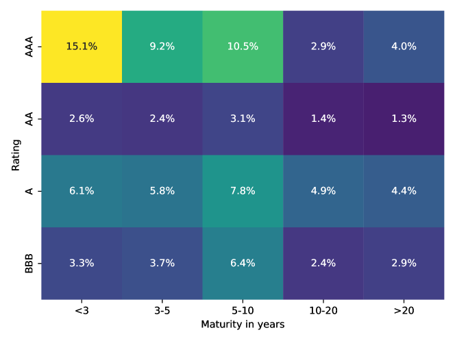
Figure 1: The nominal portfolio weights.

7.2 Uncertainty sets

We create uncertainty sets using historical daily yield curves and spreads. Data for the yield curve is obtained from the US Treasury [U.Sne], and the spreads are obtained from the Federal Reserve Bank of St. Louis [Fedne], spanning the period 1997-01-02 to 2022-09-12, for a total of 5,430 observations. As our period length is 6 months, we only consider the 9 key rate durations of 6 months, as well as 1, 2, 3, 5, 7, 10, 20, and 30 years. Joining the 9 rates with the 4 ratings, our total data is represented as a $5,430\times 13$ matrix. The mean value of each column, denoted $\mu^{\mathrm{hist}}$, as well as the nominal, i.e., most recent, yields and spreads are shown in figure 2. We use simple linear interpolation to obtain the full yield curve $y\in{\mbox{\bf R}}^{60}$.

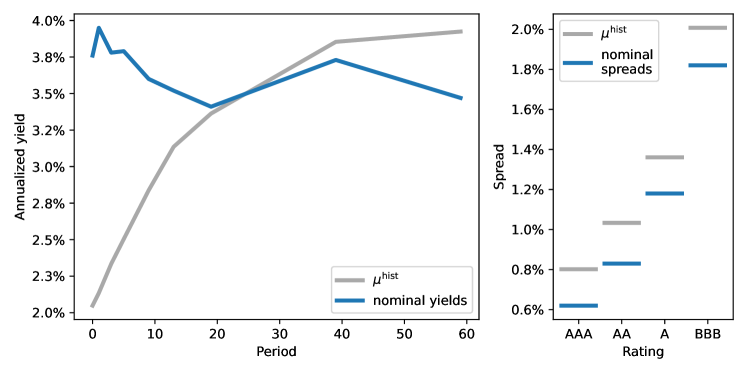
Figure 2: Historical mean values of (annualized) yield and spreads. The nominal yield and spreads, date 2022-9-12, are also shown.

We model the uncertainty set as a (degenerate) ellipsoid. We compute the empirical mean and covariance of the historical data, denoted $\mu^{\mathrm{hist}}$ and $\Sigma^{\mathrm{hist}}$, respectively. We define $Z\in{\mbox{\bf R}}^{80\times 13}$ as the matrix that maps the key rates and ratings, $({y^{\mathrm{k}}},{s^{r}})\in{\mbox{\bf R}}^{13}$ to the yields and spreads, $(y,s)\in{\mbox{\bf R}}^{80}$, i.e.,

$$(y,s)=Z(y^{\mathrm{k}},s^{r}).$$

The matrix $Z$ encodes linear interpolation between key rates; other linear mappings like spline interpolation could also be used.

Our uncertainty set is then defined in terms of key rates and ratings,

$$\mathcal{U}=\{Z(y^{\mathrm{k}},s^{r})\mid\left((y^{\mathrm{k}},s^{\mathrm{r}})-\mu^{\mathrm{hist}}\right)^{T}\left(\Sigma^{\mathrm{hist}}\right)^{-1}\left((y^{\mathrm{k}},s^{\mathrm{r}})-\mu^{\mathrm{hist}}\right)\leq F^{-1}(1-\alpha)\},$$

where $F$ is the CDF of a $\chi^{2}$ random variable with 13 degrees of freedom, and $\alpha\in(0,1)$ is a confidence level. This uncertainty set is a degenerate ellipsoid, with affine dimension $13$.

To represent a modest uncertainty set, we use confidence levels 50%. We also consider a more extreme uncertainty set, with confidence level 99%. These two uncertainty sets are meant only to illustrate our method; in practice, we would likely create uncertainty sets that change over time, and are based on more recent yield curves and spreads, as opposed to a long history of yields and spreads.

7.3 Worst case analysis

Table 2 shows worst case change in portfolio value for the 50% and 99% confidence levels, each using both the exact and linearized methods. The values are given as relative change in portfolio value, i.e., we have already converted from log returns.

$\alpha$	Worst case	Linearized
50%	-29.34%	-33.43%
99%	-39.64%	-45.95%

Table 2: Worst case change in portfolio value, for two uncertainty sets, using both the exact and linearized methods.

For $\alpha=50\%$, the exact method gives a worst case change in portfolio value of around $-29\%$, and the linearized method predicts a change in portfolio value around four percentage points lower. For $\alpha=99\%$ the approximation error of the linearized method is greater, more than six percentage points. We can see that in both cases the linearized method is conservative, i.e., predicts a change in value that is lower than the exact method.

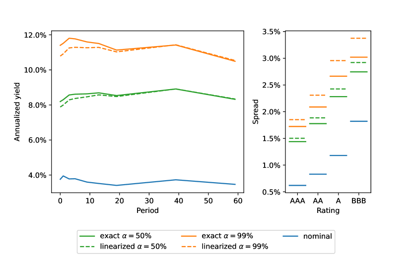
Figure 3: Worst (annualized) yield curve and spreads for the two uncertainty sets, using the exact and linearized methods.

Figure 3 shows the corresponding annualized worst case yields and spreads. For the modest uncertainty case, the linearized and exact methods produce similar results, while for the extreme case, the linearized method deviates more for shorter yields and across all spreads.

7.4 Robust portfolio construction

We now consider the case where instead of holding the nominal portfolio $h^{\mathrm{nom}}$ exactly, we try to track it, with a penalty term on the worst case change in portfolio value, as described in §4.2. Our nominal objective is the turnover distance between our holdings and the nominal portfolio, given by

$$\phi(h)=(1/2)\|h-h^{\mathrm{nom}}\|_{1}.$$

Figure 4 shows the turnover distance for both uncertainty sets and both the exact and linearized methods. For small values of $\lambda$, the nominal portfolio is held exactly. As expected, the turnover distance increases with $\lambda$, but more rapidly so for the extreme uncertainty set. We also see that the linearized method gives very similar results. For some values of $\lambda$, the resulting portfolio obtains the same turnover distance as the exact method, but for other values it is slightly worse due to the conservative linear approximation.

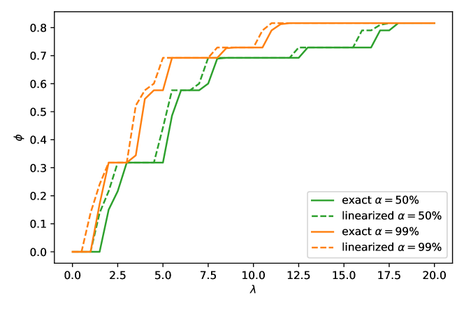
Figure 4: Turnover distance to the nominal portfolio, for two uncertainty sets, using both the exact and linearized methods.

Figure 5 shows the resulting portfolio holdings for the two uncertainty sets across varying values of $\lambda$. For $\lambda=1$, the weights are exactly the nominal weights. For $\lambda=5$, the weights have shifted to shorter maturities, reducing the worst case change in portfolio. However, this shift is more pronounced for the extreme uncertainty set, where the weights are only allocated up to the 3–5 year bucket, whereas for the modest uncertainty set the weights include bonds up to the 5–10 year bucket. A similar observation can be made for $\lambda=15$, where the optimization under the modest uncertainty set still allocates in bonds across all ratings in the bucket containing bonds with less than 3 years to maturity. In contrast, under the extreme uncertainty set the weights are only allocated to two bonds in this bucket. Specifically, the highest weight is assigned to the bond with BBB rating, and a smaller weight to the AAA bond. This is explained by the much shorter maturity of the BBB bond (see table 1), which outweighs the lower risk due to the higher rating of the AAA bond. Indeed, when manually setting the maturities of these bonds to the same value, we find that weights would be assigned to the AAA bond for large values of $\lambda$ instead.

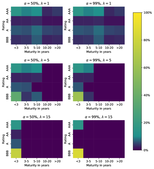
Figure 5: Portfolio holdings, for both uncertainty sets for $\lambda\in\{1,5,15\}$.

8 Conclusions

We have observed that the greatest decrease in value of a long-only bond portfolio, over a given convex set of possible yield curves and spreads, can be found exactly by solving a tractable convex optimization problem that can be expressed in just a few lines using a DSL. Current practice is to estimate the worst case decrease in value using key rate durations, which is equivalent to finding the worst case change in portfolio value using a linearized approximation of the portfolio value. We show that this estimate is always conservative. Numerical examples show that it is a good approximation of the actual worst case value for modest changes in the yield curve and spread, but less good for large uncertainty sets.

We also show that the problem of constructing a long-only bond portfolio which includes the worst case value over an uncertainty set in its objective or constraints can be tractably solved by formulating it as a convex-concave saddle point problem. Such problems can also be specified in just a few lines of a DSL.

Appendix A Worst case analysis CVXPY code

⬇

1import numpy as np

2import cvxpy as cp

3

4y = cp.Variable(T)

5s = cp.Variable(n)

6

7V = h @ p

8

9exponents = []

10for i in range(n):

11 for t_idx in range(T):

12 t = t_idx + 1 # account for 0-indexing

13 w_it = h[i] * C[i,t_idx]

14 if w_it > 0:

15 exponents.append(-t * (y[t_idx] + s[i]) + np.log(w_it))

16

17Delta = cp.log_sum_exp(cp.hstack(exponents)) - np.log(V)

18obj = cp.Minimize(Delta)

19prob = cp.Problem(obj, [A @ cp.hstack([y,s]) <= b])

20prob.solve()

Appendix B Explicit dual portfolio construction CVXPY code

⬇

1import numpy as np

2import cvxpy as cp

3

4F_1 = np.tile(np.eye(T), (n, 1))

5F_2 = np.repeat(np.eye(n), repeats=T, axis=0)

6F = np.hstack([F_1, F_2])

7

8lam = cp.Variable(len(b), nonneg=True)

9nu = cp.Variable(n * T, nonneg=True)

10

11h = cp.Variable(n, nonneg=True)

12

13B = 1

14

15term = 0

16for i in range(n):

17 for t in range(1, T):

18 nu_i_t = nu[i * T + t]

19 term -= cp.rel_entr(C[i, t] * h[i], nu_i_t / t)

20

21obj = cp.Maximize(-lam @ b + term - np.log(B))

22constraints = [

23 A.T @ lam == F.T @ nu,

24 cp.sum(nu) == 1,

25 p @ h == B,

26]

27prob = cp.Problem(obj, constraints)

28prob.solve()

Appendix C Derivation of dual form

We now derive the dual form of the worst case portfolio construction problem for the case where the uncertainty set in polyhedral. We note that the worst case $\log$ change in portfolio value for a fixed $h$, $\Delta^{\text{wc}}(h)$ is given by the optimal value of the optimization problem

$$\begin{array}[]{ll}\mbox{minimize}&\log\left(\sum_{i=1}^{n}\sum_{t=1}^{T}h_{i}c_{i,t}\exp(-t(y_{t}+s_{i}))\right)-\log(p^{T}h)\\ \mbox{subject to}&A(y,s)\preceq b.\end{array}$$

We have written this problem with $(y,s)$ explicitly, instead of with $x$, to emphasize the objective’s dependence on each component. We note that due to our budget constraint, $\log(V(y,s))=\log(p^{T}h)$.

In order to obtain a closed form dual, we introduce a new variable $z\in{\mbox{\bf R}}^{nT}$, where we think of $z_{i,t}$ as corresponding to $y_{t}+s_{i}$. This is a very general formulation which allows each bond to be associated with its own yield curve $y_{i}\in{\mbox{\bf R}}^{T}$, with $z_{i,t}$ corresponding to the $t$’th entry of the $i$’th bond’s yield curve. Since we model each bond as having its own yield curve, this formulation generalizes the earlier treatment with yields and spreads handled separately. We can recover the original structure with the linear constraints

$$z_{i,t}=y_{t}+s_{i},\qquad t=1,\ldots,T,\quad i=1,\ldots,n,$$ (16)

which are representable as $z=Fx$ for an appropriate $F\in{\mbox{\bf R}}^{nT\times(T+n)}$. As such, the problem is equivalent to

$$\begin{array}[]{ll}\mbox{minimize}&\log\left(\sum_{i=1}^{n}\sum_{t=1}^{T}h_{i}c_{i,t}\exp(-tz_{i,t})\right)-\log(p^{T}h)\\ \mbox{subject to}&Ax\preceq b,\quad z=Fx.\end{array}$$ (17)

Strong duality tells us that $\Delta^{\text{wc}}(h)$ is equal to the optimal value of the dual problem of (17) [BV04, §5.2].

Dual problem.

We derive the dual of the problem

$$\begin{array}[]{ll}\mbox{minimize}&\log\left(\sum_{i=1}^{n}\sum_{t=1}^{T}h_{i}c_{i,t}\exp(-tz_{i,t})\right)-\log(p^{T}h)\\ \mbox{subject to}&Ax\preceq b,\quad z=Fx.\end{array}$$ (18)

First, with $f$ the log-sum-exp function $f(x)=\log\left(\sum\exp x_{i}\right)$, we observe that our problem can be rewritten as

$$\begin{array}[]{ll}\mbox{minimize}&f(Cz+d)-\log(p^{T}h)\\ \mbox{subject to}&Ax\preceq b,\quad z=Fx.\end{array}$$

We define $C$ to be the diagonal matrix with $C_{i,t}=-t$, where we are using unwound vectorized indexing for $z$, and $d\in{\mbox{\bf R}}^{nT}$ to be the vector with $d_{i,t}=\log(c_{i,t}h_{i})$. Then, the Lagrangian is given by

$$L(z,x,\mu,\nu)=f(Cz+d)+\mu^{T}(Ax-c)+\nu^{T}(z-Fx)-\log(p^{T}h).$$

The Lagrange dual function is given by

$$g(\mu,\nu)=\inf_{z,x}L(z,x,\mu,\nu)=\inf_{z}\left(f(Cz+d)+\nu^{T}z\right)+\inf_{x}\left(\mu^{T}Ax-\nu^{T}Fx\right)-\mu^{T}c-\log(p^{T}h).$$

The second term is equal to $-\infty$ unless $A^{T}\mu+F^{T}\nu=0$, so this condition will implicitly restrict the domain of $g$. Now, note that with $g(z)=f(Cz+d)$, the first term can be rewritten as

$$\inf_{z}\left(f(Cz+d)+\nu^{T}z\right) = \inf_{z}\left(g(z)+\nu^{T}z\right)$$

$$= -\max_{z}\left(-\nu^{T}z-g(z)\right)$$

$$= -g^{*}(-\nu),$$

where $g^{*}(y)=\max{y}y^{T}z-g(z)$ is the conjugate of $g$. [BV04, §3.3.1].

We now use two facts from [BV04, §3.3.2]. First, in general the conjugate of the linear precomposition $\phi(z)=\rho(Cz+d)$ can be written in terms of the conjugate of $\rho$ as $\phi^{*}(y)=\rho^{*}(C^{-T}y)-d^{T}C^{-T}y$. Second, the dual of the log-sum-exp function $f$ is

$$f^{*}(y)=\left\{\begin{array}[]{ll}\sum_{i}y_{i}\log(y_{i})&\text{ if }y\geq 0,\quad\mathbf{1}^{T}y=1\\ \infty&\text{ otherwise.}\end{array}\right.$$

Combining these two facts, and expanding terms, we find that

$$g(\mu,\nu)=\left\{\begin{array}[]{ll}-\log(p^{T}h)-\mu^{T}b-\sum\limits_{i=1}^{n}\sum\limits_{t=1}^{T}\zeta(c_{i,t}h_{i},\frac{\nu_{i,t}}{t})&\text{if }A^{T}\mu-F^{T}\nu=0,\ \mathbf{1}^{T}\nu=1,\ \nu\geq 0\\ -\infty&\text{otherwise,}\end{array}\right.$$

with

$$\zeta(x,t)=-t\log(x/t)=t\log(t/x)=t\log(t)-t\log(x).$$

Thus the robust bond portfolio problem can be written as

$$\begin{array}[]{ll}\mbox{minimize}&\phi(h)-\lambda\max\limits_{\mu,\nu}~{}g(\mu,\nu)\\ \mbox{subject to}&\mu\geq 0,\quad A^{T}\mu-F^{T}\nu=0,\quad\mathbf{1}^{T}\nu=1,\quad\nu\geq 0\\ &h\in\mathcal{H},\\ \end{array}$$

where we have moved the implicit constraints in the definition of $g$ to explicit constraints in the optimization problem. Note this equivalent optimization problem has new variables $\mu$ and $\nu$. By using that $-\lambda\max_{\mu,\nu}g(\mu,\nu)=\min_{\mu,\nu}-\lambda g(\mu,\nu)$ and collecting the minimization over $h$, $\mu$, and $\nu$, we obtain the form in §5.2.

References

- [BBD+17] S. Boyd, E. Busseti, S. Diamond, R. Kahn, K. Koh, P. Nystrup, and J. Speth. Multi-period trading via convex optimization. Foundations and Trends in Optimization, 3(1):1–76, 2017.
- [Blone] Bloomberg. Bloomberg fixed income indices fact sheets and publications, Nov. 16, 2022 [Online].
- [BS16] K. Bredies and H. Sun. Accelerated Douglas-Rachford methods for the solution of convex-concave saddle-point problems. arXiv preprint arXiv:1604.06282, 2016.
- [BV04] S. Boyd and L. Vandenberghe. Convex Optimization. Cambridge University Press, 2004.
- [CP05] J. Cochrane and M. Piazzesi. Bond risk premia. American Economic Review, 95(1):138–160, 2005.
- [DB16] S. Diamond and S. Boyd. CVXPY: A python-embedded modeling language for convex optimization. The Journal of Machine Learning Research, 17(1):2909–2913, 2016.
- [EGBG09] E. Elton, M. Gruber, S. Brown, and W. Goetzmann. Modern Portfolio Theory and Investment Analysis. John Wiley & Sons, 2009.
- [Fedne] Federal Reserve Bank of St. Louis. Data: [BAMLC0A1CAAA, BAMLC0A2CAA, BAMLC0A3CA, BAMLC0A4CBBB], Nov. 16, 2022 [Online].
- [FM12] F. Fabozzi and S. Mann. The Handbook of Fixed Income Securities. McGraw-Hill Education, 2012.
- [FNB20] A. Fu, B. Narasimhan, and S. Boyd. CVXR: An R package for disciplined convex optimization. Journal of Statistical Software, 94(14):1–34, 2020.
- [FPY22] D. Filipović, M. Pelger, and Y. Ye. Stripping the discount curve-a robust machine learning approach. Swiss Finance Institute Research Paper, (22-24), 2022.
- [GB14] M. Grant and S. Boyd. CVX: Matlab software for disciplined convex programming, version 2.1. 2014.
- [GBY06] M. Grant, S. Boyd, and Y. Ye. Disciplined Convex Programming, pages 155–210. Springer US, Boston, MA, 2006.
- [JN21] A. Juditsky and A. Nemirovski. On well-structured convex–concave saddle point problems and variational inequalities with monotone operators. Optimization Methods and Software, 0(0):1–36, 2021.
- [KK06] O. Korn and C. Koziol. Bond portfolio optimization: A risk-return approach. The Journal of Fixed Income, 15(4):48–60, 2006.
- [KKF14] J. Kim, W. Kim, and F. Fabozzi. Recent developments in robust portfolios with a worst-case approach. Journal of Optimization Theory and Applications, 161(1):103–121, 2014.
- [LS91] R. Litterman and J. Scheinkman. Common factors affecting bond returns. The Journal of Fixed Income, 1(1):54–61, 1991.
- [Mar52] H. Markowitz. Portfolio selection. The Journal of Finance, 7:77–91, 1952.
- [Nem04] A. Nemirovski. Prox-method with rate of convergence for variational inequalities with Lipschitz continuous monotone operators and smooth convex-concave saddle point problems. SIAM Journal on Optimization, 15(1):229–251, 2004.
- [NY78] A. Nemirovski and D. Yudin. Cesari convergence of the gradient method of approximating saddle points of convex-concave functions. In Doklady Akademii Nauk, volume 239, pages 1056–1059. Russian Academy of Sciences, 1978.
- [NY83] A. Nemirovski and D. Yudin. Problem Complexity and Method Efficiency in Optimization. Wiley-Interscience, 1983.
- [Puh08] M. Puhle. Bond Portfolio Optimization, volume 605. Springer Science & Business Media, 2008.
- [Sio58] M. Sion. On general minimax theorems. Pacific Journal of Mathematics, 8(1):171–176, 1958.
- [SLB23] P. Schiele, E. Luxenberg, and S Boyd. Disciplined saddle point programming. arXiv preprint arXiv:2301.13427, 2023.
- [TK04] R. Tütüncü and M. Koenig. Robust asset allocation. Annals of Operations Research, 132(1):157–187, 2004.
- [UMZ+14] M. Udell, K. Mohan, D. Zeng, J. Hong, S. Diamond, and S. Boyd. Convex optimization in Julia. SC14 Workshop on High Performance Technical Computing in Dynamic Languages, 2014.
- [U.Sne] U.S. Department of the Treasury. Daily treasury par yield curve rates, Nov. 16, 2022 [Online].
- [VN28] J. Von Neumann. Zur Theorie der Gesellschaftsspiele. Mathematische Annalen, 100(1):295–320, 1928.
- [VNM53] J. Von Neumann and O. Morgenstern. Theory of Games and Economic Behavior. Princeton University Press, 1953.