Emission-line properties of IllustrisTNG galaxies: from local diagnostic diagrams to high-redshift predictions for JWST

Abstract

We compute synthetic, rest-frame optical and ultraviolet (UV) emission-line properties of galaxy populations at redshifts from $z\approx 0$ to $z=8$ in a full cosmological framework. We achieve this by coupling, in post-processing, the state-of-the-art cosmological IllustrisTNG simulations with new-generation nebular-emission models, accounting for line emission from young stars, post-asymptotic-giant-branch (PAGB) stars, accreting black holes (BHs) and, for the first time, fast radiative shocks. The optical emission-line properties of simulated galaxies dominated by different ionizing sources in our models are largely consistent with those expected from classical diagnostic diagrams and reflect the observed increase in [O iii]/H$\beta$ at fixed [N ii]/H$\alpha$ and the evolution of the H$\alpha$, [O iii]$\lambda 5007$ and [O ii] $\lambda 3727$ luminosity functions from $z\approx 0$ to $z\sim 2$. At higher redshift, we find that the emission-line galaxy population is dominated by star-forming and active galaxies, with negligible fractions of shock- and PAGB-dominated galaxies. We highlight 10 UV-diagnostic diagrams able to robustly identify the dominant ionizing sources in high-redshift galaxies. We also compute the evolution of several optical- and UV-line luminosity functions from $z=4$ to $z=7$, and the number of galaxies expected to be detectable per field of view in deep, medium-resolution spectroscopic observations with the NIRSpec instrument on board the James Webb Space Telescope. We find that 2-hour-long exposures are sufficient to achieve unbiased censuses of H$\alpha$ and [O iii]$\lambda 5007$ emitters, while at least 5 hours are required for H$\beta$, and even 10 hours will detect only progressively smaller fractions of [O ii] $\lambda 3727$, O iii] $\lambda 1663$, C iii] $\lambda 1908$, C iv $\lambda 1550$, [N ii]$\lambda 6584$, Si iii] $\lambda 1888$ and He ii $\lambda 1640$ emitters, especially in the presence of dust.

1 Introduction

Optical and ultraviolet (UV) emission from interstellar gas provides important information about the ionizing sources and the properties of the interstellar medium (ISM) in galaxies. Extensive studies of this kind have been enabled for galaxies in the local Universe by large spectroscopic surveys, such as the Sloan Digital Sky Survey (SDSS, e.g., York et al., 2000; Blanton et al., 2017). For example, optical nebular-emission lines provide useful diagnostics to distinguish between ionization by young massive stars (tracing the star formation rate, hereafter SFR), an active galactic nucleus (hereafter AGN), evolved, post-asymptotic giant branch (hereafter post-AGB) stars and fast radiative shocks (e.g., Izotov & Thuan, 1999; Kobulnicky et al., 1999; Kauffmann et al., 2003; Nagao et al., 2006; Kewley & Ellison, 2008; Morisset et al., 2016). In fact, the intensity ratios of strong emission lines, such as [O ii] $\lambda 3727$, [O i]$\lambda 6300$,H$\beta$, [O iii]$\lambda 5007$, H$\alpha$, [N ii]$\lambda 6584$ and [S ii]$\lambda 6724$, exhibit well-defined correlations sensitive to the nature of ionizing radiation. Widely used line-ratio diagnostic diagrams are those defined by [O iii]$\lambda 5007$/H$\beta$, [N ii]$\lambda 6584$/H$\alpha$, [S ii]$\lambda 6724$/H$\alpha$ and [O i]$\lambda 6300$/H$\alpha$ (hereafter simply [O iii]/H$\beta$, [N ii]/H$\alpha$, [S ii]/H$\alpha$ and [O i]/H$\alpha$), originally proposed by Baldwin et al. (1981, hereafter BPT) and Veilleux & Osterbrock (1987). These diagrams have proven efficient to distinguish active from inactive star-forming galaxies in large samples of local galaxies (e.g. Kewley et al., 2001; Kauffmann et al., 2003). Instead, identifying unambiguously galaxies for which the ISM is primarily ionized by post-AGB stellar populations or fast radiative shocks appears more difficult. In the former case, recent studies suggest that diagnostic diagrams involving the H$\alpha$ equivalent width (EW), such as EW(H$\alpha$) versus [N ii]/H$\alpha$  (hereafter the WHAN diagram, Cid Fernandes et al., 2010; Cid Fernandes et al., 2011), appear more promising. In the latter case, Baldwin et al. (1981); Kewley et al. (2019) proposed a diagnostic diagram defined by [O iii]$\lambda 5007$/[O ii] $\lambda 3727$ (hereafter simply [O iii]/[O ii]) versus [O i]/H$\alpha$.

Over the past two decades, rest-frame optical spectra have become available for increasingly large samples of more distant galaxies, at redshifts $z\sim 0.5$–3, through near-infrared (NIR) spectroscopy (e.g., Pettini & Pagel, 2004; Hainline et al., 2009; Steidel et al., 2014; Shapley et al., 2015), in particular with the NIR multi-object spectrographs MOSFIRE (McLean et al., 2010) and FMOS (Kimura, 2010). Interestingly, these observations indicate uniformly that star-forming galaxies at $z>1$ have systematically larger [O iii]/H$\beta$ ratio at fixed [N ii]/H$\alpha$ ratio than their local SDSS counterparts (see, e.g., Shapley et al., 2005; Lehnert et al., 2009; Yabe et al., 2012; Steidel et al., 2014; Shapley et al., 2015; Strom et al., 2017). The physical origin of this observation is still being debated, and several explanations have been proposed, such as higher ionization parameter, enhanced N/O abundances, harder ionizing-radiation field (e.g. due to binary star models) or weak, unresolved AGN emission in high-redshift galaxies compared to low-redshift ones (for a detailed discussion, see Hirschmann et al., 2017, and references therein).

The above spectroscopic surveys, together with deep narrow-band surveys over wide sky areas (e.g. HiZELS, Geach et al., 2008), have also allowed studies of the statistics of rest-frame optical emission-line galaxies, quantified through luminosity functions of the H$\alpha$, [O iii]$\lambda 5007$+H$\beta$ and [O ii] $\lambda 3727$ emission lines at redshifts $z\sim 0$–3 (e.g., Tresse et al., 2002; Fujita et al., 2003; Ly et al., 2007; Villar et al., 2008; Shim et al., 2009; Hayes et al., 2010; Sobral et al., 2012, 2013; Sobral et al., 2015; Colbert et al., 2013; Khostovan et al., 2015, 2018, 2020; Hayashi et al., 2018, and references therein). These emission lines, which are sensitive to the ionizing radiation from hot, massive O- and B-type stars, are often used as tracers of star formation on timescales of $\sim 10$ million years, providing insight into the evolution of the cosmic star-formation-rate density and the associated build-up of stellar mass in galaxies (as a complement to indicators based on the UV and far-infrared luminosities). Yet, the luminosity functions derived in the above studies can exhibit large scatter, because of uncertain corrections for dust attenuation, AGN contamination, selection biases, sample completeness, sample variance, filter profiles and various other factors.

In general, the observed line luminosity functions have been found to be well described by a Schechter (1976) functional form. In this context, the most recent studies appear to agree on a negligible evolution of the faint-end slope of line-luminosity functions with redshift and an increase by one or two orders of magnitude of the cutoff luminosity at the bright end ($L_{*}$) from $z=0$ to $z=2$–3 for H$\alpha$, [O iii]$\lambda 5007$+H$\beta$ and [O ii] $\lambda 3727$, reflecting the similar increase in cosmic SFR density (e.g., Sobral et al., 2015; Khostovan et al., 2015).

At redshift $z>3$, emission-line observations are generally still limited, except for a few pioneering studies (see Robertson, 2021, for a review). This situation is being revolutionized by the recently launched James Webb Space Telescope (JWST), on board of which the sensitive NIRSpec instrument (Jakobsen et al., 2022; Ferruit et al., 2022) is already detecting rest-frame optical emission lines in $z>3$ galaxies (Curti et al., 2023; Katz et al., 2022). Large such samples will be built up over the first year of operations by multiple teams, with rest-frame UV emission lines being observable out to extremely high redshifts. UV lines are particularly prominent in metal-poor, actively star-forming dwarf galaxies in the nearby Universe and have been detected in small samples of high-redshift galaxies with NIR spectrographs (e.g., Pettini & Pagel, 2004; Hainline et al., 2009; Erb et al., 2010; Stark et al., 2014; Vanzella, 2017; Senchyna et al., 2017; Talia, 2017). In addition to JWST, large surveys of high-redshift emission-line galaxies are (expected to be) observed with other current and future observational facilities, such as the Dark Energy Spectroscopic Instrument (DESI), Euclid, and the Nancy Grace Roman Space Telescope.

Despite this observational progress, interpreting observations of rest-frame optical and UV emission lines of high-redshift galaxies remains challenging, as illustrated by the persisting debate about the nature of the ionizing radiation in galaxies at $z\sim 3$ (see above). Also, at the very low metallicities expected in the youngest galaxies at high redshifts (e.g., Maiolino et al., 2008), the spectral signatures of AGN-dominated and star-formation (SF)-dominated galaxies overlap in standard optical (BPT) diagnostic diagrams (Groves et al., 2006; Feltre et al., 2016; Hirschmann et al., 2019). This led Feltre et al. (2016, see also ) to explore the location of a wide range of photoionization models of SF- and AGN-dominated galaxies in alternative, UV emission-line dianostic diagrams. While highly instructive, these pioneering studies also present some limitations: (i) the exploration of purely SF-dominated and AGN-dominated models did not account for mixed contributions by these ionizing sources, nor for contributions by post-AGB stars nor radiative shocks; (ii) the results may be biased by the inclusion of parameter combinations not found in nature; (iii) the conclusions drawn about line-ratio diagnostic diagrams do not incorporate potential effects linked to the evolution of galaxy properties with cosmic time; and (iv) these studies, based on grids of photoionization models, are not designed to explore the evolution of emission-line properties of galaxy populations (such as luminosity functions) with redshift.

A way to gain insight into the connection between emission-line properties and ionizing sources for the evolving galaxy population is to model galaxy nebular emission in a full cosmological framework. Fully self-consistent models of this kind are currently limited, mainly because of insufficient resolution of the ISM and the neglect of radiation-gas coupling in cosmological simulations. As an alternative, some studies proposed the post-processing of cosmological hydrodynamic simulations and semi-analytic models with photoionization models to compute nebular emission of galaxies in a cosmological context, albeit with the drawbacks of either following emission lines produced by only young star clusters (Kewley et al., 2013; Orsi et al., 2014; Shimizu et al., 2016; Wilkins et al., 2020; Pellegrini et al., 2020; Shen et al., 2020; Garg et al., 2022; Baugh et al., 2022), or being limited to a relatively small sample of massive galaxies (Hirschmann et al., 2017; Hirschmann et al., 2019). In the latter two studies, we included nebular emission from young star clusters, AGN and post-AGB stellar populations, but not the contribution from fast radiative shocks.

In this paper, we appeal to the same methodology as in our previous work (Hirschmann et al., 2017; Hirschmann et al., 2019) to model in a self-consistent way the emission-line properties of galaxy populations, but with two main improvements: we consider the evolution over cosmic time of a much larger sample of galaxies from the IllustrisTNG simulation, covering a full range of masses; and we incorporate the contribution to nebular emission from fast radiative shocks, in addition to the emission from young star clusters, AGN, and post-AGB stellar populations. We achieve this by coupling photoionization models for young stars (Gutkin et al., 2016), AGN (Feltre et al., 2016), post-AGB stars (Hirschmann et al., 2017) and fast, radiative shocks (Alarie & Morisset, 2019) with the IllustrisTNG cosmological hydrodynamic simulations. Our methodology, which by design captures SF-dominated, composite, AGN-dominated, post-AGB-dominated and shock-dominated galaxy populations in a full cosmological framework, offers a unique way to address several important questions:

• Are the predicted emission-line properties of IllustrisTNG galaxy populations statistically consistent with the observed, optical emission-line properties of galaxies out to $z\sim 3$, as was previously shown for only a small sample of massive galaxies (Hirschmann et al., 2017)?

• Which optical and UV diagnostic diagrams can help robustly distinguish between the main ionizing source(s) in metal-poor galaxy populations at redshifts $z>3$, and how do these diagnostics compare with the UV-based criteria derived from the limited sample of Hirschmann et al. (2019)?

• What is the expected evolution of optical and UV line-luminosity functions of galaxies at redshifts $z>3$, and how many galaxies of a given type can we expect to be detected by planned JWST/NIRSpec surveys?

Answers to these questions will allow a robust interpretation of the high-quality spectra of very distant galaxies that will be collected in the near future with JWST, providing valuable insight into, for example, the census of emission-line galaxy populations out to $z\sim 8$, and the relative contributions by star formation and nuclear activity to reionization.

The paper is structured as follows. We start by describing the theoretical framework of our study in Section 2, including the IllustrisTNG simulation set, the photoionization models and the coupling methodology between simulations and emission-line models. Section 3 presents our main findings about tracing the nature of ionizing sources in galaxy populations over cosmic time, via classical optical and novel UV diagnostic diagrams. In Section 4, we explore: (i) which UV line luminosities reliably trace the SFR in high-redshift galaxies; (ii) the cosmic evolution of optical and UV emission-line luminosity functions; and (iii) number counts of galaxy populations of different types expected to be detected with JWST/NIRSpec at high redshift. We address possible caveats of our approach and put our results into the context of previous theoretical studies in Section 5. Section 6 summarizes our main results.

2 Theoretical framework

In this paper, we model the optical and UV emission-line properties of galaxy populations in a wide redshift range using the IllustrisTNG300, IllustrisTNG100 and IllustrisTNG50 simulation suite (hereafter TNG300, TNG100 and TNG50; Pillepich et al., 2018a; Springel et al., 2018; Nelson et al., 2018; Naiman et al., 2018; Marinacci et al., 2018; Nelson et al., 2019; Pillepich et al., 2019). In the following paragraphs, we briefly summarise the simulation details (Section 2.1), the emission-line models (Section 2.2, Gutkin et al., 2016; Feltre et al., 2016; Hirschmann et al., 2017) and the coupling methodology (Section 2.3, Hirschmann et al., 2017; Hirschmann et al., 2019), referring the reader to the original studies for more details. Our novel incorporation of emission-line models of fast radiative shocks (from Alarie & Morisset, 2019), and their coupling with shocked regions identified in simulated IllustrisTNG galaxies, are described in Sections 2.2.2 and 2.3.2, respectively.

2.1 The IllustrisTNG simulation suite

IllustrisTNG is a suite of publicly available, large volume, cosmological, gravo-magnetohydrodynamical simulations, run with the moving-mesh code Arepo (Springel, 2010), and composed of three simulations with different volumes and resolutions: TNG300, TNG100 and TNG50. Each IllustrisTNG run self-consistently solves the coupled evolution of dark matter, gas, luminous stars, and supermassive black holes from a starting redshift of $z=127$ to $z=0$, assuming the currently favoured Planck cosmology ($\sigma_{8}=0.8159$, $\Omega_{\mathrm{m}}=0.3089$, $\Omega_{\Lambda}=0.6911$ and $h=0.6774$; see e.g., Planck Collaboration et al., 2016).

In brief, TNG300, TNG100 and TNG50 comprise volumes of 302.6³, 106.5³ and 51.7³ cMpc³, respectively, populated by particles with masses $m_{\mathrm{dm}}=5.9\times 10^{7}\hbox{M${}_{\odot}$}$, $7.5\times 10^{6}\hbox{M${}_{\odot}$}$ and $4.5\times 10^{5}\hbox{M${}_{\odot}$}$ for dark matter (DM), and $m_{\mathrm{bar}}=1.1\times 10^{7}\hbox{M${}_{\odot}$}$, $1.4\times 10^{6}\hbox{M${}_{\odot}$}$, and $8\times 10^{4}\hbox{M${}_{\odot}$}$ for baryons. The gravitational softening length for DM particles at $z=0$ is $1.48\ \mathrm{kpc}$, $0.74\ \mathrm{kpc}$ and $0.29\ \mathrm{kpc}$ for TNG300, TNG100 and TNG50, respectively.

All IllustrisTNG simulations include a model for galaxy formation physics (Weinberger et al., 2017; Pillepich et al., 2018b), which has been tuned to match observational constraints on the galaxy stellar-mass function and stellar-to-halo mass relation, the total gas-mass content within the virial radius of massive galaxy groups, the stellar-mass/stellar-size relation and the relation between black-hole (BH) mass and galaxy mass at $z=0$. Specifically, the simulations follow (i) primordial and metal-line radiative cooling in the presence of an ionizing background radiation field; (ii) a pressurised ISM via an effective equation-of-state model; (iii) stochastic star formation; (iv) evolution of stellar populations and the associated chemical enrichment (tracing individual elements) by supernovæ (SN) Ia/II, AGB stars and neutron-star (NS)-NS mergers; (v) stellar feedback via an kinetic wind scheme; (vi) BH seeding, growth and feedback (two-mode model for high-accretion and low-accretion phases); (vii) amplification of a small, primordial-seed magnetic field and dynamical impact under the assumption of ideal MHD. The IllustrisTNG simulations have been shown in various studies to provide a fairly realistic representation of the properties of galaxies evolving across cosmic time (e.g., Torrey et al., 2019).

In an IllustrisTNG simulation, the properties of galaxies, galaxy groups, subhaloes and haloes (identified using the FoF and Subfind substructure-identification algorithms, see Davis et al., 1985 and Springel et al., 2001, respectively), are computed ‘on the fly’ and saved for each snapshot. In the following, we always consider both central and satellite Subfind haloes and their galaxies. In addition, an on-the-fly cosmic shock finder coupled to the code (Schaal & Springel, 2015) uses a ray-tracing method to identify shock surfaces and measure their properties.

Schaal et al. (2016) describe the functioning and performances of this algorithm on Illustris-simulation data. In a first step, cells in shock-candidate regions are flagged according to certain criteria (e.g., negative velocity divergence; temperature and density gradients pointing in a same direction). Secondly, the shock surface is defined by the ensemble of cells exhibiting the maximum compression along the shock normal. Thirdly, the Mach number is estimated from the Ranking-Hugoniot temperature jump condition, and a shock is defined only if the Mach-number jump exceeds 1.3. We note that, by default, shock finding is disabled for star-forming cells, which are those lying close to the effective equation of state of the ISM in density-temperature ($\rho$-$T$) phase space. That is, shocks are not followed when either the pre-shock cell, the post-shock cell, or the cell in the shock fulfil $\rho>\rho_{\mathrm{sfr}}$ and $T<2\times 10^{4}(\rho/\rho_{\mathrm{sfr}})\,$K, where $\rho_{\mathrm{sfr}}$ is the density threshold for star formation. By definition, therefore, the IllustrisTNG simulations are not capturing shocks in the cold/warm/star-forming ISM. This also implies that shocks from supernovae explosions, which primarily occur in star-forming regions, are not captured. For more details on the shock-finder algorithm, we refer the reader to Schaal & Springel (2015) and Schaal et al. (2016).

2.2 Emission-line models

We use the same methodology as in Hirschmann et al. (2017); Hirschmann et al. (2019) to compute nebular-line emission of galaxies from the post-processing of the three tiers of IllustrisTNG simulations. At $z=0$, TNG50 has $\sim 8,800$ galaxies with stellar masses greater than $10^{8}\hbox{M${}_{\odot}$}$, TNG100 $\sim 18,000$ galaxies with stellar masses greater than $3\times 10^{9}\hbox{M${}_{\odot}$}$ and TNG300 $\sim 47,000$ galaxies with stellar masses greater than $10^{10}\hbox{M${}_{\odot}$}$. For all these galaxies and their progenitors at $z>0$, nebular emission from young star clusters (Gutkin et al., 2016), narrow-line regions (NLR) of AGN (Feltre et al., 2016) and post-AGB stars (Hirschmann et al., 2017) is computed using version c13.03 of the photoionization code Cloudy (Ferland et al., 2013), while the emission from fast radiative shocks (Alarie & Morisset, 2019) is computed using Mappings V (Sutherland & Dopita, 2017). All photoionization calculations considered in this work were performed adopting a common set of element abundances down to metallicities of a few per cent of Solar (from Gutkin et al., 2016).

2.2.1 Emission-line models of young star clusters, AGN and post-AGB stellar populations

To model nebular emission from H ii regions around young stars, AGN narrow-line regions and post-AGB stellar populations, we adopt the same photoionization models as described in section 2.2.1 of Hirschmann et al. (2019, to which we refer for details). In brief, the emission from young star clusters is described with an updated version of the Gutkin et al. (2016) photoionization calculations combining the latest version of the Bruzual & Charlot (2003) stellar population synthesis model with Cloudy, for 10 Myr-old stellar populations with constant SFR and a standard Chabrier (2003) initial mass function (IMF) truncated at 0.1 and 300 M_⊙. The emission from AGN narrow-line regions is described with an updated version of the Feltre et al. (2016) photoionization models. Finally, we adopt the ‘PAGB’ models of Hirschmann et al. (2017) to describe the emission from interstellar gas photoionized by evolved stellar populations of various ages.

The H ii-region, AGN-NLR and PAGB models are available for full ranges of interstellar metallicity, ionization parameter, dust-to-metal mass ratio, ionized-gas density, and C/O abundance ratio [except for the PAGB models with fixed (C/O)_⊙=0.44], as listed in table 1 of Hirschmann et al. (2017).

2.2.2 Emission-line models of fast radiative shocks

To describe the contribution by shock-ionized gas to nebular emission in IllustrisTNG galaxies, we appeal to the 3MdBs database3 of fully-radiative shock models computed by Alarie & Morisset (2019) using Mappings V. The models, computed in plane-parallel geometry, are available over a similarly wide range of interstellar metallicities ($Z_{\mathrm{shock}}$) to those adopted in the H ii-region, AGN-NLR and PAGB photoionization models described in the previous section [albeit with only two values of the C/O ratio: (C/O)${}_{\mathrm{shock}}=0.25\times$(C/O)_⊙ and (C/O)_⊙]. Metal depletion onto dust grains is not included in this case, as in fast shocks, dust can be efficiently destroyed by grain-grain collisions, through both shattering and spallation, and by thermal sputtering (Allen et al., 2008).

The other main adjustable parameters defining the shock-model grid are the shock velocity ($100\leq v_{\mathrm{shock}}\leq 1000\,$km s^-1), pre-shock density ($1\leq n_{\mathrm{H,shock}}\leq 10^{4}\,$cm^-2) and magnetic-field strength ($10^{-4}\leq B_{\mathrm{shock}}\leq 10\,\mu$G). We focus here on the predictions of models including nebular emission from both shocked and shock-precursor (i.e., pre-shock) gas photoionized by the shock (see Alarie & Morisset, 2019 for more details).

2.3 Coupling nebular-emission models with IllustrisTNG simulations

We combine the IllustrisTNG simulations of galaxy populations described in Section 2.1 with the photoionization models of Section 2.2 by associating, at each time step, each simulated galaxy single H ii-region, AGN-NLR, PAGB and radiative-shock models, which, when combined, constitute the total nebular emission of the galaxy. We achieve this using the procedure described in Hirschmann et al. (2017); Hirschmann et al. (2019), by self-consistently matching the model parameters available from the simulations with those of the emission-line models, a novelty here being the incorporation of the radiative-shock models (see below). The ISM and stellar parameters of simulated galaxies are evaluated by considering all ‘bound’ gas cells and star particles (as identified by the Subfind algorithm; Section 2.1) for the coupling with the H ii-region and PAGB models, and within 1 kpc around the BH for the coupling with the AGN-NLR models. We note that while the coupling methodology described in the next paragraphs pertains to galaxy-wide nebular emission (as in Hirschmann et al., 2017; Hirschmann et al., 2019), the versatile nature of our approach allows its application to spatially-resolved studies of galaxies (Hirschmann et al., in prep.).

A few photoionization-model parameters cannot be defined from the simulation, such as the slope of the AGN ionizing spectrum ($\alpha$), the hydrogen gas density in individual ionized regions ($n_{\mathrm{H}}$), the dust-to-metal mass ratio ($\xi_{\rm d}$) and the pre-shock density ($n_{\mathrm{H,shock}}$), since individual ionised regions are unresolved and dust formation is not followed. For simplicity, we fix the slope of the AGN ionizing spectrum to $\alpha=-1.7$ and adopt standard hydrogen densities $n_{\mathrm{H},\star}=10^{2}\,$cm^-3 in the H ii-region models, $n_{\mathrm{H},\bullet}=10^{3}\,$cm^-3 in the AGN-NLR models, and $n_{\mathrm{H},\diamond}=10\,$cm^-3 in the PAGB models. We mitigate the impact of the dust-to-metal mass ratio on the predicted nebular emission of the H ii-region, AGN and PAGB models by sampling two values, $\xi_{\rm d}=0.3$ and 0.5, around the Solar-neighbourhood value of $\xi_{\rm d,\odot}=0.36$ (Gutkin et al., 2016). Hirschmann et al. (2017); Hirschmann et al. (2019) discuss in detail the influence of the above parameters on predicted optical and UV emission-line fluxes. For the pre-shock density, which has a comparably weak influence on most emission lines of interest to us, we adopt for simplicity $n_{\mathrm{H,shock}}$ = 1 cm^-3, the lowest value available in the shock models, closest to the typical galaxy-wide densities sampled by the simulations.

In the next paragraphs, we provide slightly more details on the coupling of the IllustrisTNG simulations with H ii-region, AGN-NLR and PAGB photoionization models (Section 2.3.1) and radiative-shock models (Section 2.3.2).

2.3.1 Coupling simulated galaxies with H ii-region, AGN-NLR and PAGB photoionization models

At each simulation time step, we associate each simulated galaxy with the H ii-region model of closest metallicity, C/O ratio and ionization parameter. The ionization parameter of gas ionized by young star clusters in a simulated galaxy, $U_{\mathrm{sim},\star}$, depends on the simulated SFR (via the rate of ionizing photons) and global average gas density (via the filling factor $\epsilon=\rho_{\mathrm{gas,glob}}/n_{\mathrm{H},\star}$; see equations 1–2 of Hirschmann et al., 2017). As a further fine-tuning, in the present study, we calibrate the filling factor in such a way that present-day galaxies in the simulation follow the local relation between ionization parameter and interstellar metallicity, $\log U\approx-0.8\log(Z_{\mathrm{ISM}}/\hbox{Z${}_{\odot}$})-3.58$ (see figure 2 of Carton et al., 2017). At higher redshift, we take the evolution of the filling factor to follow that of the global average gas density.

The procedure to associate each simulated galaxy with an AGN-NLR and a PAGB photoionization models is identical to that described in Hirschmann et al. (2019). At each time step, we select the AGN-NLR model of metallicity, C/O ratio and ionization parameter closest to the average values computed in a co-moving sphere of 1-kpc radius around the central BH (roughly appropriate to probe the NLR for AGN with luminosities in the range found in our simulations). The PAGB model is selected to be that with age and metallicity closest to the average ones of stars older than 3 Gyr in the simulated galaxy, and with same warm-gas properties as the H ii-region model (since the simulation does not resolve gas in star-forming clouds versus the diffuse ISM).

2.3.2 Coupling simulated galaxies with radiative-shock models

To compute the contribution from radiative shocks to nebular-line emission in a simulated galaxy at a given time step, we consider all cells flagged by the shock-finder algorithm (Section 2.1) and compute their mean magnetic-field strength ($B_{\mathrm{shock,sim}}$), metallicity ($Z_{\mathrm{shock,sim}}$), C/O abundance ratio [(C/O)_shock,sim] and velocity ($v_{\mathrm{shock,sim}}$). The individual shock-cell velocities are estimated from the Mach numbers ($M$, available for each shock cell) as $v_{\mathrm{shock,sim}}=M\times v_{\mathrm{sound}}$, where $v_{\mathrm{sound}}$ is the sound speed for an ideal gas at the temperature of the cell. Then, we associate the galaxy with the radiative-shock model of closest magnetic-field strength ($B_{\mathrm{shock}}$), metallicity ($Z_{\mathrm{shock}}$), C/O abundance ratio [(C/O)_shock] and velocity ($v_{\mathrm{shock}}$).

2.4 Total emission-line luminosities, line ratios and equivalent widths of IllustrisTNG galaxies

The procedure described in the previous paragraphs allows us to compute the contributions of young stars, an AGN, post-AGB stars and fast radiative shocks to the luminosities of various emission lines (such as $L_{\mathrm{H}\alpha}$, $L_{\mathrm{H}\beta}$, $L_{\mathrm{[OIII]}}$, etc.) in a simulated galaxy. The total emission-line luminosities of the galaxy can then be calculated by summing these four contributions. For line luminosity ratios, we adopt for simplicity the notation $L_{\mathrm{[OIII]}}/L_{\mathrm{H}\beta}=\hbox{[O\,{\sc iii}]/H$\beta$}$. In this study, we focus on exploring line ratios built from six optical lines, H$\beta$, [O iii]$\lambda 5007$, [O i]$\lambda 6300$, H$\alpha$, [N ii]$\lambda 6584$ and [S ii]$\lambda 6724$  and nine UV lines, N v $\lambda 1240$ (multiplet), C iv $\lambda\lambda 1548,1551$ (hereafter simply C iv $\lambda 1550$), He ii $\lambda 1640$, O iii]$\lambda\lambda 1661,1666$ (hereafter simply O iii] $\lambda 1663$), N iii] $\lambda 1750$ (multiplet), [Si iii]$\lambda 1883$+Si iii]$\lambda 1892$ (hereafter simply Si iii] $\lambda 1888$), [C iii]$\lambda 1907$+C iii]$\lambda 1909$ (hereafter simply C iii] $\lambda 1908$), C ii] $\lambda 2326$ and [O ii]$\lambda\lambda 3726,3729$ (hereafter simply [O ii] $\lambda 3727$).

We note that, throughout this paper (except in Section 4.3), we do not consider attenuation by dust outside H ii regions and compare our predictions with observed emission-line ratios corrected for this effect By design, the above optical-line ratios are anyway rather insensitive to dust, as they are defined by lines close in wavelength (for reference, the corrections are less than $\sim 0.015$ dex for a $V$-band attenuation of $A_{V}\sim 0.5$ mag).

In addition to line luminosities and line ratios, we also compute the total equivalent widths of some nebular emission lines. We obtain the EW of an emission line by dividing the total line luminosity by the total continuum flux $C$ at the line wavelength, e.g., EW(C iii] $\lambda 1908$) $=L_{\rm CIII]}/C_{\rm CIII]}$ (expressed in Å). The total continuum $C$ is the sum of the contributions by the stellar (SF and PAGB) and AGN components. For the stellar components, we account for both attenuated stellar radiation and nebular recombination continuum. For the AGN component, we consider only the nebular recombination continuum, and do not account for any attenuated radiation from the accreting BH. This assumption should be reasonable for type-2 AGN, where direct AGN radiation is obscured by the surrounding torus, and only emission from the narrow-line region is observed. Instead, for type-1 AGN, the EWs computed here should be interpreted as upper limits. In the remainder of this study, we will focus on exploring the EWs of one optical and five UV lines: EW(H$\alpha$), EW(C iii] $\lambda 1908$), EW(C iv $\lambda 1550$), EW(O iii] $\lambda 1663$), EW(Si iii] $\lambda 1888$) and EW(N iii] $\lambda 1750$).

3 Identification of the main ionizing source(s) in galaxy populations over cosmic time

In this section, we investigate optical and UV diagnostic diagrams to identify the main ionizing sources in full galaxy populations of the TNG50 and TNG100 simulations at $z=0-7$. We focus on galaxies containing at least $\sim 1000$ star particles, corresponding to stellar masses greater than $10^{8}\hbox{M${}_{\odot}$}$ and $3\times 10^{9}\hbox{M${}_{\odot}$}$ in the TNG50 and TNG100 simulations, respectively. Note that in this section, we do not explicitly show results for TNG300 galaxies, whose emission-line properties hardly differ from those of TNG100 galaxies.

In the simulations, we distinguish between five different galaxy types, based on the predicted ratio of BH accretion rate (BHAR) to star formation rate (SFR) and the H$\beta$-line luminosity. Specifically, SF-dominated, composite, AGN-dominated, PAGB-dominated and shock-dominated galaxies are defined as follows (see also Hirschmann et al., 2017; Hirschmann et al., 2019):

• SF-dominated galaxies: BHAR/SFR $<10^{-4}$ and H$\beta_{\rm SF+AGN}>$ H$\beta_{\rm PAGB}$ + H$\beta_{\rm shock}$;

• Composite galaxies: $10^{-4}<$ BHAR/SFR $<10^{-2}$ and H$\beta_{\rm SF+AGN}>$ H$\beta_{\rm PAGB}$ + H$\beta_{\rm shock}$;

• AGN-dominated galaxies: BHAR/SFR $>10^{-2}$ and H$\beta_{\rm SF+AGN}>$ H$\beta_{\rm PAGB}$ + H$\beta_{\rm shock}$;

• PAGB-dominated galaxies: H$\beta_{\rm SF+AGN}$ + H$\beta_{\rm shock}<$ H$\beta_{\rm PAGB}$;

• Shock-dominated galaxies: H$\beta_{\rm SF+AGN}$ + H$\beta_{\rm PAGB}<$ H$\beta_{\rm shock}$.

In Section 3.1 below, we start by comparing the predicted locations of these different galaxy types at $z=0$ in the classical BPT and Mass-Excitation (MEx, Juneau et al., 2011) diagnostic diagrams with those of SDSS galaxies. We also propose alternative diagnostics to reliably identify shock-dominated and PAGB-dominated galaxies. In Section 3.2, we examine how the star formation rates and cold-gas fractions of simulated galaxies compare with those of SDSS galaxies. Then, we move on to the redshift range $z=0.5-7$ and explore, in Section 3.3, to what extent classical BPT diagrams still allow accurate separation of SF-dominated, composite and AGN galaxy populations, and whether our simulation predictions can statistically reproduce the observed evolution of [O iii]/H$\beta$ at fixed [N ii]/H$\alpha$. In Section 3.4, we investigate changes in the relative fractions of galaxies of different types with cosmic time. Finally, in Section 3.5, we confront our simulations of galaxy populations with the UV diagnostic diagrams proposed by Hirschmann et al. (2019, based on a set of only 20 zoom-in simulations of massive galaxies) to assess the robustness of these diagrams to identify different galaxy types during the epoch or reionization, as a guidance for interpreting planned spectroscopic, high-redshift galaxy surveys with, e.g., JWST/NIRSpec.

3.1 Optical diagnostic diagrams at $z=0$

Fig. 1 shows the predicted distributions of emission-line ratios of SF-dominated (left column, blue 2D histogram), composite (second column, red 2D histogram), AGN-dominated (third column, green 2D histogram), PAGB-dominated (fourth column, yellow 2D histograms) and shock-dominated (right column, lilac 2D histogram TNG100 galaxies at $z=0$ in three BPT diagnostic diagrams (top row: [O iii]/H$\beta$ versus [N ii]/H$\alpha$; middle row: [O iii]/H$\beta$ versus [S ii]/H$\alpha$; bottom row: [O iii]/H$\beta$ versus [O i]/H$\alpha$). In each panel, the predicted distribution for TNG50 galaxies is overplotted as black contours, while the grey shaded 2D histogram shows the observed distribution of SDSS galaxies. For a fair comparison between models and observations, we have imposed a typical flux-detection limit of $5\times 10^{-17}$ erg s^-1cm^-2 for simulated galaxies (motivated by table 1 of Juneau et al., 2014, as in figure 1 of Hirschmann et al., 2017).

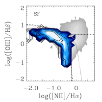
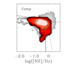
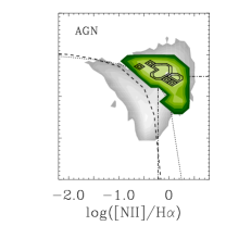
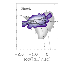
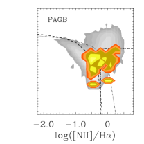
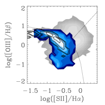
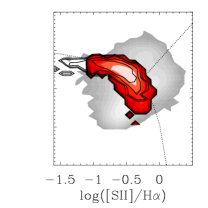
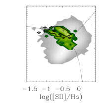
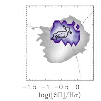
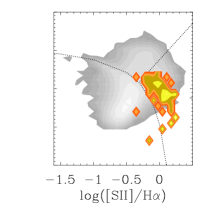
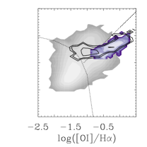
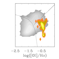
Figure 1: Location of the TNG100 galaxy population at $z=0$ in three BPT diagrams (coloured 2D histograms): [O iii]/H$\beta$ versus [N ii]/H$\alpha$ (top row), [O iii]/H$\beta$ versus [S ii]/H$\alpha$ (middle row) and [O iii]/H$\beta$ versus [O i]/H$\alpha$ (bottom row). The locations of different galaxy types (blue: SF-dominated; red: composite; green: AGN-dominated; lilac: shock-dominated; yellow: Post-AGB dominated) are shown in different columns. In each panel, the location of TNG50 galaxies is overplotted as black contours, while the grey shaded 2D histogram shows the observed distribution of SDSS galaxies. Also shown are classical empirical selection criteria. In the [O iii]/H$\beta$ vs. [N ii]/H$\alpha$ diagram, these are supposed to distinguish SF galaxies (below the dashed line) from composites (between the dashed and dotted lines), AGN (above the dotted line) and LI(N)ER (in the bottom-right quadrant defined by dot-dashed lines), according to Kewley et al. (2001, dotted line) and Kauffmann et al. (2003, dashed and dot-dashed lines). In the [O iii]/H$\beta$ vs. [S ii]/H$\alpha$ and [O iii]/H$\beta$ vs. [O i]/H$\alpha$ diagrams, SF-dominated galaxies are supposed to reside in the bottom left corner (below the curved dotted line), while AGN-dominated galaxies should occupy the top part (above the curved and straight dotted lines), and LI(N)ER the right part (right next to the curved and below the straight dotted lines), according to Kewley et al. (2001, curved dotted line) and Kewley et al. (2006, straight dotted line).

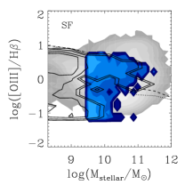
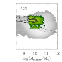
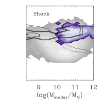
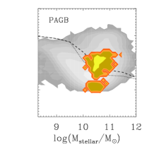
Figure 2: Location of the TNG100 and TNG50 galaxy populations at $z=0$ in the Mass-Excitation (MEx, Juneau et al., 2011) diagram. The layout and colour coding are the same as in the top row of Fig. 1. Overplotted as black dotted and dashed lines are the empirical criteria of Juneau et al. (2014) to distinguish between SF-dominated (below the dotted line), composite (between dashed and dotted lines) and AGN-dominated (above the dashed line) galaxies.

In the top-row diagrams, the black dashed and dotted lines indicate the classical empirical criteria of Kauffmann et al. (2003) and Kewley et al. (2001), respectively, to differentiate SF galaxies from composites, AGN and LI(N)ER [low-ionization (nuclear) emission] galaxies. Observationally, galaxies with line ratios below the dashed line are classified as SF-dominated, those with line ratios between the dashed and dotted lines as composites, and those with line ratios above the dotted line as AGN-dominated. In addition, galaxies with line ratios in the bottom-right quadrant defined by dot-dashed lines are classified as LI(N)ER, whose main ionizing sources are still debated (e.g., faint AGN, post-AGB stellar populations, shocks or a mix of these sources; e.g., Belfiore, 2016). The lines in the middle- and bottom-row diagrams of Fig. 1 show other criteria by Kewley et al. (2001, 2006) to separate SF-dominated (below the curved dotted line) from AGN-dominated (above both dotted lines) and LI(N)ER (in the bottom right area) galaxies.

As expected from the results obtained by Hirschmann et al. (2017); Hirschmann et al. (2019) for a small sample of massive, re-simulated galaxies, we find that the TNG50 and TNG100 galaxy populations at $z=0$ overlap with SDSS galaxies in all BPT diagrams in Fig. 1. Moreover, the predicted locations of SF-, AGN- and PAGB-dominated galaxy populations largely coincide with the SF, AGN and LI(N)ER areas defined by standard criteria. Composite galaxies extend over a larger area than expected from the standard criteria toward the AGN region, while shock-dominated galaxies lie preferentially at high $\log(\hbox{[O\,{\sc iii}]/H$\beta$})\ga 0$ and $\log(\hbox{[O\,{\sc i}]/H$\alpha$})\ga-1$, with [N ii]/H$\alpha$ and [S ii]/H$\alpha$ similar to those of other galaxy types.

We note that SF-dominated and composite galaxies reach lower [N ii]/H$\alpha$, [S ii]/H$\alpha$ and [O i]/H$\alpha$ ratios in the TNG50 population, which samples lower stellar masses and metallicities than the TNG100 simulation. Likewise, there are hardly any PAGB-dominated TNG50 galaxies. Such galaxies are typically more massive than $3\times 10^{10}\hbox{M${}_{\odot}$}$ and therefore significantly less numerous than in the eight-fold larger TNG100 volume.

It is interesting to note that, while PAGB dominated galaxies account for only 3 percent of all emission-line galaxies in the TNG100 simulation at $z=0$, they make up $\sim 20$ per cent of galaxies residing in the LI(N)ER area of the [O iii]/H$\beta$ vs. [N ii]/H$\alpha$ diagram. In the TNG300 simulation, which has a higher stellar mass cut and better statistics for massive galaxies, PAGB-dominated galaxies make up $\sim 40$ per cent of all LI(N)ER. Thus, the assumption often made in observational studies that LI(N)ER are typically weak AGN can potentially strongly bias statistics, such as, for example, the optical AGN luminosity function and the AGN luminosity-SFR relation.

Similarly to PAGB-dominated galaxies, shock-dominated galaxies are relatively rare, representing at most 10 per cent of all emission-line galaxies at $z=0$ in TNG100 (the fraction is lower in TNG50, because of the lower percentage of massive galaxies). Nevertheless, shocks contribute 5 to 20 per cent of the H$\beta$-line emission from 81 per cent of SF-dominated galaxies, 98 per cent of composites, 97 per cent of AGN-dominated galaxies and 51 per cent of PAGB-dominated galaxies.

In Fig. 2, we show the analogue of Fig. 1 for the MEx diagram (Juneau et al., 2011), defined by the [O iii]/H$\beta$ ratio and galaxy stellar mass $M_{\mathrm{stellar}}$. The dotted and dashed lines indicate empirical criteria from Juneau et al. (2014) to distinguish between SF-dominated (below the dotted line), composite (between dotted and dashed line) and AGN-dominated (above the dashed line) galaxies. We find that AGN-dominated galaxies in the TNG100 simulation mostly overlap with the observationally-defined AGN region. However, the [O iii]/H$\beta$ ratios of AGN-dominated galaxies with lower stellar masses sampled by TNG50 fall below the expectation. Shock-dominated galaxies lie in the same area and are therefore hardly distinguishable from AGN. Instead, SF-dominated and composite galaxies extend beyond the area identified by Juneau et al. (2014) in this diagram. In the stellar mass range $M_{\mathrm{stellar}}=3\times 10^{10}$–$10^{11}\,\hbox{M${}_{\odot}$}$, both populations can reach $\hbox{[O\,{\sc iii}]/H$\beta$}\sim 1$, i.e., an order of magnitude above expectation.

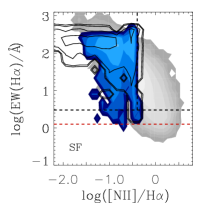
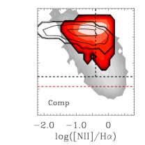
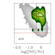
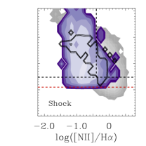
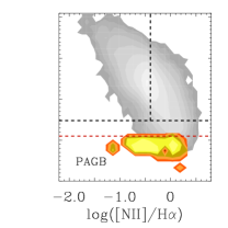
Figure 3: Location of the TNG100 and TNG50 galaxy populations at $z=0$ in the EW(H$\alpha$)-versus-[N ii]/H$\alpha$ (WHAN) diagnostic diagram (Cid Fernandes et al., 2010). The layout and colour coding are the same as in the top row of Fig. 1. Overplotted as black dashed lines in each panel are the empirical criteria of Cid Fernandes et al. (2011) to distinguish between SF-dominated (top-left quadrant), AGN-dominated (top-right quadrant), and retired, post-AGB dominated (below horizontal dashed black line) galaxies. The red dashed line shows the criterion suggested by our simulated emission-line galaxies to robustly identify post-AGB-dominated galaxies.

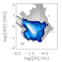
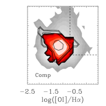
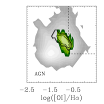
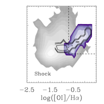
Figure 4: Location of the TNG100 and TNG50 galaxy populations at $z=0$ in the [O iii]/[O ii]-versus-[O i]/H$\alpha$ diagnostic diagram proposed by Kewley et al. (2019). The layout and colour coding are the same as in the top row of Fig. 1. In each panel, the top-right quadrant delimited by dashed black lines is the region expected to be populated only by galaxies dominated by fast radiative shocks (see figure 11 of Kewley et al., 2019).

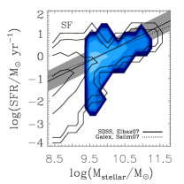
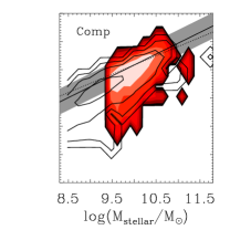
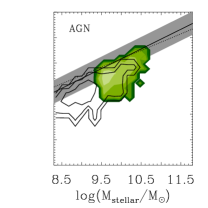
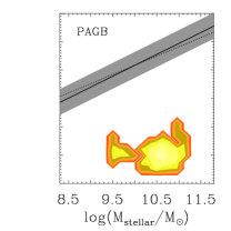
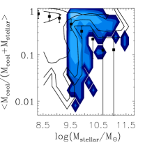
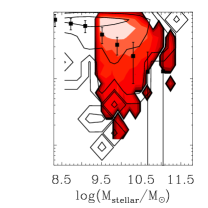
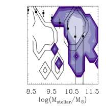
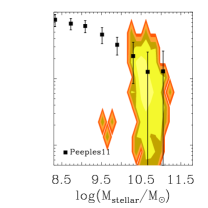
Figure 5: Location of the TNG100 and TNG50 galaxy populations at $z=0$ in the SFR-versus-stellar mass (top row) and cool-gas fraction-versus-stellar mass (bottom row) diagrams. The layout and colour coding are the same as in the top row of Fig. 1. Also shown by the black solid and dotted lines in the top diagrams are the observed main sequences of local star-forming galaxies from SDSS and GALEX data, respectively (Elbaz et al., 2007; Salim et al., 2007, the grey shaded area indicates the 1$\sigma$ scatter about the solid line). In the bottom panels, the black squares with 1$\sigma$ error bars are observed mean gas fractions from various samples of $z\sim 0$ galaxies compiled by Peeples & Shankar (2011).

The diagnostic diagrams discussed so far in Figs 1 and 2 do not allow us to uniquely identify shock-dominated and PAGB-dominated galaxies. We may appeal for this to other diagnostic diagrams, such as the EW(H$\alpha$)-versus-[N ii]/H$\alpha$ (WHAN) diagram (Stasińska et al., 2008; Cid Fernandes et al., 2010; Cid Fernandes et al., 2011; Stasińska et al., 2015), expected to help distinguish PAGB-dominated galaxies among LI(N)ER, and the [O iii]/[O ii]-versus-[O i]/H$\alpha$ diagram (Kewley et al., 2019), expected to help distinguish between shock-dominated and other types of galaxies. We show the analogues of Fig. 1 for these two additional diagnostic diagrams in Figs 3 and 4, respecively.

The black dashed lines in Fig. 3 show the empirical selection criteria of Cid Fernandes et al. (2011), which divide the WHAN diagram into three rectangles. SF-dominated galaxies are expected to reside in the top-left rectangle, AGN-dominated galaxies in the top-right one, and PAGB-dominated galaxies (referred to as ‘retired’ galaxies by Cid Fernandes et al., 2011) in the bottom one, corresponding to $\rm EW(\hbox{H$\alpha$})<3\,$Å.

Fig. 3 shows that the TNG100 and TNG50 simulated galaxies roughly overlap with SDSS galaxies in the WHAN diagram. As expected, the predicted H$\alpha$ equivalent widths of PAGB-dominated galaxies lie below those of any other considered galaxy type, with $\rm EW(\hbox{H$\alpha$})\la 1.25$ Å. This is less than half the value of 3 Å  proposed by Cid Fernandes et al. (2011), although this difference may arise in part from our definition of PAGB-dominated galaxies. Had we considered as PAGB-dominated all galaxies where PAGB stars contribute at least 40 (instead of 50) per cent of the total H$\beta$ luminosity, the upper limit (red line) in Fig. 3 would lie around $\rm EW(\hbox{H$\alpha$})\sim 3$–4 Å. Also, in our models, the predicted H$\alpha$ luminosities of PAGB-dominated galaxies rely on PAGB evolutionary tracks from Miller Bertolami (2016, incorporated in the latest version of the code), with shorter lifetimes (but higher luminosities) than in previous widely used prescriptions. Adopting older PAGB models would enhance the predicted EW(H$\alpha$) of PAGB-dominated galaxies (Section 5.1). In any case, neither changing the definition of PAGB-dominated galaxies nor using older PAGB models would introduce any confusion between PAGB-dominated and SF- or shock-dominated galaxies in Fig. 3. Only the separating EW(H$\alpha$) value would change.

In Fig. 4, the black dashed lines delimit the top-right region of the [O iii]/[O ii]-versus-[O i]/H$\alpha$ diagram expected to be populated by galaxies whose line emission is dominated by fast radiative shocks, according to Kewley et al. (2019, their figure 11). The different types of TNG50 and TNG100 galaxy populations in the different diagrams of Fig. 4 all fall on the footprint of SDSS galaxies, indicating the ability of our models to account for these observations. Furthermore, the simulated shock-dominated galaxies are the only ones to populate the top-right region noted by Kewley et al. (2019), confirming the robustness of this diagnostic diagram to separate shock-dominated galaxies from other galaxy types.

Overall, we consider the agreement between simulated and observed galaxy populations of different types at $z=0$ in the different diagnostic diagrams of Figs. 1–4 as remarkable, given that, in our approach, different galaxy types are assigned on the basis of physical parameters, such as fractional contribution to the total H$\beta$ luminosity and BHAR/SFR ratio, rather than of observables. Our results confirm previous suggestions that the [O iii]/H$\beta$-versus-[N ii]/H$\alpha$, EW(H$\alpha$)-versus-[N ii]/H$\alpha$ and [O iii]/[O ii]-versus-[O i]/H$\alpha$  diagrams, a 5D line-ratio diagnostics, provide powerful means of distinguishing between SF-, AGN-, PAGB- and shock-dominated galaxies in the nearby Universe.

3.2 SFR and cool-gas fraction

After having divided the simulated galaxy populations into different types based on their dominant ionizing sources, and explored their location in various diagnostic diagrams, we continue in this Section to study some of the predicted properties of the different galaxy types at $z=0$, such as SFR and baryonic fraction in the ‘cool-gas’ phase (i.e., gas with $T<10^{5}\,$K). We define the cool-gas fraction as $M_{\mathrm{cool}}/(M_{\mathrm{cool}}+M_{\mathrm{stellar}})$, where $M_{\mathrm{cool}}$ and $M_{\mathrm{stellar}}$ are the cool-gas and stellar masses.

In the top row of Fig. 5, we show the distributions of SFR versus $M_{\mathrm{stellar}}$ for the different types of TNG100 and TNG50 galaxy populations, using the same layout and colour coding as in Fig. 1. The observed ‘main sequence’ (MS) of local star-forming galaxies is depicted by the black solid and dotted lines for SDSS and GALEX data, respectively (Elbaz et al., 2007; Salim et al., 2007). SF-dominated and composite galaxies in our simulations largely follow this observed MS (left two panels), while AGN-dominated galaxies have SFRs typically 1–1.5 dex lower at fixed $M_{\mathrm{stellar}}$ (central panel). The shock- and PAGB-dominated galaxies (right two panels) are typically more massive, with $M_{\mathrm{stellar}}\ga 3\times 10^{10}\hbox{M${}_{\odot}$}$, and even less star-forming that the other galaxy types. Shock-dominated galaxies span a wide range of SFRs, between 1 and 10^-4 M_⊙ yr^-1, filling the so-called ‘green valley’ of the SFR-versus-stellar mass plane (e.g., Salim, 2014). PAGB-dominated galaxies are fully quiescent (retired) massive galaxies, with SFRs below $0.01\,\hbox{M${}_{\odot}$}\,$yr^-1.

The sequence of decreasing SFRs from AGN-, to shock-, to PAGB-dominated galaxies at fixed stellar mass in Fig. 5 reflects the process of SF quenching by AGN feedback in IllustrisTNG galaxies (Weinberger et al., 2017; Nelson et al., 2018; Terrazas et al., 2020): in an AGN-dominated galaxy, feedback from the heavily accreting central black hole reduces star formation. This also regulates BH growth, via a drop in gas-accretion rate. The kinetic-feedback mode associated with the low BH-accretion phase (Section 2.1) causes shocks to emerge in the ISM, heating and expelling gas from the galaxy. This further lowers the SFR and produces shock-dominated line emission. After this phase, the galaxy becomes quiescent/retired, with very low levels of on-going star formation and BH accretion, so that PAGB stars can dominate line emission.

In the bottom row of Fig. 5, we show the distributions of cool-gas fraction versus stellar mass for the different TNG100 and TNG50 galaxy populations. Also plotted for reference are observed mean gas fractions from various samples of $z\sim 0$ galaxies compiled by Peeples & Shankar (2011, black squares). Consistently with our findings above regarding star formation, we find that SF-dominated, composite, AGN-dominated, shock-dominated and PAGB-dominated galaxies represent a sequence of decreasing cool-gas fractions. We note that, at the end of the sequence, over 95 per cent of the stars in PAGB-dominated galaxies are older than 1 Gyr, with mean stellar ages greater than 6 Gyr and mean stellar metallicities between 0.6 and 1.2 times solar, i.e., typically more metal-rich than other galaxy types.

3.3 Evolution of galaxy populations in the [OIII]/H$\beta$-versus-[NII]/H$\alpha$ diagram

Based on the overall good agreement between predicted and observed distributions of different types of galaxy populations at $z=0$ (Section 3.1), we now investigate the evolution of TNG100 and TNG50 galaxy populations in the [O iii]/H$\beta$-versus-[N ii]/H$\alpha$ diagnostic diagram at higher redshift. In particular, we are interested in the extent to which the larger statistics together with different physical models offered by the IllustrisTNG simulations alter the conclusions drawn by Hirschmann et al. (2017), using a small set of 20 cosmological zoom-in simulations of massive galaxies and their progenitors, regarding the apparent rise in [O iii]/H$\beta$ at fixed [N ii]/H$\alpha$ from $z=0$ to $z=2$ in observational samples.

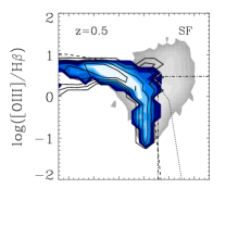
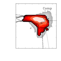
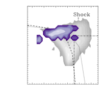
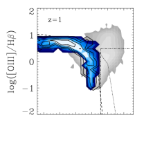
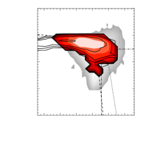
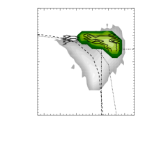
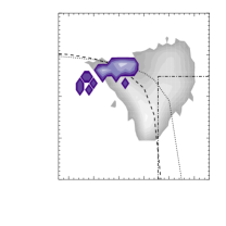
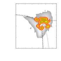
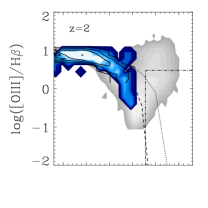
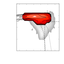
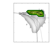
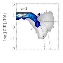
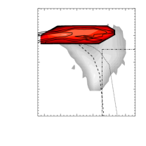
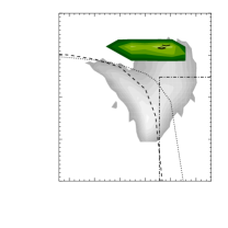
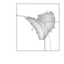
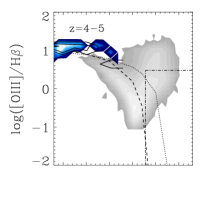
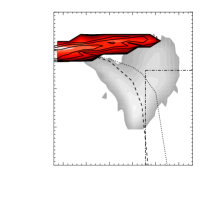
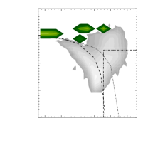
Figure 6: Redshift evolution of the location of simulated TNG100 and TNG50 galaxy populations in the [O iii]/H$\beta$-versus-[N ii]/H$\alpha$ diagnostic diagram. Rows from top to bottom show the distributions at redshifts $z=0.5$, 1, 2, 3, 4–5 and 5–7, as indicated. The layout and colour coding are the same as in the top row of Fig. 1.

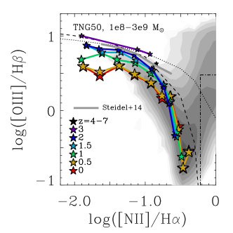
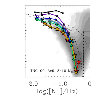
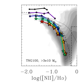
Figure 7: Average [O iii]/H$\beta$ ratio in bins of [N ii]/H$\alpha$ ratio for low-mass TNG50 galaxies ($M_{\mathrm{stellar}}=0.1$–$3\times 10^{9}\,\hbox{M${}_{\odot}$}$, left panel), intermediate-mass TNG100 galaxies ($M_{\mathrm{stellar}}=0.3$–$3\times 10^{10}\,\hbox{M${}_{\odot}$}$, middle panel) and massive TNG100 galaxies ($M_{\mathrm{stellar}}>3\times 10^{10}\,\hbox{M${}_{\odot}$}$, right panel) at different redshifts (different colours, as indicated). Also shown for reference are the same SDSS data and empirical selection criteria as in the top row of Fig. 1, along with the mean relation observed in a sample of 251 star-forming galaxies at $z\sim 2.3$ by Steidel et al. (2014, thick grey solid line).

The different rows of Fig. 6 show the distributions of TNG100 and TNG50 galaxies in the [O iii]/H$\beta$-versus-[N ii]/H$\alpha$ diagram at redshifts $z=0.5$, 1, 2, 3, 4–5 and 5–7 (from top to bottom), using the same layout and colours as for the $z=0$ distributions in the top row of Fig. 1 (except for the highest-redshift bin in the bottom row of Fig. 6, where we show the few assembled TNG100 galaxies as individual symbols). The adopted flux-detection limit cut is the same as in Fig. 1.

The lack of shock-dominated and PAGB-dominated galaxies at redshifts $z>1$ in Fig. 6 reflects the generally higher star-formation and BH-accretion rates at these early epochs. Moreover, for all the simulated galaxy types, [O iii]/H$\beta$ appears to globally increase and [N ii]/H$\alpha$ decrease from low to high redshift. This can be traced back to a drop in interstellar metallicity (the models include secondary Nitrogen production) combined with a rise in SFR and global gas density (controlling the ionization parameter) in the models, as discussed in detail in Hirschmann et al. (2017); Hirschmann et al. (2019). The global drop in [N ii]/H$\alpha$ toward higher redshifts implies that the SF-dominated, composite and AGN-dominated galaxies become less distinguishable in this classical BPT diagram (see also figure 14 of Feltre et al., 2016). This validates, on the basis of a much larger sample of simulated galaxies, the finding by Hirschmann et al. (2019) that standard optical selection criteria to identify the nature of the dominant ionizing source break down for metal-poor galaxies at $z>1$.

Motivated by a number of observational studies (e.g., Steidel et al., 2014; Shapley et al., 2015; Kashino et al., 2017; Strom et al., 2017), we focus on the redshift evolution of [O iii]/H$\beta$ for SF-dominated galaxies. Fig. 7 shows the average [O iii]/H$\beta$ ratio in [N ii]/H$\alpha$ bins for low-mass TNG50 galaxies ($M_{\mathrm{stellar}}=0.1$–$3\times 10^{9}\,\hbox{M${}_{\odot}$}$, left panel), intermediate-mass TNG100 galaxies ($M_{\mathrm{stellar}}=0.3$–$3\times 10^{10}\,\hbox{M${}_{\odot}$}$, middle panel) and massive TNG100 galaxies ($M_{\mathrm{stellar}}>3\times 10^{10}\,\hbox{M${}_{\odot}$}$, right panel) at different redshifts (different colours, as indicated). In all stellar-mass ranges, [O iii]/H$\beta$ exhibits a significant rise at a fixed [N ii]/H$\alpha$ from low to high redshifts, most pronounced with an increase of up to 1 dex for intermediate-mass galaxies (middle panel).

A remarkable result from Fig. 7 is the agreement between the predicted emission-line properties of simulated galaxies at $z\sim 2$ (blue symbols) and the observations of a sample of 251 star-forming galaxies with stellar masses in the range $M_{\mathrm{stellar}}=4\times 10^{8}$–$2.5\times 10^{11}\,\hbox{M${}_{\odot}$}$ at $z\sim 2.3$ by Steidel et al. (2014, thick grey solid line). To gain insight into the physical origin of the rise in [O iii]/H$\beta$ at high redshift, we have conducted an analysis similar to that discussed in section 4 of Hirschmann et al. (2017) by exploring separately the relative influence of different physical parameters on observables, but using now the much larger sample of simulated IllustrisTNG galaxies. Our analysis confirms our previous finding that the increase in [O iii]/H$\beta$ at a fixed galaxy stellar mass and [N ii]/H$\alpha$ from low to high redshifts is largely driven by an increase in the ionization parameter resulting from the rise in SFR and global gas density.

3.4 Galaxy-type fractions over cosmic time

In Fig. 6 above, we have seen that PAGB- and shock-dominated galaxies tend to disappear from emission-line diagrams at redshifts $z\ga 1$. Fig. 8 quantifies how the fraction of galaxies of different types evolves with redshift in the TNG100 (solid lines) and TNG50 (dashed lines) simulations (using the same colour coding as in Figs 1–6). To assess the possible impact of resolution effects on inferred galaxy type fractions, we also show the results obtained when adopting for TNG50 galaxies the same stellar-mass cut as in the TNG100 simulation, i.e., $M_{\mathrm{stellar}}>3\times 10^{9}\,\hbox{M${}_{\odot}$}$ (dot-dashed lines). For clarity, the areas encompassed by all curves referring to a given galaxy type are colour-shaded.

Fig. 8 shows that, at low redshift ($z\la 1$), the emission-line populations in the TNG100 and TNG50 simulations consist primarily of SF-dominated galaxies. Specifically, at $z=0$, the TNG100 (TNG50) population consists of about 40 (69) per cent of SF-dominated galaxies, 37 (21) per cent of composites, 10 (4) per cent of AGN-dominated galaxies, 10 (6) per cent of shock-dominated and 3 ($\ll 1$) per cent of PAGB-dominated galaxies. The different fractions found for the TNG100 and TNG50 simulations (solid and dashed lines, respectively) follow from the different stellar-mass distributions: at fixed mass cut, these fractions (solid and dot-dashed lines, respectively) are roughly consistent with one another, indicating no significant resolution effect at low redshift.

At higher redshift, the fraction of SF-dominated galaxies increases from 60 to 80 per cent over the range $1\la z\la 5$ in the TNG100 simulation, while the fraction of composites drops from 25 to 18  per cent. In the TNG50 simulation, instead, the fraction of composites increases slightly at the expenses of SF-dominated galaxies, irrespective of the stellar-mass cut. This difference relative to TNG100 may arise from resolution effects, with higher BH-accretion rates – likely due to higher gas densities in the accretion regions around the BHs – being captured by the TNG50 simulation over this redshift interval. In both simulations, the fractions of shock- and PAGB-dominated galaxies drop below 1 per cent at $z>1$, implying negligible contributions to line emission (Fig. 6). Also, the fraction of AGN-dominated galaxies falls to only 2–3 per cent from $z\sim 1$ to $z\sim 5$, because of the higher star-formation activity of high-redshift galaxies compared to their local counterparts, which can more efficiently outshine AGN emission.

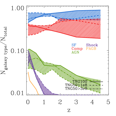
Figure 8: Fractions of galaxies of different types in the IllustrisTNG simulations plotted against redshift. The colour coding is the same as in Figs 1–6 (SF-dominated: blue; composites: red; AGN-dominated: green; shock-dominated: lilac; PAGB-dominated: yellow). Solid lines refer to TNG100 galaxies more massive than $M_{\mathrm{stellar}}=3\times 10^{9}\hbox{M${}_{\odot}$}$ and dashed and dot-dashed lines to TNG50 galaxies more massive than $M_{\mathrm{stellar}}=1\times 10^{8}$ and $3\times 10^{9}\,\hbox{M${}_{\odot}$}$, respectively. For clarity, the areas encompassed by all curves referring to a given galaxy type are colour-shaded.

3.5 UV emission-line diagnostic diagrams for metal-poor galaxies

We have seen in Section 3.3 that optical emission-line diagnostic diagrams can help reliably distinguish active from inactive galaxies out to $z\sim 1$, but start to break down for metal-poor galaxies above this redshift. We now investigate the ability of 12 UV emission-line diagnostic diagrams highlighted by Hirschmann et al. (2019, using a small set of 20 cosmological zoom-in simulations of massive galaxies and their progenitors) to help identify the dominant ionizing sources in metal-poor TNG100 and TNG50 galaxies at redshifts $z>1$. These diagrams are:

(i) EW(C iii] $\lambda 1908$) versus C iii] $\lambda 1908$/He ii $\lambda 1640$;
(ii) EW(C iv $\lambda 1550$) versus C iv $\lambda 1550$/He ii $\lambda 1640$;
(iii) EW(O iii] $\lambda 1663$) versus O iii] $\lambda 1663$/He ii $\lambda 1640$;
(iv) EW(Si iii] $\lambda 1888$) versus Si iii] $\lambda 1888$/He ii $\lambda 1640$;
(v) EW(N iii] $\lambda 1750$) versus N iii] $\lambda 1750$/He ii $\lambda 1640$;
(vi) C iii] $\lambda 1908$/He ii $\lambda 1640$ versus C iii] $\lambda 1908$/C iv $\lambda 1550$;
(vii) C iii] $\lambda 1908$/He ii $\lambda 1640$ versus N v $\lambda 1240$/He ii $\lambda 1640$;
(viii) C iii] $\lambda 1908$/He ii $\lambda 1640$ versus O iii] $\lambda 1663$/He ii $\lambda 1640$;
(ix) C iii] $\lambda 1908$/He ii $\lambda 1640$ versus Si iii] $\lambda 1888$/He ii $\lambda 1640$;
(x) C iii] $\lambda 1908$/He ii $\lambda 1640$ versus N iii] $\lambda 1750$/He ii $\lambda 1640$;
(xi) C iv $\lambda 1550$/C iii] $\lambda 1908$ versus C iii] $\lambda 1908$/C ii] $\lambda 2326$;
(xii) C iv $\lambda 1550$/C iii] $\lambda 1908$ versus [O i]$\lambda 6300$/H$\alpha$.

In Fig. 9, we show the locations in these UV diagnostic diagrams of metal-poor galaxy populations of different types from the TNG100 simulation in the redshift interval $z=1$-5 (top 12 panels), and the TNG50 simulation in the redshift interval $z=5$–7 (bottom 12 panels). The galaxies were selected to have ${\rm N2O2}<-0.8$, corresponding roughly to metallicities below $0.5\hbox{Z${}_{\odot}$}$ (Hirschmann et al., 2019). This selection makes the contribution to line emission by post-AGB stellar populations negligible, and we ignore it here (this contribution is most important in evolved, metal-rich galaxies at low redshift; see, e.g., Hirschmann et al., 2017). We note that, by analogy with Hirschmann et al. (2019), we have applied a flux-detection limit of $\rm 10^{-18}\,erg\,s^{-1}cm^{-2}$ to all emission lines when building Fig. 9. This corresponds roughly to the point-source emission-line flux sensitivity reached in $10^{4}$ s using NIRSpec on board JWST, with a signal-to-noise ratio of 10. We also applied a detection limit of 0.1 Å on emission-line EWs. This low EW limit is justified by our desire to keep our analysis as general as possible for the proposed diagnostic diagrams to be useful also for future instruments with very high sensitivity (e.g., MOSAIC and HARMONI on the Extremely Large Telescope). We have checked that the results shown in this section do not change qualitatively when applying more rigorous cuts in UV-line fluxes and EWs.

Each panel of Fig. 9 also indicates the selection criteria identified by Hirschmann et al. (2019) to discriminate between SF-dominated and composite galaxies (black dashed line), and between composite and AGN-dominated galaxies (black dotted line). Since we already validated these UV-selection criteria against observational data in Hirschmann et al. (2019), for clarity, we do not report these observations in Fig. 9.

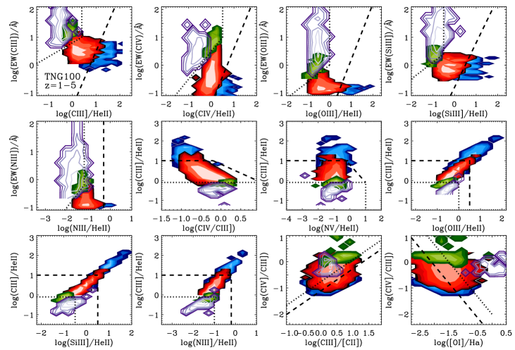
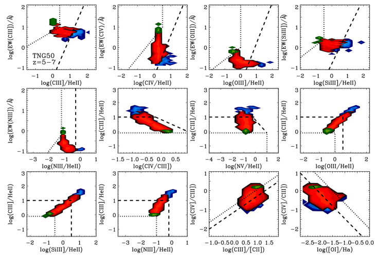
Figure 9: Location of metal-poor (${\rm N2O2}<-0.8$) galaxy populations in the TNG100 simulation at $z=1$–5 (top 12 panels) and the TNG50 simulation at $z=5$–7 (bottom 12 panels), in 12 different UV-diagnostic diagrams highlighted by Hirschmann et al. (2019, see Section 3.5 for details). A flux-detection limit of $\rm 10^{-18}\,erg\,s^{-1}cm^{-2}$ was applied to all UV emission lines. Each panel shows the 2D distributions of SF-dominated (blue), composite (red) and AGN-dominated (green) galaxies; the top 12 panels also show the distribution of shock-dominated galaxies (lilac contours; no such galaxies are predicted to be found at $z=5$–7). Overplotted in each panel are the selection criteria of Hirschmann et al. (2019) to discriminate between SF-dominated and composite galaxies (black dashed line), and between composite and AGN-dominated galaxies (black dotted line).

The first 12 panels of Fig. 9 show how shock-dominated galaxies largely fall in areas populated by AGN-dominated (and composite) galaxies in these diagrams. Thus, the UV-diagnostic diagrams shown here do not allow unique identification of galaxies, whose nebular emission is dominated by fast, radiative shocks. Given the scarcity of such galaxies in the simulations at $z>1$ (Fig. 8), we do not regard this degeneracy as problematic.

In contrast, Fig. 9 clearly demonstrates that the first 10 UV-diagnostic diagrams [labelled (i) to (x)] in the above list can robustly discriminated between SF-dominated, composite and AGN-dominated galaxies over the full redshift range $1\la z\la 7$, based on the large statistical sample of galaxies in the TNG100 and TNG50 simulations. This confirms the results obtained using a much smaller set of 20 cosmological zoom-in simulations of massive galaxies and their progenitors by Hirschmann et al. (2019). As described in that study, the reason for the good separability of different galaxy types is mainly that the ratio of any of the five considered (collisionally excited) metal lines to the He ii $\lambda 1640$ (recombination) line successively decreases from SF-dominated, to composite, to AGN-dominated galaxies. This is because of the harder ionizing radiation of accreting BHs compared to that of stellar populations, which increases the probability of producing doubly-ionized helium. We note that this is less the case for N v $\lambda 1240$/He ii $\lambda 1640$, since N v $\lambda 1240$ requires photons of even higher energy than He ii $\lambda 1640$ to be produced (77.5 versus 54.4 eV). Hence, N v $\lambda 1240$/He ii $\lambda 1640$ is not a clear indicator of the hardness of the ionizing radiation. Also the C iv $\lambda 1550$/C iii] $\lambda 1908$ ratio is sensitive to the presence of hard AGN radiation, which increases the probability of triply ionizing carbon. We note that the completeness and purity fractions (not shown) of SF-dominated, composite and AGN-dominated galaxies in the diagrams of Fig. 9 corresponding to the diagnostics (i)–(x) above all exceed 75 per cent over the full considered redshift range, further confirming the reliability of these UV-diagnostic diagrams.

To avoid having to rely on the He ii $\lambda 1640$ line, whose high strength can sometimes be challenging to model in some metal-poor star-forming galaxies (e.g., Senchyna et al., 2017; Steidel et al., 2016; Berg et al., 2018; Jaskot & Ravindranath, 2016; Wofford et al., 2021), Hirschmann et al. (2019) proposed alternative UV and optical-UV diagnostic diagrams to discriminate between different galaxy types. Among those are the last two diagnostic diagrams [labelled (xi) to (xii)] in the above list (we do not include here other diagrams involving the very faint N iv] $\lambda 1485$ line). Fig. 9 shows that, unfortunately, when considering the much larger galaxy populations in the TNG50 and TNG100 simulations (based on different physical models), the different galaxy types overlap in these diagrams and cannot be separated, with completeness and purity fractions of only 10–25 per cent.

In this context, it is comforting that if the He ii $\lambda 1640$-line strength were to increase in the SF-galaxy models (by factors of 2–4, as considered in section 5.2 of Hirschmann et al., 2019), this would hardly affect the purity and completeness fractions of AGN-dominated galaxies, the purity fractions of SF-dominated galaxies and the completeness fractions of composites in the first 10 diagnostic diagrams of Fig. 9 (all fractions would remain above 75 per cent). This indicates that UV-selected AGN-dominated galaxies would still be reliably identified, SF-dominated samples largely uncontaminated by active galaxies (composites and AGN), and composite samples fairly complete. In contrast, the completeness fractions of SF-dominated galaxies and the purity fractions of composites could drop below 20 per cent if the He ii $\lambda 1640$ luminosity were quadrupled, as SF-dominated galaxies would move toward the region populated by composites in UV diagnostic diagrams. In this case, SF-dominated samples would become incomplete, and composite samples heavily contaminated by SF-dominated galaxies.

4 Line-emission census of galaxy populations across cosmic time

In this section, we explore the statistics of optical- and UV-line emission from galaxy populations across cosmic time, as enabled by the large galaxy samples in the IllustrisTNG simulation set. We start by examining how the H$\alpha$, [O iii]$\lambda 5007$ and [O ii] $\lambda 3727$ luminosities predicted by these simulations trace galaxy SFR, and compare the H$\alpha$, [O iii]+H$\beta$ and [O ii] luminosity functions at various redshifts with available observations from the literature (Section 4.1). Then, in Section 4.2, we explore the luminosity functions of different UV lines in the redshift range $2\leq z\leq 7$, and which UV lines are the most promising tracers of cosmic star-formation activity at $z\ga 7$. All luminosity functions and SFR-line luminosity relations shown in that section are corrected for attenuation by dust. Finally, in Section 4.3, we compute predictions of number counts of active and inactive galaxies in various optical and UV lines down to the sensitivity limits of deep observing programs currently planned with JWST, including the potential effect of attenuation by dust.

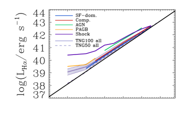
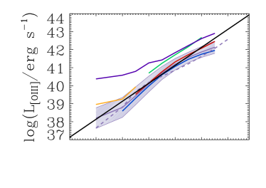
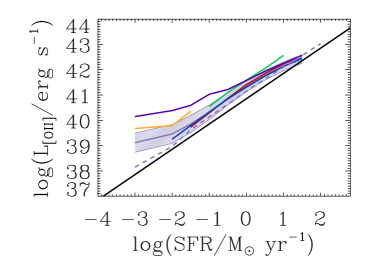
Figure 10: Average line luminosities of H$\alpha$, [O iii]$\lambda 5007$ and [O ii] $\lambda 3727$  (from top to bottom) in bins of SFR for TNG100 (solid mauve line with shaded 1$\sigma$ scatter) and TNG50 (dashed mauve line) galaxies at $z=0$. Relations for different galaxy types are also shown in the case of TNG100 (blue: SF-dominated; red: composite; green: AGN-dominated; orange: PAGB-dominated; lilac: shock-dominated). Also shown for completeness are relations often used in the literature (from Kennicutt et al. 1998 for H$\alpha$ and [O ii] $\lambda 3727$, and Sobral et al. 2015 for [O iii]$\lambda 5007$; black solid line in each panel). These should not be compared in detail with the IllustrisTNG predictions, as they were derived from purely solar-metallicity, SF-galaxy models assuming a Salpeter (1955) IMF truncated at 0.1 and 1M_⊙.

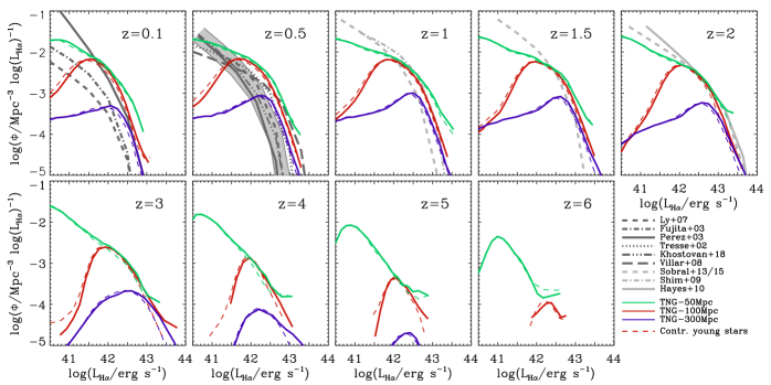
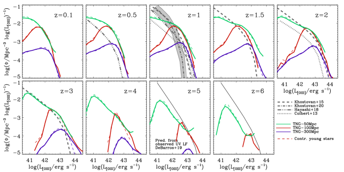
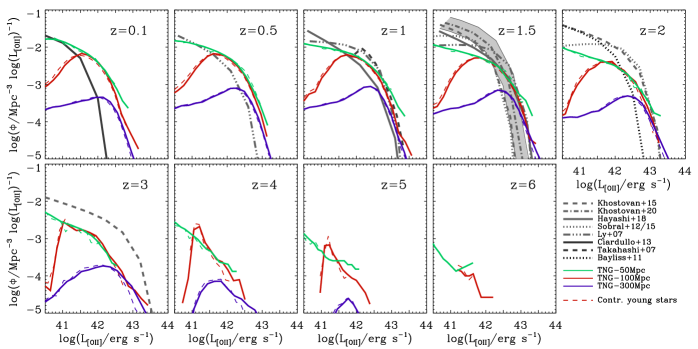
Figure 11: H$\alpha$- (top two rows), [O iii]+H$\beta$- (middle two rows) and [O ii]- (bottom two rows) luminosity functions of TNG50 (green solid lines), TNG100 (red solid lines) and TNG300 (lilac solid lines) galaxies more massive than $10^{8}\,\hbox{M${}_{\odot}$}$, $3\times 10^{9}\,\hbox{M${}_{\odot}$}$ and $10^{10}\,\hbox{M${}_{\odot}$}$, respectively, at $z=0.1,$ 0.5, 1, 1.5, 2, 3, 4, 5 and 6 (different panels, as indicated). Dashed coloured lines show the results obtained when considering only the contribution by H ii regions to the luminosity of each galaxy. Also shown are observational data from various sources listed in the legend (all corrected for attenuation by dust; different grey- and black-line styles). The peaks in the TNG100 and TNG300 luminosity functions arise from the resolution limits; galaxy number densities below the peak are incomplete and hence not meaningful.

4.1 Evolution of optical-line luminosity functions

4.1.1 Relation between H$\alpha$, [O iii]$\lambda 5007$and [O ii] $\lambda 3727$ luminosities and SFR for IllustrisTNG galaxies

We start by exploring how optical-line luminosities relate to the SFR for IllustrisTNG galaxies. Fig. 10 shows the mean relations between H$\alpha$, [O iii]$\lambda 5007$ and [O ii] $\lambda 3727$ luminosities (from top to bottom) and SFR for TNG100 and TNG50 galaxies at $z=0$ (solid and dashed mauve lines, respectively). In the case of TNG100, we distinguish between different types of galaxy populations (blue: SF-dominated; red: composite; green: AGN-dominated; orange: PAGB-dominated; lilac: shock-dominated). Also shown for completeness are relations often used in the literature (from Kennicutt et al. 1998 for H$\alpha$ and [O ii] $\lambda 3727$, and Sobral et al. 2015 for [O iii]$\lambda 5007$; black solid line in each panel). These should not be compared in detail with our predictions, as they were derived from purely solar-metallicity, SF-galaxy models assuming a Salpeter (1955) IMF truncated at 0.1 and 1M_⊙.

The good correlation between line luminosity and SFR for SF-dominated galaxies in Fig. 10 confirms that H$\alpha$, [O iii]$\lambda 5007$ and [O ii] $\lambda 3727$ can provide rough estimates of the SFR in such galaxies. For other galaxy types, contributions to line emission from an AGN, shocks and PAGB stars shift the relations to larger luminosities at fixed SFR. Hence, the ability to constrain galaxy type (Section 3.3) is important to refine SFR estimates from optical-line luminosities.

4.1.2 H$\alpha$ luminosity function

The top two rows of Fig. 11 show the evolution of the H$\alpha$ luminosity function of TNG50 (green lines), TNG100 (red lines) and TNG300 (lilac lines) galaxies over the redshift range $1\leq z\leq 6$ (different panels, as indicated). It is worth pointing out that the peaks in the TNG100 and TNG300 luminosity functions are an artefact of the resolution limit, which causes galaxy number densities below the peak to be incomplete and hence not meaningful. The highest resolution of the TNG50 simulation enables us to follow the evolution of the faint end down to luminosities below $\sim 10^{41}$ erg s^-1, and the larger cosmological volumes of the TNG100 and TNG300 simulations enable quantification of the evolution of the exponential cutoff at luminosities near $\sim 10^{43}$ erg s^-1.

At any redshift, the bulk of the H$\alpha$ luminosity in Fig. 11 arises from H ii regions ionized by young stars (coloured dashed lines). Only in the most luminous H$\alpha$ emitters, with $\hbox{$L_{\mathrm{H\alpha}}$}\ga 10^{43}$ erg s^-1, can the contribution from an AGN become significant. This makes the H$\alpha$ luminosity function a reliable tracer of the cosmic SFR density of galaxy populations, as often assumed in observational studies (e.g., Ly et al., 2007; Sobral et al., 2013; Sobral et al., 2015). In fact, Fig. 11 shows that, as a consequence of the rising cosmic SFR density of IllustrisTNG galaxy populations from $z=0.1$ to $z=3$, the simulated H$\alpha$ luminosity function strongly evolves over this redshift range: while the faint end hardly changes, the exponential cutoff rises from $\hbox{$L_{\mathrm{H\alpha}}$}\ga 10^{42}$ erg s^-1 to $\hbox{$L_{\mathrm{H\alpha}}$}\ga 10^{43}$ erg s^-1.

The predicted H$\alpha$ luminosity functions in Fig. 11 are in reasonable agreement with observational determinations (including corrections for dust attenuation) from various deep and wide, narrow-band and spectroscopic surveys conducted at $z<2$ (Tresse et al., 2002; Fujita et al., 2003; Villar et al., 2008; Shim et al., 2009; Hayes et al., 2010; Sobral et al., 2013; Sobral et al., 2015; Khostovan et al., 2018, shown as different grey lines). The large dispersion in these constraints illustrates the uncertainties inherent in their derivation (e.g., cosmic variance, corrections for dust attenuation, filter profile, completeness, etc.). In this respect, the constraints from the HiZELS survey (Sobral et al., 2013; Sobral et al., 2015, light-grey dashed lines) are of particular interest, as they provide homogeneous estimates of the H$\alpha$ luminosity function over the redshift range $1\leq z\leq 2$. These are consistent with the evolution predicted by our models, except at the faint end, where resolution effects and the stellar-mass cut at $10^{8}\,\hbox{M${}_{\odot}$}$ in the TNG50 simulation are likely to account for the shallower predicted slope.

At redshifts $z>2$, where future observational constraints will be gathered by JWST, Euclid and the Roman Space Telescope, the galaxy number density at fixed H$\alpha$ luminosity is predicted to strongly decline, e.g., by a factor of $\sim 30$ between $z=3$ and $z=6$ at $\hbox{$L_{\mathrm{H\alpha}}$}=10^{42}$ erg s^-1. While this reflects the decline of the cosmic SFR density over this redshift range in the IllustrisTNG simulations, these predictions should be taken with caution, because of the growing limitation by resolution effects affecting the census of small galaxies at high redshift.

4.1.3 [O iii]+H$\beta$ luminosity function

The middle two rows of Fig. 11 show the evolution of the [O iii]+H$\beta$ luminosity function of the TNG50, TNG100 and TNG300 galaxies, using the same layout as for the H$\alpha$ luminosity function in the top two rows. Here, the [O iii]+H$\beta$ luminosity is taken to be the sum of the [O iii]$\lambda 4346$, H$\beta$ and [O iii]$\lambda 5007$ luminosities, which are hard to separate in narrow-band surveys. We note that the predicted [O iii]+H$\beta$ luminosity function computed in this way differs noticeably from the pure [O iii]$\lambda 5007$ luminosity function only at the faint end.

As in the case of the H$\alpha$ line, Fig. 11 shows that the [O iii]+H$\beta$ luminosity function is dominated by H ii regions ionized by young stars at all redshifts. Only at $z=2$–3 do luminosities above $\hbox{$L_{\mathrm{[O\,\textsc{iii}]+H\beta}}$}\sim 10^{43.5}$ erg s^-1 start to be dominated by line emission from AGN. The [O iii]$\lambda 5007$+H$\beta$ luminosity function also exhibits strong evolution with redshift: even though the faint end hardly changes from $z=0.1$ to $z=3$, the exponential cutoff rises from $\hbox{$L_{\mathrm{[O\,\textsc{iii}]+H\beta}}$}\sim 10^{41.5}$ erg s^-1 at $z=0.1$ to $\hbox{$L_{\mathrm{[O\,\textsc{iii}]+H\beta}}$}>10^{43}$ erg s^-1 at $z=3$, in fair agreement with the bulk of observational constraints (Colbert et al., 2013; Hayashi et al., 2018; Khostovan et al., 2015, 2020).

The only constraint we could find on the [O iii]+H$\beta$ luminosity function at redshift $z>3$ is that derived indirectly from the UV luminosity function at $z=8$ by De Barros et al. (2019). For reference, we show this as a thin, black solid line in the $z=5$ and $z=6$ panels of the fourth row of Fig. 11. At $z=5$, our predictions are roughly consistent with this semi-empirical determination, which however lies $\sim 0.5\,$dex above the predictions at $z=6$. The difference could arise from uncertainties in the derivation of this indirect constraint, as well as from resolution effects in the simulations at that redshift.

4.1.4 [O ii] luminosity function

The evolution of the [O ii] $\lambda 3727$ luminosity function, shown in the bottom two rows of Fig. 11, has characteristics similar to that of the [O iii]+H$\beta$ luminosity function. It is largely dominated by the contribution from H ii regions ionized by young stars and shows strong evolution of the exponential cutoff, from $\hbox{$L_{\mathrm{[O\,\textsc{iii}]}}$}\sim 10^{42.5}$ erg s^-1 at $z=0.1$ to $\hbox{$L_{\mathrm{[O\,\textsc{iii}]}}$}\sim 10^{43}$ erg s^-1 at $z=2$. At redshifts $z=1$–1.5, the predicted evolution is in reasonable agreement with various empirical determinations (Khostovan et al., 2015, 2020; Hayashi et al., 2018; Sobral et al., 2015; Ly et al., 2007; Takahashi et al., 2007; Bayliss et al., 2011). At lower redshift, the number density of [O ii]-luminous emitters lies above those estimated by Ciardullo et al. (2013) and Ly et al. (2007), while at higher redshift, it lies below that estimated by Khostovan et al. (2015).

Overall, we conclude that the luminosity functions of the H$\alpha$, [O iii]+H$\beta$ and [O ii] emission lines predicted by the IllustrisTNG simulations are in reasonable agreement with empirical determination at redshifts from $z=0$ to $z=2$–3, although there are some discrepancies with the few existing constraints on the number densities of [O ii] $\lambda 3727$ emitters at $z<1$ and $z>1.5$.

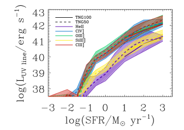
Figure 12: Average luminosities of different UV emission lines, He ii $\lambda 1640$, C iv $\lambda 1550$, O iii] $\lambda 1663$, Si iii] $\lambda 1888$ and C iii] $\lambda 1908$  (coloured as indicated) plotted against SFR for galaxies at redshifts $z=4$–7 in the TNG100 (solid lines for $\rm SFR\ga 10\,\hbox{M${}_{\odot}$}\,yr^{-1}$) and TNG50 (dashed lines, with shaded area indicating the 1$\sigma$ scatter) simulations.

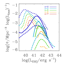
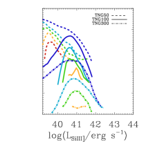
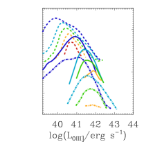
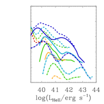
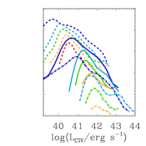
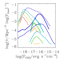
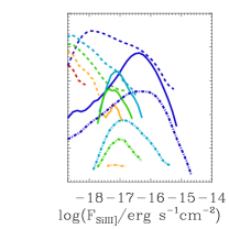
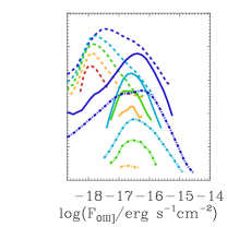
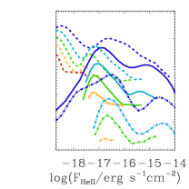
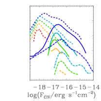
Figure 13: C iii] $\lambda 1908$, Si iii] $\lambda 1888$, O iii] $\lambda 1663$, He ii $\lambda 1640$ and C iv $\lambda 1550$  luminosity functions (panels from left to right, top row) and flux functions (bottom row) of TNG50 (dashed lines), TNG100 (solid lines) and TNG300 (dot-dashed lines) galaxies more massive than $10^{8}\,\hbox{M${}_{\odot}$}$, $3\times 10^{9}\,\hbox{M${}_{\odot}$}$ and $10^{10}\,\hbox{M${}_{\odot}$}$, respectively, at $z=2$, 4, 5, 6 and 7 (different colours, as indicated).

Two-hour exposure time

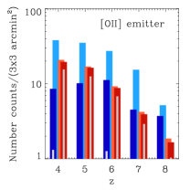
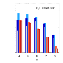
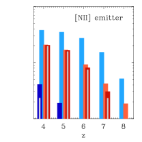
Five-hour exposure time

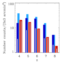
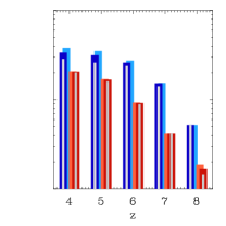
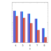
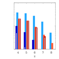
Ten-hour exposure time

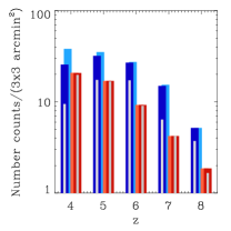
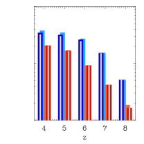
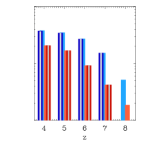
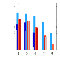
Figure 14: Number counts of [O ii] $\lambda 3727$, H$\beta$, [O iii]$\lambda 5007$, H$\alpha$ and [N ii]$\lambda 6584$ emitters (from left to right) as a function of redshift in a JWST/NIRSpec field of view ($3\times 3\ \mathrm{arcmin}^{2}$). The light blue and red bars, which are the same in all panels, show the number of, respectively, SF-dominated and active (AGN-dominated and composite) galaxies more massive than $10^{8}\,\hbox{M${}_{\odot}$}$ predicted in redshift bins centred on $z=4$, 5, 6, 7 and 8 by the TNG50 simulation (the fixed boxlength of the simulation translates into redshift-bin widths shrinking from $\Delta z=10^{-3}$ to $5\times 10^{-4}$ over this range). The dark blue and red bars show the subsets of these galaxies whose line emission can be detected with NIRSpec with 5$\sigma$ significance, assuming exposure times of 2, 5 and 10 hr (from top to bottom). The light-grey thin bars carved in the dark-colour bars show the effect of including dust attenuation with $A_{\rm V}=0.5$ and a Calzetti et al. (2000) curve.

4.2 Evolution of UV-line luminosity functions

Since UV emission lines become prominent in metal-poor galaxies and can be detected with JWST out to high redshifts (e.g., Stark et al., 2014), it is of interest to explore the predictions of our models for the evolution of UV-line luminosity and flux functions at $z\geq 2$. We can also investigate which UV lines potentially offer the best SFR estimators in high-redshift galaxies, at least when corrected for attenuation by dust, when standard (in particular, Balmer) optical lines fall out of the observational window.

Fig. 12 shows the relations between the average luminosities of different UV lines (lilac: He ii $\lambda 1640$; blue: C iv $\lambda 1550$; green: [O iii]$\lambda 5007$; yellow: Si iii] $\lambda 1888$; red: C iii] $\lambda 1908$) and SFR in the TNG100 and TNG50 galaxy populations (solid and dashed lines, respectively) over the redshift range $z=4$-7 (shaded, coloured areas show the 1$\sigma$ scatter about the TNG50 relations). All UV line luminosities appear to correlate with SFR over several orders of magnitude, the tightest relations being obtained for C iii] $\lambda 1908$, O iii] $\lambda 1663$, and Si iii] $\lambda 1888$  (1$\sigma$ scatter below 0.5 dex), compared to He ii $\lambda 1640$ and C iv $\lambda 1550$. This is because the latter two lines are more sensitive to contamination by an AGN component.

In the top row of Fig. 13, we show the luminosity functions of the C iii] $\lambda 1908$, Si iii] $\lambda 1888$, O iii] $\lambda 1663$, He ii $\lambda 1640$ and C iv $\lambda 1550$ emission lines for TNG50 (solid lines), TNG100 (dashed lines) and TNG300 (dot-dashed lines) galaxies at different redshifts from $z=2$ to $z=7$ (different colours, as indicated). As in the case of optical-line luminosity functions (Section 4.1), the TNG50, TNG100 and TNG300 simulations predominantly sample, respectively, the faint, intermediate and bright ranges of UV luminosity functions. In the luminosity ranges where predictions from different simulations overlap, these are in good general agreement, except for galaxies at $z\ga 6$, where the limitations arising from resolution effects become worse.

Regardless of the UV line considered, we find that at a given luminosity, the number density drops by up to an order of magnitude from $z=2$ to $z=6$, mainly for galaxies with luminosities below the exponential cutoff. Instead, the luminous end is largely in place as early as $z=6$, and thus evolves less strongly toward low reshift. The fact that the area under the luminosity function (i.e., the integrated luminosity function) decreases from $z=2$ to $z=7$ is a consequence of the decline in cosmic SFR density over this redshift interval, as shown by, e.g., Pillepich et al. (2018a).

It is interesting to note that the He ii $\lambda 1640$ and C iv $\lambda 1550$ luminosity functions exhibit bi-modal distributions. This is because, while the lower-luminosity peak is dominated by line emission from young star clusters, a second peak arises from the high He ii $\lambda 1640$ and C iv $\lambda 1550$ luminosities in AGN-dominated galaxies. This bi-modality is not observed in the other UV luminosity functions in Fig. 13, because C iii] $\lambda 1908$, Si iii] $\lambda 1888$ and O iii] $\lambda 1663$ require lower ionization energies, and hence, are less sensitive than He ii $\lambda 1640$ and C iv $\lambda 1550$ to the hard ionizing radiation from accreting BH.

As a complement to the rest-frame line-luminosity functions, we show in the bottom row of Fig. 13 the evolution of the associated line-flux functions, which are directly observable quantities. The observed-flux functions differ from the rest-frame luminosity functions because of the redshift-dependent luminosity distance. Although the main trends are similar to those described above for the luminosity functions, the main difference between flux and luminosity functions is the shift of the high-luminosity end toward lower relative fluxes at increasing redshift (since at fixed luminosity, the observed flux decreases with increasing redshift).

Overall, it will be instructive to explore the extent to which future observational studies at high redshift, for example with JWST/NIRSpec, will be consistent with the predicted optical/UV luminosity and flux functions in Figs 11 and 13, and whether potential inconsistencies between models and observations might require fundamental changes in models of galaxy evolution.

4.3 Predicted number counts in JWST/NIRSpec observations

The models presented in the previous sections allow us to predict the number of high-redshift galaxies that can be detected down to a given line-flux limit with the near-infrared spectrograph NIRSpec on JWST (Jakobsen et al., 2022). An interesting case study is that of the JWST Advanced Deep Extragalactic Survey (JADES), which combines NIRCam imaging and NIRSpec spectroscopy distributed in a ‘DEEP’ and ‘MEDIUM’ surveys (a guaranteed-time-observation program led by N. Lützgendorf and D. Eisenstein). Among the different components of JADES, we focus on the medium-resolution spectroscopy (resolving power $R\sim 1000$) that will be achieved on a few hundred galaxies in the DEEP survey (two NIRSpec pointings with exposure times of 8.4–25.2 ksec, i.e. from 2.3 to 7 hr, in each of several grating/filter configurations) and a few thousand galaxies in the MEDIUM survey (24 NIRSpec pointings with exposure times ranging from 2.7 to 9.3 ksec, i.e. 0.75 to 2.6 hr, per grating/filter configuration). We adopt the flux limits listed in Table 1, computed with the pre-flight JWST exposure-time calculator, for different lines at different redshifts and for different exposure times.

Two-hour exposure time

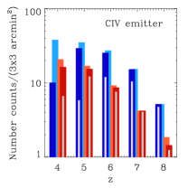
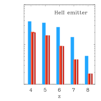
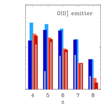
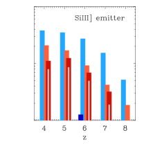
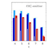
Five-hour exposure time

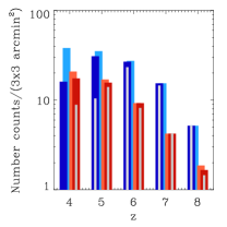
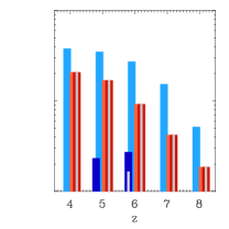
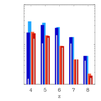
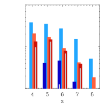
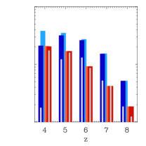
Ten-hour exposure time

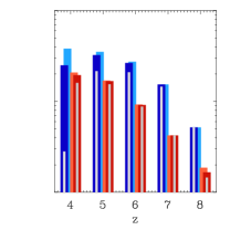
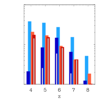
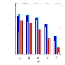
Figure 15: Same as Fig. 14, but for the C iv $\lambda 1550$, He ii $\lambda 1640$, O iii] $\lambda 1663$, Si iii] $\lambda 1888$ and C iii] $\lambda 1908$ emission lines. The predicted number counts of C iv $\lambda 1550$ emitters in the presence of dust are likely overestimated, as they ignore the effect of resonant scattering.

Line

$z=4$

$z=5$

$z=6$

$z=7$

$z=8$

Two-hour exposure time
[O ii] $\lambda 3727$ $-18.3$ $-18.5$ $-18.6$ $-18.6$ $-18.7$ H$\beta$ $-18.4$ $-18.6$ $-18.8$ $-18.8$ $-18.8$ [O iii]$\lambda 5007$ $-18.5$ $-18.6$ $-18.8$ $-18.8$ $-18.8$ H$\alpha$ $-18.7$ $-18.8$ $-18.8$ $-18.6$ – [N ii]$\lambda 6584$ $-18.7$ $-18.8$ $-18.8$ $-18.6$ – C iv $\lambda 1550$ $-17.4$ $-17.9$ $-18.1$ $-18.3$ $-18.4$ He ii $\lambda 1640$ $-17.5$ $-18.0$ $-18.2$ $-18.3$ $-18.4$ O iii] $\lambda 1663$ $-17.7$ $-18.0$ $-18.2$ $-18.3$ $-18.4$ Si iii] $\lambda 1888$ $-17.9$ $-18.2$ $-18.3$ $-18.4$ $-18.3$ C iii] $\lambda 1908$ $-17.9$ $-18.2$ $-18.3$ $-18.35$ $-18.3$ Five-hour exposure time
[O ii] $\lambda 3727$ $-18.5$ $-18.7$ $-18.8$ $-18.8$ $-19.0$ H$\beta$ $-18.8$ $-18.8$ $-19.0$ $-19.0$ $-18.9$ [O iii]$\lambda 5007$ $-18.8$ $-18.8$ $-19.0$ $-19.0$ $-19.0$ H$\alpha$ $-18.9$ $-19.0$ $-19.0$ $-18.8$ – [N ii]$\lambda 6584$ $-18.9$ $-19.0$ $-19.0$ $-18.8$ – C iv $\lambda 1550$ $-17.5$ $-18.0$ $-18.4$ $-18.5$ $-18.5$ He ii $\lambda 1640$ $-18.0$ $-18.4$ $-18.5$ $-18.5$ $-18.5$ O iii] $\lambda 1663$ $-17.8$ $-18.2$ $-18.4$ $-18.5$ $-18.5$ Si iii] $\lambda 1888$ $-18.0$ $-18.4$ $-18.5$ $-18.5$ $-18.5$ C iii] $\lambda 1908$ $-18.0$ $-18.4$ $-18.5$ $-18.5$ $-18.5$ Ten-hour exposure time
[O ii] $\lambda 3727$ $-18.6$ $-18.9$ $-19.0$ $-19.0$ $-18.9$ H$\beta$ $-18.9$ $-19.0$ $-19.1$ $-19.2$ $-19.1$ [O iii]$\lambda 5007$ $-19.0$ $-19.0$ $-19.1$ $-19.2$ $-19.1$ H$\alpha$ $-19.0$ $-19.2$ $-19.1$ $-18.8$ – [N ii]$\lambda 6584$ $-19.0$ $-19.2$ $-19.1$ $-19.0$ – C iv $\lambda 1550$ $-17.7$ $-18.2$ $-18.5$ $-18.6$ $-18.7$ He ii $\lambda 1640$ $-18.2$ $-18.5$ $-18.7$ $-18.7$ $-18.6$ O iii] $\lambda 1663$ $-17.9$ $-18.4$ $-18.5$ $-18.5$ $-18.7$ Si iii] $\lambda 1888$ $-18.2$ $-18.5$ $-18.7$ $-18.7$ $-18.6$ C iii] $\lambda 1908$ $-18.2$ $-18.5$ $-18.7$ $-18.7$ $-18.6$

Table 1: NIRSpec-specific flux-detection limits (in units of log[erg s^-1cm^-2]) for different optical/UV emission lines at redshifts z=4–8 for three different exposure times, as indicated. The 5$\sigma$ flux limits were computed with the pre-flight (version 1.3) of the JWST exposure-time calculator.

In this context, it is of interest to compute the number of galaxies expected to be detected in a given emission line, given an exposure time, in a NIRSpec field of view ($3\times 3\ \mathrm{arcmin}^{2}$). This is shown as a function of redshift in Fig. 14 for the [O ii] $\lambda 3727$, H$\beta$, [O iii]$\lambda 5007$, H$\alpha$ and [N ii]$\lambda 6584$ lines (from left to right), assuming exposure times of 2, 5 and 10 hr (from top to bottom). In each panel of Fig. 14, the light blue and red bars show the number of, respectively, SF-dominated and active (AGN-dominated and composite) galaxies more massive than $10^{8}\,\hbox{M${}_{\odot}$}$ predicted in redshift bins centred on $z=4$, 5, 6, 7 and 8 by the TNG50 simulation. The fixed boxlength of the simulation translates into redshift-bin widths shrinking from $\Delta z=10^{-3}$ to $5\times 10^{-4}$ over this range. These predicted numbers are the same in all panels of Fig. 14, independent of emission line and exposure time. In contrast, the dark blue and red bars show the subsets of these galaxies whose line emission can be detected with NIRSpec with 5$\sigma$ significance. These numbers change with emission line and exposure time.

So far, we have not considered attenuation of emission lines by dust, while galaxies may contain significant amounts of dust, even at early cosmic epochs (see e.g., Schneider et al., 2004; Zavala et al., 2022). We estimate the impact of attenuation by dust on the number counts of SF and active galaxies in Fig. 14 by adopting the dust attenuation curve of Calzetti et al. (2000) with a $V$-band attenuation of $A_{\rm V}=0.5\,$mag. The resulting drop in expected number counts is shown by the light-grey thin bars carved in the dark-colour bars.

Fig. 14 shows that the TNG50 simulation predicts from $\sim 40$ (20) SF-dominated (active) galaxies per NIRSpec field in the $z=4$ bin, to $\sim 5$ (2) at $z=8$. Virtually all of these can be detected in a two-hour exposure with NIRSpec in H$\alpha$ and [O iii]$\lambda 5007$, typically the brightest optical emission lines, out to $z=7$ (when H$\alpha$ drops out of the observational window) and $z=8$, irrespective of the presence of dust. Instead, exposures of at least 5 hours are required to achieve a nearly unbiased census of H$\beta$. Even 10-hour exposures will not be sufficient to achieve an unbiased census of [O ii] $\lambda 3727$ SF-dominated emitters, and even less so of [N ii]$\lambda 6584$ emitters, especially in the presence of attenuation by dust. At any of the survey depths in Fig. 14, the observed populations in these lines would be biased toward active galaxies.

All this suggests that the JADES/MEDIUM survey will be able to detect H$\alpha$ and [O iii]$\lambda 5007$ in the targeted galaxies out to $z=7$ and $z=8$, respectively, and the DEEP survey extend this to H$\beta$, while a substantial fraction of SF-dominated, [O ii] $\lambda 3727$ and [N ii]$\lambda 6584$ emitters might remain below the detectability limit of these surveys. It is also worth noting that some galaxies less massive than $10^{8}M_{\odot}$ may have line fluxes above the survey limits and therefore be detectable. As stated before, we do not consider such low-mass galaxies here as they are unresolved in TNG50.

In Fig. 15, we show the analogue of Fig. 14 for the C iv $\lambda 1550$, He ii $\lambda 1640$, O iii] $\lambda 1663$, Si iii] $\lambda 1888$ and C iii] $\lambda 1908$ UV emission lines (from left to right). If galaxies were dust-free, the most complete censuses in this wavelength range would be achievable for C iii] $\lambda 1908$, O iii] $\lambda 1663$ and C iv $\lambda 1550$ emitters at $z\ga 6$, especially for long exposure times, although significant fractions of SF-dominated galaxies would still be missed at lower redshifts. Instead, the weaker He ii $\lambda 1640$ and Si iii] $\lambda 1888$ lines can be properly sampled only in active galaxies, because He ii $\lambda 1640$ requires highly energetic photons, while Si iii] $\lambda 1888$, hindered by the low abundance of Si relative to C and O, is boosted by AGN radiation. Exposure times of at least 5 hours would be required to start detecting populations of dust-free, SF-dominated emitters in these lines with NIRSpec, and even 10 hours would not suffice to achieve proper censuses of these populations.

In the presence of dust, the expected number counts in Fig. 15 drop significantly, particularly for SF-dominated galaxies, whose weaker lines compared to AGN-dominated galaxies fall more easily below the detectability limits of surveys. Yet, significant fractions of C iii] $\lambda 1908$, O iii] $\lambda 1663$ and C iv $\lambda 1550$ emitters still appear detectable with the adopted $A_{\rm V}=0.5$, at least for exposure times exceeding 10 hours. We caution however that the predicted counts of C iv $\lambda 1550$ emitters are likely to be overestimated, as we have ignored the enhanced absorption of C iv $\lambda 1550$ photons by dust due to resonant scattering (e.g., Senchyna et al., 2022).

The results of Fig. 15 therefore suggest that the UV lines most accessible to the JADES/MEDIUM and DEEP surveys, modulo dust attenuation, are likely to be C iii] $\lambda 1908$ and O iii] $\lambda 1663$, and, in cases where enhanced attenuation by resonant scattering is particularly modest, C iv $\lambda 1550$. SF-dominated He ii $\lambda 1640$ and Si iii] $\lambda 1888$ emitters are likely to remain more elusive. While this prediction relies on SF models having difficulty to reproduce the observed He ii $\lambda 1640$ emission of low-redshift analogues of distant SF galaxies (e.g., Plat et al., 2019), it is interesting to note that a non-detection of He ii $\lambda 1640$ combined with detections of C iii] $\lambda 1908$ and O iii] $\lambda 1663$ (and perhaps C iv $\lambda 1550$) could point to a population of SF-dominated galaxies (as expected from the He ii $\lambda 1640$-based diagnostic diagrams in Fig. 9).

5 Discussion

In Sections 3 and 4, we have shown that the predicted optical and UV emission-line properties of the IllustrisTNG galaxy populations are consistent with numerous observational constraints out to redshifts $z\sim 2$–3. Based on this success, we could make predictions about the observability of these lines in more distant galaxies, out to $z\sim 7$–8, and propose associated spectral diagnostics as guidance for the interpretation of new spectroscopic surveys at high redshift. These results represent a major statistical extension of earlier work by Hirschmann et al. (2017); Hirschmann et al. (2019).

Despite this success, the emission-line catalogues of IllustrisTNG galaxies used in our study may be affected by several caveats related to current photoionization models, modern cosmological simulations and our coupling methodology. We discuss these in Sections 5.1 and 5.2 below and also compare in Section 5.3 our emission-line catalogues to those from previous studies of optical and UV emission lines of simulated galaxies.

5.1 Caveats in the photoionization models

All photoionization models considered in this work were performed with recent versions of the Cloudy and Mappings photoionization codes, adopting a common set of element abundances down to metallicities of a few per cent solar (Section 2.2). However, these models are computed via 1D calculations of a gas patch irradiated by ionizing photons, assuming a simplified geometry (e.g., spherical, plane-parallel) and constant gas density, which do not reflect the complex 3D gas distributions found in nature. Also, while the H ii-region and AGN-NLR photoionization models employed here are ionization-bounded, some actively star-forming galaxies show evidence of leakage of Lyman-continuum photons (e.g., de Barros et al., 2016; Shapley et al., 2016; Bian et al., 2017; Flury et al., 2022). This generally tends to reduce the intensities of low-ionization relative to high-ionization lines (see, e.g., the density-bounded calculations of Plat et al., 2019).

The PAGB models we adopted to describe gas photoionized by evolved stellar populations also suffer from uncertainties. In particular, the most recent version of the Bruzual & Charlot (2003) stellar-population-synthesis code we rely on incorporates PAGB evolutionary tracks from Miller Bertolami (2016), which have significantly shorter lifetimes – although compensated in part by higher luminosities – than previous prescriptions. Adopting older PAGB models could enhance the predicted EW(H$\alpha$) of PAGB-dominated galaxies by a factor of up to 2. We have checked that this would not qualitatively affect our results (in the sense that more galaxies would be PAGB-dominated, but they would still separate robustly in the WHAN diagram of Fig. 3). For the ionizing radiation from an accreting black hole in the AGN-NLR models, for simplicity, we adopted the fixed broken power-law shape described by Feltre et al. (2016), with $S_{\nu}\propto\nu^{\alpha}$ and $\alpha=-1.7$ at wavelengths below 2500 Å. As shown by Hirschmann et al. (2017); Hirschmann et al. (2019), adopting a different value for $\alpha$ would not significantly affect the predicted luminosities of the optical and UV emission lines considered in the present work.

Another, perhaps more serious limitation of the H ii-region and PAGB models used in our study is that they do not include the hot ionizing radiation from binary-star products (envelope-stripped or spun-up stars), as they are based on single-star population-synthesis models. Hard radiation from binary stars will enhance the luminosities of lines from species requiring very high ionizing energies, such as He ii (see, e.g., Xiao et al., 2018). This point is of particular relevance, as no current stellar-population-synthesis model can account for the strong He ii $\lambda 1640$ and He ii $\lambda 4686$ emission exhibited by some very metal-poor ($\la 0.2\,\hbox{Z${}_{\odot}$}$) SF galaxies (see, e.g., Plat et al., 2019; Stanway & Eldridge, 2019). In fact, this is true even for the BPASS v2.2.1 models of Eldridge et al. (2017), which do include binary-star populations. Interestingly, the latest version of the Bruzual & Charlot (2003) single-star models used here, which incorporate updated calculations of stellar evolution and atmospheres (Bressan et al., 2012; Chen et al., 2015), produce more He ii-ionizing photons than BPASS v2.2.1 (see Plat et al., 2019). Other potential sources of He ii emission in such metal-poor galaxies could be mini-AGN, radiative shocks and massive X-ray binaries, although these are heavily debated (e.g., Plat et al., 2019; Senchyna et al., 2020; Simmonds et al., 2021; Umeda et al., 2022).

Despite the above caveats, the predictions of the H ii-region and AGN-NLR models used in this study have been repeatedly shown to perform remarkably well in comparisons with observations of common emission lines from other elements than He ii (e.g., Chevallard et al., 2018; Mignoli et al., 2019; Tang et al., 2019). As shown in Section 3.5, increasing the He ii $\lambda 1640$-line luminosity predicted by our H ii-region models by a factor of 4 of would not reduce much the effectiveness of the suggested selection criteria in UV diagnostic diagrams in Fig. 9 (in line with the result of Hirschmann et al., 2019). We also find that this would attenuate the bi-modality of the He ii $\lambda 1640$-luminosity function (Fig. 13) and increase the number counts of SF-dominated, He ii $\lambda 1640$ emitters by a factor of 2 to 3 (Fig. 15).

Finally, we note that the radiative-shock models of Alarie & Morisset (2019) used in this study update the older calculations of Allen et al. (2008), which were based on a previous version of the Mappings code and spanned a smaller range of metallicities. Both model sets are limited to shocks fast enough ($\geq 100\,$km s^-1) to generate sufficient radiation to ionize the pre-shock gas before it enters the shock front (i.e., to allow the pre-shock gas to reach ionization equilibrium before it is shocked; see also Sutherland & Dopita, 2017). The models also assume that shocks are propagating in a neutral medium ionized by the hot post-shock gas, which might not always be the case in practice (e.g., if a shock propagates through an ionized medium). As we shall see in the next section, the resolution and identification of shocks in cosmological simulations tend to include stronger assumptions and limitations than do the grids of radiative-shock models.

5.2 Caveats in the IllustrisTNG simulations and their coupling with emission-line models

A potential source of inaccuracy of all current large-scale cosmological simulations, including IllustrisTNG, is that they do not resolve the ISM, which forces one to appeal to often simplified and ad-hoc sub-resolution models to describe baryonic processes (see Naab & Ostriker, 2016, for a discussion). Specifically, the choice of stellar- and AGN-feedback models has been shown to significantly affect various galaxy properties (e.g. Pillepich et al., 2018b). In this context, it is important to stress that IllustrisTNG is one of the best-tested and explored, large-scale cosmological simulations to date, providing fairly realistic galaxy populations up to $z=3$, for example in terms of chemical enrichment, SFR and black-hole accretion-rate histories (although the observed AGN luminosity function is not always well reproduced, especially at low redshift, see Habouzit et al., 2019, 2022), stellar populations and the associated scaling relations. This success provides a solid foundation for our predictions of the emission-line luminosities controlled by these physical quantities.

Furthermore, because IllustrisTNG, like other modern large-scale cosmological simulations, does not resolve gas properties, such as density, in individual ionized regions, nor does it track the formation, evolution and destruction of dust grains in the ISM, we must adopt a fixed hydrogen gas density in ionized regions ($10^{3}\,$cm^-3 for NLR, $10^{2}\,$cm^-3 for H ii regions and $10\,$cm^-3 for line emission from post-AGB stars), as well as a fixed dust-to-metal mass ratio ($\xi_{d}=0.3$). As described in section 5.1.4 of Hirschmann et al. (2017), both recent observations (De Cia et al., 2016; Wiseman et al., 2017) and semi-analytic models (Popping et al., 2016) suggest that, at given gas metallicity, the dust-to-metal mass ratio hardly changes with redshift out to $z=6$. The models further predict that this is the case also at fixed stellar mass (see figs 5 and 6 of Popping et al., 2016) and that galaxies more massive than $M_{\mathrm{stellar}}>3\times 10^{9}M_{\odot}$ are expected to have dust-to-metal mass ratios around 0.2, reasonably close to our adopted value. In Hirschmann et al. (2017); Hirschmann et al. (2019), we further studied the impact of these parameters on optical and UV line ratios, and found that they have a smaller effect on observed line ratios than the parameters of the photoionization models that can be determined from the simulations.

Another consequence of not resolving individual H ii regions in IllustrisTNG is that we have to adopt galaxy-wide properties of H ii-regions. We follow here the methodology of Charlot & Longhetti (2001, see Section 2 above), which convolves the time evolution of an H ii region with the galaxy star-formation history. While this approach goes beyond most current photoionization models (which typically treat a galaxy as a single region ionized by the entire stellar population), it suffers from shortcomings: even though we assume that a galaxy is composed of several H ii regions (with different star-cluster ages), any variation in the gas properties of the regions across the galaxy (such as density, filling factor and metallicity) is neglected. Regardless, these galaxy-wide line-emission models may be justified by their long-term success in reproducing observed galaxy spectra (Section 5.1). More detailed studies will be needed to fully validate this approach, but they lie beyond the scope of the present paper.

Furthermore, the inability to resolve the ISM in large-scale cosmological simulations such as IllustrisTNG implies that shocks cannot be tracked and identified in unresolved cool gas phases. In fact, the on-the-fly shock finder described in Section 2 is by default disabled for star-forming gas. We have therefore intentionally neglected shock-related emission from the dense star-forming ISM itself, which could arise for example from supernova explosions. Instead, in IllustrisTNG, we are primarily capturing shocks caused by (AGN-driven) outflows, gas accretion as well as merger events arising in the warm/hot component of the ISM and in more distant regions, such as the disk-halo interface. Thus, in our analysis, we cannot draw any robust conclusion on line emission due to shocks in higher-redshift galaxies, where AGN-driven outflows seem to be less prevalent, and instead shocks due to stellar feedback, neglected in our approach, may become important. Also, at the moment, IllustrisTNG includes radiation-driven feedback only as thermal energy input, which may be insufficient to describe reality. We might therefore miss shocks linked to radiation-driven winds from radiatively efficient AGN, which may become particularly important in high-redshift galaxies.

While our modelling of synthetic emission lines of IllustrisTNG galaxies accounts for the effects of dust in H ii regions and AGN NLR (Section 2.3), it neglects attenuation by dust in the diffuse ISM (with the exception of Figs 14 and 15 in Section 4.3). To some extent, this neglect is justified by the fact that we compare our models with observed line ratios and line-luminosity functions corrected for this effect. Moreover, as expected from our results in section 5.1 of Hirschmann et al. (2019), we find that adopting a Calzetti et al. (2000) attenuation law with a $V$-band attenuation of $A_{V}=0.5\,$mag would negligibly impact most UV diagnostic diagrams in Fig. 9. This however would reduce the predicted number counts of line emitters at high redshift by factors of up to several, as shown by Figs 14 and 15. A more sophisticated modelling of dust (in the spirit of the on-the-fly dust modelling of McKinnon et al., 2018), beyond the scope of the present paper, will be required for more robust predictions.

Finally, we note that our methodology does not account for the effect of interstellar-line absorption in stellar birth clouds nor in the diffuse ISM. As shown by Vidal-García et al. (2017), while some prominent UV emission lines, such as O iii] $\lambda 1663$, Si iii] $\lambda 1888$ and C iii] $\lambda 1908$, are little sensitive to interstellar absorption, the luminosities of other lines, such as C iv $\lambda 1550$ and N v $\lambda 1240$, can be significantly reduced through this effect. While quantifying interstellar-line absorption in simulated galaxies is important, we postpone such a complex analysis to a future study.

5.3 Comparison with previous emission-line studies

In recent years, an increasing number of theoretical studies have emerged, which provide models for the nebular emission from young star clusters in galaxies in cosmological simulations. Below, we briefly outline the different methodologies proposed to compute line emission, summarise the main associated goals and results, and discuss how they compare with the method and analysis presented in this work.

The Sags semi-analytic model (Orsi et al., 2014): In this work, the gas metallicity and ionization parameter (via a dependency on gas metallicity) of Sags galaxies are used to select H ii-region models from a Mappings iii library (Levesque et al., 2010). With this method, the authors reproduce the local BPT diagram and the evolution of optical-line luminosity functions (we note that the predicted [O ii] $\lambda 3727$-luminosity function underestimates the observed one locally, as for our models in Fig. 11). However, their BPT diagrams, specifically the [O iii]/H$\beta$-ratio, do not evolve with redshift as observed. This model has been further applied to the Galacticus and Sage semi-analytic models (run over merger trees from the MultiDark simulation) to explore the luminosity functions and clustering of [O ii] $\lambda 3727$-emitting galaxies (Favole et al., 2020).

The Sage semi-analytic model applied to the UNIT project simulations (Knebe et al., 2022): Emission lines for the Sage semi-analytic model are constructed using the same method as in Orsi et al. (2014). Thanks to the large volume of the UNIT simulation (effectively $\sim 5\,$Gpc³), this study presents galaxy catalogues for Euclid forecasts. The authors start by validating their model against the observed H$\alpha$ luminosity function, and then explore the abundance and clustering of model H$\alpha$-emitting galaxies.

The Galacticus semi-analytic model (Zhai et al., 2019): The emission-line luminosities of Galacticus galaxies are computed using the Cloudy photoionization code (Ferland et al., 2013). The key step is to generate and interpolate tabulated libraries of emission-line luminosities using Cloudy as a function of the number of ionizing photons for various species, the ISM metallicity, the hydrogen gas density and the volume filling factor of H ii regions, which can be computed for Galacticus galaxies. The authors validate their emission-line results against observed H$\alpha$ and [O iii]$\lambda 5007$ luminosity functions and make predictions of number counts of line-emitting galaxies for galaxy surveys with the Roman Space Telescope.

The L-Galaxies semi-analytic model (Izquierdo-Villalba et al., 2019): This study adds the Orsi et al. (2014) model to L-Galaxies lightcones (run over the Millennium simulation) to create synthetic galaxy catalogues including emission lines for narrow-band photometric surveys. The authors focus on optical lines (including [Ne iii]$\lambda\lambda 3869,3967$) and find fairly good agreement with the observed evolution of the H$\alpha$, [O iii]$\lambda 5007$ and [O ii] $\lambda 3727$ luminosity functions.

The Galform semi-analytic model (Gonzalez-Perez et al., 2018, 2020; Baugh et al., 2022): Gonzalez-Perez et al. (2018, 2020) assign H ii-region models from Stasińska (1990) to Galform galaxies and investigate line-luminosity functions, halo-occupation distributions and the distribution of these galaxies in the cosmic web. While the original Galform emission-line model provided a poor reproduction of local BPT diagrams, Baugh et al. (2022) propose an updated model based on the published version of the Gutkin et al. (2016) photoionization grid and a relation between ionization parameter, gas metallicity, gas density and specific SFR from Kashino & Inoue (2019). Their study suggests that the offset in [O iii]/H$\beta$ of high-redshift relative to local galaxies results primarily from a higher ionization parameter and higher gas density, largely in line with our results in Hirschmann et al. (2017) and in Section 3.3 above.

The $z>7$ cosmological simulation of Shimizu et al. (2016): This study explores the optical- and UV-line emission of $z>7$ galaxies in cosmological simulations and their detectability with different current and future observational facilities (JWST, extremely large telescopes). The authors compute Ly$\alpha$, H$\alpha$ and H$\beta$ line luminosities using Pegase 2 (Fioc & Rocca-Volmerange, 1997). The luminosities of metal lines are scaled to the H$\beta$ luminosity based on Cloudy models and assuming a metallicity-dependent emission efficiency for each line. Shimizu et al. (2016) find that [O iii]$\lambda 5007$, H$\beta$, C iv $\lambda 1550$ and C iii] $\lambda 1908$ are the brightest lines in high-redshift galaxies and suggest that these could be strong targets for future observational facilities out to even for $z\sim 15$.

The Simba cosmological simulation (Garg et al., 2022): In this study, the nebular emission of a simulated galaxy is computed by summing the contributions from all young-star particles. The authors employ a sub-grid model to describe the star-cluster mass distribution per star particle and perform Cloudy calculations, using ages and metallicities appropriate for each star particle, as well as an empirical dependence of N/O on O/H (in the spirit of CloudyFSPS, Byler et al., 2017). Even though this methodology provides spatially-resolved information about line emission in a galaxy, it neglects all important dust processes in H ii regions (van Hoof et al., 2004). With this approach, Garg et al. (2022) reproduce the star-forming branch of the local BPT diagram and find that the [O iii]/H$\beta$ offset at high redshift arises primarily from selection effects. Yet, they find a mismatch between the predicted and observed [O iii]/H$\beta$ ratios of $z\sim 2$ galaxies, which can be alleviated by invoking higher N/O ratio or a lower ionization parameter at fixed O/H ratio at high redshift. While Hirschmann et al. (2017) had a similar conclusion with regard to N/O, the finding of Garg et al. (2022) concerning the ionization parameter disagrees with our result in Section 3.3 above, as well as with those of several previous studies (e.g., Brinchmann et al., 2008; Hirschmann et al., 2017; Kashino et al., 2017; Kewley et al., 2019; Baugh et al., 2022).

The BlueTides cosmological simulation at $z=8-13$ (Wilkins et al., 2020): As in the Simba simulation of Garg et al. (2022), the nebular emission of a simulated galaxy is computed by summing the contributions from all young-star particles, connecting ionization-bounded Cloudy models to the predicted gas metallicity and ionization parameter of each star particle, and assuming a fixed gas density and dust-to-metal mass ratio. The authors focus on predictions of a few optical (H$\alpha$, H$\beta$ and [O iii]$\lambda 5007$) and UV (C ii] $\lambda 2326$, C iii] $\lambda 1908$ and [Ne iii]$\lambda\lambda 3869,3967$) emission lines for simulated galaxies at $z=8$–13. They find good agreement of the predicted equivalent-width distributions of C iii] $\lambda 1908$ and [O iii]$\lambda 5007$+H$\beta$ with the few available observational constraints, but poorer agreement between the predicted and observed (from de Barros et al., 2016) [O iii]$\lambda 5007$+H$\beta$ luminosity function. As we have seen, at slightly lower redshift ($z=5$–6), our predicted [O iii]+H$\beta$ luminosity function based on the IllustrisTNG simulations roughly matches this observational constraint (Fig. 11).

The IllustrisTNG cosmological simulation at high redshifts (Shen et al., 2020): In this work, the H$\alpha$, H$\beta$ and [O iii]$\lambda 5007$ luminosities of IllustrisTNG galaxies at $z=2$–8 are computed through the coupling with a Mappings iii library of young ionizing stars clusters (Groves et al., 2008, considering only stellar age and metallicity for the coupling, and including dust physics). The authors find that the predicted [O iii]$\lambda 5007$+H$\beta$ luminosity function is consistent with observations at $z=2$–3, but that the H$\alpha$ luminosity function at $z\sim 2$ is $\sim 0.3$ dex dimmer than observed. At higher redshift, the models show hardly any evolution of the luminosity functions out to $z\sim 5$, and are slightly dimmer than the observed [O iii]$\lambda 5007$+H$\beta$ luminosity of De Barros et al. (2019). In contrast, as illustrated by Fig. 11 above, our emission-line treatment of the same cosmological simulations allows us to capture the observed H$\alpha$ luminosity function of $z=2$ galaxies, and we find a marked decline of the H$\alpha$ and [O iii]+H$\beta$ luminosity functions from $z=3$ to $z=6$. These contradictory emission-line predictions will be testable with upcoming JWST surveys.

To summarise, the vast majority of recent studies on emission-line predictions of simulated galaxies focus on optical-line luminosity functions, clustering of line emitters and number-count predictions for high-redshift galaxy surveys expected to emerge from current and future observational facilities. Despite the wide variety of modelling approaches, and the differences in photoionization models, basic predictions, such as optical-line luminosity functions are (surprisingly) widely consistent across different studies, including the work presented here. Only two such published studies (Garg et al., 2022; Baugh et al., 2022, aside from our own previous work) explored the location of simulated galaxies in BPT diagrams, and the evolution of the associated line ratios with redshift. The results of Baugh et al. (2022) agree with those presented here (and in Hirschmann et al., 2017) by favouring an evolution of the ionization parameter as the main driver of the rise in [O iii]/H$\beta$ ratio at high redshift, in stark contrast to the theoretical results of Garg et al. (2022), which instead favour selection effects as an explanation for the observed trends.

Compared to the above previous studies, our approach is unique in that we consider a large parameter space of physical quantities, as well as a more self-consistent modelling of the ionization parameter to select H ii-region photoionization models. Even though in some cosmological simulations, line emission is modelled on a spatially resolved basis, it is not clear how much more reliable such an approach is than the one presented here: modern, large-scale cosmological simulations can by no means resolve ionized regions in the ISM and masses of young star clusters, so that additional assumptions/sub-grid models become necessary (often just considering star-particle age and metallicity to model line emission).

Most importantly, we account not only for stellar nebular emission of simulated galaxy populations, as done in literature so far, but also simultaneously for line emission due to AGN, post-AGB stars and fast radiative shocks, resulting in comprehensive emission-line galaxy catalogues at different cosmic epochs.

6 Summary

In this paper, we have presented the first multi-component, optical and UV emission-line catalogues of large simulated galaxy populations at different cosmic epochs. Following the methodology of Hirschmann et al. (2017); Hirschmann et al. (2019), the emission-line catalogues have been constructed by employing the IllustrisTNG cosmological simulations and by self-consistently connecting them to modern, state-of-the-art photoionization models (Gutkin et al., 2016; Feltre et al., 2016; Hirschmann et al., 2017; Alarie & Morisset, 2019). This allows us to compute in a self-consistent way the line emission from multiple components: young star clusters, AGN NLR, PAGB stellar populations and, for the first time, fast radiative shocks. Specifically, we consider predictions from IllustrisTNG galaxies for the redshift evolution of global and central interstellar metallicity, C/O abundance ratio, SFR, BH accretion rate, global and central average gas densities, the age and metallicity of PAGB stellar populations, and shock properties (velocity, magnetic-field strength, interstellar metallicity and shock surface). Based on these, we select SF, AGN, PAGB and shock nebular-emission models for each simulated galaxy (above the mass-resolution limit) at any redshift. By default, we adopt a fixed dust-to-metal mass ratio, ionized-gas hydrogen density, power-law index of the AGN ionizing radiation and pre-shock gas density.

Taking advantage of these emission-line catalogues of IllustrisTNG galaxy populations, we have presented a variety of optical and UV diagnostic diagrams to identify ionizing sources in galaxies in the local Universe and at high redshift, together with the predicted evolution of line-luminosity functions and number counts of distant line-emitting galaxies expected to be detectable in deep spectroscopic observations with the NIRSpec instrument on board JWST. We can summarise our main results as follows:

• The synthetic [O iii]/H$\beta$, [N ii]/H$\alpha$, [S ii]/H$\alpha$, [O i]/H$\alpha$ and [O iii]/[O ii] emission-line ratios and H$\alpha$ equivalent widths of IllustrisTNG galaxies are in excellent statistical agreement with observations of star-forming, active, shock-dominated and retired (PAGB) SDSS galaxies in the local Universe. This confirms, for large galaxy populations (and with the different physical models adopted), the result originally obtained by Hirschmann et al. (2017); Hirschmann et al. (2019) for only 20 re-simulated, massive galaxies.

• Our results are consistent with the classical selection criteria in standard BPT diagnostic diagrams to distinguish SF and active galaxies in the local Universe. Furthermore, we confirm that the WHAN diagram can robustly identify retired galaxies, and the [O iii]/[O ii]-versus-[O i]/H$\alpha$ diagram shock-dominated galaxies.

• Present-day galaxies classified as ‘SF-dominated’ and ‘composites’ (i.e., SF+AGN) are found to be primarily star-forming, main-sequence galaxies with large cold-gas fractions. Then, SFR and cold-gas content successively decrease from ‘AGN-dominated’ to ‘shock-dominated’ and ‘PAGB-dominated’ galaxies: shock-dominated galaxies are predominantly located in the green valley of the SFR-stellar mass plane, and PAGB-dominated galaxies on the red sequence. This is primarily due to AGN feedback causing shocks in outflowing gas and suppressing star formation and black-hole accretion. This allows the (intrinsically weak) line emission from shocks and PAGB stars to become dominant.

• Shock- and PAGB-dominated galaxies make up between 3 and 10 per cent of the present-day galaxy population, depending on box size and resolution of the simulation. At redshifts $z>1$, these fractions drop below 1 per cent, with SF-dominated galaxies being the most abundant population (between 40 and 70 per cent) at all redshifts.

• At fixed [N ii]/H$\alpha$ ratio, the [O iii]/H$\beta$ ratio is predicted to increase from low to high redshift. For SF-dominated galaxies, the increase is similar to that reported in several observational studies (e.g., Steidel et al., 2014). We confirm our previous finding in Hirschmann et al. (2017) that at fixed galaxy stellar mass, the increase in [O iii]/H$\beta$ from low to high redshift is primarily a consequence of a higher ionization parameter in high-redshift galaxies, regulated by a larger specific SFR and a higher global gas density (consistent with the results of Baugh et al., 2022).

• At high redshifts, classical optical-selection criteria to identify the dominant ionizing sources in galaxies are no longer applicable: a drop in [N ii]/H$\alpha$ causes composite and AGN-dominated galaxies to shift toward the SF-dominated region of the classical [O iii]/H$\beta$-versus-[N ii]/H$\alpha$ BPT diagram. Instead, nine UV diagnostic diagrams and related selection criteria, originally presented in Hirschmann et al. (2019, for 20 re-simulated massive galaxies and their progenitors), provide a powerful means to distinguish SF from active galaxy populations out to early cosmic times (e.g., C iii] $\lambda 1908$/He ii $\lambda 1640$ versus O iii] $\lambda 1663$/He ii $\lambda 1640$).

• The synthetic emission-line properties of IllustrisTNG galaxies can largely reproduce the observed evolution of the H$\alpha$, [O iii]$\lambda 5007$ and [O ii] $\lambda 3727$ luminosity functions out to $z=3$ (albeit with some tension for [O ii] $\lambda 3727$). We provide predictions of optical- and UV-line luminosity and flux functions at $z>3$, potentially useful for future surveys with, e.g., JWST, Euclid and the Roman Space Telescope. From $z=3$ to $z=7$, the predicted number densities of optical and UV emission-line galaxies can drop by up to three orders of magnitude (primarily at faint luminosities), reflecting the declining SFR density over that redshift range.

• Finally, we present number counts of SF and active galaxies expected to be detectable at redshifts between $z=4$ to $z=8$ in deep, medium-resolution spectroscopic observations with the NIRSpec instrument on board JWST. We find that 2-hour-long exposures are sufficient to obtain unbiased censuses of H$\alpha$ and [O iii]$\lambda 5007$ emitters, while at least 5 hours are required for H$\beta$, irrespective of the presence of dust. Instead, for [O ii] $\lambda 3727$, O iii] $\lambda 1663$, C iii] $\lambda 1908$, C iv $\lambda 1550$, [N ii]$\lambda 6584$, He ii $\lambda 1640$ and Si iii] $\lambda 1888$  emitters, even though the active-galaxy population can still be well sampled, progressively smaller fractions of the SF-galaxy population are likely to be detectable, especially in the presence of dust, even with exposure times exceeding 10 hours.

Overall, the multi-component optical and UV emission-line galaxy catalogues presented in this paper include for the first time not only stellar nebular emission of simulated galaxy populations, as done in literature so far, but also simultaneously line emission due to AGN, post-AGB stars and fast radiative shocks. These catalogues provide useful insights into various diagnostic diagrams and statistical properties of optical and UV emission-line galaxies. These mock observables may be further helpful for the interpretation of near- and far-future emission-line surveys with, e.g., JWST, Euclid and the VLT/MOONs. This study is the first of a series, in which we also plan to explore, for example, the clustering of emission-line galaxies and the use of strong-line ratios as tracers of interstellar metallicity, the ionization parameter and other physical quantities of the ISM in high-redshift galaxies.

References

- Alarie & Morisset (2019) Alarie A., Morisset C., 2019, Rev. Mex. Astron. Astrofis., 55, 377
- Allen et al. (2008) Allen M. G., Groves B. A., Dopita M. A., Sutherland R. S., Kewley L. J., 2008, ApJS, 178, 20
- Baldwin et al. (1981) Baldwin J. A., Phillips M. M., Terlevich R., 1981, PASP, 93, 5
- Baugh et al. (2022) Baugh C. M., Lacey C. G., Gonzalez-Perez V., Manzoni G., 2022, MNRAS, 510, 1880
- Bayliss et al. (2011) Bayliss K. D., McMahon R. G., Venemans B. P., Ryan-Weber E. V., Lewis J. R., 2011, MNRAS, 413, 2883
- Belfiore (2016) Belfiore F. e. a., 2016, MNRAS, 461, 3111
- Berg et al. (2018) Berg D. A., Erb D. K., Auger M. W., Pettini M., Brammer G. B., 2018, ApJ, 859, 164
- Bian et al. (2017) Bian F., Fan X., McGreer I., Cai Z., Jiang L., 2017, ApJ, 837, L12
- Blanton et al. (2017) Blanton M. R., et al., 2017, AJ, 154, 28
- Bressan et al. (2012) Bressan A., Marigo P., Girardi L., Salasnich B., Dal Cero C., Rubele S., Nanni A., 2012, MNRAS, 427, 127
- Brinchmann et al. (2008) Brinchmann J., Pettini M., Charlot S., 2008, MNRAS, 385, 769
- Bruzual & Charlot (2003) Bruzual G., Charlot S., 2003, MNRAS, 344, 1000
- Byler et al. (2017) Byler N., Dalcanton J. J., Conroy C., Johnson B. D., 2017, ApJ, 840, 44
- Calzetti et al. (2000) Calzetti D., Armus L., Bohlin R. C., Kinney A. L., Koornneef J., Storchi-Bergmann T., 2000, ApJ, 533, 682
- Carton et al. (2017) Carton D., et al., 2017, MNRAS, 468, 2140
- Chabrier (2003) Chabrier G., 2003, PASP, 115, 763
- Charlot & Longhetti (2001) Charlot S., Longhetti M., 2001, MNRAS, 323, 887
- Charlot et al. (2002) Charlot S., Kauffmann G., Longhetti M., Tresse L., White S. D. M., Maddox S. J., Fall S. M., 2002, MNRAS, 330, 876
- Chen et al. (2015) Chen Y., Bressan A., Girardi L., Marigo P., Kong X., Lanza A., 2015, MNRAS, 452, 1068
- Chevallard et al. (2018) Chevallard J., et al., 2018, MNRAS, 479, 3264
- Ciardullo et al. (2013) Ciardullo R., et al., 2013, ApJ, 769, 83
- Cid Fernandes et al. (2010) Cid Fernandes R., Stasińska G., Schlickmann M. S., Mateus A., Vale Asari N., Schoenell W., Sodré L., 2010, MNRAS, 403, 1036
- Cid Fernandes et al. (2011) Cid Fernandes R., Stasińska G., Mateus A., Vale Asari N., 2011, MNRAS, 413, 1687
- Colbert et al. (2013) Colbert J. W., et al., 2013, ApJ, 779, 34
- Curti et al. (2023) Curti M., et al., 2023, MNRAS, 518, 425
- Davis et al. (1985) Davis M., Efstathiou G., Frenk C. S., White S. D. M., 1985, ApJ, 292, 371
- De Barros et al. (2019) De Barros S., Oesch P. A., Labbé I., Stefanon M., González V., Smit R., Bouwens R. J., Illingworth G. D., 2019, MNRAS, 489, 2355
- De Cia et al. (2016) De Cia A., Ledoux C., Mattsson L., Petitjean P., Srianand R., Gavignaud I., Jenkins E. B., 2016, A&A, 596, A97
- Elbaz et al. (2007) Elbaz D., et al., 2007, A&A, 468, 33
- Eldridge et al. (2017) Eldridge J. J., Stanway E. R., Xiao L., McClelland L. A. S., Taylor G., Ng M., Greis S. M. L., Bray J. C., 2017, Publ. Astron. Soc. Australia, 34, e058
- Erb et al. (2010) Erb D. K., Pettini M., Shapley A. E., Steidel C. C., Law D. R., Reddy N. A., 2010, ApJ, 719, 1168
- Favole et al. (2020) Favole G., et al., 2020, MNRAS, 497, 5432
- Feltre et al. (2016) Feltre A., Charlot S., Gutkin J., 2016, MNRAS, 456, 3354
- Ferland et al. (2013) Ferland G. J., et al., 2013, rmxaa, 49, 137
- Ferruit et al. (2022) Ferruit P., et al., 2022, A&A, 661, A81
- Fioc & Rocca-Volmerange (1997) Fioc M., Rocca-Volmerange B., 1997, A&A, 326, 950
- Flury et al. (2022) Flury S. R., et al., 2022, ApJS, 260, 1
- Fujita et al. (2003) Fujita S. S., et al., 2003, ApJ, 586, L115
- Garg et al. (2022) Garg P., et al., 2022, ApJ, 926, 80
- Geach et al. (2008) Geach J. E., Smail I., Best P. N., Kurk J., Casali M., Ivison R. J., Coppin K., 2008, MNRAS, 388, 1473
- Gonzalez-Perez et al. (2018) Gonzalez-Perez V., et al., 2018, MNRAS, 474, 4024
- Gonzalez-Perez et al. (2020) Gonzalez-Perez V., et al., 2020, MNRAS, 498, 1852
- Groves et al. (2006) Groves B. A., Heckman T. M., Kauffmann G., 2006, MNRAS, 371, 1559
- Groves et al. (2008) Groves B., Dopita M. A., Sutherland R. S., Kewley L. J., Fischera J., Leitherer C., Brandl B., van Breugel W., 2008, ApJS, 176, 438
- Gutkin et al. (2016) Gutkin J., Charlot S., Bruzual G., 2016, MNRAS, 462, 1757
- Habouzit et al. (2019) Habouzit M., et al., 2019, MNRAS, 484, 4413
- Habouzit et al. (2022) Habouzit M., et al., 2022, MNRAS, 509, 3015
- Hainline et al. (2009) Hainline K. N., Shapley A. E., Kornei K. A., Pettini M., Buckley-Geer E., Allam S. S., Tucker D. L., 2009, ApJ, 701, 52
- Hayashi et al. (2018) Hayashi M., et al., 2018, PASJ, 70, S17
- Hayes et al. (2010) Hayes M., Schaerer D., Östlin G., 2010, A&A, 509, L5
- Hirschmann et al. (2017) Hirschmann M., Charlot S., Feltre A., Naab T., Choi E., Ostriker J. P., Somerville R. S., 2017, MNRAS, 472, 2468
- Hirschmann et al. (2019) Hirschmann M., Charlot S., Feltre A., Naab T., Somerville R. S., Choi E., 2019, MNRAS, 487, 333
- Izotov & Thuan (1999) Izotov Y. I., Thuan T. X., 1999, ApJ, 511, 639
- Izquierdo-Villalba et al. (2019) Izquierdo-Villalba D., et al., 2019, A&A, 631, A82
- Jakobsen et al. (2022) Jakobsen P., et al., 2022, A&A, 661, A80
- Jaskot & Ravindranath (2016) Jaskot A. E., Ravindranath S., 2016, ApJ, 833, 136
- Juneau et al. (2011) Juneau S., Dickinson M., Alexander D. M., Salim S., 2011, ApJ, 736, 104
- Juneau et al. (2014) Juneau S., et al., 2014, ApJ, 788, 88
- Kashino & Inoue (2019) Kashino D., Inoue A. K., 2019, MNRAS, 486, 1053
- Kashino et al. (2017) Kashino D., et al., 2017, ApJ, 835, 88
- Katz et al. (2022) Katz H., et al., 2022, MNRAS, 510, 5603
- Kauffmann et al. (2003) Kauffmann G., et al., 2003, MNRAS, 346, 1055
- Kennicutt et al. (1998) Kennicutt Robert C. J., et al., 1998, ApJ, 498, 181
- Kewley & Ellison (2008) Kewley L. J., Ellison S. L., 2008, ApJ, 681, 1183
- Kewley et al. (2001) Kewley L. J., Dopita M. A., Sutherland R. S., Heisler C. A., Trevena J., 2001, ApJ, 556, 121
- Kewley et al. (2006) Kewley L. J., Groves B., Kauffmann G., Heckman T., 2006, MNRAS, 372, 961
- Kewley et al. (2013) Kewley L. J., Dopita M. A., Leitherer C., Davé R., Yuan T., Allen M., Groves B., Sutherland R., 2013, ApJ, 774, 100
- Kewley et al. (2019) Kewley L. J., Nicholls D. C., Sutherland R. S., 2019, ARA&A, 57, 511
- Khostovan et al. (2015) Khostovan A. A., Sobral D., Mobasher B., Best P. N., Smail I., Stott J. P., Hemmati S., Nayyeri H., 2015, MNRAS, 452, 3948
- Khostovan et al. (2018) Khostovan A. A., et al., 2018, MNRAS, 478, 2999
- Khostovan et al. (2020) Khostovan A. A., et al., 2020, MNRAS, 493, 3966
- Kimura (2010) Kimura M. e. a., 2010, PASJ, 62, 1135
- Knebe et al. (2022) Knebe A., et al., 2022, MNRAS, 510, 5392
- Kobulnicky et al. (1999) Kobulnicky H. A., Kennicutt Jr. R. C., Pizagno J. L., 1999, ApJ, 514, 544
- Lehnert et al. (2009) Lehnert M. D., Nesvadba N. P. H., Le Tiran L., Di Matteo P., van Driel W., Douglas L. S., Chemin L., Bournaud F., 2009, ApJ, 699, 1660
- Levesque et al. (2010) Levesque E. M., Kewley L. J., Larson K. L., 2010, AJ, 139, 712
- Ly et al. (2007) Ly C., et al., 2007, ApJ, 657, 738
- Maiolino et al. (2008) Maiolino R., et al., 2008, A&A, 488, 463
- Marinacci et al. (2018) Marinacci F., et al., 2018, MNRAS, 480, 5113
- McKinnon et al. (2018) McKinnon R., Vogelsberger M., Torrey P., Marinacci F., Kannan R., 2018, MNRAS, 478, 2851
- McLean et al. (2010) McLean I. S., et al., 2010, in Ground-based and Airborne Instrumentation for Astronomy III. pp 77351E–77351E–12, doi:10.1117/12.856715
- Mignoli et al. (2019) Mignoli M., et al., 2019, A&A, 626, A9
- Miller Bertolami (2016) Miller Bertolami M. M., 2016, A&A, 588, A25
- Morisset et al. (2016) Morisset C., et al., 2016, A&A, 594, A37
- Naab & Ostriker (2016) Naab T., Ostriker J. P., 2016, ArXiv:1612.06891,
- Nagao et al. (2006) Nagao T., Maiolino R., Marconi A., 2006, A&A, 459, 85
- Naiman et al. (2018) Naiman J. P., et al., 2018, MNRAS, 477, 1206
- Nakajima et al. (2018) Nakajima K., et al., 2018, A&A, 612, A94
- Nelson et al. (2018) Nelson D., et al., 2018, MNRAS, 475, 624
- Nelson et al. (2019) Nelson D., et al., 2019, MNRAS, 490, 3234
- Orsi et al. (2014) Orsi Á., Padilla N., Groves B., Cora S., Tecce T., Gargiulo I., Ruiz A., 2014, MNRAS, 443, 799
- Peeples & Shankar (2011) Peeples M. S., Shankar F., 2011, MNRAS, 417, 2962
- Pellegrini et al. (2020) Pellegrini E. W., Rahner D., Reissl S., Glover S. C. O., Klessen R. S., Rousseau-Nepton L., Herrera-Camus R., 2020, MNRAS, 496, 339
- Pettini & Pagel (2004) Pettini M., Pagel B. E. J., 2004, MNRAS, 348, L59
- Pillepich et al. (2018a) Pillepich A., et al., 2018a, MNRAS, 473, 4077
- Pillepich et al. (2018b) Pillepich A., et al., 2018b, MNRAS, 475, 648
- Pillepich et al. (2019) Pillepich A., et al., 2019, MNRAS, 490, 3196
- Planck Collaboration et al. (2016) Planck Collaboration et al., 2016, A&A, 594, A13
- Plat et al. (2019) Plat A., Charlot S., Bruzual G., Feltre A., Vidal-García A., Morisset C., Chevallard J., Todt H., 2019, MNRAS, 490, 978
- Popping et al. (2016) Popping G., Somerville R. S., Galametz M., 2016, ArXiv:1609.08622,
- Robertson (2021) Robertson B. E., 2021, arXiv e-prints, p. arXiv:2110.13160
- Salim (2014) Salim S., 2014, Serbian Astronomical Journal, 189, 1
- Salim et al. (2007) Salim S., et al., 2007, ApJS, 173, 267
- Salpeter (1955) Salpeter E. E., 1955, ApJ, 121, 161
- Schaal & Springel (2015) Schaal K., Springel V., 2015, MNRAS, 446, 3992
- Schaal et al. (2016) Schaal K., et al., 2016, MNRAS, 461, 4441
- Schechter (1976) Schechter P., 1976, ApJ, 203, 297
- Schneider et al. (2004) Schneider R., Ferrara A., Salvaterra R., 2004, MNRAS, 351, 1379
- Senchyna et al. (2017) Senchyna P., et al., 2017, MNRAS, 472, 2608
- Senchyna et al. (2020) Senchyna P., Stark D. P., Mirocha J., Reines A. E., Charlot S., Jones T., Mulchaey J. S., 2020, MNRAS, 494, 941
- Senchyna et al. (2022) Senchyna P., et al., 2022, ApJ, 930, 105
- Shapley et al. (2005) Shapley A. E., Steidel C. C., Erb D. K., Reddy N. A., Adelberger K. L., Pettini M., Barmby P., Huang J., 2005, ApJ, 626, 698
- Shapley et al. (2015) Shapley A. E., et al., 2015, ApJ, 801, 88
- Shapley et al. (2016) Shapley A. E., Steidel C. C., Strom A. L., Bogosavljević M., Reddy N. A., Siana B., Mostardi R. E., Rudie G. C., 2016, ApJ, 826, L24
- Shen et al. (2020) Shen X., et al., 2020, MNRAS, 495, 4747
- Shim et al. (2009) Shim H., Colbert J., Teplitz H., Henry A., Malkan M., McCarthy P., Yan L., 2009, ApJ, 696, 785
- Shimizu et al. (2016) Shimizu I., Inoue A. K., Okamoto T., Yoshida N., 2016, MNRAS, 461, 3563
- Simmonds et al. (2021) Simmonds C., Schaerer D., Verhamme A., 2021, A&A, 656, A127
- Sobral et al. (2012) Sobral D., Best P. N., Matsuda Y., Smail I., Geach J. E., Cirasuolo M., 2012, MNRAS, 420, 1926
- Sobral et al. (2013) Sobral D., Smail I., Best P. N., Geach J. E., Matsuda Y., Stott J. P., Cirasuolo M., Kurk J., 2013, MNRAS, 428, 1128
- Sobral et al. (2015) Sobral D., et al., 2015, MNRAS, 451, 2303
- Springel (2010) Springel V., 2010, MNRAS, 401, 791
- Springel et al. (2001) Springel V., White S. D. M., Tormen G., Kauffmann G., 2001, MNRAS, 328, 726
- Springel et al. (2018) Springel V., et al., 2018, MNRAS, 475, 676
- Stanway & Eldridge (2019) Stanway E. R., Eldridge J. J., 2019, A&A, 621, A105
- Stark et al. (2014) Stark D. P., et al., 2014, MNRAS, 445, 3200
- Stasińska (1990) Stasińska G., 1990, A&AS, 83, 501
- Stasińska et al. (2008) Stasińska G., et al., 2008, MNRAS, 391, L29
- Stasińska et al. (2015) Stasińska G., Costa-Duarte M. V., Vale Asari N., Cid Fernandes R., Sodré L., 2015, MNRAS, 449, 559
- Steidel et al. (2014) Steidel C. C., et al., 2014, ApJ, 795, 165
- Steidel et al. (2016) Steidel C. C., Strom A. L., Pettini M., Rudie G. C., Reddy N. A., Trainor R. F., 2016, ApJ, 826, 159
- Strom et al. (2017) Strom A. L., Steidel C. C., Rudie G. C., Trainor R. F., Pettini M., Reddy N. A., 2017, ApJ, 836, 164
- Sutherland & Dopita (2017) Sutherland R. S., Dopita M. A., 2017, ApJS, 229, 34
- Takahashi et al. (2007) Takahashi M. I., et al., 2007, ApJS, 172, 456
- Talia (2017) Talia M. e. a., 2017, MNRAS, 471, 4527
- Tang et al. (2019) Tang M., Stark D. P., Chevallard J., Charlot S., 2019, MNRAS, 489, 2572
- Terrazas et al. (2020) Terrazas B. A., et al., 2020, MNRAS, 493, 1888
- Torrey et al. (2019) Torrey P., et al., 2019, MNRAS, 484, 5587
- Tresse et al. (2002) Tresse L., Maddox S. J., Le Fèvre O., Cuby J. G., 2002, MNRAS, 337, 369
- Umeda et al. (2022) Umeda H., Ouchi M., Nakajima K., Isobe Y., Aoyama S., Harikane Y., Ono Y., Matsumoto A., 2022, ApJ, 930, 37
- Vanzella (2017) Vanzella E. e. a., 2017, ApJ, 842, 47
- Veilleux & Osterbrock (1987) Veilleux S., Osterbrock D. E., 1987, ApJS, 63, 295
- Vidal-García et al. (2017) Vidal-García A., Charlot S., Bruzual G., Hubeny I., 2017, MNRAS, 470, 3532
- Villar et al. (2008) Villar V., Gallego J., Pérez-González P. G., Pascual S., Noeske K., Koo D. C., Barro G., Zamorano J., 2008, ApJ, 677, 169
- Weinberger et al. (2017) Weinberger R., et al., 2017, MNRAS, 465, 3291
- Wilkins et al. (2020) Wilkins S. M., et al., 2020, MNRAS, 493, 6079
- Wiseman et al. (2017) Wiseman P., Schady P., Bolmer J., Krühler T., Yates R. M., Greiner J., Fynbo J. P. U., 2017, A&A, 599, A24
- Wofford et al. (2021) Wofford A., Vidal-García A., Feltre A., Chevallard J., Charlot S., Stark D. P., Herenz E. C., Hayes M., 2021, MNRAS, 500, 2908
- Xiao et al. (2018) Xiao L., Stanway E. R., Eldridge J. J., 2018, MNRAS, 477, 904
- Yabe et al. (2012) Yabe K., et al., 2012, PASJ, 64, 60
- York et al. (2000) York D. G., et al., 2000, AJ, 120, 1579
- Zavala et al. (2022) Zavala J. A., et al., 2022, arXiv e-prints, p. arXiv:2208.01816
- Zhai et al. (2019) Zhai Z., Benson A., Wang Y., Yepes G., Chuang C.-H., 2019, MNRAS, 490, 3667
- de Barros et al. (2016) de Barros S., et al., 2016, A&A, 585, A51
- van Hoof et al. (2004) van Hoof P. A. M., Weingartner J. C., Martin P. G., Volk K., Ferland G. J., 2004, in Meixner M., Kastner J. H., Balick B., Soker N., eds, Astronomical Society of the Pacific Conference Series Vol. 313, Asymmetrical Planetary Nebulae III: Winds, Structure and the Thunderbird. p. 380 (arXiv:astro-ph/0310216)