The Value-Added Catalog of ASAS-SN Eclipsing Binaries III: Masses and Radii of Gaia Spectroscopic Binaries

Abstract

Masses and radii of stars can be derived by combining eclipsing binary light curves with spectroscopic orbits. In our previous work, we modeled the All-Sky Automated Survey for Supernovae (ASAS-SN) light curves of more than 30,000 detached eclipsing binaries using PHOEBE. Here we combine our results with 128 double-lined spectroscopic orbits from Gaia Data Release 3. We visually inspect ASAS-SN light curves of double-lined spectroscopic binaries on the lower main sequence and the giant branch, adding 11 binaries to our sample. We find that only 50% of systems have Gaia periods and eccentricities consistent with the ASAS-SN values. We use emcee and PHOEBE to determine masses and radii for a total of 122 stars with median fractional uncertainties of 7.9% and 6.3%, respectively.

1 Introduction

Accurate measurements of stellar masses and radii are crucial tests for models of stellar structure and evolution. Stellar models contain empirical prescriptions for effects like mass loss, convective overshoot, mixing, and rotation that alter the stellar properties and need to be accurately calibrated. This needs to be done for stars of different masses, evolutionary states, and metallicities (Andersen, 1991).

The measured masses and radii of binary stars are also benchmarks for asteroseismology. Solar-like oscillations can be interpreted using scaling relations to measure stellar masses and radii (Kjeldsen & Bedding, 1995). These relations are particularly useful for measuring the masses of red giants, since these stars are not well-separated by mass on a color-magnitude diagram, making mass inference from isochrone fitting challenging. Hekker et al. (2010) identified oscillations in an eclipsing red giant using Kepler photometry. Dynamical masses and radii were derived from spectroscopic followup (Frandsen et al., 2013) and were found to be in agreement with the astereoseismic masses and radii, supporting the scaling relations (Themeßl et al., 2018). Since then, a number of authors have used Kepler and TESS photometry to identify oscillating giants in eclipsing binaries (Gaulme et al., 2013, 2014; Beck et al., 2014; Brogaard et al., 2018; Benbakoura et al., 2021; Beck et al., 2022), and these systems suggest that radii are overestimated by $\sim 5\%$ and masses are overstimated by $\sim 15\%$ when using asteroseismic scaling relations (Gaulme et al., 2016).

Accurate stellar parameters are also needed to characterize exoplanets, since most of the observed properties of transiting exoplanets are measured relative to that of their host star (Eastman et al., 2013; Rodríguez Martínez et al., 2022). Theoretical evolutionary tracks or empirical relations derived from eclipsing binaries can be used, but this assumes that the star is typical in terms of mass, metallicity, and rotation rate within the sample of stars used to derive these relations (Enoch et al., 2010; Torres et al., 2010; Duck et al., 2022).

Masses and radii of stars can be determined by starting from catalogs of eclipsing binaries found by photometric surveys such as the Optical Gravitational Lensing Experiment (OGLE, Graczyk et al., 2011; Pawlak et al., 2013; Pietrukowicz et al., 2013; Soszyński et al., 2016; Bódi & Hajdu, 2021), Kepler (Prša et al., 2011; Slawson et al., 2011; Kirk et al., 2016), the Wide-field Infrared Survey Explorer (WISE, Petrosky et al., 2021), the All-Sky Automated Survey (ASAS, Pojmanski, 2002; Paczyński et al., 2006), and the Transiting Exoplanet Survey Satellite (TESS, Ricker et al., 2015; Prša et al., 2022). Physical masses and radii can be determined by combining the eclipsing binary light curve with radial velocity observations (e.g., Ratajczak et al., 2021; Hełminiak et al., 2021).

Large spectroscopic surveys such as the Apache Point Observatory Galactic Evolution Experiment (APOGEE, Majewski et al., 2017), the Large Sky Area Multi-Object Fiber Spectroscopic Telescope (LAMOST, Cui et al., 2012), and the Radial Velocity Experiment (RAVE, Steinmetz et al., 2006), can also be combined with photometric surveys to constrain stellar parameters. Even for systems with few radial velocity epochs, an eclipsing binary light curve can provide the precise period and ephemeris, so stellar and orbital parameters can often be determined (e.g., Qian et al., 2017, 2018; Hambleton et al., 2022). However, only fractions of these catalogs contain the double-lined spectroscopic binary orbits necessary to derive stellar masses and radii (e.g., Kounkel et al., 2021).

Gaia DR3 has significantly expanded the quantity of available spectroscopic data. Nearly 1 million stars have mean RVS spectra (Gaia Collaboration et al., 2022). Although individual epoch radial velocities are only available for $<2000$ RR Lyrae and Cepheid stars, Gaia DR3 includes spectroscopic orbit parameters for more than 181,000 single-lined spectroscopic binaries (SB1s) and more than 5,000 double-lined spectroscopic binaries (SB2s) with $G<12$ mag.

In Rowan et al. (2022b, hereafter R22), we modeled the light curves of more than 30,000 detached eclipsing binaries from the All-Sky Automated Survey for Supernovae (ASAS-SN, Shappee et al., 2014; Kochanek et al., 2017; Jayasinghe et al., 2019). We used PHOEBE (Prša & Zwitter, 2005; Prša et al., 2016; Conroy et al., 2020) to fit the $V$- and $g$-band light curves, producing a catalog of orbital periods, eccentricities, inclinations, effective temperature ratios, and sum of the radii relative to the semimajor axis. By combining our catalog with colors and magnitudes from Gaia, 3-dimensional dust maps of the Milky Way from mwdust (Bovy et al., 2016; Drimmel et al., 2003; Marshall et al., 2006; Green et al., 2019), and MIST isochrones and evolutionary tracks (Choi et al., 2016; Dotter, 2016), we examined the properties of the systems as a function of their absolute magnitude and evolutionary state. In Rowan et al. (2022a), we characterized the properties of more than 700 binaries with spots, pulsations, and triple/quadruple systems using ASAS-SN and TESS (Ricker et al., 2015; Kunimoto et al., 2021; Huang et al., 2020a, b).

Here, we combine the R22 “Value-Added” catalog of eclipsing binaries with the SB2 orbit solutions from Gaia DR3. In Section 2, we cross-match the Value-Added catalog with the catalog of Gaia SB2s. We also visually inspect ASAS-SN light curves for SB2s in sparsely populated areas of the color-magnitude diagram (CMD) to identify more eclipsing SB2s. We then compare the Gaia and ASAS-SN orbital periods and eccentricities to identify systems with reliable Gaia orbital solutions. In Section 3 we use PHOEBE to model the light curve of the detached eclipsing binary with the orbital constraints from Gaia. Finally, we present the distribution of stellar parameters in Section 4.

2 Eclipsing Binaries with Spectroscopic Orbits

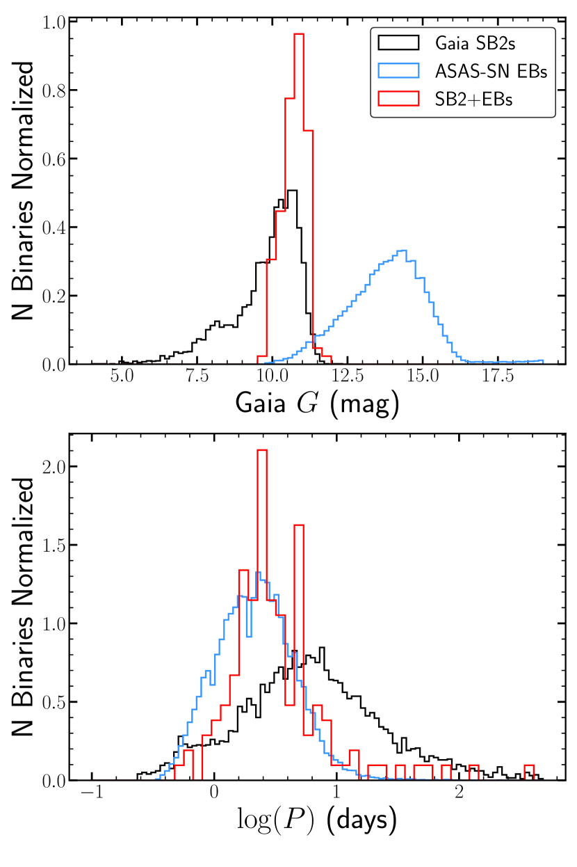
Figure 1: Top: normalized distributions of Gaia apparent $G$-band magnitudes for Gaia SB2s, ASAS-SN eclipsing binaries, and the crossmatched systems. Bottom: distribution of orbital periods. The Gaia spectroscopic binaries extend to longer orbital periods since the detectability of eclipsing binaries drops off as $P^{-2/3}$.

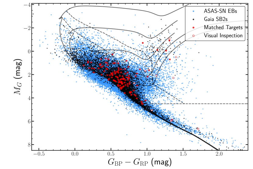
Figure 2: The extinction-corrected Gaia DR3 color-magnitude diagram (CMD). The ASAS-SN detached eclipsing binaries from R22 are shown in blue, the 5,376 Gaia SB2s are shown in black, and the eclipsing spectroscopic binaries are shown in red. The solid lines show MIST isochrones for ages of $10^{8}$ to $10^{10}$ years in intervals of $0.5$ dex. The flux of the isochrones are doubled in each band to represent binary stars of equal mass. The dashed lines show the boundaries of the giant and subgiant branches defined by R22. We note that one binary in the visual inspection group, CM Dra (Gaia DR3 1431176943768690816) is at $M_{G}\sim 10.6$ mag, below the range of this figure.

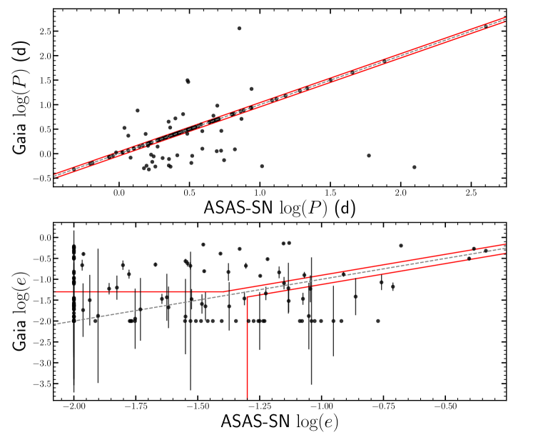
Figure 3: Comparison of periods and eccentricities from the Gaia SB2 orbits and ASAS-SN eclipsing binary light curves. The gray lines show the expected equality between the ASAS-SN and Gaia values. The region in between the red lines shows where we define the periods and eccentricities to be consistent. Eccentricities $\log e<-2$ are shown as $\log e=-2$ for this figure.

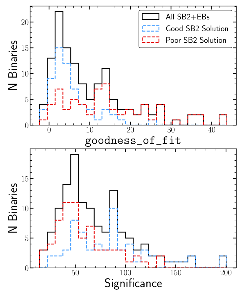
Figure 4: Distributions of the Gaia goodness_of_fit (top) and significance (bottom) for the full SB2+EB sample. We identify good orbital fits by comparing the Gaia and ASAS-SN periods and eccentricities (Figure 3).

Gaia DR3 includes a total of 5,376 systems with SB2 orbit solutions in the nss_two_body_orbit table. The majority of the targets are fairly bright, with apparent $G$ magnitudes ranging from 3.6 mag to 12.2 mag and a median of 10.1 mag. 1,053 of the Gaia SB2s are labeled as photometrically variable in Gaia DR3 and 533 are included in the vari_eclipsing_binary table. The optimal magnitude range for ASAS-SN targets is $11<V<17$ mag and $12<g<18$ mag. Figure 1 shows the distribution of apparent $G$ magnitude for the Gaia SB2 catalog and the Value-Added EB catalog.

We start by performing a positional cross-match with a search radius of $5\arcsec$ and identify 128 targets in common between the SB2 and EB catalogs. Figure 1 shows that these targets are found in the bright tail of the ASAS-SN catalog and the faint end of the SB2 catalog. The bottom panel of Figure 1 shows that the majority of systems identified in the cross-match have orbital periods $P<10$ days, although there are a handful of long-period systems included in both catalogs. The orbital period of the 128 targets ranges from 0.62 to 124.9 days with a median value of 2.68 days.

We use distances from Bailer-Jones et al. (2021), which include color and magnitude priors as part of the distance estimate, and extinction estimates from the mwdust (Bovy et al., 2016) 3-dimensional ‘Combined19’ dust map (Drimmel et al., 2003; Marshall et al., 2006; Green et al., 2019) to determine the extinction-corrected absolute magnitude and color. We use the MESA Isochrones & Stellar Tracks (MIST, Choi et al., 2016; Dotter, 2016) and follow the procedure described in R22 to divide the CMD into systems with main sequence, subgiant, and giant primaries. To remove systems with poor parallax or extinction estimates, we only report the evolutionary state for systems where the parallax divided by its standard error is $\texttt{parallax\_over\_error}>10$ and $A_{V}<2.0$ mag. Figure 2 shows the distribution of the SB2 catalog, the EB catalog, and the crossmatch between them on the CMD. For stars with $M_{G}\lesssim 4$ mag, there are fewer SB2s than ASAS-SN EBs below the binary main sequence since systems of nearly equal mass are more easily characterized in SB2 analysis.

The majority of the SB2+EB binaries are on the main sequence, although 18 and 5 are found on the subgiant and giant branch, respectively. We used ASAS-SN Sky Patrol v2 (Hart et al., in preparation) to visually inspect the $g$-band light curves of all 5,376 systems in the Gaia SB2 catalog folded at the Gaia orbital period. In total, we identify 200 additional eclipsing binaries. To expand our sample to stars of a wider range of mass and evolutionary state, we focus on either end of the main sequence ($M_{G}<1$ mag or $M_{G}>5$ mag) and stars that are subgiants/giants based on the CMD position and MIST isochrones. Figure 2 shows the 11 targets we added to our EB+SB2 catalog to expand our coverage of the CMD. While we add additional low-mass main sequence and giant/subgiant binaries, we find no additional high-mass main sequence binaries that are unsaturated ($V>11$ mag).

Although we expect the Gaia orbital period to be correct for these 11 systems since we identified the eclipses in the phase-folded light curve, we start by running the astrobase implementation of Box Least Squares (BLS) periodogram (Bhatti et al., 2018; Kovács et al., 2002) to determine a more precise period. We use a narrow period search window of $\pm 20\%$ of the Gaia orbital period. We manually clip outlying points due to saturation effects in the light curves. We then follow the procedure described in R22 to estimate the orbital inclination, eccentricity, argument of periastron, the ratio of effective temperatures, and the sum of the fractional radii with PHOEBE (Prša & Zwitter, 2005; Prša et al., 2016; Conroy et al., 2020). To summarize the procedure, we start by combining the results from the PHOEBE geometry estimator (Mowlavi et al., 2017) and the “eclipsing binaries via artificial intelligence” (EBAI) estimator (Prša et al., 2008) as initial estimations for the Nelder-Mead optimizer (Gao & Han, 2012). The resulting model will be used to set the initial conditions for the Markov Chain Monte Carlo (MCMC) fits.

Before we adopt values of the velocity semi-amplitudes from the Gaia SB2 solutions, we compare the ASAS-SN and Gaia periods and eccentricities to identify and remove poor SB2 orbital solutions. Figure 3 shows the ASAS-SN and Gaia orbital periods and eccentricities. We consider the SB2 solution to be reliable if the Gaia orbital period is within 10% of the ASAS-SN orbital period. We also require the Gaia eccentricity to be within 25% of the ASAS-SN eccentricity, or both eccentricities to be $e<0.05$. In total, only 70 SB2+EB systems meet these quality cuts. 18 of the systems with discrepant Gaia periods are relatively faint ($G\gtrsim 11$ mag), which could suggest lower-quality Gaia SB2 orbital fits in the tail of the magnitude distribution. This magnitude dependence is less clear for the comparison of eccentricities, but some of the systems where the ASAS-SN light curve suggests a near-circular orbit ($e\lesssim 0.01$) and Gaia prefers an eccentric orbit are also faint.

Jayasinghe et al. (2022) found similar disagreements in period and eccentricity when comparing the Gaia SB1s to the Ninth Catalog of Spectroscopic Orbits (SB9, Pourbaix et al., 2004) and Bashi et al. (2022) used LAMOST and GALAH radial velocities to consider which SB1s may have incorrect orbital parameters. Both found that many of the short-period Gaia SB1s have erroneously high eccentricities.

Figure 4 shows the distribution of the Gaia goodness_of_fit and significance parameters. The goodness_of_fit reports the “Gaussianized Chi-Square” statistic and is expected to have a median of zero and standard deviation of one, although we note that the median value for the full SB2 sample is 10.92. The top panel of Figure 4 shows that the SB2s with periods and eccentricities matching the ASAS-SN light curve solution generally have lower goodness_of_fit values, but there are some poor SB2 solutions with ${\tt goodness\_of\_fit}{}<5$. The significance parameter is defined as $K_{1}/\sigma_{K_{1}}$. While this statistic is generally useful for rejecting poor (Significance $\lesssim 20$) solutions (e.g., Jayasinghe et al., 2022), there does not seem to be a clear value here where Gaia SB2 orbital solutions can be rejected in the absence of constraints from the light curve. Bashi et al. (2022) combined the SB1 period, semi-amplitude, number of observations, goodness of fit, RV amplitude, and RV signal-to-noise ratio parameters to construct a “Score” statistic, but some of these parameters are not available for the Gaia SB2 sources. Since Gaia DR3 only provides the spectroscopic orbital solutions and not the individual radial velocities, it is clearly important to be cautious when interpreting the ensemble statistics in the Gaia nss_two_body_orbit SB2 tables given that only 50% of our eclipsing SB2s have reliable Gaia periods and eccentricities.

3 Eclipsing Binary Model Fitting

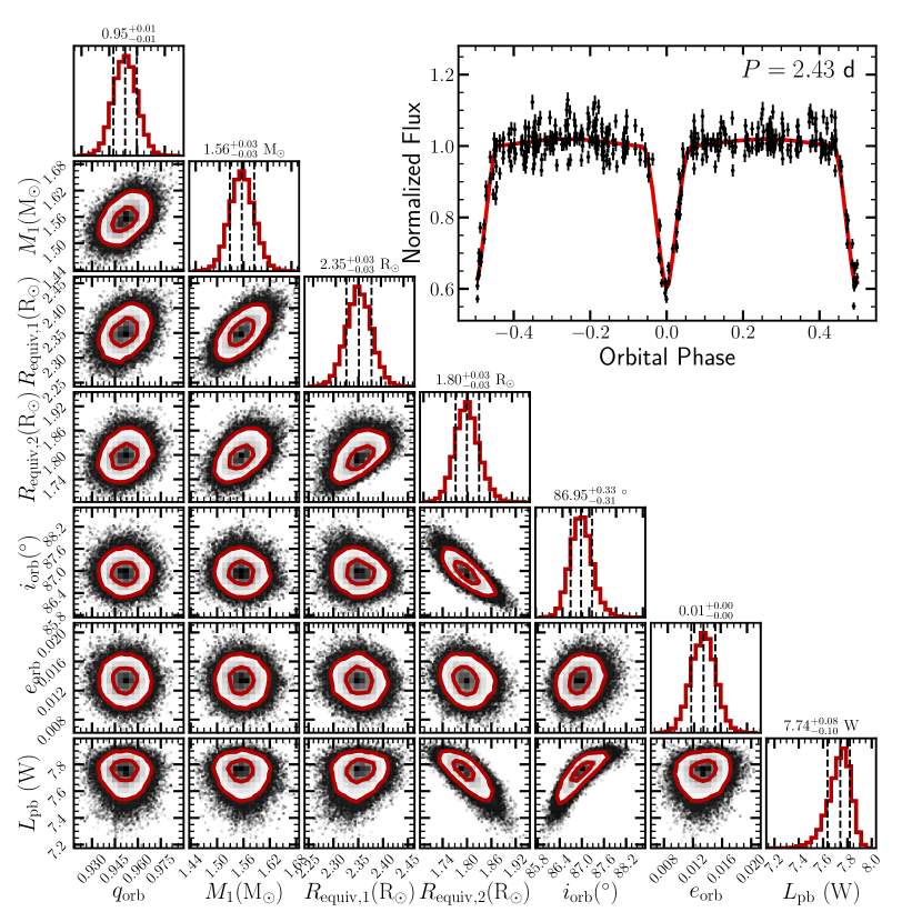
Figure 5: MCMC corner plot and light curve fit for Gaia DR3 154197232963101568.

For the 70 systems where the period and eccentricity of the Gaia SB2 solution are consistent with the results of the eclipsing binary model fit, we use either the ASAS-SN $V$- or $g$-band light curve, and select the light curve that is less affected by saturation. We change the passband luminosity mode to component--coupled, which uses the physical passband luminosity, $L_{\rm{pb}}$ for one star rather than a scaling based on the normalized fluxes. We run 200 iterations of Nelder-Mead optimization with $L_{\rm{pb}}$, the effective temperature ratio $T_{\rm{eff},2}/T_{\rm{eff},1}$, and the fractional radii $R_{1}/a$ and $R_{2}/a$, as free parameters.

We then set the mass ratio to be $q=K_{1}/K_{2}$, where $K_{1}$ and $K_{2}$ are the Gaia RV semi-amplitudes. We also set the value of the projected semi-major axis of the secondary to

$$a_{2}\sin(i)=K_{2}\left(\frac{P}{2\pi}\right)\sqrt{1-e^{2}}.$$ (1)

We use emcee (Foreman-Mackey et al., 2013) within PHOEBE to perform an MCMC fit on the ASAS-SN light curve. We set Gaussian priors on $q$ and $a_{2}\sin(i)$ using the Gaia DR3 values and errors on $K_{1}$ and $K_{2}$. The orbital period is fixed at the value from the BLS periodogram of the ASAS-SN light curve.

We sample over the mass ratio, $q$, the primary mass, $M_{1}$, the radii $R_{1}$ and $R_{2}$, the inclination $i$, the eccentricity, $e$, and the passband luminosity $L_{\rm{pb}}$. We use 5000 iterations with a 1000 iteration burn-in and 35 walkers. For some targets where the walkers have not yet converged by 1000 iterations, we run an additional 2000 iterations, increasing the burn-in accordingly. In some cases a few ($\lesssim 5$) of the walkers fail to converge. We manually set cutoffs in the log-probability of the walkers for these systems before adopting the final posterior distributions. Figure 5 shows an example of the MCMC posteriors and light curve fit for Gaia DR3 154197232963101568.

We calculate the Roche-lobe filling fraction, $f=R/R_{\rm{roche}}$, where $R_{\rm{roche}}$ can be estimated from the approximation (Eggleton, 1983),

$$R_{\rm{roche}}/a=\frac{0.49q^{2/3}}{0.6q^{2/3}+\ln{\left(1+q^{1/3}\right)}}.$$ (2)

The filling fraction can be used to evaluate the degree to which systems are detached and can be thought of as evolving independently, without mass transfer.

4 Results

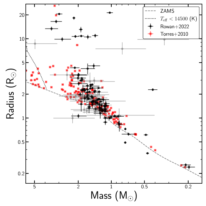
Figure 6: Masses and radii of eclipsing SB2s derived from ASAS-SN eclipsing binary light curves and Gaia SB2 orbital solutions. The gray points shows stars with fractional mass error $>20\%$. The Torres et al. (2010) catalog stars are shown in red. The gray dashed line shows the MIST single-star ZAMS isochrone and the gray dotted line shows the cutoff at $T_{\rm{eff}}<14500$ K for the Gaia RVS measurements.

Table 1: Stellar parameters from the MCMC fits to the ASAS-SN light curves with constraints from Gaia spectroscopic orbits. The Roche-lobe filling fractions of the primary and secondary are $f_{1}$ and $f_{2}$, respectively. The evolutionary state is based on the CMD position in Figure 2. The full table is available online at https://asas-sn.osu.edu/binaries/mass-radius and in the electronic version of the paper.

Gaia DR3 Source	Period	Mass Ratio	$M_{1}$	$M_{2}$	$R_{1}$	$R_{1}$	$f_{1}$	$f_{1}$	$e$	$i$	State
	(d)		(M⊙)	(M⊙)	(R⊙)	(R⊙)				(∘)
40041022325608704	$2.808646$	$0.99^{+0.03}_{-0.03}$	$1.28^{+0.11}_{-0.10}$	$1.27^{+0.13}_{-0.12}$	$1.47^{+0.11}_{-0.15}$	$1.30^{+0.15}_{-0.15}$	$0.338415$	$0.300173$	$0.01^{+0.01}_{-0.01}$	$85.76^{+0.37}_{-0.21}$	MS
154197232963101568	$2.431772$	$0.95^{+0.01}_{-0.01}$	$1.56^{+0.03}_{-0.03}$	$1.48^{+0.04}_{-0.04}$	$2.35^{+0.03}_{-0.03}$	$1.80^{+0.03}_{-0.03}$	$0.556776$	$0.435488$	$0.01^{+0.00}_{-0.00}$	$86.95^{+0.33}_{-0.31}$	SG
428267308105062528	$3.289680$	$0.95^{+0.21}_{-0.10}$	$1.89^{+0.85}_{-0.63}$	$1.83^{+0.60}_{-0.56}$	$1.95^{+0.27}_{-0.33}$	$1.96^{+0.43}_{-0.33}$	$0.354284$	$0.361245$	$0.01^{+0.00}_{-0.00}$	$83.98^{+0.44}_{-0.33}$	MS
453147263375440384	$4.586150$	$0.98^{+0.02}_{-0.02}$	$1.84^{+0.10}_{-0.09}$	$1.81^{+0.12}_{-0.10}$	$3.03^{+0.10}_{-0.24}$	$2.28^{+0.35}_{-0.24}$	$0.445720$	$0.336974$	$0.00^{+0.00}_{-0.00}$	$84.31^{+0.79}_{-0.55}$	MS
533425940213217920	$4.860321$	$0.97^{+0.02}_{-0.02}$	$1.54^{+0.06}_{-0.06}$	$1.48^{+0.08}_{-0.07}$	$2.63^{+0.07}_{-0.07}$	$2.39^{+0.08}_{-0.07}$	$0.394413$	$0.363752$	$0.00^{+0.00}_{-0.00}$	$87.43^{+0.16}_{-0.13}$	SG
535419732749344000	$2.948269$	$0.87^{+0.32}_{-0.03}$	$2.44^{+0.43}_{-0.37}$	$2.13^{+0.33}_{-0.31}$	$1.91^{+0.12}_{-0.10}$	$4.33^{+0.22}_{-0.22}$	$0.340413$	$0.821817$	$0.00^{+0.00}_{-0.00}$	$87.73^{+1.59}_{-2.20}$	SG
555108687465591040	$6.334426$	$0.95^{+0.14}_{-0.04}$	$1.00^{+0.17}_{-0.14}$	$0.96^{+0.14}_{-0.12}$	$0.91^{+0.11}_{-0.09}$	$0.95^{+0.08}_{-0.10}$	$0.131480$	$0.139853$	$0.06^{+0.00}_{-0.00}$	$88.67^{+0.29}_{-0.15}$	MS
583022706417479296	$12.185384$	$0.96^{+0.01}_{-0.01}$	$1.20^{+0.03}_{-0.03}$	$1.15^{+0.04}_{-0.04}$	$3.93^{+0.52}_{-0.52}$	$3.93^{+0.73}_{-1.27}$	$0.347034$	$0.353851$	$0.01^{+0.01}_{-0.01}$	$83.30^{+4.82}_{-1.34}$	SG
681609355666984192	$2.703459$	$0.96^{+0.14}_{-0.05}$	$1.54^{+0.29}_{-0.26}$	$1.48^{+0.23}_{-0.23}$	$2.52^{+0.17}_{-0.18}$	$1.47^{+0.21}_{-0.16}$	$0.559009$	$0.332373$	$0.00^{+0.00}_{-0.00}$	$79.89^{+0.94}_{-0.94}$	MS
690638579515175552	$2.380733$	$0.96^{+0.01}_{-0.01}$	$1.18^{+0.03}_{-0.03}$	$1.13^{+0.04}_{-0.03}$	$1.62^{+0.21}_{-0.22}$	$1.67^{+0.14}_{-0.24}$	$0.428208$	$0.447758$	$0.00^{+0.00}_{-0.00}$	$85.24^{+0.75}_{-0.38}$	MS
690885522954174080	$0.647598$	$0.81^{+0.04}_{-0.04}$	$0.87^{+0.10}_{-0.10}$	$0.70^{+0.11}_{-0.10}$	$1.05^{+0.04}_{-0.04}$	$0.63^{+0.03}_{-0.03}$	$0.721960$	$0.474742$	$0.11^{+0.01}_{-0.01}$	$84.77^{+0.36}_{-0.62}$	MS
947509303493752832	$3.481821$	$0.99^{+0.05}_{-0.05}$	$1.23^{+0.20}_{-0.17}$	$1.22^{+0.23}_{-0.20}$	$1.31^{+0.10}_{-0.09}$	$1.23^{+0.09}_{-0.09}$	$0.263934$	$0.248808$	$0.00^{+0.00}_{-0.00}$	$88.55^{+0.19}_{-0.15}$	MS
1204875013864088576	$3.288118$	$0.97^{+0.12}_{-0.14}$	$1.64^{+0.72}_{-0.59}$	$1.56^{+0.86}_{-0.63}$	$1.97^{+0.38}_{-0.36}$	$2.89^{+0.85}_{-1.24}$	$0.375038$	$0.561835$	$0.01^{+0.01}_{-0.01}$	$72.44^{+4.40}_{-2.17}$	MS
1272930282497618048	$5.117104$	$0.95^{+0.07}_{-0.08}$	$1.43^{+0.40}_{-0.26}$	$1.34^{+0.44}_{-0.26}$	$2.98^{+0.29}_{-0.30}$	$2.11^{+0.36}_{-0.20}$	$0.440978$	$0.322579$	$0.00^{+0.00}_{-0.00}$	$88.73^{+0.85}_{-3.41}$	SG
1387290280744129152	$0.846993$	$0.76^{+0.62}_{-0.04}$	$1.77^{+0.58}_{-0.49}$	$1.36^{+0.40}_{-0.37}$	$1.28^{+0.12}_{-0.13}$	$1.46^{+0.14}_{-0.15}$	$0.577313$	$0.741876$	$0.00^{+0.00}_{-0.00}$	$87.25^{+0.26}_{-0.21}$	MS

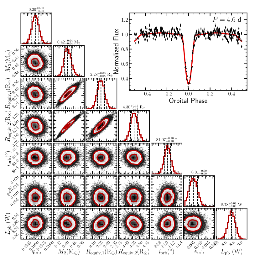
Figure 7: MCMC forner plot and light curve fit for Gaia DR3 1762094209603752192. This binary has one star with $M<1$ M_⊙ and $R>2$ $R_{\odot}$ and one on the subgiant branch, which could suggest a history of mass transfer.

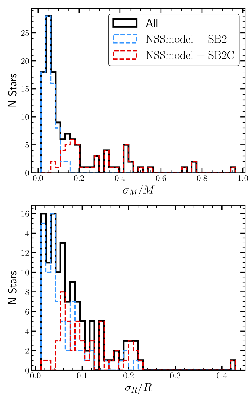
Figure 8: Fractional error on the masses (top) and radii (bottom) from the MCMC fits to the ASAS-SN light curves with orbital constraints from Gaia SB2s. The binaries with the circular orbital solution (NSSmodel=SB2C) make up the majority of the high fractional error tails in mass and radius.

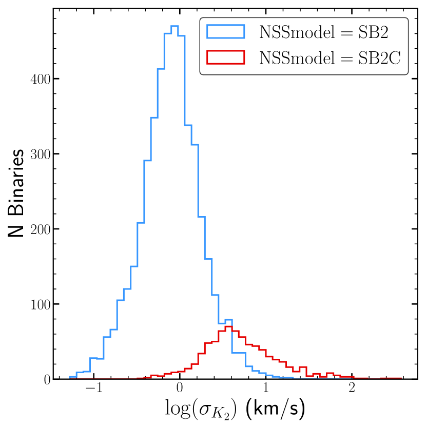
Figure 9: Distribution of the error on the velocity semi-amplitude of the secondary, $\sigma_{K_{2}}$ for the full sample of Gaia SB2s colored by the type of model used. The Gaia SB2s with the circular orbit model generally have larger errors on $K_{2}$.

Table 1 reports the Gaia Source information, MCMC posteriors, and the evolutionary state of the primary based its the CMD position. All of the light curves and corner plots are available online at https://asas-sn.osu.edu/binaries/mass-radius, and in the electronic version of the paper.

Figure 6 shows the masses and radii of our sample. The gray dashed line shows the single star Solar metallicity zero-age main sequence (ZAMS) from the MESA Isochrones & Stellar Tracks (MIST, Choi et al., 2016; Dotter, 2016). Figure 6 also compares our sample to the masses and radii in Torres et al. (2010). The Torres et al. (2010) catalog includes the selection criteria that both components have masses and radii errors $<3\%$, so it is not surprising that our uncertainties on the stellar parameters are larger, but we find results consistent with expectations for main-sequence stars. We report masses and radii of 12 stars on the giant branch, a sparsely populated region in the Torres et al. (2010) catalog. Our catalog also has fewer high-mass main sequence stars. This is primarily due to the saturation limit of ASAS-SN, but Gaia RVS data also uses the limit $T_{\rm{eff}}<14500$ K, which is shown by the gray dotted line in Figure 6 for Solar-metallicity evolutionary tracks. We did identify $\sim 10$ eclipsing binaries on the upper main sequence during visual inspection, but all were saturated in the ASAS-SN light curves. The lowest mass system in our catalog, CM Draconis, was also included in the Torres et al. (2010) catalog, and our results are consistent within $1\sigma$.

Some of our stars have masses and radii that place them below the ZAMS line. The deviation from the Solar metallicity ZAMS is too large to be a metallicity effect, so these stars probably have poor Gaia SB2 solutions or histories of mass transfer. Some of these systems are at shorter orbital periods, but none have especially high Roche-lobe filling fractions, suggesting mass-transfer may not be the source of the deviation. These systems also do not have large goodness_of_fit values.

There are also three stars with $M<1$ M_⊙ and $R>2$ $R_{\odot}$. Two of these are in the same binary, Gaia DR3 5339144356205089408. This system has Roche-lobe filling fractions of $f_{1}=0.48$ and $f_{2}=0.94$ for the primary and secondary, respectively, which may indicate a history of mass-transfer. The third star with low mass and large radius is Gaia DR3 1762094209603752192. The other star in this binary is on the subgiant branch, with $M_{1}=2.15$ M_⊙ and $R_{1}=4.3$ R_⊙. There is also a large difference in eclipse depth (see Figure 7), suggesting that the more luminous star is also hotter. Both stars have Roche-lobe filling factors $0.5<f<0.6$, which could suggest that if mass transfer did occur, it is not currently ongoing.

Figure 8 shows the distribution of the mass and radius uncertainties. For systems with asymmetric posteriors, we report the larger of the $\pm 1\sigma$ uncertainties. The median uncertainty on the mass is 7.9%, and the median uncertainty on the radius is 6.3%. Gaia DR3 includes two solution types for SB2s: a standard double-lined binary where the eccentricity is a free parameter ($\rm{NSSmodel}=\rm{SB2}$) and a simplified, circular model ($\rm{NSSmodel}=\rm{SB2C}$). Figure 8 shows that the binaries with the circular orbit model correspond to almost all of the systems with high fractional errors on the mass and the radius.

The SB2s with the circular orbit model also generally have higher errors on the velocity semi-amplitude of the secondary, $\sigma_{K_{2}}$ (Figure 9). Since the velocity semi-amplitudes are used in our PHOEBE models to set the mass ratio, projected semi-major axis, and the priors for the MCMC runs, a large $\sigma_{K_{2}}$ will produce a large $\sigma_{M}/M$. If we only consider binaries with $\rm{NSSmodel}=\rm{SB2}$, the median uncertainty on the mass is 4.8% and the median uncertainty on the radius is 6.3%.

5 Summary

Gaia Data Release 3 includes spectroscopic orbits for more than 181,000 single-lined spectroscopic binaries and 5,376 double-lined spectroscopic binaries. We cross-match the catalog of SB2s with our ASAS-SN eclipsing binary catalog and further extend the sample through visual inspection. We compare the period and eccentricity from the ASAS-SN light curve to the Gaia values (Figure 3) and find that only 50% of systems have Gaia orbits in agreement with the light curve fits. Although it is difficult to identify the source of the discrepancy in the Gaia solution without the individual RVs, we do see more disagreement at shorter periods and at fainter apparent magnitudes. For the single-lined binaries, Bashi et al. (2022) combined various Gaia radial velocity statistics to reject poor Gaia orbits and identified a sample of $\sim 90,000$ of the $\sim 181,000$ as having good SB1 orbits, but no such metrics currently exist for SB2s.

For the 70 systems where the Gaia solution is consistent with the eclipsing binary light curve, we use PHOEBE to fit the light curve constrained by the velocity semi-amplitudes to derive masses and radii for 122 stars. Of these 122 stars, 61 have fractional mass and radius uncertainties less than 10% (Figure 8). We find that many of the systems with high fractional mass errors use the Gaia circular orbit model “SB2C”, which tend to have larger uncertainties on $K_{2}$ (Figure 9). The uncertainties in our catalog are larger than those in the Torres et al. (2010) sample of eclipsing SB2s (Figure 6), but we only use publicly available data from large surveys.

Our sample is strongly limited by the differences between the magnitude range of ASAS-SN and the Gaia Radial Velocity Spectrometer. Since almost all of the Gaia SB2s are bright ($G<12$ mag), and ASAS-SN light curves start to saturate at $G\sim 11$, only a fraction of the eclipsing spectroscopic binaries observed by Gaia have been modeled here. Large photometric surveys of brighter stars, such as ASAS (Pojmanski, 2002; Paczyński et al., 2006) and the Kilodegree Extremely Little Telescope (KELT, Pepper et al., 2007) could be used to identify and characterize these brighter systems. The Gaia light curves often have too few epochs for modeling detached eclipsing binary light curves, but future releases will provide additional $G$, $G_{\rm{BP}}$, and $G_{\rm{RP}}$ observations for millions of binaries. Multi-band light curves could also be used to constrain absolute temperatures of the stars, providing additional constraints on relations between stellar parameters.

In total, we report masses and radii for 12 giants. One of these systems, Gaia DR3 509431332327692032, has the longest period, $P=401.7$ d, and the highest eccentricity, $e=0.46$, of the binaries in our sample. Since masses of giants are difficult to determine through isochrone fitting, these systems are valuable for expanding the small sample size of giants with precise physical parameters. Long time period photometry is crucial to detecting and characterizing these systems. Our ASAS-SN eclipsing binary catalog contains more than 600 eclipsing binaries on the giant branch that could be used to expand the population of giants with dynamical masses and radii.

The sample of spectroscopic binaries will continue to expand with future Gaia data releases and and upcoming spectroscopic surveys such as Milky Way Mapper (Kollmeier et al., 2017). Large catalogs of eclipsing binaries can be used not only to identify eclipsing SB2s, but also to provide initial conditions for detailed modeling of the light curve and radial velocity data.

Data Availability

The ASAS-SN photometric data underlying this article are available in the ASAS-SN eclipsing binaries database (https://asas-sn.osu.edu/binaries/mass-radius) and the ASAS-SN Photometry Database (https://asas-sn.osu.edu/photometry). The data underlying this article are available in the article and in its online supplementary material.

References

- Andersen (1991) Andersen J., 1991, A&ARv, 3, 91
- Bailer-Jones et al. (2021) Bailer-Jones C. A. L., Rybizki J., Fouesneau M., Demleitner M., Andrae R., 2021, VizieR Online Data Catalog, p. I/352
- Bashi et al. (2022) Bashi D., Shahaf S., Mazeh T., Faigler S., Dong S., El-Badry K., Rix H.-W., Jorissen A., 2022, arXiv e-prints, p. arXiv:2207.08832
- Beck et al. (2014) Beck P. G., et al., 2014, A&A, 564, A36
- Beck et al. (2022) Beck P. G., et al., 2022, arXiv e-prints, p. arXiv:2202.02373
- Benbakoura et al. (2021) Benbakoura M., et al., 2021, A&A, 648, A113
- Bhatti et al. (2018) Bhatti W., lgbouma Joshua 2018, Waqasbhatti/Astrobase: Astrobase V0.3.8, doi:10.5281/zenodo.1185231
- Bódi & Hajdu (2021) Bódi A., Hajdu T., 2021, ApJS, 255, 1
- Bovy et al. (2016) Bovy J., Rix H.-W., Green G. M., Schlafly E. F., Finkbeiner D. P., 2016, ApJ, 818, 130
- Brogaard et al. (2018) Brogaard K., et al., 2018, MNRAS, 476, 3729
- Choi et al. (2016) Choi J., Dotter A., Conroy C., Cantiello M., Paxton B., Johnson B. D., 2016, ApJ, 823, 102
- Conroy et al. (2020) Conroy K. E., et al., 2020, ApJS, 250, 34
- Cui et al. (2012) Cui X.-Q., et al., 2012, Research in Astronomy and Astrophysics, 12, 1197
- Dotter (2016) Dotter A., 2016, ApJS, 222, 8
- Drimmel et al. (2003) Drimmel R., Cabrera-Lavers A., López-Corredoira M., 2003, A&A, 409, 205
- Duck et al. (2022) Duck A., Gaudi B. S., Eastman J. D., Rodriguez J. E., 2022, arXiv e-prints, p. arXiv:2209.09266
- Eastman et al. (2013) Eastman J., Gaudi B. S., Agol E., 2013, PASP, 125, 83
- Eggleton (1983) Eggleton P. P., 1983, ApJ, 268, 368
- Enoch et al. (2010) Enoch B., Collier Cameron A., Parley N. R., Hebb L., 2010, A&A, 516, A33
- Foreman-Mackey et al. (2013) Foreman-Mackey D., Hogg D. W., Lang D., Goodman J., 2013, PASP, 125, 306
- Frandsen et al. (2013) Frandsen S., et al., 2013, A&A, 556, A138
- Gaia Collaboration et al. (2022) Gaia Collaboration et al., 2022, arXiv e-prints, p. arXiv:2208.00211
- Gao & Han (2012) Gao F., Han L., 2012, Optim Appl, 51, 259
- Gaulme et al. (2013) Gaulme P., McKeever J., Rawls M. L., Jackiewicz J., Mosser B., Guzik J. A., 2013, ApJ, 767, 82
- Gaulme et al. (2014) Gaulme P., Jackiewicz J., Appourchaux T., Mosser B., 2014, ApJ, 785, 5
- Gaulme et al. (2016) Gaulme P., et al., 2016, ApJ, 832, 121
- Graczyk et al. (2011) Graczyk D., et al., 2011, Acta Astron., 61, 103
- Green et al. (2019) Green G. M., Schlafly E., Zucker C., Speagle J. S., Finkbeiner D., 2019, ApJ, 887, 93
- Hambleton et al. (2022) Hambleton K., Prša A., Fleming S. W., Mahadevan S., Bender C. F., 2022, ApJ, 931, 75
- Hekker et al. (2010) Hekker S., et al., 2010, ApJ, 713, L187
- Hełminiak et al. (2021) Hełminiak K. G., et al., 2021, MNRAS, 508, 5687
- Huang et al. (2020a) Huang C. X., et al., 2020a, Research Notes of the American Astronomical Society, 4, 204
- Huang et al. (2020b) Huang C. X., et al., 2020b, Research Notes of the American Astronomical Society, 4, 206
- Jayasinghe et al. (2019) Jayasinghe T., et al., 2019, MNRAS, 486, 1907
- Jayasinghe et al. (2022) Jayasinghe T., Rowan D. M., Thompson T. A., Kochanek C. S., Stanek K. Z., 2022, arXiv e-prints, p. arXiv:2207.05086
- Kirk et al. (2016) Kirk B., et al., 2016, AJ, 151, 68
- Kjeldsen & Bedding (1995) Kjeldsen H., Bedding T. R., 1995, A&A, 293, 87
- Kochanek et al. (2017) Kochanek C. S., et al., 2017, PASP, 129, 104502
- Kollmeier et al. (2017) Kollmeier J. A., et al., 2017, arXiv e-prints, p. arXiv:1711.03234
- Kounkel et al. (2021) Kounkel M., et al., 2021, AJ, 162, 184
- Kovács et al. (2002) Kovács G., Zucker S., Mazeh T., 2002, A&A, 391, 369
- Kunimoto et al. (2021) Kunimoto M., et al., 2021, Research Notes of the American Astronomical Society, 5, 234
- Majewski et al. (2017) Majewski S. R., et al., 2017, AJ, 154, 94
- Marshall et al. (2006) Marshall D. J., Robin A. C., Reylé C., Schultheis M., Picaud S., 2006, A&A, 453, 635
- Mowlavi et al. (2017) Mowlavi N., et al., 2017, A&A, 606, A92
- Paczyński et al. (2006) Paczyński B., Szczygieł D. M., Pilecki B., Pojmański G., 2006, MNRAS, 368, 1311
- Pawlak et al. (2013) Pawlak M., et al., 2013, Acta Astron., 63, 323
- Pepper et al. (2007) Pepper J., et al., 2007, PASP, 119, 923
- Petrosky et al. (2021) Petrosky E., Hwang H.-C., Zakamska N. L., Chandra V., Hill M. J., 2021, MNRAS, 503, 3975
- Pietrukowicz et al. (2013) Pietrukowicz P., et al., 2013, Acta Astron., 63, 115
- Pojmanski (2002) Pojmanski G., 2002, Acta Astron., 52, 397
- Pourbaix et al. (2004) Pourbaix D., et al., 2004, A&A, 424, 727
- Prša & Zwitter (2005) Prša A., Zwitter T., 2005, ApJ, 628, 426
- Prša et al. (2008) Prša A., Guinan E. F., Devinney E. J., DeGeorge M., Bradstreet D. H., Giammarco J. M., Alcock C. R., Engle S. G., 2008, ApJ, 687, 542
- Prša et al. (2011) Prša A., et al., 2011, AJ, 141, 83
- Prša et al. (2016) Prša A., et al., 2016, ApJS, 227, 29
- Prša et al. (2022) Prša A., et al., 2022, ApJS, 258, 16
- Qian et al. (2017) Qian S.-B., He J.-J., Zhang J., Zhu L.-Y., Shi X.-D., Zhao E.-G., Zhou X., 2017, Research in Astronomy and Astrophysics, 17, 087
- Qian et al. (2018) Qian S. B., Zhang J., He J. J., Zhu L. Y., Zhao E. G., Shi X. D., Zhou X., Han Z. T., 2018, ApJS, 235, 5
- Ratajczak et al. (2021) Ratajczak M., et al., 2021, MNRAS, 500, 4972
- Ricker et al. (2015) Ricker G. R., et al., 2015, Journal of Astronomical Telescopes, Instruments, and Systems, 1, 014003
- Rodríguez Martínez et al. (2022) Rodríguez Martínez R., et al., 2022, arXiv e-prints, p. arXiv:2208.07883
- Rowan et al. (2022a) Rowan D. M., et al., 2022a, arXiv e-prints, p. arXiv:2210.06486
- Rowan et al. (2022b) Rowan D. M., et al., 2022b, MNRAS, 517, 2190
- Shappee et al. (2014) Shappee B. J., et al., 2014, ApJ, 788, 48
- Slawson et al. (2011) Slawson R. W., et al., 2011, AJ, 142, 160
- Soszyński et al. (2016) Soszyński I., et al., 2016, Acta Astron., 66, 405
- Steinmetz et al. (2006) Steinmetz M., et al., 2006, AJ, 132, 1645
- Themeßl et al. (2018) Themeßl N., et al., 2018, MNRAS, 478, 4669
- Torres et al. (2010) Torres G., Andersen J., Giménez A., 2010, A&ARv, 18, 67