SceneRF: Self-Supervised Monocular 3D Scene Reconstruction
with Radiance Fields

Abstract

3D reconstruction from a single 2D image was extensively covered in the literature but relies on depth supervision at training time, which limits its applicability. To relax the dependence to depth we propose SceneRF, a self-supervised monocular scene reconstruction method using only posed image sequences for training. Fueled by the recent progress in neural radiance fields (NeRF) we optimize a radiance field though with explicit depth optimization and a novel probabilistic sampling strategy to efficiently handle large scenes. At inference, a single input image suffices to hallucinate novel depth views which are fused together to obtain 3D scene reconstruction. Thorough experiments demonstrate that we outperform all baselines for novel depth views synthesis and scene reconstruction, on indoor BundleFusion and outdoor SemanticKITTI. Code is available at https://astra-vision.github.io/SceneRF .

1 Introduction

Humans evolve in a 3D physical world where even the slightest motion requires a thorough understanding of their surroundings to avoid collisions. While binocular vision is an evident evolutionary edge, physiological studies suggest that humans can sense depth even with monocular vision [31]. Despite a long-standing line of research [72, 84, 66] this is yet unequaled by computer vision algorithms, which mostly rely on multiple-views to reconstruct complex scenes [59]. However, estimating 3D from a single view would unveil novel applications in a world flooded with consumer cameras where mobile robots, like autonomous cars, still require costly depth sensors [6, 4].

A small portion of the 3D field addressed reconstruction of complex scenes from a single image [26, 85, 8, 12] but they all require depth supervision which discourage acquisition of image-only datasets. Meanwhile, Neural Radiance Field [45] (NeRF), which optimizes a radiance field self-supervisedly from one or more views, unraveled many descendants [78] with unprecedented performance on novel views synthesis. They are however, mostly limited to objects when it comes to single-view input [40, 51, 47]. For complex scenes, besides [34] all train on synthetic data [63] or require additional geometrical cues to train on real data [57, 14, 59]. Reducing the need of supervision on complex scenes would lower our dependency to costly-acquired datasets.

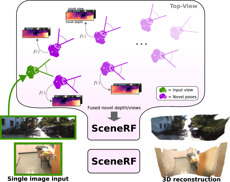
Figure 1: SceneRF overview. From a single input image, SceneRF synthesizes novel depth/views, at arbitrary poses, which are then fused to estimate 3D reconstruction. It relies on an image-conditioned NeRF (here, $f(\cdot)$) trained self-supervisedly on image sequences with pose.

In this work, we address single-view reconstruction of complex (and possibly large) scenes, in a fully self-supervised manner. SceneRF trains only with sequences of posed images to optimize a large neural radiance fields (NeRF). Fig. 1 illustrates inference where a single RGB image suffices to reconstruct the 3D scene from the fusion of synthesized novel depths/views, sampled at arbitrary locations. We build upon PixelNeRF [81] and propose specific design choices to explicitly optimize depth. Because large scenes hold their own challenges, we introduce a novel probabilistic ray sampling to efficiently choose the sparse locations to optimize within the large radiance volume, and introduce a Spherical U-Net, which aims is to enable hallucination beyond the input image field of view. We summarize our contributions below:

• We build on custom design choices to explicitly optimize depth (Sec. 3.1) with a Spherical U-Net (Sec. 3.3) – altogether allowing use of our radiance field for scene reconstruction (Sec. 3.4),

• Our probabilistic ray sampling (Sec. 3.2) learns to model the continuous density volume with a mixture of Gaussians – boosting both performance and efficiency,

• To the best of our knowledge, we propose the first self-supervised large scene reconstruction method using a single-view as input. Results on indoor and driving scenes show that SceneRF even outperforms depth-supervised baselines (Sec. 4).

2 Related work

As the 3D literature recently blossomed with the rise of NeRF methods [78], we limit our review to the smaller portion of works using a single input view, and study the literature along two axes related to our work: novel views/depths synthesis and 3D reconstruction.

Novel views/depths synthesis.

Rendering novel views from an image has been a long-lasting research problem [24, 70, 52, 79]. Although most recent works rely on generalizable NeRFs like PixelNerf [81], MINE [34], or GRF [71] which learn a representation generalizable to unseen input images. The almost entire single-view literature however focuses on objects which hold specific challenges such as shape and appearance disentanglement [30, 58], exploiting symmetry priors [36], or category-centric/agnostic view synthesis [56, 39]. In the latter, objects are usually on a plain background though CO3D [56] handle objects on cluttered scenes or large-scale scenes being synthetic as in SEE3D [63], or real as in MINE [34] or AutoRF [47]. Specific to complex scenes, [34] synthesizes novel depths and views building on Multiplane Images, while very recently [76] explored prediction of density fields trained with stereo or monocular sequences though getting limited improvement on the latter.

In general, depth supervision is shown to improve quality and convergence speed [14, 7, 57, 59], leveraging, for example, structure from motion [14, 59] or Lidar data [57]. Any NeRF-based method can implicitly optimize depth but those doing it explicitly still require depth supervision. Instead, we explicitly optimize depth self-supervisedly.
Since NeRF optimizes radiance field only at sparse locations, efficient sampling strategy is needed to avoid prohibitive cost [48]. Departing from the initial hierarchical sampling [45], a log warping strategy was proposed in DONeRF [48] with depth supervision, while [32] uses a pretrained NeRF, and [32] employs dual sampling-shading networks in a 4-stage training scheme. We inspire from above works but approximates the continuous density volume as a mixture of Gaussians from which we can efficiently sample, without any complex setup.

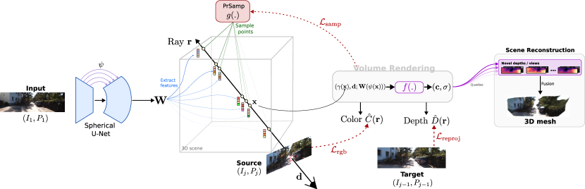
Figure 2: Scene Representation Learning in SceneRF. We leverage generalizable neural radiance field (NeRF) to generate novel depth views, conditioned on a single input frame. During training, for each ray $\mathbf{r}$ in addition to color $\hat{C}$, we explicitly optimize depth $\hat{D}$ with a reprojection loss $\mathcal{L}_{\text{reproj}}$ (Sec. 3.1), introduce a Probabilistic Ray Sampling strategy (PrSamp, Sec. 3.2) to sample points more efficiently. To hallucinate features outside the input FOV, we propose a spherical U-Net (Sec. 3.3). Finally, our scene reconstruction scheme (Sec. 3.4) fuses novel views/depths to estimate the 3D mesh.

3D reconstruction

While early deep methods focused on reconstruction with explicit representations:  like voxels [77], point clouds [1, 17, 80] or meshes [73, 10, 38], recently, implicit representations gain popularity [53, 54, 55, 28]. A common practice for 3D object reconstruction is to employ object detectors [29, 19, 86, 22]. A number of works addressed holistic 3D scene understanding, seeking prediction of geometry and semantics for indoor [50, 26, 85, 33, 67, 88, 12, 16] and outdoor scenes [82], or both [8]. When semantic and geometry are estimated jointly it is referred as semantic scene completion (SSC), recently surveyed in [61]. Relevant to this work, MonoScene [8] and its descendants [43, 37, 27] address SSC with single-input view but requiring 3D supervision.

A few alternatives exist for self-supervised 3D reconstruction. The straightforward use of monocular depth estimation, reviewed in [46], inherently limits reconstruction to the visible surface. Differentiable renderers are also popular, trained with views and poses [51, 65, 15]. To alleviate the need of color rendering, some optimize silhouettes [23] or 2D projection [89]. Despite dazzling visuals, they remain object-centric. Instead, we learn scene reconstruction self-supervisedly from a general radiance field.

3 SceneRF

SceneRF learns the implicit scene geometry from a single monocular RGB image, training in a self-supervised manner with image-conditioned Neural Radiance Fields (NeRFs) [45, 81]. Given a set $\mathcal{S}$ of image sequences with $m$ temporally consecutive RGB images with corresponding poses, denoted $\{(I^{s}_{1},P^{s}_{1}),\dots,(I^{s}_{m},P^{s}_{m})\}_{s\in\mathcal{S}}$, we learn a neural representation conditioned on the first frame of the sequence $\{I^{s}_{1}\}_{s\in\mathcal{S}}$. The conditioning learned is shared across sequences and self-supervisedly optimized with all other frames (i.e., $\{I^{s}_{2},...,I^{s}_{m}\}_{s\in\mathcal{S}}$). Subsequently, it can be used for 3D reconstruction from a single RGB image.

In Sec. 3.1 we elaborate on our usage of NeRF for novel depth synthesis relying on optimization with a reprojection loss. We then detail two major components. First, in Sec. 3.2 we introduce a topology-preserving strategy to efficiently sample points close to the surface. Second, to hallucinate the scene beyond the input image field of view, we introduce our custom U-Net Sec. 3.3 with a spherical decoder. Ultimately, the above design choices allow us to synthesize novel depth/views at arbitrary positions which are then fused into a single 3D reconstruction Sec. 3.4.

3.1 NeRF for novel depth synthesis

In their original formulation, NeRFs [45, 81] optimize a continuous volumetric radiance field $f(.)=(\sigma,\mathbf{c})$ such that for a given 3D point $\mathbf{x}\in\mathbb{R}^{3}$ and viewing direction $\mathbf{d}\in\mathbb{R}^{3}$, it returns a density $\sigma$ and RGB color $\mathbf{c}$. In the following, we build on PixelNeRF [81] to learn a generalizable radiance field across sequences, and introduce new design choices to efficiently synthesize novel depth views.

The training of SceneRF is illustrated in Fig. 2. Given the first input frame ($I_{1}$) of a sequence, we extract a feature volume $\mathbf{W}=\textit{E}(I_{1})$ with our SU-Net (Sec. 3.3). We then select randomly a source future frame $I_{j},2\leq j\leq m$, and randomly sample $\ell$ pixels from it. Given known source pose and camera intrinsics, we efficiently sample $N$ points along the rays passing through these pixels (Sec. 3.2). Each sampled point $\mathbf{x}$ is then projected on a sphere with $\psi(\cdot)$ so we can retrieve the corresponding input image feature vector $\mathbf{W}(\psi(\mathbf{x}))$ from bilinear interpolation. The latter is passed to the NeRF MLP $f(\cdot)$, along with viewing direction $\mathbf{d}$ and positional encoding $\gamma(\mathbf{x})$, to predict the point density $\sigma$ and RGB color $\mathbf{c}$ in the input frame coordinates. This writes:

$$f(\gamma(\mathbf{x}),\mathbf{d};\mathbf{W}(\psi(\mathbf{x})))=(\mathbf{c},\sigma)$$ (1)

As in original NeRF [45], quadrature approximates the color $\hat{C}(\mathbf{r})$ of camera ray $\mathbf{r}$ from colors sampled along the ray. For the sake of generality, we write it as:

$$\hat{C}(\mathbf{r})=\sum_{i}^{N}w_{i}\mathbf{c}_{i}\,\text{ where}\,w_{i}=T_{i}(1-\exp(-\sigma_{i}\delta_{i})),$$ (2)

with $T_{i}$ the accumulated transmittance and $\delta_{i}$ is the distance to the previous adjacent point, as defined in [45].

3.1.1 Depth optimization

Unlike most NeRFs, we seek to unravel depth explicitly from the radiance volume and therefore define its estimation $\hat{D}(\mathbf{r})$ as:

$$\hat{D}(\mathbf{r})=\sum_{i}^{N}w_{i}d_{i}\,,$$ (3)

where $d_{i}$ is the distance of point $i$ to the sampled position.

To optimize depth without ground-truth supervision, we inspire from self-supervised depth methods [20, 21], and apply a photometric reprojection loss between the warped source image $I_{j}$ and its preceding frame $I_{j-1}$, referred as target. We choose consecutive frames to ensure maximum overlaps. Using the sparse depth estimate $\hat{D}_{j}$, the photometric reprojection loss $\mathcal{L}_{\text{reproj}}$ writes:

$$\mathcal{L}_{\text{reproj}}=\frac{1}{\ell}\sum_{i=1}^{\ell}||I_{j}(i)-I_{j-1}\bigg{(}\texttt{proj}\big{(}\hat{D}_{j}(i)\big{)}\bigg{)}||_{1}\,,$$ (4)

with $\texttt{proj}(\cdot)$ the projection of 2D coordinates $i$ in $I_{j-1}$ using ad-hoc camera intrinsics and poses. Importantly, note that while $\hat{D}_{j}$ is sparse — since only estimated for some rays — the stochastic nature of these rays offers statistically dense supervision. To also account for moving objects, we apply the pixels auto-masking strategy from [21].

3.2 Probabilistic ray sampling (PrSamp)

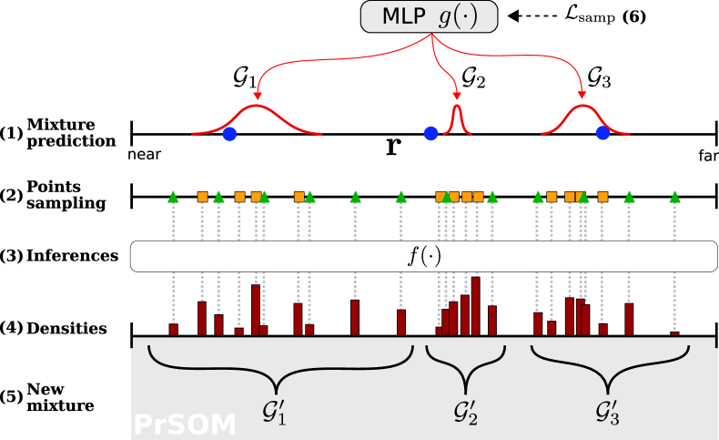
Figure 3: Probabilistic Ray Sampling (PrSamp). Here, $k{=}3$ Gaussians and $m{=}4$ points per Gaussian. Refer to Sec. 3.2 for details.

Prior works [48, 25, 45] demonstrate that for volume rendering, sampling points close to the scene surface improves color estimation (i.e., Eq. 2) while reducing its computational cost due to less $f(\cdot)$ inferences. This is however not trivial here since we lack depth guidance making surface location unknown.

To address this, our probabilistic ray sampling strategy (PrSamp) models the continuous density along each ray as a mixture of 1D Gaussians which then serve as support for points sampling. PrSamp implicitly learns to correlate high mixture values with surface locations, subsequently allowing better sampling with much less points. For example, optimization of a 100m volume requires only 64 points per ray.

Referring to symbols and (steps) in Fig. 3, for each ray $\mathbf{r}$ we first uniformly sample $k$ points (${\color[rgb]{0,0,1}\bullet}$) between near and far bounds. (1) Taking as input the points ${\color[rgb]{0,0,1}\bullet}$ and their corresponding features $\mathbf{W}(\psi({{\color[rgb]{0,0,1}\bullet}}))$, a dedicated MLP $g(\cdot)$ predicts a mixture of $k$ 1D Gaussians $\{\mathcal{G}_{1},\dots,\mathcal{G}_{k}\}$. (2) We then sample $m$ points per Gaussian (${\color[rgb]{1,.5,0}\blacksquare}$) and 32 more points uniformly (${\color[rgb]{0,1,0}\blacktriangle}$) ; which amounts to $N{=}k{\times{}}m{{\color[rgb]{1,.5,0}\blacksquare}}{+}32{{\color[rgb]{0,1,0}\blacktriangle}}$ points. The addition of uniform points is essential to explore the scene volume and prevent $g(\cdot)$ from falling into local minima. (3) All points are then passed to $f(\cdot)$ in Eq. 1 for volume rendering of color $\hat{C}(\mathbf{r})$ and depth $\hat{D}(\mathbf{r})$. (4) Intuitively, the densities $\{\sigma_{1},\dots,\sigma_{N}\}$ inferred by $f(\cdot)$ are cues for 3D surface locations, which we use to update our mixture of Gaussians. To solve the underlying points-Gaussians assignment problem (5) we rely on Probabilistic Self-Organizing Maps (PrSOM) from [2]. In a nutshell, PrSOM assigns points to Gaussians from the likelihood of the former to be observed by a set of points while strictly preserving the mixture topology. For each Gaussian $\mathcal{G}_{i}$ and its assigned points $\mathcal{X}_{i}$ , the updated $\mathcal{G}^{\prime}_{i}$ is the average of all points $j\in\mathcal{X}_{i}$, weighted by the conditional probability $p(j/\mathcal{G}_{i})$ defined in [2] and the occupancy probability of $j$.

Finally, (6) the Gaussians predictor $g(\cdot)$ is updated from the mean of KL divergences between the current and the new Gaussians:

$$\mathcal{L}_{\text{gauss}}=\frac{1}{k}\sum_{i}^{k}\text{KL}(\mathcal{G}_{i}||\mathcal{G}^{\prime}_{i})\,.$$ (5)

To further enforce one Gaussian on the visible surface, we also minimize distance between depth and closest Gaussian:

$$\mathcal{L}_{\text{surface}}=\min_{i}(||\mu(\mathcal{G}^{\prime}_{i})-\hat{D}(\mathbf{r})||_{1})\,.$$ (6)

The complete loss is the sum: $\mathcal{L}_{\text{samp}}=\mathcal{L}_{\text{gauss}}+\mathcal{L}_{\text{surface}}$.

In practice, we use $k=4$ Gaussians and $m=8$ points per Gaussians, leading to only $N=64$ points per ray. The pseudo code is shown in Algorithm 1. We ablate parameters in Sec. 4.4.

3.3 Spherical U-Net (SU-Net)

By definition, the validity domain of $f(.)$ is restricted to the feature volume $\mathbf{W}(.)$ which for a standard U-Net is the camera FOV, thus preventing estimation of color and depth (Eqs. 2,3) outside of the FOV where features cannot be extracted. This is unsuitable for scene reconstruction.

Instead, we equip our SU-Net with a decoder convolving in the spherical domain. Because spherical projection induces less distortion than its planar counterpart [62] we may enlarge the FOV (typically, approx. $120^{\circ}$) to hallucinate color and depth beyond the input image FOV.

At the bottleneck, the encoder features are mapped to an arbitrary sphere with $\psi(.)$ and passed to our spherical decoder. To cope with wide feature space at low cost, we employ light-weight dilated convolutions in the spherical decoder and adapt the standard U-Net multi-scale skip-connections simply by mapping features with $\psi(.)$.

In practice, we map a 2D pixel $[x,y]^{\top}$ to its normalized latitude-longitude spherical coordinates $[\theta,\phi]$. Considering $\begin{bmatrix}\mathcal{r}_{x},\mathcal{r}_{y},1\end{bmatrix}^{\top}{\sim}\text{K}^{-1}\begin{bmatrix}x,y,1\end{bmatrix}^{\top}$ a ray passing through said pixel and the camera center. The projection writes:

$$\psi\begin{pmatrix}x\\ y\end{pmatrix}{=}\begin{pmatrix}\theta\\ \phi\end{pmatrix}{=}\begin{pmatrix}\pi-\arctan(\mathcal{r}_{x}^{-1})\\ \arccos(-\mathcal{r}_{y}/r)\end{pmatrix}$$ (7)

where $r=\sqrt{\mathcal{r}_{x}^{2}+\mathcal{r}_{y}^{2}+1}$. When inputted in the decoder, $[\theta,\phi]$ are discretized uniformly and features stored in a tensor that covers an arbitrary large FOV.

3.4 Scene reconstruction scheme

With prior sections, SceneRF is now equipped with novel depth synthesis capability that allows us to synthesize depth that significantly diverges from the source input position. We use this ability to frame scene reconstruction as the composition of multiple novel depth views.

As illustrated in Fig. 4, given an input frame we synthesize novel depths along an imaginary straight path, uniformly every $\rho$ meters up to a given distance. At each position, we also vary the horizontal viewing angles $\Phi{=}\{-\phi,0,\phi\}$.

The synthesized depths are then converted to TSDF using [83] and the overall scene TSDF for voxel $v$ is obtained from the minimum of all: $\text{V}(v)=\text{TSDF}_{\text{argmin}_{i}|\text{TSDF}_{i}(v)|}(v)$, where $i$ spans all synthesized depths. Traditionally, a voxel TSDF is the weighted average of all TSDFs [11, 49], but we empirically show (see Sec. C.2) that using the minimum leads to better results. We conjecture that this relates to the linearly increasing depth error with distance.

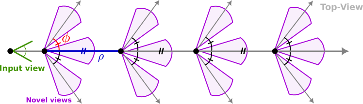
Figure 4: Reconstruction scheme. Given an input image, we fuse the TSDF of the synthesized novel depth/views uniformly sampled along an imaginary path, at varying angles.

4 Experiments

We evaluate SceneRF on two primary tasks, namely novel depth synthesis and scene reconstruction, and novel view synthesis which we refer as ‘subsidiary task’ because it is not used for scene reconstruction. While we do not use 3D data, we need it for evaluation, and thus report results on SemanticKITTI [4, 18] and BundleFusion [13] for all three tasks. Each dataset holds unique challenges. SemanticKITTI has large driving scenes ($\approx$100m deep) and the image sequences are captured from a forward-facing camera which offers little viewpoint variations. Instead, BundleFusion has shallow indoor scenes ($\approx$10m) with sequences exhibiting large lateral motion. Since we first address self-supervised monocular scene reconstruction from RGB images, we detail our non-trivial adaptation of monocular reconstruction baselines [8, 9, 35] (Sec. 4.1).

We always use $k=4$ gaussians and $m=8$ points per Gaussians in PrSamp (Sec. 3.2) but vary novel depth/view sampling for reconstruction (Sec. 3.4). Specifically, we sample views every $\rho=0.5$m for up 10m at angles $\Phi=\{-10,0,+10\}$ for SemanticKITTI, and use $\rho=0.2$m for up to 2.0m with $\Phi=\{-20,0,+20\}$ for BundleFusion.

Method	SemanticKITTI										BundleFusion
	Novel depth synthesis							Novel view synthesis			Novel depth synthesis							Novel view synthesis
Abs Rel$\downarrow$	Sq Rel$\downarrow$	RMSE$\downarrow$	RMSE log$\downarrow$	$\delta$1$\uparrow$	$\delta$2$\uparrow$	$\delta$3$\uparrow$	LPIPS$\downarrow$	SSIM$\uparrow$	PSNR$\uparrow$	Abs Rel$\downarrow$	Sq Rel$\downarrow$	RMSE$\downarrow$	RMSE log$\downarrow$	$\delta$1$\uparrow$	$\delta$2$\uparrow$	$\delta$3$\uparrow$	LPIPS$\downarrow$	SSIM$\uparrow$	PSNR$\uparrow$
MonoDepth2 [21]	0.5259	7.113	14.43	1.0292	10.44	26.32	41.43	0.623	0.166	9.61	0.3205	0.562	0.879	0.4080	44.98	76.31	91.05	0.537	0.492	11.15
MonoDepth2 + LaMa [68]	0.4086	5.101	12.14	0.8472	30.93	49.50	62.65	0.489	0.418	15.32	0.3937	0.954	1.155	0.4538	46.43	75.10	88.79	0.338	0.794	20.80
SynSin [75]	0.3611	3.483	8.824	0.4290	52.61	74.56	86.50	0.519	0.375	14.86	0.2360	0.174	0.522	0.2992	57.08	84.71	95.53	0.627	0.597	13.48
PixelNeRF [81]	0.2364	2.080	6.449	0.3354	65.81	85.43	92.90	0.489	0.466	15.80	0.6029	2.312	1.750	0.5904	46.34	72.38	83.89	0.351	0.822	20.51
MINE [34]	0.2248	1.787	6.343	0.3283	65.87	85.52	93.30	0.448	0.496	16.03	0.1839	0.098	0.386	0.2386	65.53	91.78	98.21	0.377	0.763	20.60
VisionNerf [39]	0.2054	1.490	5.841	0.3073	69.11	88.28	94.37	0.468	0.483	16.49	0.5958	2.468	1.783	0.5586	55.47	79.29	86.68	0.332	0.831	20.51
SceneRF	0.1681	1.291	5.781	0.2851	75.07	89.09	94.50	0.476	0.482	16.46	0.1766	0.094	0.368	0.2100	72.71	94.89	99.23	0.323	0.853	25.07

Table 1: Novel depth/view synthesis. We outperform all on our main task of novel depth, and perform on par on the subsidiary novel view task. Note the large $\delta{}1$ gaps, in particular w.r.t. PixelNerf from which we depart from. (val. sets)

Datasets.

SemanticKITTI [4] has pairs of outdoor geolocalized images with voxelized lidar scans of 256x256x32 with 0.2m voxel, with free/occupy labels. We use the standard train/val split as in [8, 4] and left-crop RGB images to 1220x370. We train SceneRF with successive frames spanning $\approx$10m while ensuring a minimum of 0.4m distance between two frames. This results in 10,270 training sequences. We evaluate novel view at 1:3 resolution and novel depth at 1:2 against sparse lidar projection.
BundleFusion [13] has indoor scenes captured with a handheld device. It has RGB-D images of $640{\times{}}480$ each with an estimated 6-DOF pose. We drop every other frame to increase diversity, i.e. getting 9733 images split in sequences of 17 frames. The middle frame serves as input and remaining ones for supervision. We select 7 of the 8 scenes for training and 1 as validation. We evaluate at 1:2 resolution.

Metrics.

To measure our reconstruction quality, we use the intersection over union (IoU), precision, and recall of occupied voxels. For novel depth estimation, we choose usual metrics [21]: relative error absolute (Abs Rel) or squared (Sq Rel), root mean squared error (RMSE), mean $\log_{10}$ error (RMSE log), threshold accuracies ($\delta$1, $\delta$2, $\delta$3). As a common practice, depth is capped to 80m in SemanticKITTI and 10m in BundleFusion. Following [34], we measure the quality of synthesized RGB images with: Structural Similarity Index (SSIM) [74], PSNR, and LPIPS perceptual similarity [87].

Training setup.

SceneRF trains end-to-end minimizing $\mathcal{L}_{\text{total}}=\mathcal{L}_{\text{rgb}}+\mathcal{L}_{\text{reproj}}+\mathcal{L}_{\text{samp}}$ where $\mathcal{L}_{\text{rgb}}$ is the standard L2 photometric reconstruction loss of NeRFs [57, 45, 81]. We report results for 50 epochs training with batch size of 4 and initial learning rate of 1e-5 with exponential decay at each epoch with gamma $0.95$. Training was conducted on 4 Tesla v100 GPUs, amounting to ${\approx}5$ days.

4.1 Baselines

Novel depth/views. Despite the bustling NeRF field, there are in fact few single-view NeRFs. We select 3 of them among the best open-sourced ones for novel depths/views synthesis: PixelNeRF [81], VisionNeRF [39], MINE [34]. Similar to us, all train with images and poses. We also compare against state-of-the-art 3D-aware GAN, namely SynSin [75] for which novel depths are obtained by applying its depth regressor on novel views. Finally, to account for natural baselines we evaluate against monocular depth estimation, here MonoDepth2 [21], where novel depths (views) are the reprojection of the (colored) point cloud derived from the input view and estimated depth map. As such novel views/depths are inevitably sparse we also report ‘MonoDepth2 + LaMa’ where novel views of MonoDepth2 baseline are inpainted with LaMa [68] and novel depth is obtained from running MonoDepth2 again.

Scene reconstruction. For monocular scene reconstruction, we consider 4 baselines being: MonoScene [8], LMSCNet${}^{\text{rgb}}$ [60], 3DSketch${}^{\text{rgb}}$ [9], AICNet${}^{\text{rgb}}$ [35]. The baselines with ${}^{\text{rgb}}$ are RGB-inferred version from [8]. Since all baselines require geometric supervision from depth sensors, we report ‘3D’ and ‘Depth’ supervision along our ‘Image’ supervision. This is further detailed in Sec. 4.3.

Method	Supervision			SemanticKITTI			BundleFusion
	3D	Depth	Image	IoU	Prec.	Rec.	IoU	Prec.	Rec.
MonoScene [8]	✓			37.14	49.90	59.24	30.15	35.07	68.51
LMSCNet${}^{\text{rgb}}$ [60]		✓		12.08	13.00	63.16	14.91	25.22	31.15
3DSketch${}^{\text{rgb}}$ [9]		✓		12.01	12.95	62.31	16.88	25.82	32.76
AICNet${}^{\text{rgb}}$ [35]		✓		11.28	11.84	70.89	15.99	25.20	30.41
MonoScene [8]		✓		13.53	16.98	40.06	19.00	22.51	54.91
MonoScene* [8]			✓	11.18	13.15	40.22	17.20	21.88	44.59
SceneRF			✓	13.84	17.28	40.96	20.16	25.82	47.92

* Here, MonoScene is supervised by depth predictions of [21] trained with ground-truth poses.

Table 2: Scene reconstruction. Despite being the only self-supervised method, we outperform all ‘Depth’ supervised baselines. Refer to Sec. 4.3 for supervision details.

Method	SemanticKITTI										BundleFusion
	Novel depth synthesis							Novel view synthesis			Novel depth synthesis							Novel view synthesis
AbsRel$\downarrow$	SqRel$\downarrow$	RMSE$\downarrow$	RMSElog$\downarrow$	$\delta$1$\uparrow$	$\delta$2$\uparrow$	$\delta$3$\uparrow$	LPIPS$\downarrow$	SSIM$\uparrow$	PSNR$\uparrow$	AbsRel$\downarrow$	SqRel$\downarrow$	RMSE$\downarrow$	RMSElog$\downarrow$	$\delta$1$\uparrow$	$\delta$2$\uparrow$	$\delta$3$\uparrow$	LPIPS$\downarrow$	SSIM$\uparrow$	PSNR$\uparrow$
SceneRF	0.1681	1.291	5.781	0.2851	75.07	89.09	94.50	0.476	0.482	16.46	0.1766	0.094	0.368	0.2100	72.71	94.89	99.23	0.323	0.853	25.07
w/o $\mathcal{L}_{\text{rgb}}$	0.1801	1.480	6.347	0.3085	72.15	87.56	93.66	-	-	-	0.1769	0.084	0.374	0.2043	71.75	95.82	99.79	-	-	-
w/o $\mathcal{L}_{\text{reproj}}$	0.2115	1.706	6.133	0.3059	69.10	87.55	94.13	0.491	0.481	16.42	0.2168	0.144	0.454	0.2577	64.99	90.47	97.72	0.328	0.852	24.82
w/o SU-Net	0.1758	1.386	5.908	0.2967	73.91	88.27	94.01	0.464	0.480	16.40	0.2449	0.167	0.488	0.3263	59.77	85.84	94.63	0.461	0.730	14.29
w/o PrSamp	0.1858	1.301	5.844	0.2936	71.85	88.73	94.24	0.505	0.471	16.43	0.1825	0.100	0.385	0.2125	70.69	94.10	98.78	0.317	0.730	25.15
Freeze $\sigma$ $\mathcal{L}_{\text{rgb}}$	0.1750	1.366	6.029	0.2962	73.42	88.28	94.14	0.494	0.476	16.42	0.2081	0.131	0.423	0.2362	67.55	92.68	98.42	0.342	0.850	24.80
$\mathcal{L}_{\text{rgb}}$ on S + T	0.1966	1.484	5.993	0.2991	70.36	88.35	94.07	0.486	0.478	16.40	0.1942	0.134	0.409	0.2270	70.78	93.73	98.18	0.357	0.838	24.71

Table 3: Architecture ablation on the validation set. All components contribute to yielding better results for our primary task of novel depth synthesis, with mixed results on novel view synthesis. Details are in Sec. 4.4.

4.2 Novel depth synthesis

To first evaluate the quality of our novel depths/views, given an input image we synthesize depth/views at the position of all frames in the sequence except for the input one.

From Tab. 1, for the task of novel depth synthesis we rank first on all metrics with a comfortable margin. In particular, one may note the large gaps on AbsRel and $\delta{}$-metrics as they are challenging metrics. It is also noticeable that we significantly improve over PixelNeRF, from which we depart, demonstrating the benefit of our design choices. For example, we get an improvement of +9.26 and +26.37 for $\delta{}1$ on SemanticKITTI and BundleFusion, respectively, w.r.t. PixelNeRF. Unsuprisingly, we outperform very significantly baselines using monocular depth estimation (i.e., MonoDepth2) or 3D-GAN (i.e., SynSin) which we ascribe to radiance volumes preserving 3D-aware consistency.

Though of least importance for scene reconstruction, Tab. 1 also shows that SceneRF is roughly on par with the best methods on the subsidiary task of novel views synthesis where, notably, we always improve over PixelNeRF.

In Sec. 4.3, we primarily show novel depths and the subsidiary novel views for varying input frames, multiple positions and angles w.r.t. the input frame position. For all, novel depths are visually outperforming the baselines. In particular, we note the sharper depth edges and the better quality at far when zooming in. When varying the viewing angle (i.e., $-10^{\circ}$ or $+10^{\circ}$) we note also fewer edge artefacts than baselines, which is even more striking for the outdoor example. Please also refer to the supplemental video.

4.3 3D reconstruction results

To evaluate reconstruction, we compare against the voxelized 3D groundtruth which is obtained either from the accumulation of lidar scans in SemanticKITTI or the fusion of depth maps in BundleFusion.

Though we do not require depth or 3D for supervision, we still report 3 supervision setups in Tab. 2: (i) ‘3D’ where baselines are trained with full 3D groundtruth. (ii) ‘Depth’ using as supervision the TSDF fusion [83] of depth sequences from the supervised AdaBins method [5] which we retrain to boost performance. (iii) ‘Image’ where like in SceneRF, we only train self-supervisedly from image sequences. It is important to note that, except for the ’Image’-supervision baseline, all other baselines incorporate some sense of ground truth depth which we do not have.

From Tab. 2, SceneRF is the only original self-supervised baseline that still outperforms all ‘Depth’-supervised baselines on both datasets. This is surprising given the additional geometrical supervision of ‘Depth’ methods. It advocates that SceneRF efficiently self-discovers geometrical cues from image sequences. For more in depth comparison, we also adapt MonoScene [8] to ‘Image’-supervision, using as ground truth the fusion of depth predictions of [21]. SceneRF still outperforms this image-supervised MonoScene by $\approx$ 3 points on BundleFusion. We also report the original ‘3D’-supervised MonoScene, acting as an unreachable upper bound since 3D provides supervision beyond occlusions. In general, The low numbers for ’Depth’ and ’Image’ methods suggest task complexity, indicating potential for future research.

Sec. 4.3 also shows reconstructed 3D meshes for sample inputs. Results are better seen when zooming in and in supplementary video. On both datasets SceneRF produces better reconstruction results with less artefacts, especially on vegetation and sidewalk on SemanticKITTI and general scene structure on BundleFusion.

Input	Method	3D mesh (w/ our recons. scheme)	Novel depth			Novel view
			$+1$m, $0^{\circ}$	$+3$m, ${-}10^{\circ}$	${+}5$m, ${+}10^{\circ}$	${+}5$m, ${+}10^{\circ}$
	PixelNeRF
	MINE
	VisionNeRF
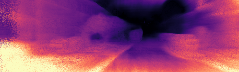
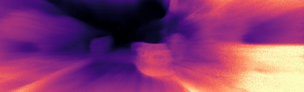
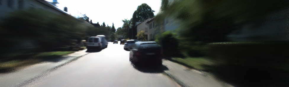
	SceneRF
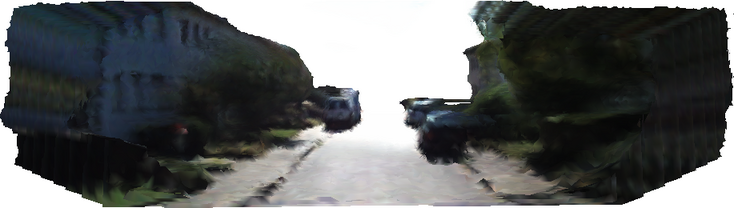
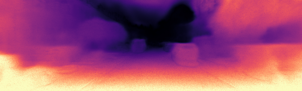
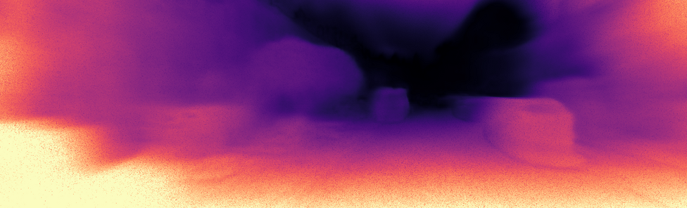
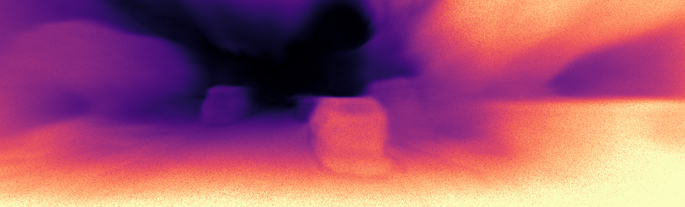
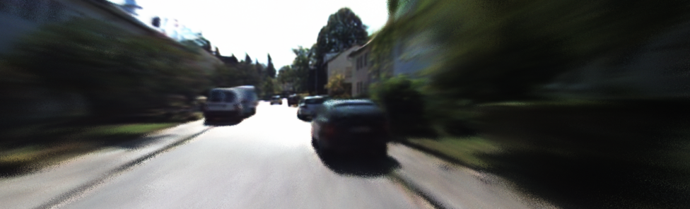
gray!50			$+0.2$m, $0^{\circ}$	$+0.2$m, ${-}20^{\circ}$	${+}0.4$m, ${+}20^{\circ}$	${+}0.4$m, ${+}20^{\circ}$
	PixelNeRF
	MINE
	VisionNeRF
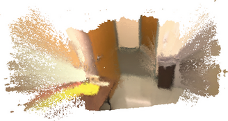
	SceneRF
gray!50

Figure 5: Qualitative results on SemanticKITTI and BundleFusion. For each row, we report novel depths/views at varying positions and viewing angles w.r.t. the input frame. We note that our depths are sharper and better at-far distances. To produce 3D meshes, all — even baselines — use our scheme for reconstruction (Sec. 3.4). On both datasets, our reconstruction is evidently better than others. Please zoom in and refer to video in supplementary for better qualitative judgement.

4.4 Ablation studies

Architectural components.

Tab. 3 reports novel depth/view synthesis of SceneRF when removing the rgb loss ($\mathcal{L}_{\text{rgb}}$), reprojection loss ($\mathcal{L}_{\text{reproj}}$, Eq. 4), Spherical U-Net (SU-Net, Sec. 3.3), or Probabilistic Sampling (PrSamp, Sec. 3.2). Without SU-Net, we use a standard U-Net of similar capacity where $\psi(.)$ is a simple cartesian projection. Without PrSamp, we revert to standard hierarchical sampling [45, 81], using the same number of inferences for a fair comparison.

In a nutshell, all our components contribute to the best novel depth synthesis metrics. In particular, $\mathcal{L}_{\text{reproj}}$ and PrSamp improve significantly the absolute relative error and the $\delta{}1$, showing a beneficial effect on close range depth estimation. For the subsidiary task of novel view synthesis, our components have mixed effects showing that depth improvement comes at the cost of slightly lower image reconstruction.

Probabilistic Ray Sampling (Sec. 3.2).

It is tempting to assume that PrSamp would better approximate the underlying density volume with more Gaussians or more sampled points, thus yielding better results. This is proven wrong in Tab. 4 where we vary the number of Gaussians ($k$) and points sampled per Gaussian ($m$). The best results are with $k{=}4$ and $m{=}8$. We conjecture this relates to the radiance field not being able to optimize too many surfaces per ray. Fewer Gaussians also preserve computational cost, more Gaussians introduce noise with fewer points per Gaussian.

We now compare PrSamp ($k{=}4$ and $m{=}8$) against other samplings. First, we train SceneRF${}^{\text{MN360}}$ where PrSamp is replaced by the sampling of MipNerf360 [3]. Our SceneRF (i.e., using PrSamp) outperforms SceneRF${}^{\text{MN360}}$ on all metrics and datasets, with $\delta{}1$/$\delta{}2$/$\delta{}3$ of +6/+3/+2 on SemanticKITTI and +5/+4/+2 on BundleFusion. We conjecture that this relates to our uniform sampling (${\color[rgb]{0,1,0}\blacktriangle}$, Sec. 3.2) which encourages ray exploration, i.e. fighting view ambiguity, while MN360 coarse-to-fine distillation prevents escaping from invalid minima. Importantly, note that MN360 uses 96 inferences (64 proposal+32 NeRF) and PrSamp only 64 (32+32). Second, we depart from original VisionNerf in Tab. 1 and train VisionNerf${}^{\text{PrSamp}}$ where hierarchical sampling is replaced by our PrSamp, which proves to improve $\delta{}1$/$\delta{}2$/$\delta{}3$ by +3.9/+0.1/+0.1 on SemanticKITTI.

Explicit depth optimization ($\mathcal{L}_{\text{reproj}}$).

Besides performance in Tab. 3, it is reasonable to question the need of explicit depth optimization as NeRF-based methods can implicitly estimate depth. We argue that $\mathcal{L}_{\text{rgb}}$ and $\mathcal{L}_{\text{reproj}}$ pursue slightly different objectives since $\mathcal{L}_{\text{rgb}}$ optimizes the rendered image by adjusting point density color $\mathbf{c}$ and $\sigma$ w.r.t. source frame ($I_{j}$ in Fig. 2), while $\mathcal{L}_{\text{reproj}}$ optimizes reprojection of source on target ($I_{j-1}$ in Fig. 2) but solely by adjusting depth with $\sigma$. In Tab. 3 bottom we verify the complementarity of the two losses. First, we ‘Freeze $\sigma$ in $\mathcal{L}_{\text{rgb}}$’ to separate both optimization objectives, which performs worse (${-}4$ on $\delta_{1}$). Second, we verify that using target in $\mathcal{L}_{\text{reproj}}$ does not provide an unfair edge by removing $\mathcal{L}_{\text{reproj}}$ and replacing $\mathcal{L}_{\text{rgb}}$ with ‘$\mathcal{L}_{\text{rgb}}$ on source+target’ — which also drops performance (${-}6$ on $\delta_{1}$). In Appendix B, we also show that $\mathcal{L}_{\text{reproj}}$ can boost the geometric ability of other NeRFs.

$k$	$m$	Abs Rel$\downarrow$	Sq Rel$\downarrow$	RMSE$\downarrow$	RMSE log$\downarrow$	$\delta$1$\uparrow$	$\delta$2$\uparrow$	$\delta$3$\uparrow$
1	32	0.1850	1.358	5.956	0.2940	71.38	88.73	94.51
2	16	0.1788	1.327	5.889	0.2878	72.68	88.90	94.70
4	4	0.1845	1.371	5.878	0.2940	71.62	88.59	94.51
	8	0.1717	1.309	5.696	0.2809	75.01	89.35	94.76
	16	0.1664	1.319	5.980	0.2894	74.58	88.48	94.17
8	4	0.1768	1.311	5.824	0.2910	72.86	88.60	94.42
	8	0.1697	1.311	5.794	0.2873	74.59	88.71	94.34

Table 4: PrSamp ablation on Sem.KITTI (val). We vary number of Gaussians ($k$) and points per Gaussian ($m$).

Spherical U-Net (Sec. 3.3).

Tab. 3 ‘w/o SU-Net’ highlights the benefit of our SU-Net. We complement this study, by comparing planar (i.e., standard decoder) and spherical decoder of different horizontal FOV. We experiment with planar-80^∘/planar-120^∘/spherical-80^∘/spherical-120^∘, getting respectively 17.66/17.25/17.67/17.17 for Abs Rel metric (lower is better) and 73.78/74.23/73.46/75.01 for $\delta 1$ (higher is better). Larger FOV seems to always improve, but our spherical decoder reaches the best results — presumably because it induces less projection distortion.

Figure 6: Performance vs. input view distance on SemanticKITTI. Novel depth quality drops as distance increases due to lower overlaps of FOV with the input view.

Performance beyond input FOV.

Different than generative methods, like GAN, a minimum FOV overlaps between the input and the novel view is needed to estimate relevant features. We quantify this on novel depth in Fig. 6 showing that all metrics drop significantly as a function of the novel view distance although SceneRF is consistently better. For novel view synthesis, we evaluate the quality of the generated unseen pixels using ‘masked metrics’ in Tab. 5, i.e., evaluating only pixels not seen in the input frame. Here again, SceneRF is far better than any other baselines.

		Novel depth synthesis							Novel view synthesis
	Method	AbsRel$\downarrow$	SqRel$\downarrow$	RMSE$\downarrow$	RMSElog$\downarrow$	$\delta$1$\uparrow$	$\delta$2$\uparrow$	$\delta$3$\uparrow$	LPIPS$\downarrow$	SSIM$\uparrow$	PSNR$\uparrow$
SemKITTI	PixelNeRF	0.5145	8.057	14.835	0.843	9.10	26.68	47.58	N / A		33.48
	MINE	0.3869	6.099	13.105	0.656	25.41	50.43	67.55			33.47
	VisionNerf	0.4831	7.556	14.573	0.825	14.50	34.43	52.44			33.41
	SceneRF	0.3056	4.187	9.980	0.447	44.32	69.56	81.40			33.91
Bun.Fusion	PixelNeRF	3.2717	20.369	5.277	1.441	4.48	10.40	15.75	N / A		22.18
	MINE	0.2047	0.112	0.388	0.246	62.77	90.90	98.24			25.47
	VisionNerf	3.3925	20.645	5.360	1.453	4.43	10.11	14.67			21.63
	SceneRF	0.1848	0.092	0.343	0.211	70.06	94.00	99.18			25.90

Table 5: Masked metrics. We calculate the metrics for pixels that are not visible in the input image, highlighting the superiority of SceneRF compared to the baselines.

* Monodepth2 is trained with GT poses for fair comparison with our setting.

Table 6: Variations of scene reconstruction. We compare SceneRF against reconstruction with AdaBins [5] (depth-supervised) or Monodepth2 [21] (self-supervised), and also report result w/o our Reconstruction Scheme (Sec. 3.4). Note that, conversely to SceneRF, baselines use TSDF of the depth from the input view.

Scene reconstruction (Sec. 3.4).

We study variations of our scene reconstruction scheme in Tab. 7. In the first 3 rows, we evaluate reconstruction using a single depth map at the input frame with the best monocular depth estimation methods being: AdaBins [5] (depth-supervised), Monodepth2 [21], and SceneRF w/o reconstruction scheme. AdaBins is the only that requires depth and logically outperforms others on SemKITTI where scene are deep and Lidar provides an unfair supervision edge. On BundleFusion, SceneRF however outperforms AdaBins by ${\approx{}}+2$ IoU points which is remarkable as it is self-supervised. SceneRF also reaches best performance among all self-supervised methods with roughly +3 and +6 IoU w.r.t. Monodepth2 [21] on SemKITTI and BundleFusion, respectively. SceneRF also outperforms reconstructions from SynSin and all other NeRFs by a few points on both datasets. In Appendix A, we also study the effect of varying steps ($\rho$) and rotations ($\Phi$) in our reconstruction scheme.

5 Discussion

To the best of our knowledge, SceneRF is the first method to handle complex cluttered scenes. Still, self-supervised monocular scene reconstruction is yet in its early steps, and we discuss here some remaining challenges.

Input	3D mesh	Novel depth		Novel view
		$+1$m, $0^{\circ}$	$+3$m,${-}10^{\circ}$	${+}3$m,${-}10^{\circ}$

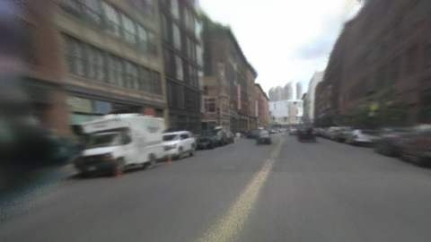
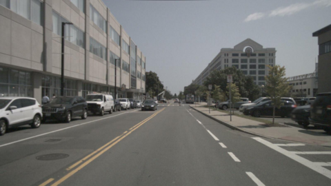
Figure 7: nuScenes generalization. (train on SemKITTI)

Features compression.  A drawback of our planar${\mapsto}$spherical mapping of SU-Net is that it induces spatial compression. An intuitive example is when input/output are of same size, since features will project on a smaller spatial portion of the output feature map. A simple workaround would be to increase output size but this would come at higher memory cost.

Inference time.  Despite fewer inferences thanks to our PrSamp, depth synthesis is still time-consuming due to per-point inference — which limits applicability. We conjecture that ray inference [64] could be beneficial here.

Generalization.  To overcome the highly ill-posed problem of reconstruction from a single image, NeRF-based methods rely on strong priors learned on the training set. This poses inevitable issues for across domains generalization (e.g., beyond driving scenes). Still, in Fig. 7 we show that when training on SemanticKITTI, SceneRF exhibits some generalization capability to the unseen nuScenes images [6] despite a large gap (Germany$\mapsto$USA, different camera setup, etc.).

Direct Field Reconstruction.  As SceneRF uses fused synthesized depths (Sec. 3.4) which are proxies of the radiance field, this suggests that reconstruction could be achieved directly. While our experiments show that using alpha/sigma to reconstruct 3D scene is not straightforward, we believe an interesting avenue for research is to seek direct extraction of surfaces from the radiance field.

Acknowledgment  The work was partly funded by the French project SIGHT (ANR-20-CE23-0016) and conducted in the SAMBA collaborative project, co-funded by BpiFrance in the Investissement d’Avenir Program. It was performed using HPC resources from GENCI–IDRIS (Grant 2021-AD011012808, 2022-AD011012808R1, and 2023-AD011014102). We thank Fabio Pizzati and Ivan Lopes for their kind proofreading and all Astra-vision group members of Inria Paris for the insightful discussions.

We begin by discussing the broader impact and ethics of our work. We then present additional ablations in Appendix A along with further implementation details in Appendix C. After that, we demonstrate in Appendix B that $\mathcal{L}_{\text{reproj}}$ improves all baselines. Details of the baselines are presented in Appendix D. Finally, we show additional qualitative results in Appendix E. The supplementary video, which is available at https://astra-vision.github.io/SceneRF/, allows better evaluation of our method.

Broader impact, Ethics.

The promotion of self-supervised monocular 3D reconstruction contributes to alleviating the needs of costly data acquisition and labeling campaigns. On the long term, this also paves the way to 3D algorithms training directly on video sequences – easier to collect and significantly more diverse than existing 3D datasets. A by-product is that it would contribute to improving generalization of 3D reconstruction. While there are no ethical concerns specific to our proposed method, we note that all methods estimating 3D from 2D are far less precise than those leveraging depth sensors (e.g., lidar, depth cameras, stereo, etc.). When it comes to safety-critical applications, like autonomous driving, we argue for use of redundant sensors.

Appendix A Additional ablations

Sampling strategy.

In Tab. 7 we illustrate the effect of varying step ($\rho$) and angle ($\phi$) when sampling novel depths/views in our scene reconstruction scheme (Sec. 3.4). As noted in Sec. 4, the views are sampled up to a distance of 10m on SemanticKITTI [4] and 2m on BundleFusion [13]. Increasing the number of synthesized depth maps (i.e., reducing the step $\rho$) and varying the angle ($\phi$) generally improves the IoU score. However, excessively large angle ($\geq$ 20^∘ on SemanticKITTI [4], $\geq$ 30^∘ on BundleFusion [4]) tends to degrade performance since the synthesized angle diverges significantly from the available angles during training. This is particularly pertinent in the context of autonomous driving setups with front-facing cameras, where there is limited peripheral supervision.

step (m)	rot. (deg.)	IoU	Prec.	Rec.
w/o sampling		11.80	19.91	22.47
0.25	-10 / 0 / +10	13.73	16.98	41.78
black!10 0.5	-10 / 0 / +10	13.84	17.28	40.96
1.0	0	13.08	18.56	30.68
1.0	-10 / 0 / +10	13.40	17.27	37.43
1.0	-20 / 0 / +20	13.37	16.73	39.97
1.0	-30 / 0 / +30	13.24	16.40	40.73
2.0	-10 / 0 / +10	13.35	17.41	36.35

(a) SemanticKITTI [4]

step (m)	rot. (deg.)	IoU	Prec.	Rec.
w/o sampling		17.33	20.13	55.43
0.1	-20 / 0 / +20	20.34	25.70	49.28
0.2	0	18.76	26.43	39.28
0.2	-10 / 0 / +10	19.94	25.80	46.76
black!10 0.2	-20 / 0 / +20	20.16	25.82	47.92
0.2	-30 / 0 / +30	19.98	25.90	46.64
0.3	-20 / 0 / +20	19.84	25.84	46.09

(b) BundleFusion [13]

Table 7: Sampling for reconstruction. Performance of our reconstruction scheme when varying our sampling steps ($\rho$) and angles ($\phi$) (val. set). The highlighted row is our main setup.

BundleFusion evaluation on more sequences.

For completeness, we retrain on 6 sequences (apt0, apt1, apt2, office1, office2, office3) with 2 validation sequences of unseen rooms (copyroom, office0) to show generalization. The results are shown in Tab. 8 and show that SceneRF still surpasses all baselines on all 10 metrics except LPIPS. This is on par with Tab. 1.

	Novel depth synthesis							Novel view synthesis
Method	Abs Rel$\downarrow$	Sq Rel$\downarrow$	RMSE$\downarrow$	RMSE log$\downarrow$	$\delta$1$\uparrow$	$\delta$2$\uparrow$	$\delta$3$\uparrow$	LPIPS$\downarrow$	SSIM$\uparrow$	PSNR$\uparrow$
PixelNeRF	0.6332	2.370	1.786	0.5722	48.01	73.82	84.09	0.421	0.770	19.36
MINE	0.1712	0.085	0.368	0.2214	70.74	93.42	98.46	0.430	0.714	20.21
VisionNerf	0.6384	2.813	1.934	0.5721	59.25	78.62	84.37	0.391	0.790	19.67
SceneRF	0.1581	0.069	0.330	0.1921	75.81	96.80	99.66	0.404	0.801	24.02

Table 8: BundleFusion. Train on 6 scenes and evaluate on 2 scenes.

		Novel depth synthesis							Novel view synthesis
Method	$\mathcal{L}_{\text{reproj}}$	Abs Rel$\downarrow$	Sq Rel$\downarrow$	RMSE$\downarrow$	RMSE log$\downarrow$	$\delta$1$\uparrow$	$\delta$2$\uparrow$	$\delta$3$\uparrow$	LPIPS$\downarrow$	SSIM$\uparrow$	PSNR$\uparrow$
PixelNeRF [81]	✗	0.2364	2.080	6.449	0.3354	65.81	85.43	92.90	0.489	0.466	15.80
	✓	0.1986	1.544	5.963	0.3093	70.30	87.19	93.82	0.488	0.481	16.11
MINE [34]	✗	0.2248	1.787	6.343	0.3283	65.87	85.52	93.30	0.448	0.496	16.03
	✓	0.2003	1.599	6.023	0.3070	70.22	86.98	93.89	0.445	0.497	15.96
VisionNerf [39]	✗	0.2054	1.490	5.841	0.3073	69.11	88.28	94.37	0.468	0.483	16.49
	✓	0.1749	1.380	5.643	0.2841	75.77	89.25	94.58	0.432	0.488	16.39

Table 9: Reprojection loss $\mathcal{L}_{\text{reproj}}$ on other baselines. We apply our reprojection loss to other NeRF baselines, showing it boosts performance for all.

Appendix B Effect of $\mathcal{L}_{\text{reproj}}$ on NeRF baselines

In Tab. 9, we apply the reprojection loss $\mathcal{L}_{\text{reproj}}$ (Sec. 3.1.1) to all NeRF baselines, showing that it improves consistently all of them. Again, we argue this is because $\mathcal{L}_{\text{reproj}}$ enforces better density ($\sigma$) in the volume rendering – which has a complementary effect with $\mathcal{L}_{\text{rgb}}$.

Appendix C Additional implementation details

C.1 Probabilistic ray sampling (PrSamp) details

For clarity, in Algorithm 1, we detail the pseudocode of the Probabilistic Ray Sampling (Sec. 3.2).

Input : Ray $\mathbf{r}$.

Param :  Number of Gaussians $k$, and $m$ number of points per Gaussian.

Near and far bounds: $t_{\text{n}}=0.2\text{m}$ and $t_{\text{f}}=100\text{m}$.

Learning rate $lr$ of gradient descend (GD).

Result: Points sampled $\mathcal{P}$

1 $\mathbf{d}\leftarrow\textnormal{{dir}}(\mathbf{r})$

// Uniform sampling (${\color[rgb]{0,0,1}\bullet}$)

2 $\mathcal{I}\leftarrow\{\textnormal{{uniform-samp}}(\text{num=}k,\text{start=}t_{\text{n}},\text{end=}t_{\text{f}})\times\mathbf{d}\}$ $\triangleright$ Points sampling between near and far bounds

// (1) Predicts Gaussians ($\mathcal{G}$) with MLP $g(\cdot)$

3 $\mathcal{G}\leftarrow g\big{(}\big{\{}(\mathbf{x},\mathbf{W}(\psi(\mathbf{x})))\,|\,\forall\mathbf{x}\in\mathcal{I}\big{\}}\big{)}$

// (2) Sample $m$ points from Gaussians (${\color[rgb]{1,.5,0}\blacksquare}$)

4 $\mathcal{P}\leftarrow\emptyset$

5 for $i\leftarrow 1$ to $k$ do

6      $\mathcal{P}\leftarrow\mathcal{P}\cup\textnormal{{gauss-sampling}}(\mathcal{G}_{i},m)$

7      

8 end for

// Sample 32 points uniformly (${\color[rgb]{0,1,0}\blacktriangle}$)

9 $\mathcal{P}\leftarrow\mathcal{P}\cup\{\textnormal{{uniform-samp}}(\text{num=}32,\text{start=}t_{\text{n}},\text{end=}t_{\text{f}})\times\mathbf{d}\}$

// (3)-(4) NeRF inference to compute densities

10 $\sigma\leftarrow\{f(\gamma(\mathbf{x}),\mathbf{d};\mathbf{W}(\psi(\mathbf{x})))_{\sigma}\,|\,\forall\mathbf{x}\in\mathcal{P}\}$ $\triangleright$ Densities from $f(\cdot)$ inferences Eq. 1

// (5) PrSOM point-Gaussian assigment

11 $\alpha\leftarrow\{\textnormal{{alpha-value}}(s,\dots)\,|\,\forall s\in\sigma\}$ $\triangleright$ Compute alpha values from [44] p3

12 $\mathcal{X}\leftarrow\{\textnormal{{PrSOM}}(\mathcal{G},\mathcal{P},\alpha)\}$ $\triangleright$ Applies PrSOM [2]

// (6) Compute new Gaussians from assigned points and update $g(\cdot)$

13 $\mathcal{G}^{\prime}\leftarrow\{(\mu(\mathcal{X}_{i}),\text{std}(\mathcal{X}_{i}))\,|\,\forall i\in\mathbb{N},1<=i<=k\}$

14 $\mathcal{L}_{\text{gauss}}\leftarrow\frac{1}{k}\sum_{i}^{k}\textnormal{{Kullback-Leibler}}(\mathcal{G}_{i}||\mathcal{G}^{\prime}_{i})$

15 $\mathcal{L}_{\text{surface}}\leftarrow\min_{i}(||\mu(\mathcal{G}^{\prime}_{i})-\hat{D}(\mathbf{r})||_{1})$

16 $\mathcal{L}_{\text{total}}\leftarrow\mathcal{L}_{\text{gauss}}+\mathcal{L}_{\text{surface}}$

$g\leftarrow\textnormal{{GD}}^{lr}(g,\nabla\mathcal{L}_{\text{total}})$ $\triangleright$ Applies gradient-descent to update $g(\cdot)$

Algorithm 1 Probabilistic Ray Sampling.

C.2 3D reconstruction details

Fusing TSDFs.

From Sec. 3.4, we fuse individual TSDFs by taking the minimum of their absolute values (‘min’) instead of the more standard average of all TSDFs (‘avg’). We justify this choice, in Tab. 10 showing that using ‘min’ leads to +2.77 IoU. We argue that some surfaces may be better estimated from specific camera locations. Averaging all (‘avg’) has a smoothing effect on $V(\cdot)$ which subsequently reduces accuracy.

Method	IoU	Prec.	Rec.
SceneRF (avg)	11.07	11.81	63.98
SceneRF (min)	13.84	17.28	40.96

Table 10: TSDF fusion strategy comparison on SemanticKITTI [4]. We show that our way of extracting the TSDF described in section 3.4 is better than the traditional way of using the weighted average of TSDFs.

Occupancy grid.

To convert the scene TSDF volume $V(\cdot)$ (cf. Sec. 3.4) into an occupancy grid, we first study the depth estimation error. Comparing 100 frames in Fig. 8 with sparse Lidar ground truth, we note a linear relation between error estimation and ground truth depth. This motivated us to model the occupancy grid $O(\cdot)$ as an adaptive depth threshold:

$$O(v)=1\iff\text{V}(v)<\min(0.25d_{v},4.0)\,,$$ (8)

with $v$ a voxel in V, and $d_{v}$ its distance to the camera origin. We arbitrarily cap the threshold to 4 meters to avoid considering all far voxels as occupied.

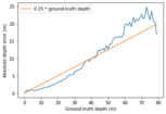
Figure 8: Absolute depth error w.r.t. ground-truth depth. We compute error from 100 randomly selected scenes in the training set, and observe a linear relation between error and distance.

C.3 Network architecture

For 2D features extraction, the encoder is similar to [8], which is based on a pre-trained EfficientNetB7 [69]. The spherical decoder has 5 layers, each of which doubles the input resolution and halves the feature dimension. To make up for the large amount of empty space that comes with increasing the field of view, we augment the receptive field by putting three ResNet blocks with dilation sizes of 1, 2, and 3 in each layer. The skip connections (described in Sec. 3.3) are used between the encoder and decoder at the corresponding scale.

C.4 BundleFusion – 3D ground-truth

We seek to generate for each input frame the 3D ground-truth occupancy grid. To do this, we use the camera parameters and define a volume of (4.8m, 4.8m, 3.84m) in front of the camera. The origin is set at (-2.4m, -2.4m, 0m) such that the camera is in the middle of one side of the volume and pointing inward. We then combine the depth maps to create the TSDF volume with a voxel size of 0.04m, resulting in a TSDF grid of size (120, 120, 96). Finally, the occupancy grid is obtained by thresholding the TSDF grid.

Appendix D Baselines details

We re-train all baseline networks, including the novel depth/view synthesis (Sec. D.1) and scene reconstruction baselines (Sec. D.2). We provide the reader with additional details about our baselines.

D.1 Novel depth/views baselines

We train our method and baselines using AdamW [42] optimizer on 4 Tesla V100 32g with learning rate of 1e-5 for 50 epochs. For each baseline, we rely on the recommended learning rate scheduler and number of positional encoding frequencies. For our network, since we build on PixelNeRF [81], we use its scheduler and number of frequencies. The ray batch size was 1200 for Semantic KITTI [4] and 2048 for BundleFusion [13]. The training time was around 5 days per network. Additional information about the baselines implementations is provided below.

PixelNeRF [81].

We use the official implementation. Following the official sampling strategy, we sample 96 points per ray, consisting of 64 coarse points, which are used to sample 16 fine points hierarchically and 16 points around the estimated depth.

MINE [34].

We use the official implementation. To balance memory cost, we use the 32 planes version.

VisionNeRF [39].

We use the official implementation. To balance memory cost again, we sample 96 points (32 coarse, 64 fine) which is more than for SceneRF.

D.2 Scene reconstruction baselines

Only MonoScene is a monocular baseline. To better compare with the literature, we follow the recommendation of MonoScene authors [8] and compare against the ${}^{\text{rgb}}$ versions of popular semantic scene completion baselines: LMSCNet [60], 3DSketch [9] and AICNet [35]. More in depth, to convert the sequence of depths into 3D label to train the scene reconstruction baselines, we use the Adabin [5] model to predict the depth for each image and fuse all depths into a single TSDF volume, then turned into an occupancy grid with the same reconstruction scheme as for SceneRF (see Sec. C.2). For all, the mesh is obtained with the traditional marching cubes [41].

Appendix E Additional qualitative results

Voxelized reconstructions on SemanticKITTI [4].

Fig. 9 shows the voxelized reconstructions comparing our self-supervised SceneRF with the Depth-supervised version of MonoScene [8] which relies on AdaBins [5] trained with Lidar ground truth. Notably, despite less supervision the predictions of SceneRF align closely with those of MonoScene in terms of overall scene architecture, object shapes, and positioning. Intriguingly, SceneRF infers the sky more accurately, attributed to the 3D consistency gained from optimizing the radiance volume. On the other hand, MonoScene struggles to predict sky arguably because AdaBins trains with lidar depth which cannot capture the sky. Nevertheless, occlusions artefacts are visible in both due to monocular supervision.

SemanticKITTI [4].

We show additional qualitative results in Appendix E and Appendix E. Overall, our method predicts smoother and finer depth maps, especially at far, which leads to a better-structured 3D scene with fewer artifacts than the baselines. When synthesizing RGB images, our approach achieves comparable results to other baseline methods.

BundleFusion [13].

We present further qualitative results in Appendix E, which demonstrates that SceneRF produces more accurate depth maps than other methods, especially for views that significantly differ from the input view (as observed in columns “+0.2m, -20^∘” and “+0.4m, +20^∘”). Moreover, SceneRF is the only method capable of inferring scenery that is not visible in the input field-of-view, which is particularly evident in the first and third rows.

Generalization results on nuScenes [6].

Using the SceneRF model trained on Semantic KITTI [4], we perform inference on unseen nuScenes images. Additional qualitative results obtained are presented in Fig. 13. Despite the vastly different setup between the two datasets, such as differences in camera setups and locations (Germany versus USA), SceneRF is able to predict a reasonable scene structure that included e.g., road, building, and vehicles.

Input	MonoScene (Depth-supervised)	SceneRF (Self-supervised)

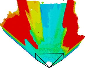
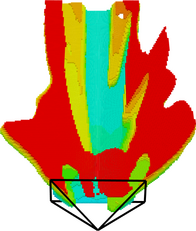
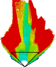
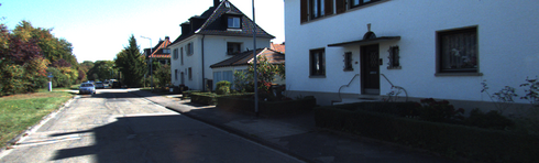
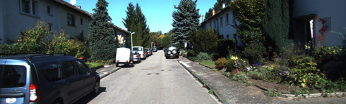
Figure 9: Voxelized reconstructions on SemanticKITTI (val set).

Input	Method	3D mesh	Novel depth			Novel view
			$+1$m, $0^{\circ}$	$+3$m, ${-}10^{\circ}$	${+}5$m, ${+}10^{\circ}$	${+}5$m, ${+}10^{\circ}$
	PixelNeRF
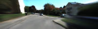
	MINE
	VisionNeRF
	SceneRF
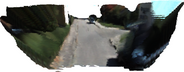
gray!50	PixelNeRF
	MINE
	VisionNeRF
	SceneRF
gray!50	PixelNeRF
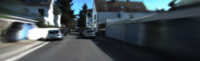
	MINE
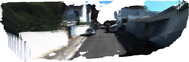
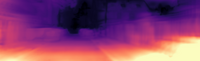
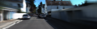
	VisionNeRF
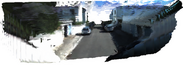
	SceneRF
gray!50	PixelNeRF
	MINE
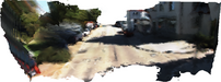
	VisionNeRF
	SceneRF
gray!50

Figure 10: Additional qualitative results on SemanticKITTI [4] (val.).

Input	Method	3D mesh	Novel depth			Novel view
			$+1$m, $0^{\circ}$	$+3$m, ${-}10^{\circ}$	${+}5$m, ${+}10^{\circ}$	${+}5$m, ${+}10^{\circ}$
	PixelNeRF
	MINE
	VisionNeRF
	SceneRF
gray!50	PixelNeRF
	MINE
	VisionNeRF
	SceneRF
gray!50	PixelNeRF
	MINE
	VisionNeRF
	SceneRF
gray!50	PixelNeRF
	MINE
	VisionNeRF
	SceneRF
gray!50

Figure 11: Additional qualitative results on SemanticKITTI [4] (val.).

Input	Method	3D mesh (w/ our recons. scheme)	Novel depth			Novel view
			$+0.2$m, $0^{\circ}$	$+0.2$m, ${-}20^{\circ}$	${+}0.4$m, ${+}20^{\circ}$	${+}0.4$m, ${+}20^{\circ}$
	PixelNeRF
	MINE
	VisionNeRF
	SceneRF
gray!50	PixelNeRF
	MINE
	VisionNeRF
	SceneRF
gray!50	PixelNeRF
	MINE
	VisionNeRF
	SceneRF

Figure 12: Additional qualitative results on BundleFusion [13] (val.).

Input	3D mesh	Novel depth			Novel view
		$+1$m, $0^{\circ}$	$+3$m, ${-}10^{\circ}$	${+}5$m, ${+}10^{\circ}$	${+}5$m, ${+}10^{\circ}$

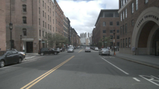
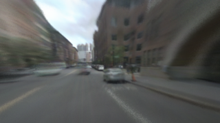
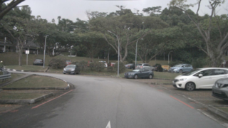
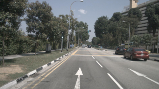
Figure 13: Additional generalization results on nuScenes [6]. The model is trained only on SemanticKITTI [4].

References

- [1] Panos Achlioptas, Olga Diamanti, Ioannis Mitliagkas, and Leonidas Guibas. Learning representations and generative models for 3D point clouds. In ICML, 2018.
- [2] Fatiha Anouar, Fouad Badran, and Sylvie Thiria. Probabilistic self-organizing map and radial basis function networks. Neurocomputing, 1998.
- [3] Jonathan T. Barron, Ben Mildenhall, Dor Verbin, Pratul P. Srinivasan, and Peter Hedman. Mip-nerf 360: Unbounded anti-aliased neural radiance fields. In CVPR, 2022.
- [4] J. Behley, M. Garbade, A. Milioto, J. Quenzel, S. Behnke, C. Stachniss, and J. Gall. SemanticKITTI: A Dataset for Semantic Scene Understanding of LiDAR Sequences. In ICCV, 2019.
- [5] Shariq Farooq Bhat, Ibraheem Alhashim, and Peter Wonka. AdaBins: Depth estimation using adaptive bins. In CVPR, 2021.
- [6] Holger Caesar, Varun Bankiti, Alex H. Lang, Sourabh Vora, Venice Erin Liong, Qiang Xu, Anush Krishnan, Yu Pan, Giancarlo Baldan, and Oscar Beijbom. nuscenes: A multimodal dataset for autonomous driving. In CVPR, 2020.
- [7] Ang Cao, C. Rockwell, and Justin Johnson. Fwd: Real-time novel view synthesis with forward warping and depth. In CVPR, 2022.
- [8] Anh-Quan Cao and Raoul de Charette. Monoscene: Monocular 3d semantic scene completion. In CVPR, 2022.
- [9] Xiaokang Chen, Kwan-Yee Lin, Chen Qian, Gang Zeng, and Hongsheng Li. 3d sketch-aware semantic scene completion via semi-supervised structure prior. In CVPR, 2020.
- [10] Zhiqin Chen, Andrea Tagliasacchi, and Hao Zhang. Bsp-net: Generating compact meshes via binary space partitioning. In CVPR, 2020.
- [11] Brian Curless and Marc Levoy. A volumetric method for building complex models from range images. In SIGGRAPH, 1996.
- [12] Manuel Dahnert, Ji Hou, Matthias Nießner, and Angela Dai. Panoptic 3d scene reconstruction from a single rgb image. In NeurIPS, 2021.
- [13] Angela Dai, Matthias Nießner, Michael Zollöfer, Shahram Izadi, and Christian Theobalt. Bundlefusion: Real-time globally consistent 3d reconstruction using on-the-fly surface re-integration. ACM Transactions on Graphics 2017 (TOG), 2017.
- [14] Kangle Deng, Andrew Liu, Jun-Yan Zhu, and Deva Ramanan. Depth-supervised NeRF: Fewer views and faster training for free. In CVPR, 2022.
- [15] Shivam Duggal and Deepak Pathak. Topologically-aware deformation fields for single-view 3d reconstruction. In CVPR, 2022.
- [16] Sayna Ebrahimi, Angjoo Kanazawa, and Trevor Darrell. Differentiable gradient sampling for learning implicit 3d scene reconstructions from a single image. In ICLR, 2022.
- [17] Haoqiang Fan, Hao Su, and Leonidas J. Guibas. A point set generation network for 3d object reconstruction from a single image. In CVPR, 2017.
- [18] Andreas Geiger, Philip Lenz, and Raquel Urtasun. Are we ready for autonomous driving? the kitti vision benchmark suite. In CVPR, 2012.
- [19] Georgia Gkioxari, Jitendra Malik, and Justin Johnson. Mesh r-cnn. In ICCV, 2019.
- [20] Clément Godard, Oisin Mac Aodha, and Gabriel J. Brostow. Unsupervised monocular depth estimation with left-right consistency. In CVPR, 2017.
- [21] Clément Godard, Oisin Mac Aodha, Michael Firman, and Gabriel J. Brostow. Digging into self-supervised monocular depth prediction. In ICCV, 2019.
- [22] Alexander Grabner, Peter M Roth, and Vincent Lepetit. Location field descriptors: Single image 3d model retrieval in the wild. In 3DV, 2019.
- [23] Zhizhong Han, Chao Chen, Yu-Shen Liu, and Matthias Zwicker. Drwr: A differentiable renderer without rendering for unsupervised 3d structure learning from silhouette images. In ICML, 2020.
- [24] Youichi Horry, Ken-Ichi Anjyo, and Kiyoshi Arai. Tour into the picture: using a spidery mesh interface to make animation from a single image. In SIGGRAPH, 1997.
- [25] Tao Hu, Shu Liu, Yilun Chen, Tiancheng Shen, and Jiaya Jia. Efficientnerf efficient neural radiance fields. In CVPR, 2022.
- [26] Siyuan Huang, Siyuan Qi, Yixin Zhu, Yinxue Xiao, Yuanlu Xu, and Song-Chun Zhu. Holistic 3d scene parsing and reconstruction from a single rgb image. In ECCV, 2018.
- [27] Yuanhui Huang, Wenzhao Zheng, Yunpeng Zhang, Jie Zhou, and Jiwen Lu. Tri-perspective view for vision-based 3d semantic occupancy prediction. In CVPR, 2023.
- [28] Zixuan Huang, Stefan Stojanov, Anh Thai, Varun Jampani, and James M. Rehg. Planes vs. chairs: Category-guided 3d shape learning without any 3d cues. In ECCV, 2022.
- [29] Hamid Izadinia, Qi Shan, and Steven M. Seitz. Im2cad. In CVPR, 2017.
- [30] Wonbong Jang and Lourdes Agapito. Codenerf: Disentangled neural radiance fields for object categories. In ICCV, 2021.
- [31] Jan J Koenderink, Andrea J van Doorn, and Astrid ML Kappers. Depth relief. Perception, 1995.
- [32] Andreas Kurz, Thomas Neff, Zhaoyang Lv, Michael Zollhofer, and Markus Steinberger. Adanerf: Adaptive sampling for real-time rendering of neural radiance fields. In ECCV, 2022.
- [33] Chen-Yu Lee, Vijay Badrinarayanan, Tomasz Malisiewicz, and Andrew Rabinovich. Roomnet: End-to-end room layout estimation. In ICCV, 2017.
- [34] Jiaxin Li, Zijian Feng, Qi She, Henghui Ding, Changhu Wang, and Gim Hee Lee. Mine: Towards continuous depth mpi with nerf for novel view synthesis. In ICCV, 2021.
- [35] Jie Li, Kai Han, Peng Wang, Yu Liu, and Xia Yuan. Anisotropic convolutional networks for 3d semantic scene completion. In CVPR, 2020.
- [36] Xingyi Li, Chaoyi Hong, Yiran Wang, Zhiguo Cao, Ke Xian, and Guosheng Lin. Symmnerf: Learning to explore symmetry prior for single-view view synthesis. In ACCV, 2022.
- [37] Yiming Li, Zhiding Yu, Christopher Choy, Chaowei Xiao, Jose M Alvarez, Sanja Fidler, Chen Feng, and Anima Anandkumar. Voxformer: Sparse voxel transformer for camera-based 3d semantic scene completion. In CVPR, 2023.
- [38] Yiyi Liao, Simon Donné, and Andreas Geiger. Deep marching cubes: Learning explicit surface representations. In CVPR, 2018.
- [39] Kai-En Lin, Yen-Chen Lin, Wei-Sheng Lai, Tsung-Yi Lin, Yichang Shih, and Ravi Ramamoorthi. Vision transformer for nerf-based view synthesis from a single input image. In WACV, 2023.
- [40] Feng Liu and Xiaoming Liu. 2d gans meet unsupervised single-view 3d reconstruction. In ECCV, 2022.
- [41] William E Lorensen and Harvey E Cline. Marching cubes: A high resolution 3d surface construction algorithm. In SIGGRAPH, 1987.
- [42] Ilya Loshchilov and Frank Hutter. Decoupled weight decay regularization. In ICLR, 2019.
- [43] Ruihang Miao, Weizhou Liu, Mingrui Chen, Zheng Gong, Weixin Xu, Chen Hu, and Shuchang Zhou. Occdepth: A depth-aware method for 3d semantic scene completion. In CVPR, 2023.
- [44] Ben Mildenhall, Pratul P. Srinivasan, Rodrigo Ortiz-Cayon, Nima Khademi Kalantari, Ravi Ramamoorthi, Ren Ng, and Abhishek Kar. Local light field fusion: Practical view synthesis with prescriptive sampling guidelines. TOG, 2019.
- [45] Ben Mildenhall, Pratul P. Srinivasan, Matthew Tancik, Jonathan T. Barron, Ravi Ramamoorthi, and Ren Ng. Nerf: Representing scenes as neural radiance fields for view synthesis. In ECCV, 2020.
- [46] Yue Ming, Xuyang Meng, Chunxiao Fan, and Hui Yu. Deep learning for monocular depth estimation: A review. Neurocomputing, 2021.
- [47] Norman Müller, Andrea Simonelli, Lorenzo Porzi, Samuel Rota Bulò, Matthias Nießner, and Peter Kontschieder. Autorf: Learning 3d object radiance fields from single view observations. In CVPR, 2022.
- [48] Thomas Neff, Pascal Stadlbauer, Mathias Parger, Andreas Kurz, Joerg H. Mueller, Chakravarty R. Alla Chaitanya, Anton S. Kaplanyan, and Markus Steinberger. DONeRF: Towards Real-Time Rendering of Compact Neural Radiance Fields using Depth Oracle Networks. CGF, 2021.
- [49] Richard A. Newcombe, Shahram Izadi, Otmar Hilliges, David Molyneaux, David Kim, Andrew J. Davison, Pushmeet Kohli, Jamie Shotton, Steve Hodges, and Andrew W. Fitzgibbon. Kinectfusion: Real-time dense surface mapping and tracking. ISMAR, 2011.
- [50] Yinyu Nie, Xiaoguang Han, Shihui Guo, Yujian Zheng, Jian Chang, and Jian Jun Zhang. Total3dunderstanding: Joint layout, object pose and mesh reconstruction for indoor scenes from a single image. In CVPR, 2020.
- [51] Michael Niemeyer, Lars M. Mescheder, Michael Oechsle, and Andreas Geiger. Differentiable volumetric rendering: Learning implicit 3d representations without 3d supervision. In CVPR, 2020.
- [52] Simon Niklaus, Long Mai, Jimei Yang, and Feng Liu. 3D ken burns effect from a single image. TOG, 2019.
- [53] Jeong Joon Park, Peter Florence, Julian Straub, Richard A. Newcombe, and Steven Lovegrove. DeepSDF: Learning continuous signed distance functions for shape representation. In CVPR, 2019.
- [54] Songyou Peng, Michael Niemeyer, Lars M. Mescheder, Marc Pollefeys, and Andreas Geiger. Convolutional occupancy networks. In ECCV, 2020.
- [55] S. Popov, Pablo Bauszat, and V. Ferrari. Corenet: Coherent 3d scene reconstruction from a single rgb image. In ECCV, 2020.
- [56] Jeremy Reizenstein, Roman Shapovalov, Philipp Henzler, Luca Sbordone, Patrick Labatut, and David Novotny. Common objects in 3D: Large-scale learning and evaluation of real-life 3D category reconstruction. In ICCV, 2021.
- [57] Konstantinos Rematas, Andrew Liu, Pratul P. Srinivasan, Jonathan T. Barron, Andrea Tagliasacchi, Tom Funkhouser, and Vittorio Ferrari. Urban radiance fields. In CVPR, 2022.
- [58] Konstantinos Rematas, Ricardo Martin-Brualla, and Vittorio Ferrari. Sharf: Shape-conditioned radiance fields from a single view. In ICML, 2021.
- [59] Barbara Roessle, Jonathan T. Barron, Ben Mildenhall, Pratul P. Srinivasan, and Matthias Nießner. Dense depth priors for neural radiance fields from sparse input views. In CVPR, 2022.
- [60] Luis Roldão, Raoul de Charette, and Anne Verroust-Blondet. Lmscnet: Lightweight multiscale 3d semantic completion. In 3DV, 2020.
- [61] Luis Roldao, Raoul De Charette, and Anne Verroust-Blondet. 3d semantic scene completion: a survey. IJCV, 2022.
- [62] David Salomon. Transformations and projections in computer graphics. Springer, 2006.
- [63] Prafull Sharma, Ayush Tewari, Yilun Du, Sergey Zakharov, Rares Ambrus, Adrien Gaidon, William T Freeman, Fredo Durand, Joshua B Tenenbaum, and Vincent Sitzmann. Seeing 3d objects in a single image via self-supervised static-dynamic disentanglement. arXiv preprint arXiv:2207.11232, 2022.
- [64] Vincent Sitzmann, Semon Rezchikov, William T. Freeman, Joshua B. Tenenbaum, and Fredo Durand. Light field networks: Neural scene representations with single-evaluation rendering. In NeurIPS, 2021.
- [65] Vincent Sitzmann, Michael Zollhöfer, and Gordon Wetzstein. Scene representation networks: Continuous 3d-structure-aware neural scene representations. In NeurIPS, 2019.
- [66] Peter Sturm and Steve Maybank. A method for interactive 3d reconstruction of piecewise planar objects from single images. In BMVC, 1999.
- [67] Cheng Sun, Chi-Wei Hsiao, Min Sun, and Hwann-Tzong Chen. Horizonnet: Learning room layout with 1d representation and pano stretch data augmentation. In CVPR, 2019.
- [68] Roman Suvorov, Elizaveta Logacheva, Anton Mashikhin, Anastasia Remizova, Arsenii Ashukha, Aleksei Silvestrov, Naejin Kong, Harshith Goka, Kiwoong Park, and Victor S. Lempitsky. Resolution-robust large mask inpainting with fourier convolutions. In WACV, 2021.
- [69] Mingxing Tan and Quoc Le. EfficientNet: Rethinking model scaling for convolutional neural networks. In ICML, 2019.
- [70] Maxim Tatarchenko, Alexey Dosovitskiy, and Thomas Brox. Single-view to multi-view: Reconstructing unseen views with a convolutional network. CoRR, 2015.
- [71] Alex Trevithick and Bo Yang. GRF: Learning a general radiance field for 3D scene representation and rendering. In ICCV, 2021.
- [72] Frank A Van den Heuvel. 3d reconstruction from a single image using geometric constraints. ISPRS, 1998.
- [73] Nanyang Wang, Yinda Zhang, Zhuwen Li, Yanwei Fu, Wei Liu, and Yu-Gang Jiang. Pixel2mesh: Generating 3d mesh models from single rgb images. In ECCV, 2018.
- [74] Zhou Wang, A.C. Bovik, H.R. Sheikh, and E.P. Simoncelli. Image quality assessment: from error visibility to structural similarity. TIP, 2004.
- [75] Olivia Wiles, Georgia Gkioxari, Richard Szeliski, and Justin Johnson. SynSin: End-to-end view synthesis from a single image. In CVPR, 2020.
- [76] Felix Wimbauer, Nan Yang, Christian Rupprecht, and Daniel Cremers. Behind the scenes: Density fields for single view reconstruction. In CVPR, 2023.
- [77] Haozhe Xie, Hongxun Yao, Shengping Zhang, Shangchen Zhou, and Wenxiu Sun. Pix2vox++: Multi-scale context-aware 3d object reconstruction from single and multiple images. IJCV, 2020.
- [78] Yiheng Xie, Towaki Takikawa, Shunsuke Saito, Or Litany, Shiqin Yan, Numair Khan, Federico Tombari, James Tompkin, Vincent Sitzmann, and Srinath Sridhar. Neural fields in visual computing and beyond. In EUROGRAPHICS, 2022.
- [79] Qiangeng Xu, Weiyue Wang, Duygu Ceylan, Radomir Mech, and Ulrich Neumann. Disn: Deep implicit surface network for high-quality single-view 3d reconstruction. In NeurIPS, 2019.
- [80] Guandao Yang, Xun Huang, Zekun Hao, Ming-Yu Liu, Serge Belongie, and Bharath Hariharan. Pointflow: 3d point cloud generation with continuous normalizing flows. In ICCV, 2019.
- [81] Alex Yu, Vickie Ye, Matthew Tancik, and Angjoo Kanazawa. pixelNeRF: Neural radiance fields from one or few images. In CVPR, 2021.
- [82] Sergey Zakharov, Rares Ambrus, Vitor Campagholo Guizilini, Dennis Park, Wadim Kehl, Frédo Durand, Joshua B. Tenenbaum, Vincent Sitzmann, Jiajun Wu, and Adrien Gaidon. Single-shot scene reconstruction. In CoRL, 2021.
- [83] Andy Zeng, Shuran Song, Matthias Nießner, Matthew Fisher, Jianxiong Xiao, and Thomas Funkhouser. 3dmatch: Learning local geometric descriptors from rgb-d reconstructions. In CVPR, 2017.
- [84] M. Zerroug and R. Nevatia. Part-based 3d descriptions of complex objects from a single image. TPAMI, 1999.
- [85] Cheng Zhang, Zhaopeng Cui, Yinda Zhang, Bing Zeng, Marc Pollefeys, and Shuaicheng Liu. Holistic 3d scene understanding from a single image with implicit representation. In CVPR, 2021.
- [86] Jason Y Zhang, Sam Pepose, Hanbyul Joo, Deva Ramanan, Jitendra Malik, and Angjoo Kanazawa. Perceiving 3d human-object spatial arrangements from a single image in the wild. In ECCV, 2020.
- [87] Richard Zhang, Phillip Isola, Alexei A. Efros, Eli Shechtman, and Oliver Wang. The unreasonable effectiveness of deep features as a perceptual metric. In CVPR, 2018.
- [88] Chuhang Zou, Alex Colburn, Qi Shan, and Derek Hoiem. Layoutnet: Reconstructing the 3d room layout from a single rgb image. In CVPR, 2018.
- [89] Nikola Zubi’c and Pietro Lio’. An effective loss function for generating 3d models from single 2d image without rendering. In AIAI, 2021.