The Multi-Cluster Fluctuating
Two-Ray Fading Model

Abstract

We introduce and characterize the Multi-cluster Fluctuating Two-Ray (MFTR) fading channel, generalizing both the fluctuating two-ray (FTR) and the $\kappa$-$\mu$ shadowed fading models through a more general yet equally mathematically tractable model. We derive all the chief probability functions of the MFTR model such as probability density function (PDF), cumulative distribution function (CDF), and moment generating function (MGF) in closed-form, having a mathematical complexity similar to other fading models in the state-of-the-art. We also provide two additional analytical formulations for the PDF and the CDF: (i) in terms of a continuous mixture of $\kappa$-$\mu$ shadowed distributions, and (ii) as an infinite discrete mixture of Gamma distributions. Such expressions enable to conduct performance analysis under MFTR fading by directly leveraging readily available results for the $\kappa$-$\mu$ shadowed or Nakagami-$m$ cases, respectively. We demonstrate that the MFTR fading model provides a much better fit than FTR and $\kappa$-$\mu$ shadowed models for small-scale measurements of channel amplitude in outdoor Terahertz (THz) wireless links. Finally, the performance of wireless communications systems undergoing MFTR fading is exemplified in terms of classical benchmarking metrics like the outage probability, both in exact and asymptotic forms, and the amount of fading.

I Introduction

As radio signals travel along a certain propagation environment, their interaction with objects, system agents and the propagation medium itself causes a number of effects that ultimately determine the amount of power being received at a given location. Classically, these phenomena have been well-characterized through the central limit theorem (CLT), that gives rise to a family of Gaussian models, being the most popular and widespread-used the Rayleigh/Rician models and also including more general ones like the Hoyt and Beckmann models [1, 2]. While CLT-based models have sufficed to characterize the effects of fading for decades, the rapid growth of wireless technologies along the $21^{\rm st}$ century requires more sophisticated efforts to properly capture the intrinsic nature of wireless propagation as we move up in frequency (where the CLT assumption may no longer hold) [3, 4], or when new use cases demand for improved accuracy, especially in highly low-outage regimes [5, 6].

The key advances in wireless fading channel modeling during the last years have been largely based on two different approaches. On the one hand, power envelope-based formulations were used by Yacoub to propose two families of generalized models: the $\kappa$-$\mu$ and the $\eta$-$\mu$ distributions [7]. These distributions were later generalized and unified through the $\kappa$-$\mu$ shadowed fading distribution [8, 9], which has become rather popular in the literature thanks to its ability to model a wide number of propagation conditions through a limited set of physically-justified parameters. On the other hand, ray-based formulations express the received signal as a superposition of a number of scattered waves with random phases [10]. Despite their clear physical motivation, the mathematical complexity associated to ray-based models grows when more than a few dominant waves are individually accounted for [11]. However, Durgin’s Two-Wave with Diffuse Power (TWDP) fading model and its subsequent generalizations [12, 13, 3] have also managed to become popular in the context of wireless channel modeling for higher-frequency bands. Specifically, the Fluctuating Two-Ray (FTR) fading model [3] has widely been adopted in mm-Wave environments, and even recently in terahertz (THz) bands [14].

Key to their success, the $\kappa$-$\mu$ shadowed and the FTR fading models share a number of features that are desirable for a stochastic fading model to be of practical use: (i) have a small number (three, in both cases) of physically justified parameters; (ii) have a reasonably good mathematical tractability; (iii) include simpler but popular fading models as special cases. However, because these two models arise from different physical formulations, they do not capture the same type of propagation behaviors. For instance, the FTR model has the ability to exhibit bimodality that often appears in field measurements [15, 16, 14], while the $\kappa$-$\mu$ shadowed one is inherently unimodal in its original formulation [8]. On the other hand, the $\kappa$-$\mu$ shadowed model can exhibit any sort of power-law asymptotic decay (diversity order), while ray-based models asymptotically decay with unitary slope [11].

Aiming to reconcile the two dominant approaches in the literature of stochastic fading channel modeling, which have hitherto evolved separately, we here introduce the Multi-cluster Fluctuating Two-Ray (MFTR) fading model. This newly proposed model is presented as the natural generalization and unification of both the FTR and the $\kappa$-$\mu$ shadowed fading models. Such generalization enables the presence of additional multipath clusters in the purely ray-based FTR model, and the consideration of two fluctuating specular components within one of the clusters, typically the first one received, of the $\kappa$-$\mu$ shadowed formulation. Despite being a generalization of the FTR and the $\kappa$-$\mu$ shadowed models, only one additional parameter is required over these baseline models. As we will later see, the MFTR model not only inherits the bimodality and asymptotic decay properties exhibited separately by the FTR and $\kappa$-$\mu$ shadowed models, respectively, but also brings out additional flexibility to model propagation features not captured by the models from which it is originated. The resulting formulations of the MFTR statistics are as tractable as those of the simpler baseline models, and of other fading models in the state-of-the-art. The key contributions of this work can be listed as follows:

• We derive the chief probability functions for the MFTR model, i.e., probability density function (PDF), cumulative distribution function (CDF), and moment generating function (MGF) in closed-form. These expressions allow for the computation of the MFTR statistics using special functions similar to those used in simpler, well-established fading models such as Rician shadowed [17], $\kappa$-$\mu$ shadowed [8], or FTR [3].

• Aiming to facilitate the use of the MFTR fading model for performance analysis purposes, we provide two alternative analytical formulations for the PDF and the CDF: one in terms of a continuous mixture of $\kappa$-$\mu$ shadowed distributions, and another one as an infinite discrete mixture of Gamma distributions. This allows to leverage the rich literature of performance analysis, so that existing results available either for the $\kappa$-$\mu$ shadowed or the Nakagami-$m$ cases can be used as a starting point to straightforwardly analyze the performance under MFTR fading.

• To experimentally validate the suitability of our model for experimental data, we carried out a fit of the MFTR model to small-scale fading field measurements in the terahertz (THz) band for outdoor line-of-sight (LOS) and non-line-of-sight (NLOS) environments.

• These results are used to analyze $i)$ the outage probability, $ii)$ the average bit error rate (BER), and $iii)$ the ergodic capacity (EC), under MFTR fading channels. The former two metrics are derived in exact and asymptotic form. Also, we study the impact of the model parameters on the amount of fading (AoF) metric.

The remainder of this paper is organized as follows: preliminaries and channel models are described in Section II. In Section III, analytical expressions are derived for the main statistics of the MFTR model. In section IV, we introduce the empirical validation of our fading model by fitting the MFTR model to a small-scale fading measurements campaign in outdoor THz wireless channels. Then, in Section V, performance analysis over MFTR fading channels is exemplified. Section VI shows illustrative numerical results and discussions. Finally, concluding remarks are provided in Section VII.

Notation: In what follows, $f_{(\cdot)}(\cdot)$ and $F_{(\cdot)}(\cdot)$ denote the PDF and CDF, respectively; $\mathbb{E}\left\{\cdot\right\}$ and $\mathbb{V}\left\{\cdot\right\}$ are the expectation and variance operators; $\Pr\left\{\cdot\right\}$ represents probability; $\lvert\cdot\rvert$ is the absolute value, $\simeq$ refers to “asymptotically equal to”, $\equiv$ reads as “is equivalent to”, $\approx$ denotes “approximately equal to” and $\sim$ refers to “statistically distributed as”. In addition, $\Gamma(\cdot)$ denotes the gamma function [18, Eq. (6.1.1)], $\gamma(\cdot,\cdot)$ is the lower incomplete gamma function [18, Eq. (6.5.2)], $\left(a\right)_{n}=\tfrac{\Gamma\left(a+n\right)}{\Gamma\left(a\right)}$ represents the Pochhammer’s symbol [18], $\mathbb{U}\left(\cdot,\cdot,\cdot\right)$ is the confluent hypergeometric Kummer function [19, Eq. (9.211)], ${}_{2}F_{1}\left(\cdot,\cdot;\cdot;\cdot\right)$ is the Gauss hypergeometric function [18, Eq. (15.1.1)], $P_{\alpha}(z)={}_{2}F_{1}\left(-\alpha,\alpha+1;1;\tfrac{1-z}{2}\right)$ is the Legendre function of the first kind of real degree $\alpha$ [18, Eq. (8.1.2)], $F_{D}^{(4)}\left(\cdot,\cdot,\cdot,\cdot,\cdot;\cdot;\cdot,\cdot,\cdot,\cdot\right)$ denotes the Lauricella hypergeometric function in four variables [20, Eq. (4), p. 33], $\Phi_{2}^{(4)}\left(\cdot,\cdot,\cdot,\cdot;\cdot;\cdot,\cdot,\cdot,\cdot\right)$ denotes the confluent hypergeometric function in four variables [20, Eq. (8), p. 34], and $\Phi_{2}\left(\cdot,\cdot;\cdot;\cdot,\cdot\right)$ is the bivariate confluent hypergeometric function [21, Eq. (4.19)].

II Preliminaries and Channel Models

According to [12], the small-scale random fluctuations of a radio signal transmitted over a wireless channel can be structured at the receiver as a superposition of $N$ waves arising from dominant (specular) components, plus a group of multipath waves associated to diffuse scattering. Therefore, under this model, the received complex baseband signal representing the wireless channel can be expressed as

$$V_{r}=\sum_{n=1}^{N}V_{n}\exp\left({j\phi_{n}}\right)+X_{1}+jY_{1},$$ (1)

where $V_{n}\exp(j\phi_{n})$ denotes the $n$th specular component with constant amplitude $V_{n}$ and uniformly distributed random phase $\phi_{n}\sim\mathcal{U}(0,2\pi)$. On the other hand, $X_{1}+jY_{1}$ is a circularly-symmetric complex Gaussian random variable (RV) with total power $2\sigma^{2}$, such that $X_{1},Y_{1}\sim\mathcal{N}(0,\sigma^{2})$, representing the scattering components associated to the NLOS propagation. This model allows to individually account for a number of dominant waves, together with the application of the CLT to the diffuse component, where a sufficiently large number of weak diffuse waves with independent phases is assumed.

The FTR channel model was proposed in [3] as a generalization of the TWDP model [12], where the latter arises when considering two dominant specular components (i.e., $N=2$) in (1). For its definition, the FTR model considers that the amplitudes of these two dominant components experience a joint fluctuation due to natural situations in different wireless scenarios (e.g., human body shadowing do to user motion, electromagnetic disturbances, and many others). Based on this, the complex signal under FTR fading can be formulated as [3]

$$V_{\rm{FTR}}=\sqrt{\zeta}V_{1}\exp\left({j\phi_{{1}}}\right)+\sqrt{\zeta}V_{2}\exp\left({j\phi_{2}}\right)+X_{1}+jY_{1},$$ (2)

where $\zeta$ is a unit-mean Gamma distributed RV whose PDF is given by

$$f_{\zeta}(x)=\frac{m^{m}x^{m-1}}{\Gamma(m)}\exp\left(-mx\right),$$ (3)

where $m$ denotes the shadowing severity index of the specular components. Note that when $m\rightarrow\infty$, then $\zeta$ degenerates into a deterministic value and the amplitudes of the two dominant specular components in (2) become constant. The FTR model in (2), besides fitting well with the field measurements in different wireless scenarios, also encompasses important statistical wireless channel models as particular cases. For instance, when no specular components are present in (2), i.e., $N=0$, the classical Rayleigh fading model arises. For a single LOS component, i.e., $N=1$, two fading models are obtained, namely, Rician and Rician shadowed [17] for constant and fluctuating amplitudes, respectively. Finally, for the case in which there are two dominant components (i.e., $N=2$) with constant amplitudes, (2) reduces to the TWDP fading model, also referred to as the Generalized Two-Ray fading model with uniformly distributed phases (GTR-U) [13].

On the other hand, power-envelope based formulations as those originally proposed by Yacoub [7] are defined from a different approach. Specifically, the squared amplitude (or instantaneous received power) of the $\kappa$-$\mu$ shadowed fading model is expressed as [8]

$$R^{2}=\sum_{i=1}^{\mu}|Z_{i}+\sqrt{\zeta}p_{i}|^{2},$$ (4)

where $\mu$ wave clusters are defined, the complex variables $Z_{i}$ denote the diffuse components associated to each cluster, $\zeta$ is a unit-mean Gamma distributed RV, as given in (3), and $p_{i}$ are complex amplitudes for the dominant components within each cluster. Notice that the FTR model in (2) can be physically interpreted as a single cluster in which both the specular and the diffuse components are part of the same cluster structure. With this in mind, we can combine a power-envelope definition as the one in (4) with the ray-based structure in (2) as follows.

As in [7], we consider a wireless signal composed of clusters of waves propagating in a non-homogeneous environment. Within each cluster, the scattered waves have random phases and similar delay times, while the intercluster delay-time spreads are assumed to be relatively large. All clusters of the multipath waves are assumed to have scattered waves with identical powers. Now, in the first cluster (which typically represents the first one arriving), two dominant specular components with random phases and arbitrary power are considered, as in (2), whereas in the rest of the clusters a specular component may also be present. Similarly to the models in [3] and [8], a dominant components are subject to the same source of random fluctuations. Under this channel model, the squared amplitude of the received signal is expressed as

$$R^{2}=\lvert\underset{\rm{cluster\ 1:}V_{\rm{FTR}}}{\underbrace{\sqrt{\zeta}\left(V_{1}e^{j\phi_{1}}+V_{2}e^{j\phi_{2}}\right)+Z_{1}}}\rvert^{2}+\underset{\rm{{\color[rgb]{0,0,0}additional\ clusters}}}{\underbrace{\sum_{i=2}^{\mu}\lvert\sqrt{\zeta}U_{i}e^{j\varphi_{i}}+Z_{i}\rvert^{2}},}$$ (5)

where $Z_{i}=X_{i}+jY_{i}$, for $i=\left\{1,\ldots,\mu\right\}$ in which $X_{i}$ and $Y_{i}$ are mutually independent zero-mean Gaussian processes with $\sigma^{2}$ variance, i.e., $\mathbb{E}\{X_{i}^{2}\}=\mathbb{E}\{Y_{i}^{2}\}=\sigma^{2}$. In cluster 1, the complex RVs represented by $V_{n}\exp(j\phi_{n})$, for $n=\left\{1,2\right\}$ denote the dominant specular components of the first arriving cluster, whereas $U_{i}\exp(j\varphi_{i})$ denotes the specular component of the $i$th cluster with constant amplitude $U_{i}$ and uniformly distributed random phase $\varphi_{i}\sim\mathcal{U}(0,2\pi)$. All the clusters are subject to the same source of random fluctuations as in the FTR and $\kappa$-$\mu$ shadowed models, denoted by the normalized RV $\zeta$. For the model in (5), we coin the name multicluster FTR (MFTR) model, to indicate the presence of additional multipath clusters in the original FTR model.

Because of the way it has been defined, the MFTR model defined in (5) includes both the FTR and the $\kappa$-$\mu$ shadowed models as special cases, which have independently been validated, empirically matching different wireless scenarios [3, 8], which guarantees the practical usefulness of the proposed model.

As in [7, 8], even though the cluster number $\mu$ is inherently a natural number, the MFTR model admits a generalization for $\mu\in\mathbb{R}^{+}$, which is considered in the subsequent derivations.

III Statistical Characterization of the MFTR Fading Model

In this section, the key first-order statistics of the newly proposed MFTR model are derived: the MGF, PDF and CDF. In the following derivations, let us consider the received power signal of the MFTR model, i.e., $W=R^{2}$, which from (5) can be rewritten as

$$W ={{\left(\sqrt{\zeta}\left({{V}_{1}}\cos{{\phi}_{1}}+{{V}_{2}}\cos{{\phi}_{2}}\right)+{{X}_{1}}\right)}^{2}}$$

$$+{{\left(\sqrt{\zeta}\left({{V}_{1}}\sin{{\phi}_{1}}+{{V}_{2}}\sin{{\phi}_{2}}\right)+{{Y}_{1}}\right)}^{2}}$$

$$+{\sum_{i=2}^{\mu}\left[\left({\sqrt{\zeta}U_{i}\cos\varphi_{i}+X_{i}}\right)^{2}+\left({\sqrt{\zeta}U_{i}sen\varphi_{i}+Y_{i}}\right)^{2}\right].}$$ (6)

As in [3], the MFTR model can be conveniently expressed by introducing the parameters $K$ and $\Delta$, which are respectively defined as

$$K=\frac{V_{1}^{2}+V_{2}^{2}+\sum\limits_{i=2}^{\mu}U^{2}_{i}}{2{{\sigma}^{2}}\mu},$$ (7)

$$\Delta=\frac{2{{V}_{1}}{{V}_{2}}}{V_{1}^{2}+V_{2}^{2}+\sum\limits_{i=2}^{\mu}U^{2}_{i}}.$$ (8)

The MFTR fading model is univocally defined by four shape parameters: $\{K,m,\mu\}\in\mathbb{R}^{+}$ and $\Delta\in[0,1]$. Similar to the interpretation of the Rician $K$ factor, $K$ represents the ratio of the average power of the specular components to the power of the remaining scattered components. On the other hand, the $\Delta$ parameter ranging from 0 to 1 shows how similar to each other are the average received powers of the dominant components in cluster 1 and how much power is allocated to the specular components of the rest of the clusters. Thus, when only one specular component is present in cluster 1 ($V_{1}$ or $V_{2}=0$) then $\Delta=0$, and the MFTR model collapses to the $\kappa$-$\mu$ shadowed model. When the magnitudes of the two specular components of the first cluster are equal ($V_{1}=V_{2}$) and the remaining clusters lack specular components ($U_{i}=0$ for $i=\left\{2,\ldots,\mu\right\}$) then $\Delta=1$. Furthermore, notice that for $\mu=1$ the MFTR model yields the FTR fading model and the definitions of $K$ and $\Delta$ of both models coincide.

Next, we introduce the distribution of the received power signal (or equivalently the instantaneous signal-to-noise ratio (SNR) when the noise comes into play) of the MFTR fading model. It is worth mentioning that the statistical characterization of the instantaneous received SNR, here denoted by $\gamma$, plays a pivotal role in designing or evaluating the performance of many practical wireless systems. Let $\gamma\triangleq(E_{s}/N_{0})W$ be the instantaneous received SNR through the MFTR fading channel, with $E_{s}$ and $N_{0}$ representing, respectively, the energy density per symbol and the power spectral density. Mathematically speaking, from (III), $\overline{\gamma}$ can be formulated as

$$\overline{\gamma}= \frac{E_{s}}{N_{0}}\mathbb{E}\left\{W\right\}$$

$${=\frac{E_{s}}{N_{0}}\Biggr{(}\mathbb{E}\left\{\lvert{\sqrt{\zeta}\left(V_{1}e^{j\phi_{1}}+V_{2}e^{j\phi_{2}}\right)+X_{1}+jY_{1}}\rvert^{2}\right\}}$$

$${+\sum_{i=2}^{\mu}\mathbb{E}\left\{\lvert\sqrt{\zeta}U_{i}e^{j\varphi_{i}}+X_{i}+jY_{i}\rvert^{2}\right\}\Biggr{)}}$$

$$= {\frac{E_{s}}{N_{0}}\left(V_{1}^{2}+V_{2}^{2}+2\sigma^{2}+\sum_{i=2}^{\mu}\left(U^{2}_{i}+2\sigma^{2}\right)\right)}$$

$$= \frac{E_{s}}{N_{0}}\left(V_{1}^{2}+V_{2}^{2}+\sum_{i=2}^{\mu}U^{2}_{i}+2\sigma^{2}\mu\right)$$

$${\stackrel{{\scriptstyle(a)}}{{=}}} \frac{E_{s}}{N_{0}}2\sigma^{2}\mu(1+K).$$ (9)

where in step (a), we employ (7) with the respective substitutions. With the aid of the previous definitions, the chief probability functions concerning the MFTR channel model can be derived as follows.

III-A MGF

In the first Lemma, presented below, we obtain a closed-form expression for the MGF.

Lemma 1.

The MGF of the instantaneous received SNR $\gamma$ under MFTR fading can be expressed as

$${{{\mathcal{M}}}_{\gamma}}\left(s\right)= \frac{{{m}^{m}}{{\mu}^{\mu}}{{\left(1+K\right)}^{\mu}}{{\left(\mu\left(1+K\right)-\overline{\gamma}s\right)}^{m-\mu}}}{{{\left(\sqrt{\mathcal{R}(\mu,m,K,\Delta;s)}\right)}^{m}}}$$

$$\times{{P}_{m-1}}\left(\frac{m\mu\left(1+K\right)-\left(\mu K+m\right)\overline{\gamma}s}{\sqrt{\mathcal{R}(\mu,m,K,\Delta;s)}}\right)$$ (10)

where $\mathcal{R}(\mu,m,K,\Delta;s)$ is a polynomial in $s$ given by

$$\mathcal{R}(\mu,m,K,\Delta;s) =\left[{{\left(m+\mu K\right)}^{2}}-{{\left(\mu K\Delta\right)}^{2}}\right]{{\overline{\gamma}}^{2}}{{s}^{2}}-2m\mu$$

$$\times\left(1+K\right)\left(m+\mu K\right)\overline{\gamma}s+{{\left[\left(1+K\right)m\mu\right]}^{2}}.$$ (11)

Proof.

See Appendix A. ∎

Note that the result in Lemma 1 is valid for any positive real value of $m$.

III-B PDF and CDF

Here, we derive the PDF and CDF of the SNR of the MFTR model. Even though these can be computed by performing a numerical Laplace inverse transform over the MGF in Lemma 1 for any arbitrary set of values of the shape parameters [1], it is possible to obtain closed-form expressions by assuming that the fading parameter $m$ takes integer values. For this purpose, we take advantage of the fact that, for $m\in\mathbb{Z}^{+}$, the Legendre function in the MGF obtained in (1) has an integer degree; thus, such Legendre function becomes a Legendre polynomial. The Legendre polynomial of an integer degree $n$ can be formulated as in [18, Eq. (22.3.8)] by

$$P_{n}(z)=\frac{1}{2^{n}}\sum_{q=0}^{\left\lfloor n/2\right\rfloor}(-1)^{n}C_{q}^{n}z^{n-2q},$$ (12)

where the $C_{q}^{n}$ term is expressed as

$$C_{q}^{n}=\binom{n}{q}\binom{2n-2q}{n}=\frac{\left(2n-2q\right)!}{q!(n-q)!(n-2q)!}.$$ (13)

From the MGF in (1) and with the help of (12), the closed-form expressions for the PDF and CDF of the RV $\gamma$ are obtained in the following Lemma.

Lemma 2.

Assuming that $m\in\mathbb{Z}^{+}$, the PDF and CDF of the SNR under MFTR fading can be formulated as (III-C) and (III-C), respectively.

Proof.

See Appendix B-A. ∎

The chief statistics of the MFTR fading model in (III-C) and (III-C) are given in terms of the multi-variate confluent hypergeometric function $\Phi_{2}^{(4)}\left(\cdot\right)$, which is rather common in well-established fading models such as Rician shadowed [17], $\kappa$-$\mu$ shadowed [8], or FTR [3]. Moreover, the computation of this function can be performed by resorting to an inverse Laplace transform as described in [1, Appendix 9B], and whose implementation in a simple and efficient way through MATLAB is given in [22]. Therefore, the evaluation of MFTR probability distributions does not pose any additional challenge compared to other well-known fading models in the state-of-the-art.

III-C Alternative formulations

Expressions in Lemmas 1 and 2 provide a complete formulation for the MFTR, equivalent in complexity to those originally proposed in [3] and [8] for the baseline FTR and $\kappa$-$\mu$ shadowed fading distributions, respectively. However, aiming to provide additional flexibility to the newly proposed MFTR model, as well as to facilitate its use for performance evaluation purposes, we now provide two alternative formulations for the PDF and CDF of the MFTR model.

We first propose a formulation of the MFTR model as a continuous mixture of $\kappa$-$\mu$ shadowed distributions. Secondly, we propose a formulation of the MFTR model as an infinite discrete mixture of Gamma distributions. These formulations are provided in the following two lemmas, and are valid for the entire range of values of the shape parameters $\kappa,\mu,m$ and $\Delta$.

$$f_{\gamma}(x)= \frac{\left(1+K\right)^{\mu}\mu^{\mu}}{2^{m-1}\Gamma(\mu)\overline{\gamma}^{\mu}}\left(\frac{m}{\sqrt{\left(m+\mu K\right)^{2}-\mu^{2}K^{2}\Delta^{2}}}\right)^{m}\sum_{q=0}^{\left\lfloor\frac{m-1}{2}\right\rfloor}\left(-1\right)^{q}C_{q}^{m-1}\left(\frac{m+\mu K}{\sqrt{\left(m+\mu K\right)^{2}-\mu^{2}K^{2}\Delta^{2}}}\right)^{m-1-2q}$$

$$\times \ x^{\mu-1}\Phi_{2}^{(4)}\Biggl{(}1+2q-m,m-q-1/2,m-q-1/2,\mu-m;\mu;-\frac{\left(1+K\right)m\mu}{\left(m+\mu K\right)\overline{\gamma}}x,-\frac{\left(1+K\right)m\mu}{\left(m+\mu K\left(1+\Delta\right)\right)\overline{\gamma}}x,$$

$$-\frac{\left(1+K\right)m\mu}{\left(m+\mu K\left(1-\Delta\right)\right)\overline{\gamma}}x,-\frac{\left(1+K\right)\mu}{\overline{\gamma}}x\Biggl{)}.$$ (14)

$$F_{\gamma}(x)= \frac{\left(1+K\right)^{\mu}\mu^{\mu}}{2^{m-1}\Gamma(\mu+1)\overline{\gamma}^{\mu}}\left(\frac{m}{\sqrt{\left(m+\mu K\right)^{2}-\mu^{2}K^{2}\Delta^{2}}}\right)^{m}\sum_{q=0}^{\left\lfloor\frac{m-1}{2}\right\rfloor}\left(-1\right)^{q}C_{q}^{m-1}\left(\frac{m+\mu K}{\sqrt{\left(m+\mu K\right)^{2}-\mu^{2}K^{2}\Delta^{2}}}\right)^{m-1-2q}$$

$$\times \ x^{\mu}\Phi_{2}^{(4)}\Biggl{(}1+2q-m,m-q-1/2,m-q-1/2,\mu-m;\mu+1;-\frac{\left(1+K\right)m\mu}{\left(m+\mu K\right)\overline{\gamma}}x,-\frac{\left(1+K\right)m\mu}{\left(m+\mu K\left(1+\Delta\right)\right)\overline{\gamma}}x,$$

$$-\frac{\left(1+K\right)m\mu}{\left(m+\mu K\left(1-\Delta\right)\right)\overline{\gamma}}x,-\frac{\left(1+K\right)\mu}{\overline{\gamma}}x\Biggl{)}.$$ (15)

Lemma 3.

When $m\in\mathbb{R}^{+}$, the PDF and CDF of the SNR of the MFTR distribution can be obtained by averaging the conditional $\kappa$-$\mu$ shadowed statistics over all possible realizations of $\theta$, as

$$f_{\gamma}(x)=\frac{1}{\pi}\int_{0}^{\pi}{{f}_{\gamma\left|\theta\right.}}(x)d\theta,$$ (16)

$$F_{\gamma}(x)=\frac{1}{\pi}\int_{0}^{\pi}{{F}_{\gamma\left|\theta\right.}}(x)d\theta,$$ (17)

where

$${{f}_{\gamma\left|\theta\right.}}(x)=\frac{{{\mu}^{\mu}}{{m}^{m}}{{\left(1+K\right)}^{\mu}}}{\Gamma(\mu)\overline{\gamma}{{\left(\mu K\left(1+\Delta\cos\theta\right)+m\right)}^{m}}}{{\left(\frac{x}{\overline{\gamma}}\right)}^{\mu-1}}$$

$$\times{{e}^{-\frac{\mu\left(1+K\right)}{\overline{\gamma}}x}}{{}_{1}}{{F}_{1}}\left(m;\mu;\frac{{{\mu}^{2}}K\left(1+\Delta\cos\theta\right)\left(1+K\right)}{\mu K\left(1+\Delta\cos\theta\right)+m}\frac{x}{\overline{\gamma}}\right){,}$$ (18)

$${{F}_{\gamma\left|\theta\right.}}(x)= \frac{{{\mu}^{\mu-1}}{{m}^{m}}{{\left(1+K\right)}^{\mu}}}{\Gamma(\mu){{\left(\mu K\left(1+\Delta\cos\theta\right)+m\right)}^{m}}}{{\left(\frac{x}{\overline{\gamma}}\right)}^{\mu}}\Phi_{2}\Bigl{(}\mu-m,$$

$$m;\mu+1;-\frac{\mu\left(1+K\right)x}{\overline{\gamma}},-\frac{\mu\left(1+K\right)}{\overline{\gamma}}$$

$$\times\frac{mx}{\mu K\left(1+\Delta\cos\theta\right)+m}\Bigl{)}.$$ (19)

Proof.

The conditional $\kappa$-$\mu$ shadowed PDF and CDF are obtained from [8, Eq. (4)] and [8, Eq. (6)] by substituting $\kappa$ and $\overline{\gamma}$ by (43) and (A), respectively. Then, using the relationships given in (A) and (48) that connect the $\kappa$-$\mu$ shadowed and MFTR models, (III-C) and (III-C) are obtained.∎

It must be noted that the Rician shadowed distribution is a particular case of the $\kappa$-$\mu$ shadowed distribution for the case when $\mu=1$. Thus, the integral connection between the FTR and the Rician shadowed distributions presented in [23], for arbitrary positive real $m$, is a particular case of Lemma 3 for $\mu=1$.

$$f_{\gamma}(x)=\sum_{i=0}^{\infty}{\color[rgb]{0,0,0}w_{i}}f_{X}^{\rm G}\left(\mu+i;\frac{\overline{\gamma}(\mu+i)}{\mu(K+1)};x\right).$$ (20)

$$F_{\gamma}(x)=\sum_{i=0}^{\infty}{\color[rgb]{0,0,0}w_{i}}F_{X}^{\rm G}\left(\mu+i;\frac{\overline{\gamma}(\mu+i)}{\mu(K+1)};x\right).$$ (21)

$${\color[rgb]{0,0,0}w_{i}=\frac{\Gamma(m+i)(\mu K)^{i}m^{m}}{\Gamma(m)\Gamma(i+1)}\frac{{\left({1-\Delta}\right)^{i}}}{{\sqrt{\pi}(\mu K(1-\Delta)+m)^{m+i}}}} {\color[rgb]{0,0,0}\sum_{q=0}^{i}\binom{i}{q}\frac{{\Gamma\left({q+\frac{1}{2}}\right)}}{{\Gamma\left({q+1}\right)}}\left({\frac{{2\Delta}}{{1-\Delta}}}\right)^{q}}$$

$${\color[rgb]{0,0,0}\times{}_{2}F_{1}\left({m+i,q+\frac{1}{2};q+1;\frac{{-2\mu K\Delta}}{{\mu K(1-\Delta)+m}}}\right),\quad m\in R^{+},}$$ (22)

$$f_{X}^{\rm G}\left(\lambda;\nu;y\right)=\frac{\lambda^{\lambda}}{\Gamma(\lambda)\nu^{\lambda}}y^{\lambda-1}\exp\left(-\frac{\lambda y}{\nu}\right),\quad F_{X}^{\rm G}\left(\lambda;\nu;y\right)=\frac{1}{\Gamma(\lambda)}\gamma\left(\lambda,\frac{\lambda y}{\nu}\right).$$ (23)

Lemma 4.

When $m\in\mathbb{R}^{+}$, the PDF and CDF of the SNR of the MFTR distribution can be obtained as an infinite discrete mixture of Gamma distributions. The corresponding expressions are given in equations (20) and (21), respectively, where $f_{X}^{\rm G}(\cdot)$ and $F_{X}^{\rm G}(\cdot)$ represent the PDF and CDF, respectively, of a Gamma distribution, which are both given in (23).

Proof.

See Appendix B-B. ∎

Here, we point out that the PDFs and CDFs in Lemmas 3 and 4 are valid for non-constrained fading values of the MFTR model. Expressions in Lemma 3, i.e., (16) and (17), are given in simple finite-integral form in terms of well-known functions in communication theory, where the integrands are continuous bounded functions and the integration interval is finite. Therefore, the evaluation of these integrals through numerical integration routines in commercial mathematical software packages poses no challenge, and in fact is an standard approach in communication theory – cfr. the proper integral forms of the Gaussian $Q$-function [24], or Simon and Alouini’s MGF approach to the performance analysis of wireless communication systems [1]. Expressions in Lemma 4, i.e., (20) and (21), are given as weighted sums of gamma distributions, which are a basic building block in many communication theory applications, and correspond to the case of assuming Nakagami-$m$ fading. These sets of expressions allow for leveraging the rich literature devoted to study baseline fading models like $\kappa$-$\mu$ shadowed and Nakagami-$m$, to directly evaluate the case of the more general MFTR model, when desired.

TABLE I: Conventional and generalized fading channel models derived from the MFTR distribution.

Fading Distribution	MFTR fading parameters
	$a)$ $\underline{\Delta}=0$, $\underline{K}\rightarrow\infty$, $\underline{m}=0.5$, $\underline{\mu}=1$
One-sided Gaussian	$b)$ $\underline{\Delta}=0$, $\underline{K}\rightarrow 0$, $\underline{m}\rightarrow\infty$, $\underline{\mu}=0.5$
	$c)$ $\underline{\Delta}=1$, $\underline{K}\rightarrow\infty$, $\underline{m}=1$, $\underline{\mu}=1$
	$a)$$\underline{\Delta}=0$, $\underline{K}\rightarrow\infty$, $\underline{m}=1$, $\underline{\mu}=1$
Rayleigh	$b)$ $\underline{\Delta}=0$, $\underline{K}\rightarrow 0$, $\underline{m}\rightarrow\infty$, $\underline{\mu}=1$
	$c)$ $\underline{\Delta}=0$, $\underline{K}=0$, $\forall\underline{m}$, $\underline{\mu}=1$
	$a)$ $\underline{\Delta}=0$, $\underline{K}=\tfrac{1-q^{2}}{2q^{2}}$, $\underline{m}=0.5$, $\underline{\mu}=1$
Nakagami-$q$ (Hoyt)	$b)$ $\forall\left\{\underline{\Delta},\underline{K}\right\}$, with $q=\sqrt{\tfrac{1+K(1-\Delta)}{1+K(1+\Delta)}}$,
	$\underline{m}=1$, $\underline{\mu}=1$
Nakagami-$m$	$a)$ $\underline{\Delta}=0$, $\underline{K}\rightarrow\infty$, $\underline{m}=m$, $\underline{\mu}=1$
	$b)$ $\underline{\Delta}=0$, $\underline{K}\rightarrow 0$, $\underline{m}\rightarrow\infty$, $\underline{\mu}=m$
Rician	$\underline{\Delta}=0$, $\underline{K}=K$, $\underline{m}\rightarrow\infty$, $\underline{\mu}=1$
Rician shadowed	$\underline{\Delta}=0$, $\underline{K}=K$, $\underline{m}=m$, $\underline{\mu}=1$
$\kappa$-$\mu$ shadowed	$\underline{\Delta}=0$, $\underline{K}=\kappa$, $\underline{m}=m$, $\underline{\mu}=\mu$
$\kappa$-$\mu$	$\underline{\Delta}=0$, $\underline{K}=\kappa$, $\underline{m}=\rightarrow\infty$, $\underline{\mu}=\mu$
$\eta$-$\mu$	$\underline{\Delta}=0$, $\underline{K}=(1-\eta)/(2\eta)$, $\underline{m}=\mu$, $\underline{\mu}=2\mu$
TWDP	$\underline{\Delta}=\Delta$, $\underline{K}=K$, $\underline{m}=\rightarrow\infty$, $\underline{\mu}=1$
Two-Wave	$\underline{\Delta}=\Delta$, $\underline{K}=\rightarrow\infty$, $\underline{m}=\rightarrow\infty$, $\underline{\mu}=1$
FTR	$\underline{\Delta}=\Delta$, $\underline{K}=K$, $\underline{m}=m$, $\underline{\mu}=1$
Fluctuating Two-Wave	$\underline{\Delta}=\Delta$, $\underline{K}=\rightarrow\infty$, $\underline{m}=m$, $\underline{\mu}=1$

\psfrag{A}[Bc][Bc][0.7]{\rm Case $\mathrm{A}$}\psfrag{B}[Bc][Bc][0.7]{\rm Case $\mathrm{B}$}\includegraphics[width=433.62pt]{./Figures/fig1mu.eps}

Figure 1: PDF of the MFTR signal envelope by varying $\mu$ in two different scenarios: Case $\mathrm{A}$: $\Delta=0.9$, $m=8$, $K=8$, $\overline{\gamma}=2$ and Case $\mathrm{B}$: $\Delta=0.9$, $m=4$, $K=15$, $\overline{\gamma}=1$.

\psfrag{H}[Bc][Bc][0.6]{$K_{\mathrm{dB}}^{\mathrm{B}}=25$ dB}\psfrag{Z}[Bc][Bc][0.6][0]{$K_{\mathrm{dB}}^{\mathrm{B}}=15$ dB}\includegraphics[width=433.62pt]{./Figures/fig2delta.eps}

Figure 2: PDF of the MFTR signal envelope for different values of $\Delta$, with $\mu=2$, $m=6$, $K=15$, and $\overline{\gamma}=1.5$. Markers correspond to MC simulations.

\psfrag{H}[Bc][Bc][0.6]{$K_{\mathrm{dB}}^{\mathrm{B}}=25$ dB}\psfrag{Z}[Bc][Bc][0.6][0]{$K_{\mathrm{dB}}^{\mathrm{B}}=15$ dB}\includegraphics[width=433.62pt]{./Figures/fig3m.eps}

Figure 3: PDF of the MFTR signal envelope for different values of $m$, with $\Delta=0.9$, $\mu=3$, $m=4$, $K=20$, and $\overline{\gamma}=1$. Markers correspond to MC simulations.

\psfrag{H}[Bc][Bc][0.6]{$K_{\mathrm{dB}}^{\mathrm{B}}=25$ dB}\psfrag{Z}[Bc][Bc][0.6][0]{$K_{\mathrm{dB}}^{\mathrm{B}}=15$ dB}\includegraphics[width=433.62pt]{./Figures/fig4K.eps}

Figure 4: PDF of the MFTR signal envelope for different values of $K$, with $m=5$, $\Delta=0.9$, $\mu=3$, and $\overline{\gamma}=1$. Markers correspond to MC simulations

III-D Special cases and effect of parameters

The MFTR model derived here is connected to other fading distributions commonly used in several wireless application scenarios, by specializing the corresponding set of parameters as stated in Table I. In order to avoid confusion, the parameters related to the MFTR distribution are underlined. We would like to mention that a multicluster version of the TWDP model in [12, 13] naturally appears as we let $m\rightarrow\infty$; however, this model alone has its own entity an deserves special attention as a separate item [25].

In Figs. 1-4, we illustrate how different propagation conditions affect the shape of the MFTR distribution, by evaluating the PDF of the received signal envelope $f_{R}(r)$ for a set of values of the shape parameters: $K$, $\Delta$, $m$ and $\mu$. The PDFs illustrated in the figures have been obtained by evaluating (III-C), although all mathematical expressions along this section have been double-checked through Monte Carlo (MC) simulations, which have been included with markers in the figures, whenever they don’t affect readability. Also, we also checked that the same results are obtained when eqs. (16) and (20) are used to evaluate the PDFs.

In Fig. 1, we clearly perceive that the MFTR model’s behavior is inherently bimodal (see Case $\mathrm{A}$). Interestingly, thanks to the presence of the $\mu$ parameter adequately combined with the other fading parameters, the MFTR model can exhibit a more pronounced bimodality as $\mu$ increases (see Case $\mathrm{B}$). Specifically, the MFTR model can exhibit both a left-bimodality (i.e., the first local maximum is larger) and a right-bimodality (i.e., the second local maximum is larger). This is in stark contrast with the behavior of the baseline $\kappa$-$\mu$ shadowed (unimodal) or FTR distributions (only right-bimodality) from which the MFTR distribution originates. This feature brings additional flexibility to improve the versatility of the MFTR model to fit field measurements in emerging wireless scenarios such as mm-Wave and sub-terahertz bands [14].

In Fig. 2, it is confirmed that for low values of $\Delta$, i.e., one specular component is dominant in cluster 1, the MFTR distribution exhibits a unimodal behavior similar to the $\kappa$-$\mu$ shadowed case. Conversely, for larger values of $\Delta$, i.e., two specular components with similar amplitudes are present in cluster 1 which dominate the power of the specular components of the remaining clusters, the MFTR distribution exhibits a bimodal behavior. From Figs. 3-4, we can see that such bimodality of the MFTR distribution is also closely linked to parameters $m$ and $K$. Specifically, large values of $m$ or $K$ yield a more pronounced bimodality. Conversely, low values of $m$ or $K$ tend to smoothen such bimodality.

(a)

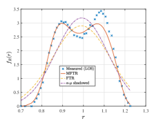
(b)

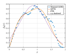
(c)

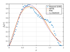
(d)

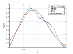
(e)

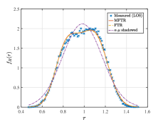
(f)

Figure 5: Empirical vs theoretical PDFs of the received signal amplitude for LOS and NLOS scenarios.

IV Empirical Validation

In this section, we validate the suitableness of the MFTR model to capture the stochastic features of outdoor THz wireless links in the 142 GHz band. For this purpose, we employ the empirical data presented in [26], in which sets of experimental measurements have been conducted on the campus of Aalto University in Finland by assuming LOS and NLOS scenarios. More details concerning the experimental setup can be found in [27]. Here, our goal is to assess the ability of the MFTR to capture the the physical behavior of the THz wireless link by means of multipath clusters in the presence of two dominant specular components with fluctuating amplitudes.

In order to quantify the fitting accuracy, we use the well-defined and widely-accepted mean-square-error (MSE) test. Specifically, the MSE measures the goodness of fit between the empirical and theoretical PDFs , denoted by $\widehat{f}_{R}(\cdot)$ and $f_{R}(\cdot)$, respectively, i.e.,

$$\text{MSE}=\frac{1}{T}\sum_{i=1}^{T}\left(\widehat{f}_{R}(r_{i})-f_{R}(r_{i})\right)^{2},$$ (24)

where $T$ denotes the number of empirical PDF values.

TABLE II: Fitting Results of MFTR, FTR and $\kappa$-$\mu$ shadowed fading models for different scenarios.

Case	Distribution	$K$	$\Delta$	$\mu$	$m$	MSE	Case	Distribution	$K$	$\Delta$	$\mu$	$m$	MSE
Fig. 5a	MFTR	10.788	0.29	39.991	90.252	0.06746	Fig. 5d	MFTR	10.558	0.850	0.827	4.356	0.00304
	FTR	38.141	0.003	1	79.323	0.32746		FTR	7.192	0.872	1	4.442	0.00306
	$\kappa$-$\mu$ shadowed	11.102	0	2.986	89.337	0.32772		$\kappa$-$\mu$ shadowed	4.820	0	0.645	2.288	0.00559
Fig. 5b	MFTR	4.225	0.999	1.055	38.868	0.00351	Fig. 5e	MFTR	20.717	0.403	3.108	84.333	0.00241
	FTR	4.113	0.993	1	89.999	0.00354		FTR	67.293	0.390	1	75.187	0.00276
	$\kappa$-$\mu$ shadowed	3.924	0	0.650	2.868	0.00791		$\kappa$-$\mu$ shadowed	24.834	0	0.598	73.775	0.02689
Fig. 5c	MFTR	3.284	0.999	1.267	5.481	0.00543	Fig. 5f	MFTR	17.938	0.596	0.400	79.519	0.00347
	FTR	1.958	1	1	18.909	0.00634		FTR	6.204	0.657	1	95.614	0.00362
	$\kappa$-$\mu$ shadowed	0.525	0	1.023	21.989	0.00710		$\kappa$-$\mu$ shadowed	39.995	0	0.107	78.744	0.00392

Table II reports the values of the MSE and the estimated fading parameters using the fminsearch function of the Optimization Toolbox of MATLAB for each target distribution. Bold-faced numbers highlight the best-fitting result in each scenario. Here, according to the MSE criteria, we can see that the MFRT fading channel model has achieved the best fittings in all scenarios under study. On the other hand, in Fig. 5, we compare the theoretical PDFs of MFTR, FTR, and $\kappa$-$\mu$ shadowed fading models against the THz channel measurements for LOS and NLOS environments described in [26, Fig. 1]. From all traces, it can be observed that the MFRT model yields a more accurate fit to the empirical distributions. This is in accordance with the MSE values shown in Table II. At this point, an important remark is in order. Firstly, we want by no means to provide a thorough and tedious comparison between the proposed MFTR model and existing fading models when applied to fit channel measurements in THz or millimeter bands. Instead, we mainly want to provide some evidence that, for selected channel measurement campaigns, the proposed MFTR fading model offers a good balance between versatility, flexibility, the goodness of fit and physical underpinnings. For instance, for the NLOS environment in Fig. 5a, the MFTR captures the richness of the dispersion through a high value of $\mu$ (i.e., $39.99$), which also allows capturing the pronounced bimodality of the distribution. Another key interpretation of this fading parameter is that as $\mu$ increases, the MFTR model smooths out the goodness of fit as the distribution moves away from the origin on the x-axis. In particular, this behavior is present in Figs. 5a and 5e, where the empirical distributions start at approximately $0.7$ and $0.5$ on the x-axis, respectively. Conversely, in all other figures, the empirical measurements begin at $0$ on the x-axis, which translates to small values of $\mu$. In short, the MFTR model provides additional flexibility (i.e., more degrees of freedom) to characterize small-scale empirical fading data compared to $\kappa$-$\mu$ shadowed and FTR models from which it originates.

V Performance Analysis in Wireless Systems

In this section, we illustrate the flexibility of the MFTR model when used for performance analysis. For exemplary purposes, we analyze key performance metrics such as the outage probability (OP), both in exact and asymptotic forms, as well as the AoF [1].

V-A Outage Probability

The instantaneous Shannon channel capacity per unit bandwidth is defined as

$$C=\log_{2}(1+\gamma).$$ (25)

The outage probability is defined as the probability that the capacity $C$ falls below a certain threshold rate $R_{\rm th}$, i.e.,

$$P_{\rm out} =\Pr\left\{C<R_{\rm th}\right\}=\Pr\left\{\log_{2}(1+\gamma)<R_{th}\right\}$$

$$=\Pr\left\{\gamma<\underbrace{2^{R_{\rm th}}-1}_{\gamma_{\rm th}}\right\}.$$ (26)

Consequently, the OP is given in terms of SNR’s CDF as

$$P_{\rm out} =F_{\gamma}\left(2^{R_{\rm th}}-1\right),$$ (27)

in which $F_{\gamma}\left(\cdot\right)$ is given by either (III-C), (21) or (17). Although expressed in exact form in terms of the MFTR CDFs previously derived, $P_{\rm out}$ provides a limited insight concerning the effect of fading parameters on the system performance. Thus, we introduce a closed-form asymptotic OP expression to evaluate the high-SNR regime’s system performance below.

V-B Asymptotic Outage Probability

Here, to get further insights about the role of the fading parameters on system performance, we derive an asymptotic expression to investigate the behavior of the OP given in (27) in the high-SNR regime. Our goal is to obtain an asymptotic expression in the form $P_{\rm out}\simeq\mathrm{G}_{c}\left(\gamma_{\rm th}/\overline{\gamma}\right)^{\mathrm{G}_{d}}$ [28], where $\mathrm{G}_{c}$ and $\mathrm{G}_{d}$ denote the power offset and the diversity order, respectively. Hence, the corresponding asymptotic OP is given in the following Proposition.

Proposition 1.

The asymptotic expression of the OP over MFTR channels can be obtained as

$$P_{\rm out}\simeq \frac{\mu^{\mu-1}(1+K)^{\mu}m^{m}(2^{R_{\rm th}}-1)^{\mu}}{\Gamma(\mu)\overline{\gamma}^{\mu}\left(m-\left(\Delta-1\right)K\mu\right)^{m}}$$

$$\times{}_{2}F_{1}\left(1/2,m;1;\frac{2\Delta K\mu}{K\mu\left(1-\Delta\right)+m}\right).$$ (28)

Proof.

See Appendix C-A. ∎

From (V-B), notice that the diversity order is linked to the number of multipath waves clusters, i.e., $\mathrm{G}_{d}=\mu$.

V-C Amount of Fading

The AoF is a popular metric used to quantify the severity of fading experienced during transmission under fading channels. It is defined as [1]

$$\rm{AoF}=\frac{\mathbb{V}\left\{\gamma\right\}}{\mathbb{E}\left\{\gamma\right\}^{2}}=\frac{\mathbb{E}\left\{\gamma^{2}\right\}-\mathbb{E}\left\{\gamma\right\}^{2}}{\mathbb{E}\left\{\gamma\right\}^{2}}=\frac{\mathbb{E}\left\{\gamma^{2}\right\}}{\mathbb{E}\left\{\gamma\right\}^{2}}-1.$$ (29)

Based on (29), a closed-form expression of the AoF is given as stated in the following Proposition.

Proposition 2.

Assuming non-constrained arbitrary fading values, a closed-form expression for the AoF over MFTR channels can be formulated as

$$\rm{AoF}= \left(1-\frac{K^{2}}{(1+K)^{2}}\right)\left(1+\frac{1}{\mu}\right)+\frac{K^{2}}{(1+K)^{2}}$$

$$\times\left(1+\frac{1}{m}\right)\left(1+\frac{\Delta^{2}}{2}\right)-1.$$ (30)

Proof.

See Appendix C-B. ∎

$$\overline{P_{e}}= \frac{\left(1+K\right)^{\mu}\mu^{\mu}}{2^{m-1}\Gamma(\mu+1)\overline{\gamma}^{\mu}}\left(\frac{m}{\sqrt{\left(m+\mu K\right)^{2}-\mu^{2}K^{2}\Delta^{2}}}\right)^{m}\sum_{q=0}^{\left\lfloor\frac{m-1}{2}\right\rfloor}\left(-1\right)^{q}C_{q}^{m-1}\left(\frac{m+\mu K}{\sqrt{\left(m+\mu K\right)^{2}-\mu^{2}K^{2}\Delta^{2}}}\right)^{m-1-2q}$$

$$\times \ \sum_{r=1}^{R}\alpha_{r}\frac{2^{\mu-1}}{\beta_{r}^{\mu}\sqrt{\pi}}\Gamma\left(\mu+1/2\right)F_{D}^{(4)}\Biggl{(}\mu+\frac{1}{2},1+2q-m,m-q-\frac{1}{2},m-q-\frac{1}{2},\mu-m;\mu+1;-\frac{2\left(1+K\right)m\mu}{\beta_{r}\left(m+\mu K\right)\overline{\gamma}},$$

$$-\frac{2\left(1+K\right)m\mu}{\beta_{r}\left(m+\mu K\left(1+\Delta\right)\right)\overline{\gamma}},-\frac{2\left(1+K\right)m\mu}{\beta_{r}\left(m+\mu K\left(1-\Delta\right)\right)\overline{\gamma}},-\frac{2\left(1+K\right)\mu}{\beta_{r}\overline{\gamma}}\Biggl{)}.$$ (31)

V-D Average BER

The exact solution for the average BER affected by additive white Gaussian noise (AWGN), over the output SNR can be defined as in [1] by

$$\overline{P_{e}}=\int_{0}^{\infty}P_{E}(x)f_{\gamma}(x)dx,$$ (32)

where $P_{E}(x)$ denotes the conditional error probability (CEP). Considering integration by parts in (32), the average BER can be computed as function of the CDF, given by

$$\overline{P_{e}}=-\int_{0}^{\infty}P_{E}^{{}^{\prime}}(x)F_{\gamma}(x)dx,$$ (33)

where $P_{E}^{{}^{\prime}}(x)$ denotes the first order derivative of the CEP. For several modulation schemes, $P_{E}(x)$ can be defined as in [1] by

$$P_{E}(x)=\sum_{r=1}^{R}\alpha_{r}Q\left(\sqrt{\beta_{r}x}\right),$$ (34)

where $\left\{\beta_{r},\alpha_{r}\right\}_{r=1}^{R}$ are constants that depend on the type of modulation. Taking the derivative of (34), it follows that

$$P_{E}^{{}^{\prime}}(x)=-\sum_{r=1}^{R}\alpha_{r}\sqrt{\frac{\beta_{r}}{8\pi x}}e^{-\frac{\beta_{r}x}{2}}.$$ (35)

Finally, by substituting (III-C) and (35) into (33) followed by some manipulations and then making use of [21,  Eq. (43)], a closed-form fashion of the average BER can be expressed as in (V-C).

V-E Asymptotic Average BER

In this section, we derive an asymptotic closed-form expression for the average BER in order to gain more insights into the impact of the fading parameters of the systems. Here, we consider the behavior in the high SNR regime where $\overline{\gamma}\rightarrow\infty$. Again, our aim is to express the asymptotic average BER as $\overline{P_{e}}^{\infty}\simeq\mathrm{G}_{c}\overline{\gamma}^{-\mathrm{G}_{d}}$ [28]. For that purpose, we use the approach in [28, Proposition 3], where asymptotic $\overline{P_{e}}$ can be obtained from the MGF given in (1). In light of this, we first compute $\lvert{{{\mathcal{M}}}_{\gamma}}\left(s\right)\rvert$ as

$$\lvert{{{\mathcal{M}}}_{\gamma}}\left(s\right)\rvert= \frac{{{m}^{m}}{{\mu}^{\mu}}{{\left(1+K\right)}^{\mu}}{{}}}{{{\left(\sqrt{\left(m+\mu K\right)^{2}-\left(\mu K\Delta\right)^{2}}\right)}^{m}}}$$

$$\times{{P}_{m-1}}\left(\frac{m\mu\left(1+K\right)}{\sqrt{\left(m+\mu K\right)^{2}-\left(\mu K\Delta\right)^{2}}}\right)\frac{\lvert s\rvert^{-1}}{\overline{\gamma}^{\mu}}$$

$$+o\left(\lvert s\rvert^{-1}\right),$$ (36)

where we write a function $a(x)$ of $x$ as $o(x)$ if $\lim_{x\to 0}a(x)/x=0$, in which the Legendre polynomial is computed from (12). Then, by carrying out the same methodology given in [28, Proposition 1 and 3], $\overline{P_{e}}^{\infty}$ can be defined as

$$\overline{P_{e}}^{\infty}\simeq \frac{{{m}^{m}}{{\mu}^{\mu}}{{\left(1+K\right)}^{\mu}}{{}}}{{{\left(\sqrt{\left(m+\mu K\right)^{2}-\left(\mu K\Delta\right)^{2}}\right)}^{m}}}\sum_{r=1}^{R}\alpha_{r}\frac{2^{\mu-1}}{\beta_{r}^{\mu}\sqrt{\pi}}\Gamma\left(\mu+\tfrac{1}{2}\right)$$

$$\times{{P}_{m-1}}\left(\frac{m\mu\left(1+K\right)}{\sqrt{\left(m+\mu K\right)^{2}-\left(\mu K\Delta\right)^{2}}}\right)\frac{1}{\overline{\gamma}^{\mu}}.$$ (37)

As in $P_{\rm out}$ metric, from (V-E), it is clearly seen that the diversity order of $\overline{P_{e}}$ is associated to the number of multipath waves clusters, i.e., $\mathrm{G}_{d}=\mu$.

V-F Ergodic Capacity

The EC is defined as the maximum achievable rate averaged over all the fading contributions. Mathematically speaking, the EC can be expressed as [1]

$$\overline{C}= \int_{0}^{\infty}\log_{2}\left(1+x\right)f_{\gamma}(x)dx,$$ (38)

where $f_{\gamma}(\cdot)$ is the PDF of the received SNR $\gamma$ under MFTR fading channels. For the sake of mathematical tractability, we employ the alternative PDF of the MFTR model given in terms of the mixture of Gamma Distributions to compute $\overline{C}$. Hence, substituting (20) into (38), and after some manipulations, EC can be obtained as

$$\overline{C}= \sum_{i=0}^{\infty}{w_{i}}\frac{\left(\frac{\lambda}{\nu}\right)^{\lambda}}{\Gamma(\lambda)\ln(2)}\sum_{k=1}^{\infty}\frac{1}{k}\Gamma(k+\lambda)\mathbb{U}\left(k+\lambda,1+\lambda,\frac{\lambda}{\nu}\right),$$ (39)

where $w_{i}$ is given by (III-C), $\lambda=\mu+i$, and $\nu=\frac{\overline{\gamma}(\mu+i)}{\mu(K+1)}$.

\psfrag{A}[Bc][Bc][0.7]{$\mathrm{\textit{m}=10}$}\psfrag{B}[Bc][Bc][0.7]{$\mathrm{\textit{m}=2}$}\includegraphics[width=433.62pt]{./Figures/OP1.eps}

Figure 6: $P_{\rm out}$ as a function of the average SNR, for different values of $\mu$ and $m$. The remaining fading parameters are: $K=15,\ \Delta=0.1,\ R_{\rm th}=1$. Solid lines correspond to the $P_{\rm out}$ derived from (27), and dotted lines correspond to the asymptotic $P_{\rm out}$ derived from (V-B). Markers denote MC simulations

VI Numerical Results

In this section, we provide illustrative numerical results along with MC simulations to verify the analytical performance metrics derived in the previous section by assuming different fading conditions.

Figs. 6 and. 7 illustrate the impact of different propagation mechanisms, namely, NLOS- LOS-condition, LOS fluctuation, the existence of one/two dominant components in cluster 1, and clustering of multipath waves, on the OP performance. In both figures, we assume $K=15$ and $R_{\rm th}=1$. Specifically, in Fig. 6, we evaluate the OP vs. the average SNR by varying $\mu$ and $m$ for $\Delta=0.1$. From all traces, it can be observed that a contribution of the LOS component with a mild fluctuation ($m=10$) together with a rich scattering environment ($\mu=3$) favors the OP performance. Conversely, when both the LOS fluctuation is severe (i.e., lower values of $m$), and a poor scattering condition exists ($\mu=1$), the OP performance is noticeably reduced. On the other hand, in Fig. 7, we show the OP as a function of the average SNR for different fading values of $\Delta$ and $\mu$, assuming a mild fluctuation ($m=5$) for the LOS component. Here, we can see that the combination of similar ($\Delta=0.9$) specular components with many clusters of multipath waves ($\mu=4$) derives into a better OP behavior. However, in the opposite scenario, i.e., dissimilar ($\Delta=0.1$) specular components together with reduced clustering of scattering waves, the OP significantly deteriorates.

\psfrag{A}[Bc][Bc][0.7]{$\Delta=0.1$}\psfrag{B}[Bc][Bc][0.7]{$\Delta=0.9$}\includegraphics[width=433.62pt]{./Figures/OP2.eps}

Figure 7: $P_{\rm out}$ as a function of the average SNR, for different values of $\mu$ and $\Delta$. The remaining parameters are: $K=15,\ m=5,\ R_{\rm th}=1$. Solid lines correspond to the $P_{\rm out}$ derived from (27), and dotted lines correspond to the asymptotic $P_{\rm out}$ derived from (V-B). Markers denote MC simulations

Furthermore, in Figs. 6 and. 7, we see that the number of clusters of multipath waves contributes directly to the OP slope. This means that the decay in the OP is steeper (i.e., better performance) as the number of scattering wave clusters increases. This is in coherence with the derived diversity order, i.e., $\mathrm{G}_{d}=\mu$.

Finally, Fig. 8 depicts the average BER for binary phase-shift keying (BPSK) modulation vs. the average SNR by varying $\mu$ and $\Delta$ for a fixed LOS fluctuation, i.e., $m=2$. The parameters for BPSK modulation in (V-C) are set to $R=1$, and $\left\{\beta_{r},\alpha_{r}\right\}_{r=1}^{R}=\left\{2,1\right\}$. From all curves, we can see that the eventual similarity specular components in the first cluster does not dominate ($\Delta=0.1$), experiencing a moderate fluctuation ($m=2$) in a rich scattering condition ($\mu=3$) yields the best $\overline{P_{e}}$ behavior. Conversely, average BER performance worsens as $\Delta$ increases coupled with a dispersion-poor environment. Also, as in the $P_{\rm out}$ metric, the $\overline{P_{e}}$ slope directly depends on the number of clusters of multipath waves, which is associated with the obtained diversity order $\mathrm{G}_{d}=\mu$.

VII Conclusions

We introduced, for the first time in the literature, a stochastic fading model that combines the key features of ray-based and power envelope-based approaches. This newly proposed fading model unifies and generalizes both the FTR and the $\kappa$-$\mu$ shadowed fading models, with a comparable mathematical complexity. The MFTR model captures, through a limited set of physically-meaningful parameters, a number of propagation conditions that appear in many practical scenarios: LOS/NLOS propagation, amplitude imbalances between dominant specular components, random fluctuation of the dominant specular waves, and clustering of multipath waves. In order to facilitate its use for performance analysis purposes, alternative expressions for its statistics are derived, which enable us to express the desired performance metric under MFTR fading directly from those available either for $\kappa$-$\mu$ shadowed or Nakagami-$m$ fading. All these features make the MFTR model a strong contender to being the most generalized and comprehensive fading channel model in the state-of-the-art up to the present date.

\psfrag{A}[Bc][Bc][0.7]{$\Delta=0.1$}\psfrag{B}[Bc][Bc][0.7]{$\Delta=0.9$}\includegraphics[width=433.62pt]{./Figures/FigureABER.eps}

Figure 8: $\overline{P_{e}}$ for BPSK modulation as a function of the average SNR, for different values of $\mu$ and $\Delta$. The remaining parameters are: $K=10,\ m=2$. Solid lines correspond to the $\overline{P_{e}}$ derived from (V-C), and dotted lines correspond to the asymptotic $\overline{P_{e}}^{\infty}$ derived from (V-E). Markers denote MC simulations.

Appendix A Proof of Lemma 1

Departing from a generalized physical cluster-based model [8, 7], let us consider a compact form expression for the signal power, $W$, as in (4), given by

$${W}=\sum_{i=1}^{\mu}\left|Z_{i}+\sqrt{\zeta}p_{i}\right|^{2}.$$ (40)

In purely cluster-based models, the total power of the dominant components can be distributed indistinctly throughout the clusters. Here, without loss of generality, we assume that two specular components are allocated to cluster 1, and each of the remaining clusters may include one specular component. With this in mind, the dominant specular component, denoted by $p_{i}$, of the $i$th cluster can be expressed as

$$p_{i}=\begin{cases}U_{i}e^{j\varphi_{i}},&\text{for $\forall{i}>1$}\\ V_{1}e^{j\phi_{1}}+V_{2}e^{j\phi_{2}}=e^{j\phi_{1}}\left(V_{1}+V_{2}e^{j\alpha}\right),&\text{for ${i}=1$},\end{cases}$$ (41)

where $\alpha=\phi_{2}-\phi_{1}$ is the phase difference between the specular components of cluster 1. Given that $\phi_{n}\sim\mathcal{U}(0,2\pi)$ and because of the modulo $2\pi$ operation, it follows that, $\alpha\sim\mathcal{U}(0,2\pi)$ [13].

Let us consider the channel model given in (40) conditioned to a particular realization $\alpha=\theta$ of the RV characterizing the phase difference between the two LOS components in cluster 1. Then, (40) can be seen as a $\kappa$-$\mu$ shadowed distributed RV for a given $\theta$, where $\lvert p_{1}\rvert$ is now constant (i.e., deterministic) and no longer arbitrarily distributed. Based on this, the mean power of the dominant components for the underlying $\kappa$-$\mu$ shadowed RV in (40), conditioned on $\theta$, i.e., $d_{\theta}^{2}\stackrel{{\scriptstyle\Delta}}{{=}}d^{2}|_{\alpha=\theta}$ is given by

$$d_{\theta}^{2}= \sum^{\mu}_{i=1}\lvert p_{i}\rvert^{2}=\lvert V_{1}+V_{2}e^{j\theta}\rvert^{2}+\sum^{\mu}_{i=2}U^{2}_{i}$$

$$= {\lvert V_{1}+V_{2}(\cos{\theta}+j\sin{\theta})\rvert^{2}+\sum^{\mu}_{i=2}U^{2}_{i}}$$

$$= {(V_{1}+V_{2}\cos{\theta})^{2}+(V_{2}\sin{\theta})^{2}+\sum^{\mu}_{i=2}U^{2}_{i}}$$

$$= {V_{1}^{2}+2V_{1}V_{2}\cos{\theta}+V_{2}^{2}(\cos^{2}{\theta}+\sin^{2}{\theta})+\sum^{\mu}_{i=2}U^{2}_{i}}$$

$$= V_{1}^{2}+V_{2}^{2}+2V_{1}V_{2}\cos{\theta}+\sum^{\mu}_{i=2}U^{2}_{i}.$$ (42)

With the help of (A), the ratio between the total power of the dominant components and the total power of the scattered waves, conditioned on $\theta$ can be formulated as

$$\kappa_{\theta}=\frac{d_{\theta}^{2}}{2\sigma^{2}\mu}.$$ (43)

The conditional average SNR for the fading model described in (40) will be

$$\overline{\gamma}_{\theta}= {\frac{E_{s}}{N_{0}}}\mathbb{E}\left\{{W_{\theta}}\right\}$$

$$= {\frac{E_{s}}{N_{0}}}\left(V_{1}^{2}+V_{2}^{2}+2V_{1}V_{2}\cos{\theta}+\sum^{\mu}_{i=2}U^{2}_{i}+2\sigma^{2}\mu\right)$$

$$= {\frac{E_{s}}{N_{0}}}2\sigma^{2}\mu(1+\kappa_{\theta}).$$ (44)

where $W_{\theta}$ denotes the signal power in (40), in which $\lvert p_{1}\rvert$ is conditioned on $\theta$. Hence, with the above definitions, we are ready to find an insightful connection between the $\kappa$-$\mu$ shadowed and the MFTR models. To accomplish this, by inserting (7), (8) and (A) into (43), we get

$$\kappa_{\theta}= \frac{V_{1}^{2}+V_{2}^{2}+2V_{1}V_{2}\cos{\theta}+\sum\limits_{i=2}^{\mu}U^{2}_{i}}{2\sigma^{2}\mu}$$

$$= \frac{\left(V_{1}^{2}+V_{2}^{2}+\sum\limits_{i=2}^{\mu}U^{2}_{i}\right)\left(1+\Delta\cos\theta\right)}{2{{\sigma}^{2}}\mu}$$

$$= K\left(1+\Delta\cos\theta\right).$$ (45)

Note that from (III) and (A) we can write, respectively

$$\frac{1+K}{\overline{\gamma}\ }=\frac{1}{{\frac{E_{s}}{N_{0}}}2\sigma^{2}\mu},$$ (46)

$$\frac{1+\kappa_{\theta}}{\overline{\gamma}_{\theta}\ }=\frac{1}{{\frac{E_{s}}{N_{0}}}2\sigma^{2}\mu},$$ (47)

and equating (46) and (47), it is clear that

$$\frac{1+\kappa_{\theta}}{\overline{\gamma}_{\theta}\ }=\frac{1+K}{\overline{\gamma}\ }.$$ (48)

Here, we point out that with the aid of the key findings in (A) and (48), we can derive the MGF of the MFTR model from the conditional MGF of the $\kappa$-$\mu$ shadowed, which is given by

$${{M}^{\kappa\mu s}_{\gamma\left|\theta\right.}}(s)=\frac{{{\left(1-\frac{\overline{{{\gamma}}}_{\theta}}{\mu\left(1+{{\kappa}_{\theta}}\right)}s\right)}^{m-\mu}}}{{{\left(1-\frac{\mu{{\kappa}_{\theta}}+m}{m}\frac{\overline{{{\gamma}}}_{\theta}}{\mu\left(1+{{\kappa}_{\theta}}\right)}s\right)}^{m}}}$$ (49)

Now, taking into account (A) and (48) into (49), yields

$${{M}^{\kappa\mu s}_{\gamma\left|\theta\right.}}(s)=\frac{{{m}^{m}}{{\mu}^{\mu}}{{\left(1+K\right)}^{\mu}}{{\left(\mu\left(1+K\right)-\overline{\gamma}s\right)}^{m-\mu}}}{\left(a(s)+b(s)\cos{\theta}\right)^{m}}$$ (50)

where, we have defined

$$a(s)=m\mu\left(1+K\right)-\left(\mu K+m\right)\overline{\gamma}s,\quad b(s)=-\mu K\Delta\overline{\gamma}s.$$ (51)

The MGF of the SNR of the MFTR model can be obtained by averaging (50) with respect to the RV $\theta$, i.e.,

$${{M}_{\gamma}}\left(s\right)=\frac{m^{m}\mu^{\mu}\left(1+K\right)^{\mu}}{\left(\mu\left(1+K\right)-\overline{\gamma}s\right)^{\mu-m}}\frac{1}{\pi}\underset{I_{1}}{\underbrace{\int_{0}^{\pi}\frac{d\theta}{\left(a(s)+b(s)\cos{\theta}\right)^{m}}}},$$ (52)

Using [19, Eq. (3.661.4)], $I_{1}$ can be evaluated in exact closed-form; thus (1) is obtained, in which $\mathcal{R}(\mu,m,K,\Delta;s)=\left[a(s)\right]^{2}-\left[b(s)\right]^{2}$. This completes the proof.

Appendix B Proofs of Lemmas 2 and 4

B-A Proof of Lemma 2

Notice that the $\mathcal{R}(\mu,m,K,\Delta;s)$ polynomial within the MGF given in (1) can be factored as

$$\mathcal{R} (\mu,m,K,\Delta;s)=\left[\left(1+K\right)m\mu-\left(m+\mu K\left(1+\Delta\right)\right)\overline{\gamma}s\right]$$

$$\times\left[\left(1+K\right)m\mu-\left(m+\mu K\left(1-\Delta\right)\right)\overline{\gamma}s\right].$$ (53)

For the sake of mathematical legibility, we define the following ancillary terms

$$a_{1}= \frac{\left(1+K\right)m\mu}{\left(m+\mu K\right)\overline{\gamma}},\quad a_{2}=\frac{\left(1+K\right)m\mu}{\left(m+\mu K\left(1+\Delta\right)\right)\overline{\gamma}},$$

$$a_{3}= \frac{\left(1+K\right)m\mu}{\left(m+\mu K\left(1-\Delta\right)\right)\overline{\gamma}},\quad a_{4}=\frac{\left(1+K\right)\mu}{\overline{\gamma}}.$$ (54)

Inserting (12) together with (B-A)-(B-A) into (1), the MGF of the MFTR model with $m\in\mathbb{Z}^{+}$ can be rewritten as

$${{M}_{\gamma}}\left(s\right)= \frac{\left(a_{2}a_{3}\right)^{m/2}}{\Gamma\left(\mu\right)2^{m-1}a_{4}^{m-\mu}}\sum_{q=0}^{\left\lfloor\frac{m-1}{2}\right\rfloor}\frac{C_{q}^{m-1}}{(-1)^{-q}}\left[\frac{\sqrt{a_{2}a_{3}}}{a_{1}}\right]^{m-1-2q}$$

$$\times\frac{\Gamma\left(\mu\right)}{s^{\mu}}\left(1-\frac{a_{1}}{s}\right)^{m-1-2q}\left(1-\frac{a_{2}}{s}\right)^{\frac{1}{2}+q-m}$$

$$\times\left(1-\frac{a_{3}}{s}\right)^{\frac{1}{2}+q-m}\left(1-\frac{a_{4}}{s}\right)^{m-\mu}.$$ (55)

Finally, the PDF is obtained straightforwardly from this MGF through the inverse Laplace transform (LT), i.e., $f_{\gamma}(x)=\mathcal{L}^{-1}\left[M_{\gamma}(-s);x\right]$; thus, (III-C) arises from (B-A) with the help of the LT pair given in [20, Eq. (4.24.3)]. Similarly, (III-C) is obtained by considering that $F_{\gamma}(x)=\mathcal{L}^{-1}\left[M_{\gamma}(-s)/s;x\right]$.

B-B Proof of Lemma 4

Many distributions in the literature of wireless channel modeling can be expressed in terms of a mixture of Gamma distributions, either in exact [29] or approximate form [30]. On this basis, we aim to express the MFTR’s statistics as a mixture of Gamma distributions. To do this, we start from the exact expression of the $\kappa$-$\mu$ shadowed model as an infinite mixture of Gamma distributions [31, eq. 25]. Hence, the statistics of the MFTR distribution when conditioned on $\theta$ are those of the $\kappa$-$\mu$ shadowed model, so that the PDF and CDF can be given as:

$$f_{\gamma\left|\theta\right.}^{\kappa\mu s}(x)=\sum_{i=0}^{\infty}w_{i}\left|\theta\right.f_{X}^{\rm G}\left(\mu+i;\frac{(\mu+i)\overline{\gamma}_{\theta}}{\mu(1+\kappa_{\theta})};x\right),$$ (56)

$$F_{\gamma\left|\theta\right.}^{\kappa\mu s}(x)=\sum_{i=0}^{\infty}w_{i}\left|\theta\right.F_{X}^{\rm G}\left(\mu+i;\frac{(\mu+i)\overline{\gamma}_{\theta}}{\mu(1+\kappa_{\theta})};x\right),$$ (57)

where the PDF and CDF of the Gamma distribution were defined in (23), and the conditional mixture coefficients are given by

$$w_{i}\left|\theta\right.=\frac{\Gamma(m+i)(\mu\kappa_{\theta})^{i}m^{m}}{\Gamma(m)\Gamma(i+1)\left(\mu\kappa_{\theta}+m\right)^{m+i}}.$$ (58)

Applying the connection between the $\kappa$-$\mu$ shadowed and the MFTR models as shown in (A) and (48), the PDF and CDF distributions of the MFTR model are formulated after averaging over the distribution of $\theta$ as

$$f_{\gamma}(x)=\sum_{i=0}^{\infty}w_{i}f_{X}^{\rm G}\left(\mu+i;\frac{(\mu+i)\overline{\gamma}}{\mu(1+\kappa)};x\right),$$ (59)

$$F_{\gamma}(x)=\sum_{i=0}^{\infty}w_{i}F_{X}^{\rm G}\left(\mu+i;\frac{(\mu+i)\overline{\gamma}}{\mu(1+\kappa)};x\right),$$ (60)

where now the weighting coefficients, $w_{i}$, are rewritten as

$$w_{i}= \frac{\Gamma(m+i)(\mu K)^{i}m^{m}}{\Gamma(m)\Gamma(i+1)}$$

$$\times\underset{I_{2}}{\underbrace{\frac{1}{\pi}\int_{0}^{\pi}\frac{\left(1+\Delta\cos\theta\right)^{i}}{\left(\mu K\left(1+\Delta\cos\theta\right)+m\right)^{m+i}}d\theta}}.$$ (61)

Using the results in the Appendix of [23], $I_{2}$ can be evaluated in closed-form fashion as

$$\begin{array}[]{l}I_{2}=\frac{{\left({1-\Delta}\right)^{i}}}{{\sqrt{\pi}(\mu K(1-\Delta)+m)^{m+i}}}\sum\limits_{q=0}^{i}{\left({\begin{array}[]{*{20}c}i\\ q\\ \end{array}}\right)}\frac{{\Gamma\left({q+\frac{1}{2}}\right)}}{{\Gamma\left({q+1}\right)}}\left({\frac{{2\Delta}}{{1-\Delta}}}\right)^{q}\\ \quad\quad\quad\quad\quad\times{}_{2}F_{1}\left({m+i,q+\frac{1}{2};q+1;\frac{{-2\mu K\Delta}}{{\mu K(1-\Delta)+m}}}\right),\\ \end{array}$$ (66)

when $m$ is an arbitrary real number. Then, by substituting (66) into (B-B) and then combining the resulting expression with (59) and (60), the PDF and CDF of the MFTR model for arbitrary values can be expressed as in (20) and (21), respectively. This completes the proof.

Appendix C Proofs of Propositions 1, and 2

C-A Asymptotic Outage Probability

In order to derive the asymptotic outage probability, we take advantage of the connections between the $\kappa$-$\mu$ shadowed and the MFTR models obtained in Appendix A. For this purpose, we start from the conditional$\kappa$-$\mu$ shadowed asymptotic CDF, given by [32, Eq. (35)]

$$F_{\gamma\left|\theta\right.}^{\kappa\mu s}(x)\simeq\frac{\mu^{\mu-1}(1+\kappa_{\theta})^{\mu}m^{m}}{\left(\kappa_{\theta}\mu+m\right)^{m}\Gamma(\mu)}\left(\frac{x}{\overline{\gamma}_{\theta}}\right)^{\mu}.$$ (67)

Next, using the relationships between the $\kappa$-$\mu$ shadowed and the MFTR models given in (A) and (48) into (67), we get

$${F_{\gamma}(x)}\simeq \frac{\mu^{\mu-1}(1+K)^{\mu}m^{m}}{\Gamma(\mu)}\left(\frac{x}{\overline{\gamma}}\right)^{\mu}$$

$$\times\underset{I_{3}}{\underbrace{\frac{1}{\pi}\int_{0}^{\pi}\frac{1}{\left(\mu K\left(1+\Delta\cos\theta\right)+m\right)^{m}}d\theta}}.$$ (68)

Employing [33, eq. (38)], the integral in $I_{3}$ can be expressed in simple exact closed-form as

$$I_{3}= \left(m-\left(\Delta-1\right)K\mu\right)^{-m}$$

$$\times{}_{2}F_{1}\left(\frac{1}{2},m;1;\frac{2\Delta K\mu}{K\mu\left(1-\Delta\right)+m}\right)$$ (69)

Substituting (C-A) into (C-A), the MFTR asymptotic CDF is attained as

$$F_{\gamma}(x)\simeq \frac{\mu^{\mu-1}(1+K)^{\mu}m^{m}}{\left(m-\left(\Delta-1\right)K\mu\right)^{m}\Gamma(\mu)}\left(\frac{\gamma}{\overline{\gamma}}\right)^{\mu}$$

$$\times{}_{2}F_{1}\left(\frac{1}{2},m;1;\frac{2\Delta K\mu}{K\mu\left(1-\Delta\right)+m}\right).$$ (70)

Finally, taking into account that $P_{\rm out}\simeq F_{\gamma}(2^{R_{th}}-1)$ with $F_{\gamma}(\cdot)$ given in (C-A), the asymptotic outage probability can be reached as in (V-B), which concludes the proof.

C-B AoF

Similar to the methodology described in Appendix C-A, we calculate the AoF of the MFTR model from the conditional second moment of the $\kappa$-$\mu$ shadowed distribution, which is given by [34, Eq. (3.10)]

$$\mathbb{E}\left\{\gamma_{\left|\theta\right.}^{2}\right\}^{\kappa\mu s}=\frac{\overline{\gamma}_{\theta}^{2}\left(m(1+\mu)(1+2\kappa_{\theta})+\mu\kappa_{\theta}^{2}(1+m)\right)}{m\mu(1+\kappa_{\theta})^{2}}$$ (71)

Then, using the connections between the $\kappa$-$\mu$ shadowed and the MFTR models obtained in (A) and (48) into (71), the second moment of the MFTR model is expressed as

$$\mathbb{E}\left\{\gamma^{2}\right\}=\frac{\overline{\gamma}^{2}\left(m(1+\mu)(1+2\mathbb{E}\left\{\kappa_{\theta}\right\})+\mu\mathbb{E}\left\{\kappa_{\theta}^{2}\right\}(1+m)\right)}{m\mu(1+K)^{2}}$$ (72)

where

$$\mathbb{E}\left\{\kappa_{\theta}\right\}=\frac{1}{\pi}\int_{0}^{\pi}K(1+\Delta\cos\theta)d\theta=K,$$ (73)

and

$$\mathbb{E}\left\{\kappa_{\theta}^{2}\right\}=\frac{1}{\pi}\int_{0}^{\pi}\left(K(1+\Delta\cos\theta)\right)^{2}d\theta=K^{2}\left(1+\frac{\Delta^{2}}{2}\right).$$ (74)

Substituting (73) and (74) into (72) yields

$$\mathbb{E}\left\{\gamma^{2}\right\}= \frac{\overline{\gamma}^{2}}{m\mu(1+K)^{2}}\Biggl{(}m(1+\mu)(1+2K)+\mu K^{2}$$

$$\times\left(1+\frac{\Delta^{2}}{2}\right)(1+m)\Biggl{)}.$$ (75)

Finally, inserting (C-B) together with $\mathbb{E}\left\{\gamma\right\}^{2}=\overline{\gamma}^{2}$ into (29) and after some algebraic manipulations, the AoF of the MFTR model can be attained as in (V-C). This completes the proof.

References

- [1] M. K. Simon and M.-S. Alouini, Digital communication over fading channels. Wiley-IEEE Press, 2005.
- [2] P. Beckmann, “Statistical distribution of the amplitude and phase of a multiply scattered field,” J. Res. Natl. Bur. Stand. (U. S.)-D. Radio Propagation, vol. 66D, no. 3, pp. 231–240, 1962.
- [3] J. M. Romero-Jerez, F. J. Lopez-Martinez, J. F. Paris, and A. J. Goldsmith, “The fluctuating two-ray fading model: Statistical characterization and performance analysis,” IEEE Trans. Wireless Commun., vol. 16, no. 7, pp. 4420–4432, 2017.
- [4] T. R. R. Marins, A. A. dos Anjos, V. M. R. Peñarrocha, L. Rubio, J. Reig, R. A. A. de Souza, and M. D. Yacoub, “Fading evaluation in the mm-Wave band,” IEEE Trans. Commun., vol. 67, no. 12, pp. 8725–8738, 2019.
- [5] P. C. F. Eggers, M. Angjelichinoski, and P. Popovski, “Wireless channel modeling perspectives for ultra-reliable communications,” IEEE Trans. Wireless Commun., vol. 18, no. 4, pp. 2229–2243, 2019.
- [6] N. Mehrnia and S. Coleri, “Wireless channel modeling based on extreme value theory for ultra-reliable communications,” IEEE Trans. Wireless Commun., vol. 21, no. 2, pp. 1064–1076, 2022.
- [7] M. D. Yacoub, “The - distribution and the - distribution,” IEEE Antennas Propagat. Mag., vol. 49, no. 1, pp. 68–81, 2007.
- [8] J. F. Paris, “Statistical characterization of - shadowed fading,” IEEE Trans. Veh. Technol., vol. 63, no. 2, pp. 518–526, 2014.
- [9] L. Moreno-Pozas, F. J. Lopez-Martinez, J. F. Paris, and E. Martos-Naya, “The - shadowed fading model: Unifying the - and - distributions,” IEEE Trans. Veh. Technol., vol. 65, no. 12, pp. 9630–9641, 2016.
- [10] G. D. Durgin, Theory of stochastic local area channel modeling for wireless communications. PhD thesis, Virginia Polytechnic Institute and State University, 2000.
- [11] J. M. Romero-Jerez, F. J. Lopez-Martinez, J. P. Peña Martin, and A. Abdi, “Stochastic fading channel models with multiple dominant specular components,” IEEE Trans. Veh. Technol., vol. 71, no. 3, pp. 2229–2239, 2022.
- [12] G. Durgin, T. Rappaport, and D. de Wolf, “New analytical models and probability density functions for fading in wireless communications,” IEEE Trans. Commun., vol. 50, no. 6, pp. 1005–1015, 2002.
- [13] M. Rao, F. J. Lopez-Martinez, M.-S. Alouini, and A. Goldsmith, “MGF approach to the analysis of generalized two-ray fading models,” IEEE Trans. Wireless Commun., vol. 14, no. 5, pp. 2548–2561, 2015.
- [14] H. Du, J. Zhang, K. Guan, D. Niyato, H. Jiao, Z. Wang, and T. Kuerner, “Performance and optimization of reconfigurable intelligent surface aided THz communications,” IEEE Trans. Commun., vol. 70, no. 5, pp. 3575–3593, 2022.
- [15] T. Mavridis, L. Petrillo, J. Sarrazin, A. Benlarbi-Delai, and P. De Doncker, “Near-body shadowing analysis at 60 GHz,” IEEE Trans. Antennas Propag., vol. 63, no. 10, pp. 4505–4511, 2015.
- [16] S. K. Yoo, S. L. Cotton, P. C. Sofotasios, and S. Freear, “Shadowed fading in indoor off-body communication channels: A statistical characterization using the - /gamma composite fading model,” IEEE Trans. Commun., vol. 15, no. 8, pp. 5231–5244, 2016.
- [17] A. Abdi, W. Lau, M.-S. Alouini, and M. Kaveh, “A new simple model for land mobile satellite channels: first- and second-order statistics,” IEEE Trans. Wireless Commun., vol. 2, no. 3, pp. 519–528, 2003.
- [18] M. Abramowitz and I. A. Stegun, Handbook of Mathematical Functions With Formulas, Graphs, and Mathematical Tables. US Dept. Of Commerce, National Bureau Of Standards, Washington DC, 10th ed., 1972.
- [19] I. S. Gradshteyn and I. M. Ryzhik, Table of Integrals, Series and Products. San Diego, CA, USA: Academic Press, 2007.
- [20] P. W. Karlsson and H. M. Srivastava, Multiple Gaussian Hypergeometric Series. John Wiley & Sons, 1985.
- [21] Y. A. Brychkov and N. Saad, “Some formulas for the appell function ,” Integral Transforms and Special Functions, vol. 23, no. 11, pp. 793–802, 2012.
- [22] E. Martos-Naya, J. M. Romero-Jerez, F. J. Lopez-Martinez, and J. F. Paris, “A matlab program for the computation of the confluent hypergeometric function ,” 2016. [Online]. Available: https://riuma.uma.es/xmlui/handle/10630/12068.
- [23] M. Olyaee, J. M. Romero-Jerez, F. J. Lopez-Martinez, and A. J. Goldsmith, “Alternative formulations for the fluctuating two-ray fading model,” IEEE Trans. Wireless Commun. (Early Access), 2022.
- [24] F. Weinstein, “Simplified relationships for the probability distribution of the phase of a sine wave in narrow-band normal noise (corresp.),” IEEE Trans. Inf. Theory, vol. 20, no. 5, pp. 658–661, 1974.
- [25] J. P. Peña Martín, M. Olyaee, F. J. López-Martínez, and J. M. Romero-Jerez, “The multi-cluster two-wave fading model,” arXiv:2305.05342, 2022.
- [26] E. N. Papasotiriou, A.-A. A. Boulogeorgos, M. F. de Guzman, K. Haneda, and A. Alexiou, “Stochastic characterization of outdoor terahertz channels through mixture gaussian processes,” in 2022 IEEE 33rd Annual International Symposium on Personal, Indoor and Mobile Radio Communications (PIMRC), pp. 1–6, 2022.
- [27] M. F. De Guzman, P. Koivumaki, and K. Haneda, “Double-directional multipath data at 140 ghz derived from measurement-based ray-launcher,” in 2022 IEEE 95th Vehicular Technology Conference: (VTC2022-Spring), pp. 1–6, 2022.
- [28] Z. Wang and G. Giannakis, “A simple and general parameterization quantifying performance in fading channels,” IEEE Trans. Commun., vol. 51, no. 8, pp. 1389–1398, 2003.
- [29] N. Y. Ermolova, “Capacity analysis of two-wave with diffuse power fading channels using a mixture of gamma distributions,” IEEE Commun. Lett., vol. 20, no. 11, pp. 2245–2248, 2016.
- [30] M. Wiper, D. R. Insua, and F. Ruggeri, “Mixtures of gamma distributions with applications,” J. Comput. Graph. Statist., vol. 10, no. 3, pp. 440–454, 2001.
- [31] P. Ramirez-Espinosa and F. Javier Lopez-Martinez, “Composite fading models based on inverse gamma shadowing: Theory and validation,” IEEE Trans. Wireless Commun., vol. 20, no. 8, pp. 5034–5045, 2021.
- [32] U. Fernandez-Plazaola, L. Moreno-Pozas, F. J. Lopez-Martinez, J. F. Paris, E. Martos-Naya, and J. M. Romero-Jerez, “A tractable product channel model for line-of-sight scenarios,” IEEE Trans. Wireless Commun., vol. 19, no. 3, pp. 2107–2121, 2020.
- [33] C. Garcia-Corrales, U. Fernandez-Plazaola, F. J. Canete, J. F. Paris, and F. J. Lopez-Martinez, “Unveiling the hyper-rayleigh regime of the fluctuating two-ray fading model,” IEEE Access, vol. 7, pp. 75367–75377, 2019.
- [34] C. Garcia Corrales, Analisis de Prestaciones en Canales con Desvanecimientos de Tipo - shadowed. PhD thesis, Departamento de Ingeniería de Comunicaciones, Universidad de Málaga, 2021.