Learning Imbalanced Data with Vision Transformers

Abstract

The real-world data tends to be heavily imbalanced and severely skew the data-driven deep neural networks, which makes Long-Tailed Recognition (LTR) a massive challenging task. Existing LTR methods seldom train Vision Transformers (ViTs) with Long-Tailed (LT) data, while the off-the-shelf pretrain weight of ViTs always leads to unfair comparisons. In this paper, we systematically investigate the ViTs’ performance in LTR and propose LiVT to train ViTs from scratch only with LT data. With the observation that ViTs suffer more severe LTR problems, we conduct Masked Generative Pretraining (MGP) to learn generalized features. With ample and solid evidence, we show that MGP is more robust than supervised manners. Although Binary Cross Entropy (BCE) loss performs well with ViTs, it struggles on the LTR tasks. We further propose the balanced BCE to ameliorate it with strong theoretical groundings. Specially, we derive the unbiased extension of Sigmoid and compensate extra logit margins for deploying it. Our Bal-BCE contributes to the quick convergence of ViTs in just a few epochs. Extensive experiments demonstrate that with MGP and Bal-BCE, LiVT successfully trains ViTs well without any additional data and outperforms comparable state-of-the-art methods significantly, e.g., our ViT-B achieves 81.0% Top-1 accuracy in iNaturalist 2018 without bells and whistles. Code is available at https://github.com/XuZhengzhuo/LiVT.

1 Introduction

With the vast success in the computer vision field, Vision Transformers (ViTs) [15, 43] get increasingly popular and have been widely used in visual recognition [15], detection [5], and video analysis [16]. These models are heavily dependent on large-scale and balanced data to avoid overfitting [82, 52, 39]. However, real-world data usually confronts severe class-imbalance problems, i.e., most labels (tail) are associated with limited instances while a few categories (head) occupy dominant samples. The models simply classify images into head classes for lower error because the head always overwhelms tail ones in LTR. The data paucity also results in the model overfitting on the tail with unaccepted generalization. The aforementioned problems make Long Tail Recognization (LTR) a challenging task.

Numerous papers [13, 44, 4, 22, 70, 34, 35] handle the LTR problem with traditional supervised cross-entropy learning based on ResNet [20] or its derivatives [68]. Some methods use ViTs with pretrained weights on ImageNet [52] (or larger datasets), which leads to unfair comparisons with additional data, e.g. on ImageNet-LT (a subset of ImageNet-1K) benchmark. Moreover, there are still limited explorations on the utilization of Long-Tailed (LT) data to train ViTs effectively. Therefore, in this paper, we try to train ViTs from scratch with LT data. We observe that it is particularly difficult to train ViT with LT labels’ supervision. As Tab. 1 shows, ViTs degrade heavily when training data become skewed. ViT-B is much worse than ResNet50 with the same CE training manner (c.f. Fig. LABEL:fig:size-acc). One reasonable explanation is that ViTs require longer training to learn the inductive bias, while CNNs offer the built-in translation invariance implicitly. Yet another one lies in the label statistical bias in the LTR datasets, which confuses models to make predictions with an inherent bias to the head [47, 12]. The well-trained ViTs have to overcome the above plights simultaneously to avoid falling into dilemmas.

Inspired by decoupling [29], many methods [80, 9, 60, 12, 83] attempt to enhance feature extraction in supervised manners like mixup [74] / remix [9], or Self-Supervised Learning (SSL) like Contrastive Learning (CL) [7, 19]. Liu et al. [41] claim that SSL representations are more robust to class imbalance than supervised ones, which inspires us to train ViTs with SSL. However, CL is quite challenging for extensive memory requisition and converge difficulties [8], where more explorations are required to work well with ViTs in LTR. In contrast, we propose to Learn imbalanced data with ViTs (LiVT) by Masked Generative Pretraining (MGP) and Balanced Fine Tuning (BFT).

Firstly, LiVT adopts MGP to enhance ViTs’ feature extraction, which has been proven effective on BeiT [2] and MAE [18]. It reconstructs the masked region of images with an extra lightweight decoder. We observe that MGP is stable with ViTs and robust enough to LT data with empirical evidence. Despite the label distribution, the comparable number of training images will bring similar feature extraction ability, which greatly alleviates the toxic effect of LT labels [26]. Meanwhile, the training is accelerated by masked tokens with acceptable memory requisition.

Secondly, LiVT trains the downstream head with rebalancing strategies to utilize annotation information, which is consistent with [29, 80, 35]. Generally, Binary Cross-Entropy (BCE) loss performs better than Cross-Entropy loss when collaborating with ViTs [55]. However, it fails to catch up with widely adopted Balanced Cross-Entropy (Bal-CE) loss and shows severe training instability in LTR. We propose the Balanced BCE (Bal-BCE) loss to revise the mismatch margins given by Bal-CE. Detailed and solid theoretical derivations are provided from Bayesian theory. Our Bal-BCE ameliorates BCE by a large margin and achieves state-of-the-art (SOTA) performance with ViTs.

Extensive experiments show that LiVT learns LT data more efficiently and outperforms vanilla ViT [15], DeiT III [55], and MAE [18] remarkably. As detailed comparisons in Fig. LABEL:fig:size-acc, LiVT achieves SOTA on ImageNet-LT with affordable parameters, despite that ImageNet-LT is a relatively small dataset for ViTs. The ViT-Small [55] also achieves outstanding performance compared to ResNet50. Our key contributions are summarized as follows.

• To our best knowledge, we are the first to investigate training ViTs from scratch with LT data systematically.

• We pinpoint that the masked generative pretraining is robust to LT data, which avoids the toxic influence of imbalanced labels on feature learning.

• With a solid theoretical grounding, we propose the balanced version of BCE loss (Bal-BCE), which improves the vanilla BCE by a large margin in LTR.

• We propose LiVT recipe to train ViTs from scratch, and the performance of LiVT achieves state-of-the-art across various benchmarks for long-tailed recognition.

Table 1: Top-1 accuracy (%) of different recipes to train ViT-B-16 from scratch on ImageNet-LT/BAL. All perform much worse on LT than BAL. See descriptions of LT & BAL in section 5.1.

Dataset	ViT	$\Delta$	DeiT III	$\Delta$	MAE	$\Delta$
ImageNet-BAL	38.7	-	67.2	-	69.2	-
ImageNet-LT	31.6	-7.0	48.4	-18.8	54.5	-14.7

2 Related Work

2.1 Long-tailed Visual Recognition

We roughly divide LTR progress into three groups.

Rebalancing strategies adjust each class contribution with delicate designs. Re-sampling methods adopt class-wise sampling rate to learn balanced networks [81, 13, 62, 72, 35]. More sophisticated approaches replenish few-shot samples with the help of many-shot ones [31, 10, 70, 9, 78, 49]. The re-weighting proposals modify the loss function by adjusting class weights [38, 13, 53, 54, 50, 80, 1] to assign different weights to samples or enlarging logit margins [4, 47, 51, 70, 22, 77, 75, 35] to learn more challenging and sparse classes. However, the rebalancing strategies are always at the cost of many-shot accuracy inevitably.

Multi-Expert networks alleviate the LTR problem with single expert learning and knowledge aggregation [81, 67, 61, 25, 77, 3, 21, 37, 33, 34]. LFME [67] trains experts with the subsets with a lower imbalance ratio and aggregate via knowledge distillation. TADE [77] learns three classifiers with the different test labels prior based on Logit Adjustment [47] and optimizes classifiers’ output weights by contrastive learning [7]. NCL [34] collaboratively learns multiple experts together to reduce tail uncertainty. However, it is still heuristic to design expert individual training and knowledge aggregation manners. The overly complex models also make training difficult and limit the inference speed.

Multi-stage training is another effective training strategy for LTR. Cao et al.[4] propose to learn features at first and defer re-weighting in the second stage. Kang et al. [29] further decouples the representation and classifier learning separately, where the classifier is trained with re-balancing strategies just in the second stage. Some works [80, 70, 9] adopt more approaches, e.g., mixup [74] or remix [9], to improve features in the first stage. More recently, Contristive Learning (CL) [7, 19] is gaining increasing concern. Kang et al. [28] exploit to learn balanced feature representations by CL to bypass the influence of imbalanced labels. However, it is more effective to adopt Supervised Contristive Learning (SCL) to utilize the labels [71, 60]. With SCL, SOTAs [12, 27, 36, 83] all adopt the Bal-CE loss [51, 47, 22, 70] to train the classifier for better performance. Masked Generative learning [14, 6, 18] is another effective feature learning method. However, there is still limited research on it in the community of LTR.

2.2 Vision Transformers

Current observations and conclusions are mostly based on ResNets [20, 68]. Most recently, ViT [15] has shown extraordinary performance after pre-training on large-scale and balanced datasets. Swin transformer [43] proposes a hierarchical transformer with shift windows to bring greater efficiency. DeiT [55] introduces a simple but effective recipe to train ViT with limited data. BeiT [2] trains ViT with the idea of Mask Language Models. MAE [18] further reduces the computation complexity with a lightweight decoder and higher mask ratio. Although RAC [45] adopts ViTs with pretrained checkpoints, there is limited research to train ViTs from scratch on long-tailed datasets.

3 Preliminaries

3.1 Task Definition

With a $N$-sample and $C$-class dataset $\mathcal{D}=\{\mathcal{X},\mathcal{Y}\}$, we note each instance $\mathbf{x}_{i}\in\mathcal{X}:=\{\mathbf{x}_{1},\cdots,\mathbf{x}_{N}\}$ and corresponding $\mathbf{y}_{i}\in\mathcal{Y}:=\{\mathbf{y}_{1},\cdots,\mathbf{y}_{N}\}$, where each $\mathbf{y}_{i}\in\mathcal{C}:=\{1,\cdots,C\}$. In long-tailed visual recognition, each category $\mathcal{C}_{i}$ has a different instance number $n_{i}=|\mathcal{C}_{i}|$ and we set $\gamma=n_{max}/n_{min}$ to measure how skewed the long-tailed dataset is. We train the model $\mathcal{M}:=\{\mathscr{F}_{\theta_{f}},\mathscr{W}_{\theta_{w}}\}$ with $\mathcal{D}$, which contains a feature encoder $\mathscr{F}_{\theta_{f}}$ and a classifier $\mathscr{W}_{\theta_{w}}$. Besides, we consider a lightweight decoder $\mathscr{D}_{\theta_{d}}$ for mask autoencoder architecture. For an input image $\mathbf{x}$, the encoder extracts the feature representation $\mathbf{v}:=\mathscr{F}(\mathbf{x}|{\theta_{f}})\in\mathbb{R}^{d}$, the classifier gives the logits $\mathbf{z}:=\mathscr{W}(\mathbf{v}|{\theta_{w}})\in\mathbb{R}^{C}$ and the decoder reconstructs original image $\hat{\mathbf{x}}:=\mathscr{D}(\mathbf{v}|{\theta_{d}})\in\mathbb{R}^{H\times W\times 3}$. The $d$ / $H$ / $W$ is feature dimension / resized height / resized width, respectively.

3.2 Balanced Cross-entropy

Here, we revisit the balanced softmax and corresponding Balanced Cross-Entropy (BalCE) loss [47, 51, 22, 70, 34, 83], which has been widely adopted in LTR. Consider the standard softmax operation and cross-entropy loss:

$$\mathcal{L}_{\text{CE}}(\mathcal{M}(\mathbf{x}|\theta_{f},\theta_{w}),\mathbf{y}_{i})=-\log(p(\mathbf{y}_{i}|\mathbf{x};\theta_{f},\theta_{w}))$$ (1)

$$=-\log[e^{z_{\mathbf{y}_{i}}}/\sum_{\mathbf{y}_{j}\in\mathcal{Y}}e^{z_{\mathbf{y}_{j}}}]=\log[1+\sum_{\mathbf{y}_{j}\neq\mathbf{y}_{i}}e^{\mathbf{z}_{\mathbf{y}_{j}}-\mathbf{z}_{\mathbf{y}_{i}}}].$$

If we take the class instance number $n_{\mathbf{y}_{i}}$ into account for softmax [51], we have the balanced cross-entropy loss:

$$\mathcal{L}_{\text{Bal-CE}}(\mathcal{M}(\mathbf{x}|\theta_{f},\theta_{w}),\mathbf{y}_{i})=-\log(p(\mathbf{y}_{i}|\mathbf{x};\theta_{f},\theta_{w}))$$ (2)

$$=-\log[\frac{n_{\mathbf{y}_{i}}e^{z_{\mathbf{y}_{i}}}}{\sum_{\mathbf{y}_{j}\in\mathcal{Y}}n_{\mathbf{y}_{j}}e^{z_{\mathbf{y}_{j}}}}]$$

$$=\log[1+\sum_{\mathbf{y}_{j}\neq\mathbf{y}_{i}}e^{\log n_{\mathbf{y}_{j}}-\log n_{\mathbf{y}_{i}}}\cdot e^{\mathbf{z}_{\mathbf{y}_{j}}-\mathbf{z}_{\mathbf{y}_{i}}}].$$

Theorem 1.

 Logit Bias of Balanced CE. Let $\pi_{\mathbf{y}_{i}}=n_{\mathbf{y}_{i}}/N$ be the training label $\mathbf{y}_{i}$ distribution. If we implement the balanced cross-entropy loss via logit adjustment, the bias item of logit $\mathbf{z}_{\mathbf{y}_{i}}$ will be $\mathcal{B}^{\text{ce}}_{\mathbf{y}_{i}}=\log\pi_{\mathbf{y}_{i}}$, i.e.,

$$\mathcal{L}_{\text{Bal-CE}} =\log[1+\sum_{\mathbf{y}_{j}\neq\mathbf{y}_{i}}e^{\log n_{\mathbf{y}_{j}}-\log n_{\mathbf{y}_{i}}}\cdot e^{\mathbf{z}_{\mathbf{y}_{j}}-\mathbf{z}_{\mathbf{y}_{i}}}]$$ (3)

$$=\log[1+\sum_{\mathbf{y}_{j}\neq\mathbf{y}_{i}}e^{(\mathbf{z}_{\mathbf{y}_{j}}+\log n_{\mathbf{y}_{j}})-(\mathbf{z}_{\mathbf{y}_{i}}+\log n_{\mathbf{y}_{i}})}]$$

$$=\log[1+\sum_{\mathbf{y}_{j}\neq\mathbf{y}_{i}}e^{(\mathbf{z}_{\mathbf{y}_{j}}+\log\pi_{\mathbf{y}_{j}})-(\mathbf{z}_{\mathbf{y}_{i}}+\log\pi_{\mathbf{y}_{i}})}].$$

Proof. See subsection 5.1 from [47] or detail derivation in the Appendix from the Bayesian Theorem perspective.

Bal-CE loss strengthens the tail instance’s contributions while suppressing bias to the head, which alleviates the LTR problem effectively. However, the $\mathcal{B}^{\text{ce}}_{\mathbf{y}_{i}}$ in Thm.1 fails to work well when collaborating with BCE, where More analysis is required to build a balanced version BCE loss.

4 Methodology

In this section, we introduce our LiVT in two stages. In section 4.1, we revisit the generative masked auto-encoder as our first stage. Then, we propose the novel balanced sigmoid and corresponding binary cross entropy to collaborate with ViTs in section 4.2. Eventually, we summarize our whole pipeline in section 4.3.

4.1 Masked Generative Pretraining

Inspired by BeiT [2] and MAE [18], we pretrain feature encoder $\mathscr{F}_{\theta_{f}}$ via MGP for its training efficiency and label irrelevance. MGP trains the encoder parameters $\theta_{f}$ with high ratio masked images and reconstructs the original image by a lightweight decoder $\mathscr{D}_{\theta_{d}}$.

$$\hat{\mathbf{x}}=\mathscr{D}_{\theta_{d}}\left(\mathscr{F}_{\theta_{f}}(\mathbf{M}\odot\mathbf{x})\right),$$ (4)

where $\mathbf{M}\in\{0,1\}^{H\times W}$ is a random patch-wise binary mask. Then, we optimize $\theta_{f},\theta_{d}$ end-to-end via minimizing the mean squared error between $\mathrm{x}$ and $\hat{\mathbf{x}}$.

We adopt MGP for two reasons: 1) It is difficult to train ViTs directly with label supervision (see plain ViT-B performance in Fig. LABEL:fig:size-acc) for its convergence difficulty and computation requirement. The DeiT III [55] is hard to catch up with SOTAs in LTR, even with more training epochs, stronger data augmentation, and larger model sizes. 2) The feature extraction ability of MGP is affected slightly by class instance number, compared with previous mixup-based supervision [29, 80, 35], CL [60] or SCL [12, 27, 36, 83]. Even pretraining on LTR datasets, the transfer performance of MGP is on par with that trained on balanced datasets with comparable total training instances. See transfer results in Tab. 5 and more visualization in Appendix.

4.2 Balanced Fine Tuning

In the Balanced Fine-Tuning (BFT) phase, softmax + CE loss has been the standard paradigm for utilizing annotated labels. However, recent research [65, 55, 42] pinpoint that Binary Cross-Entropy (BCE) loss works much well with ViTs and is more convenient when employed with mixup-manners [74, 73, 42], which can be written as:

$$\mathcal{L}_{\text{BCE}}=-\sum_{\mathbf{y}_{i}\in\mathcal{C}} w_{\mathbf{y}_{i}}[\mathbbm{1}(\mathbf{y}_{i})\cdot\log\sigma(\mathbf{z}_{\mathbf{y}_{i}})$$ (5)

$$+(1-\mathbbm{1}(\mathbf{y}_{i}))\cdot\log(1-\sigma(\mathbf{z}_{\mathbf{y}_{i}}))],$$

where $\sigma(x)=1/(1+e^{-x})$ indicates the sigmoid operation.

In LTR, Balanced CE (Eq. 2) improves original CE (Eq. 1) remarkably. However, we observe that it is not directly applicable when it comes to BCE. The logit bias $\mathcal{B}_{\mathbf{y}_{i}}$ in Thm. 1 leads to an even worse situation. Here, we claim that the proper bias of BCE shall be revised as Thm. 2 when collaborating with BCE in LTR.

Theorem 2.

 Logit Bias of Balanced BCE. Let $\pi_{\mathbf{y}_{i}}=n_{\mathbf{y}_{i}}/N$ be the class $\mathbf{y}_{i}$ distribution. If we implement the balanced binary cross-entropy loss via logit adjustment, the bias item of logit $\mathbf{z}_{\mathbf{y}_{i}}$ will be $\mathcal{B}^{\text{bce}}_{\mathbf{y}_{i}}=\log\pi_{\mathbf{y}_{i}}\bm{-\log(1-\pi_{\mathbf{y}_{i}})}$,

$$\mathcal{L}_{\text{Bal-BCE}}=-\sum_{\mathbf{y}_{i}\in\mathcal{C}}w_{i}[\mathbbm{1}(\mathbf{y}_{i})\cdot\log\frac{1}{1+e^{-[\mathbf{z}_{\mathbf{y}_{i}}+\log\pi_{\mathbf{y}_{i}}-\log(1-\pi_{\mathbf{y}_{i}})]}}$$ (6)

$$+(1-\mathbbm{1}(\mathbf{y}_{i}))\cdot\log(1-\frac{1}{1+e^{-[\mathbf{z}_{\mathbf{y}_{i}}+\log\pi_{\mathbf{y}_{i}}-\log(1-\pi_{\mathbf{y}_{i}})]}})]$$

Proof. We regard Binary CE as $C$ binary classification loss. Hence, for the class $\mathbf{y}_{i}$, $\pi_{\mathbf{y}_{i}}$ indicates positive samples proportion and $1-\pi_{\mathbf{y}_{i}}$ indicates negative ones. Here, we start by revising the sigmoid activation function:

$$\sigma(\mathbf{z}_{\mathbf{y}_{i}})=\frac{1}{1+e^{-\mathbf{z}_{\mathbf{y}_{i}}}}=\frac{e^{0}}{e^{0}+e^{-\mathbf{z}_{\mathbf{y}_{i}}}}=\frac{e^{\mathbf{z}_{\mathbf{y}_{i}}}}{e^{\mathbf{z}_{\mathbf{y}_{i}}}+e^{0}}$$ (7)

If we view Eq. 7 as the binary version of softmax, $e^{x}$ ($e^{0}$) will be the normalized probability to indicate yes (no). Similar to Eq. 2, we use instance number to balance sigmoid:

$$\hat{\sigma}(\mathbf{z}_{\mathbf{y}_{i}}) =\frac{n_{\mathbf{y}_{i}}\cdot e^{\mathbf{z}_{\mathbf{y}_{i}}}}{n_{\mathbf{y}_{i}}\cdot e^{\mathbf{z}_{\mathbf{y}_{i}}}+(N-n_{\mathbf{y}_{i}})\cdot e^{0}}$$ (8)

$$=\frac{\pi_{\mathbf{y}_{i}}\cdot e^{\mathbf{z}_{\mathbf{y}_{i}}}}{\pi_{\mathbf{y}_{i}}\cdot e^{\mathbf{z}_{\mathbf{y}_{i}}}+(1-\pi_{\mathbf{y}_{i}})\cdot e^{0}}$$

$$=\frac{1}{1+\frac{1-\pi_{\mathbf{y}_{i}}}{\pi_{\mathbf{y}_{i}}}\cdot e^{-\mathbf{z}_{\mathbf{y}_{i}}}}$$

Considering the log-sum-exp trick for numerical stability, we change the weight of $e^{-\mathbf{z}_{\mathbf{y}_{i}}}$ to the bias term of $\mathbf{z}_{\mathbf{y}_{i}}$:

$$\hat{\sigma}(\mathbf{z}_{\mathbf{y}_{i}}) =\frac{1}{1+\frac{1-\pi_{\mathbf{y}_{i}}}{\pi_{\mathbf{y}_{i}}}\cdot e^{-\mathbf{z}_{\mathbf{y}_{i}}}}=\frac{1}{1+e^{-\mathbf{z}_{\mathbf{y}_{i}}+\log{\frac{1-\pi_{\mathbf{y}_{i}}}{\pi_{\mathbf{y}_{i}}}}}}$$ (9)

$$=\frac{1}{1+e^{-\mathbf{z}_{\mathbf{y}_{i}}+\log{(1-\pi_{\mathbf{y}_{i}})}-\log{\pi_{\mathbf{y}_{i}}}}}$$

$$=\frac{1}{1+e^{-[\mathbf{z}_{\mathbf{y}_{i}}+\log{\pi_{\mathbf{y}_{i}}}-\log{(1-\pi_{\mathbf{y}_{i}})]}}}$$

Hence, we derive the bias item of logit $\mathbf{z}_{i}$ shall be $\mathcal{B}^{\text{bce}}_{\mathbf{y}_{i}}=\log\pi_{\mathbf{y}_{i}}-\log(1-\pi_{\mathbf{y}_{i}})$. If we bring Eq. 9 into Binary CE (Eq. 5), we will get the Balanced Binary CE as Eq. 6.
∎

Interpretation. With the additional $-\log(1-\pi_{\mathbf{y}_{i}})$, $\mathcal{B}^{\text{bce}}_{\mathbf{y}_{i}}$ keeps consistent character with $\mathcal{B}^{\text{ce}}_{\mathbf{y}_{i}}$ w.r.t. $\pi_{\mathbf{y}_{i}}$. Similar to $\mathcal{B}^{\text{ce}}_{\mathbf{y}_{i}}$, it enlarges the margins to increase the difficulty of the tail (smaller $\pi_{\mathbf{y}_{i}}$). However, $\mathcal{B}^{\text{bce}}_{\mathbf{y}_{i}}$ further reduces the head (larger $\pi_{\mathbf{y}_{i}}$) inter-class distances with larger positive values. Notice that BCE is not class-wise mutually exclusive, and the smaller head inter-class distance helps the networks focus more on the tail’s contributions. See visualizations and more in-depth analysis in Appendix.

Through Bayesian theory [70], we can further extend the proposed Balanced BCE if the test distribution is available as $\pi^{t}$, which can be summarized as the following theorem:

Theorem 3.

 Logit Bias of Balanced BCE with Test Prior. Let $\pi^{s}_{\mathbf{y}_{i}}$ and $\pi^{t}_{\mathbf{y}_{i}}$ be the label $\mathbf{y}_{i}$ training and test distribution. If we implement the balanced cross-entropy loss via logit adjustment, the bias item of logit $\mathbf{z}_{\mathbf{y}_{i}}$ will be:

$$\mathcal{B}^{\text{bce}}_{\mathbf{y}_{i}}=(\log\pi^{s}_{\mathbf{y}_{i}}-\log\pi^{t}_{\mathbf{y}_{i}})-(\log(1-\pi^{s}_{\mathbf{y}_{i}})-\log(1-\pi^{t}_{\mathbf{y}_{i}}))$$

Proof. See detailed derivation in Appendix. Notice that for the balanced test dataset, $\pi^{t}_{\mathbf{y}_{i}}=1/C$. Hence, the logit bias in Thm.3 will be:

$$\mathcal{B}^{\text{bce}}_{\mathbf{y}_{i}} =(\log\pi^{s}_{\mathbf{y}_{i}}-\log 1/C)-(\log(1-\pi^{s}_{\mathbf{y}_{i}})-\log(\frac{C-1}{C}))$$ (10)

$$=\log\pi^{s}_{\mathbf{y}_{i}}-\log(1-\pi^{s}_{\mathbf{y}_{i}})+\log(C-1)$$

Compared with the conclusion of Thm. 2, we get an extra term $\log(C-1)$. From the convex objectives optimization view, there is no expected difference between Thm. 2 and Eq. 10. However, it will increase ViTs’ training stability remarkably, especially when the class number $C$ gets larger.

4.3 Pipeline

We describe LiVT training pipeline precisely in Alg. 1, which can be divided into two stages, i.e., MGP and BFT. Specifically, in the MGP stage, we adopt simple data augmentation $\mathcal{A}_{pt}$ and more training epochs $T_{pt}$ to update the parameters of $\mathscr{F}$ and $\mathscr{D}$. In the BFT stage, the decoder $\mathscr{D}$ is discarded. We adopt more general data augmentations $\mathcal{A}_{ft}$ to finetune a few epochs $T_{ft}$. As shown in Alg. 1 Line 16, we add a hyper-parameter $\tau$ to control the influence of the proposed bias. It is worth noticing that the proposed logit bias will add negligible computational costs. With Balanced Binary CE loss, we further optimize the parameters of $\mathscr{F}$ and $\mathscr{W}$ to achieve satisfying networks.

Algorithm 1 LiVT Training Pipeline.

1:$\mathcal{D}$, $\mathscr{F}$, $\mathscr{W}$, $\mathscr{D}$, $T_{pt}$, $T_{ft}$, $\mathcal{A}_{pt}$, $\mathcal{A}_{ft}$, $\pi_{\mathbf{y}_{i}}$, $\tau$

2:Optimized $\theta_{f}$, $\theta_{w}$.  

3:Initialize $\theta_{f}$, $\theta_{d}$ randomly. $\triangleright$ MGP Stage

4:for $t=1$ to $T_{pt}$ do

5:     for $\{\mathbf{x},\mathbf{y}\}$ sampled from $\mathcal{D}$ do

6:         $\mathbf{x}:=\mathcal{A}_{pt}(\mathbf{x})$

7:         $\hat{\mathbf{x}}=\mathscr{D}\left(\mathscr{F}(\mathbf{M}\odot\mathbf{x}\ |\ \theta_{f})\ |\ \theta_{d}\right)$

8:         $\mathcal{L}_{MSE}(\hat{\mathbf{x}},\mathbf{x})=||\hat{\mathbf{x}}-\mathbf{x}||_{2}$

9:         $\{\theta_{f},\theta_{d}\}\leftarrow\{\theta_{f},\theta_{d}\}-\alpha\nabla_{\{\theta_{f},\theta_{d}\}}\cdot\mathcal{L}_{MSE}(\hat{\mathbf{x}},\mathbf{x})$

10:     end for

11:end for

12:Initialize $\theta_{w}$ randomly. $\triangleright$ BFT Stage

13:Calculate logit bias $\mathcal{B}^{\text{bce}}_{\mathbf{y}_{i}}$ via Eq. 10.

14:for $t=1$ to $T_{ft}$ do

15:     for $\{\mathbf{x},\mathbf{y}\}$ sampled from $\mathcal{D}$ do

16:         $\mathbf{x}:=\mathcal{A}_{ft}(\mathbf{x})$

17:         $\mathbf{v}=\mathscr{F}(\mathbf{x}\ |\ \theta_{f})$

18:         $\mathbf{z}=\mathscr{W}(\mathbf{v}\ |\ \theta_{w})+\tau\cdot\mathcal{B}^{\text{bce}}$

19:         Calculate $\mathcal{L}_{BCE}$ via Eq. 5 with calibrated $\mathbf{z}$.

20:         $\{\theta_{f},\theta_{w}\}\leftarrow\{\theta_{f},\theta_{w}\}-\alpha\nabla_{\{\theta_{f},\theta_{w}\}}\cdot\mathcal{L}_{BCE}$

21:     end for

22:end for

5 Experiment

5.1 Datasets

CIFAR-10/100-LT are created from the original CIFAR datasets [32], where $\gamma$ controls the data imbalance degree. Following previous works [81, 4, 70, 12], we employ imbalance factors {100, 10} in our experiments. ImageNet-LT/BAL are both the subsets of popular ImageNet [52]. The LT version [44] ($\gamma=256$) is selected following the Pareto distribution with power value $\alpha=6$, which contains 115.8K images from 1,000 categories. We build the BAL version ($\gamma=1$) by sampling 116 images per category to exploit how ViTs perform given a similar number of training images. Notice that both LT and BAL adopt the same validation dataset. iNaturalist 2018 [57, 63] (iNat18 for short) is a species classification dataset, which contains 437.5K images from 8,142 categories and suffers from extremely LTR problem ($\gamma=512$). Places-LT is a synthetic long-tail variant of the large-scale scene classification dataset Places [82]. With 62.5K images from 365 categories, its class cardinality ranges from 5 to 4,980 ($\gamma=996$). All datasets adopt the official validation images for fair comparisons. See detailed dataset information in Appendix.

Table 2: Top-1 accuracy (%) of ResNet50 on ImageNet-LT. $\dagger$ indicates results with ResNeXt50. $*$: training with 384 resolution.

Method	Ref.	Many	Med.	Few	Acc
CE [13]	CVPR 19	64.0	33.8	5.8	41.6
LDAM [4]	NeurIPS 19	60.4	46.9	30.7	49.8
c-RT [29]	ICLR 20	61.8	46.2	27.3	49.6
$\tau$-Norm [29]	ICLR 20	59.1	46.9	30.7	49.4
Causal [54]	NeurIPS 20	62.7	48.8	31.6	51.8
Logit Adj. [47]	ICLR 21	61.1	47.5	27.6	50.1
RIDE(4E)$\dagger$ [61]	ICLR 21	68.3	53.5	35.9	56.8
MiSLAS [80]	CVPR 21	62.9	50.7	34.3	52.7
DisAlign [75]	CVPR 21	61.3	52.2	31.4	52.9
ACE$\dagger$ [3]	ICCV 21	71.7	54.6	23.5	56.6
PaCo$\dagger$ [12]	ICCV 21	68.0	56.4	37.2	58.2
TADE$\dagger$ [77]	ICCV 21	66.5	57.0	43.5	58.8
TSC [36]	CVPR 22	63.5	49.7	30.4	52.4
GCL [35]	CVPR 22	63.0	52.7	37.1	54.5
TLC [33]	CVPR 22	68.9	55.7	40.8	55.1
BCL$\dagger$ [83]	CVPR 22	67.6	54.6	36.6	57.2
NCL [34]	CVPR 22	67.3	55.4	39.0	57.7
SAFA [23]	ECCV 22	63.8	49.9	33.4	53.1
DOC [58]	ECCV 22	65.1	52.8	34.2	55.0
DLSA [69]	ECCV 22	67.8	54.5	38.8	57.5
ViT-B training from scratch
ViT [15]	ICLR 21	50.5	23.5	6.9	31.6
MAE [18]	CVPR 22	74.7	48.2	19.4	54.5
DeiT [55]	ECCV 22	70.4	40.9	12.8	48.4
LiVT	-	73.6	56.4	41.0	60.9
LiVT ∗		76.4	59.7	42.7	63.8

5.2 Implement Details

For image classification on main benchmarks, we adopt ViT-Base-16 [15] as the backbone and ViT-Tiny / Small [55] ViT-Large [15] for the ablation study. All models are trained with AdamW optimizer [46] with $\beta s=\{0.9,0.95\}$. The effective batch size is 4,096 (MGP) / 1,024 (BFT). Vanilla ViTs[15], DeiT III[55] and MAE[18] are all trained 800 epochs because ViTs require longer training time to converge. Following previous work[18], LiVT is pretrained 800 epochs with the mask ratio 0.75 and finetuned 100(50) epochs for ViT-T/S/B(L). We train all models with RandAug(9, 0.5) [11], mixup (0.8) and cutmix (1.0). All experiments set $\tau\equiv 1$. For fair comparisons, we re-implement [13, 4, 22, 50, 51] with ViTs in the same settings. Following [44], we report Top-1 accuracy and three groups’ accuracy: Many-shot ($>$100 images), Medium-shot (20$\sim$100 images) and Few-shot ($<$20 images). Besides, we report the Expected Calibration Error (ECE) and Maximum Calibration Error (MCE) to quantify the predictive uncertainty [17]. See detailed implementation settings in Appendix.

5.3 Comparison with Prior Arts

We conduct comprehensive experiments with ViT-B-16 on ImageNet-LT, iNat18, and Place-LT benchmarks. LiVT successfully trains it from scratch without any additional data pretraining and outperforms ResNet50, ResNeXt50 and ResNet152 conspicuously.

Table 3: Top-1 accuracy (%) of ResNet50 on iNaturalist 2018. $*$: training with 384 resolution.

Method	Ref.	Many	Med.	Few	Acc
CE [13]	CVPR 19	72.2	63.0	57.2	61.7
OLTR [44]	CVPR 19	59.0	64.1	64.9	63.9
c-RT [29]	ICLR 20	69.0	66.0	63.2	65.2
$\tau$-Norm [29]	ICLR 20	65.6	65.3	65.9	65.6
LWS [29]	ICLR 20	65.0	66.3	65.5	65.9
BBN [81]	CVPR 20	61.8	73.6	66.9	69.6
BS [51]	ICLR 21	70.0	70.2	69.9	70.0
RIDE(4E) [61]	ICLR 21	70.9	72.5	73.1	72.6
DisAlign [75]	CVPR 21	69.0	71.1	70.2	70.6
MiSLAS [80]	CVPR 21	73.2	72.4	70.4	71.6
DiVE [21]	ICCV 21	70.6	70.0	67.6	69.1
ACE(4E) [3]	ICCV 21	-	-	-	72.9
TADE [77]	ICCV 21	74.4	72.5	73.1	72.9
PaCo [12]	ICCV 21	70.4	72.8	73.6	73.2
ALA [79]	AAAI 22	71.3	70.8	70.4	70.7
TSC [36]	CVPR 22	72.6	70.6	67.8	69.7
LTR-WD [1]	CVPR 22	71.2	70.4	69.7	70.2
GCL [35]	CVPR 22	67.5	71.3	71.5	71.0
BCL [83]	CVPR 22	66.7	71.0	70.7	70.4
NCL [34]	CVPR 22	72.0	74.9	73.8	74.2
DOC [58]	ECCV 22	72.8	71.7	70.0	71.0
DLSA [69]	ECCV 22	-	-	-	72.8
ViT-B training from scratch
ViT [15]	ICLR 21	65.4	55.3	50.9	54.6
MAE [18]	CVPR 22	79.6	70.8	65.0	69.4
DeiT [55]	ECCV 22	72.9	62.8	55.8	61.0
LiVT	-	78.9	76.5	74.8	76.1
LiVT ∗	-	83.2	81.5	79.7	81.0

Table 4: Top-1 accuracy (%) of ResNet152 (with ImageNet-1K pretrained weight) on Places-LT. $*$: training with 384 resolution.

Method	Ref.	Many	Med.	Few	Acc
CE [13]	CVPR 19	45.7	27.3	8.2	30.2
Focal [38]	ICCV 17	41.1	34.8	22.4	34.6
Range [76]	CVPR 17	41.1	35.4	23.2	35.1
OLTR [44]	CVPR 19	44.7	37.0	25.3	35.9
FSA [10]	ECCV 20	42.8	37.5	22.7	36.4
LWS [29]	ICLR 20	40.6	39.1	28.6	37.6
Causal [54]	NeurIPS 20	23.8	35.8	40.4	32.4
BS [51]	NeurIPS 20	42.0	39.3	30.5	38.6
DisAlign [75]	CVPR 21	40.4	42.4	30.1	39.3
LADE [22]	CVPR 21	42.8	39.0	31.2	38.8
RSG [59]	CVPR 21	41.9	41.4	32.0	39.3
TADE [77]	ICCV 21	43.1	42.4	33.2	40.9
PaCo [12]	ICCV 21	36.1	47.9	35.3	41.2
ALA [79]	AAAI 22	43.9	40.1	32.9	40.1
NCL [34]	CVPR 22	-	-	-	41.8
BF [24]	CVPR 22	44.0	43.1	33.7	41.6
CKT [48]	CVPR 22	41.6	41.4	35.1	40.2
GCL [35]	CVPR 22	-	-	-	40.6
Bread [40]	ECCV 22	40.6	41.0	33.4	39.3
ViT-B training from scratch
MAE [18]	CVPR 22	48.9	24.6	8.7	30.3
DeiT [55]	ECCV 22	51.6	31.0	9.4	34.2
LiVT	-	48.1	40.6	27.5	40.8
LiVT ∗	-	50.7	42.4	27.9	42.6

Table 5: The transfer performance of ViT-B (resolution 224$\times$224) on iNat18 dataset. D-PT represents the pretrain datasets. BAL and LT have similar amounts of data and contribute to similar transfer performance, which means MGP is robust to data distribution.

D-PT	Loss	Many	Med.	Few	Acc	ECE	MCE
BAL	CE	63.7	57.1	52.4	55.9	1.2	3.4
LT	CE	64.5	57.5	52.7	56.4	1.2	3.1
BAL	Bal-BCE	53.3	58.8	60.7	59.0	0.8	1.6
LT	Bal-BCE	56.5	60.8	61.6	60.7	1.0	2.9

Comparison on ImageNet-LT. Tab. 2 shows the experimental comparison results with recent SOTA methods on ImageNet-LT. The training resolution of LiVT is 224 / 224 for MGP / BFT. Based on the model ensemble, multi-expert methods like RIDE[61], TADE[77], and NCL [34] exhibit powerful preference with heavier model size compared to baseline. The CL-based methods (PaCo[12], TSC [36], BCL[83]) also achieve satisfying results with larger batches and longer training epochs. However, our LiVT has shown superior performance without bells and whistles and outperforms them consistently on all metrics while training ViTs from scratch. Notice that LiVT gains more performance (63.8% vs 60.9%) with higher image resolution in the BFT stage, which is consistent with the observations in [56, 43, 55]. Notice that LiVT improves the iNat18 dataset most significantly because BCE mitigates fine-grained problems as well [64].

Table 6: Ablation study of the proposed bias (c.f. Eq. 10) on CE / BCE. All models are trained on ImageNet-LT with the same settings. Our Bal-BCE ameliorates the original BCE by a large margin in all aspects, which is consistent with CE and Bal-CE.

Model	Size	Loss	Many $\uparrow$	Med. $\uparrow$	Few $\uparrow$	Acc $\uparrow$	ECE $\downarrow$	MCE $\downarrow$
ViT-Tiny [55]	5.7M	CE	56.1	29.2	10.5	37.0	3.7	6.1
		Bal-CE	48.8 (-7.3)	39.2 (+10.0)	28.1 (+17.6)	41.4 (+4.4)	2.6 (-1.1)	4.6 (-1.6)
		BCE	42.1	11.1	0.9	21.6	2.9	8.6
		Bal-BCE	50.6 (+8.4)	37.2 (+26.1)	26.1 (+25.2)	40.8 (+19.2)	3.1 (+0.1)	6.8 (-1.8)
ViT-Small [55]	22M	CE	68.9	43.1	17.3	49.5	4.7	9.2
		Bal-CE	62.7 (-6.2)	52.0 (+8.9)	36.3 (+19.0)	54.0 (+4.5)	0.9 (-3.8)	2.4 (-6.8)
		BCE	62.4	30.6	8.4	39.8	5.7	11.1
		Bal-BCE	65.8 (+3.4)	50.6 (+20.0)	32.9 (+24.6)	54.1 (+14.2)	4.8 (-0.9)	9.0 (-2.2)
ViT-Base [15]	86M	CE	74.7	48.2	19.4	54.5	5.1	6.8
		Bal-CE	70.5 (-4.3)	56.8 (+8.6)	43.7 (+24.3)	60.1 (+5.6)	3.7 (-1.4)	4.9 (-1.9)
		BCE	73.7	46.5	15.6	52.4	5.6	7.9
		Bal-BCE	73.6 (-0.1)	55.8 (+9.3)	41.0 (+25.4)	60.9 (+8.6)	2.4 (-3.1)	3.2 (-4.7)
ViT-Large [15]	304M	CE	77.3	51.5	21.7	57.4	3.6	7.4
		Bal-CE	72.7 (-4.5)	60.1 (+8.6)	41.9 (+20.3)	62.1 (+4.8)	2.1 (-1.5)	4.2 (-3.2)
		BCE	74.7	46.7	17.0	53.4	8.4	15.9
		Bal-BCE	75.3 (+0.6)	58.8 (+12.1)	37.5 (+20.5)	62.6 (+9.2)	6.6 (-1.8)	14.8 (-1.1)

Comparison on iNaturalist 2018. Tab. 3 lists experimental results on iNaturalist 2018. The training resolution of LiVT is 128 / 224 for MGP / BFT. LiVT consistently surpasses recent SOTA methods like PcCo[12], NCL[34] and DLSA[69]. Unlike most LTR methods, our LiVT improves all groups’ Acc without sacrificing many-shot performance. Compared to ensemble NCL (3$\times$), LiVT surpasses it by 1.9% (6.8% higher resolution) with comparable model size, which verifies the effectiveness of LiVT .

Comparison on Places-LT. Tab. 4 summarizes the experimental results on Places-LT. All LTR proposals adopt ResNet152 pre-trained on ImageNet-1K. For fair comparisons, we conduct MGP at ImageNet-1K and BFT at Places-LT. As illustrated in Tab. 4, LiVT obtains satisfying performance compared with previous SOTAs. Notice that Places-LT has limited instances compared to iNat18 (437.5K) and ImageNet-1K (1M). Considering both Tab. 3 and Tab. 4 results, we observe that ViTs, which benefit from large-scale data, are limited in this case. However, our LiVT performs the best even in such data paucity situations.

5.4 Further Analysis

Robustness of MGP. The performance results in Tab. 1 have shown that MGP is more robust to learning label irrelevant features than supervised methods. For deeper observations, we show the transfer results in Tab. 5. Concretely, we conduct MGP on ImageNet-LT / ImageNet-BAL (See section 5.1) and BFT on iNat18 with resolution 224. Regardless of the data distribution of the MGP dataset, both BAL and LT achieve quite similar performance in terms of all evaluated metrics on iNat18. If we further compare the reported results with Tab. 3, we will draw the conclusion that the training instance number plays the key role in LiVT instead of the label distribution, which is clearly different from previous SCL [12, 83] methods. We show more reconstruction visualization given by LT / BAL in Appendix.

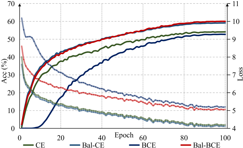
Figure 2: Training loss and Top-1% accuracy of ViT-S on iNaturalist 2018 dataset. Solid and dot lines represent the accuracy and training loss, respectively. All models adopt the same settings and random seed except for loss type.

Effectiveness of Proposed Bias. To learn balanced ViTs, we propose Bal-BCE with a simple yet effective logit bias (c.f. Eq. 10). To validate its effectiveness, we conduct the ablation study and compare it with the most popular re-balance loss, i.e., Bal-CE. As shown in Tab. 6, the new logit bias boosts vanilla BCE significantly with lower ECE on four ViT backbones, which is consistent with the behavior of Bal-CE. It is worth noticing that CE generally performs better than BCE in LTR scenarios, which is different from the conclusion in balanced datasets [55]. However, our Bal-BCE alleviates it remarkably and outperforms Bal-CE in most cases. In addition, Bal-BCE shows more satisfying numerical stability and faster convergence. See Bal-BCE in Fig. 2. for detailed illustrations.

For comprehensive comparisons, we re-implement recent rebalancing strategies in our BFT stage and show the results of ViT-B on CIFAR-LT in Tab. 7. Without loss of fairness, we conduct MGP on ImageNet-1K because the resolution (32$\times$32) of CIFAR is too small to mask for ViT-B-16. We do not reproduce the CL-based (conflict to MGP) and ensemble (memory limitation) methods. We also give up some ingenious rebalancing methods for loss NaN during training. As shown in Tab. 7, the proposed Bal-BCE achieves the best results, which firmly manifests its effectiveness. Notice that some methods are not consistent with their performance on ResNet, which means some exquisite designs may not generalize well on ViTs.

Hyper-Parameter Analysis. In Alg. 1 Line 11, we add a hyper-parameter $\tau$ to adjust our proposed bias (Eq. 10). We further present in-depth investigations on the influence of $\tau$. Similar to the aforementioned settings with plain augmentations, we conduct the ablation study on CIFAR-100-LT with MGP on ImageNet-1K and show the results in Fig.LABEL:fig:hyp-tau. The few-shot accuracy gets obvious amelioration when $\tau$ gets larger, which is consistent with our explanations in section 4.2. The best overall accuracy is obtained around $1$, which inspires us to set $\tau\equiv 1$ in LiVT for all experiments by default. Besides, the ECE gets smaller with increasing $\tau$, which means that the proposed bias guides ViTs to be the calibrated models with Fisher Consistency ensured [47].

Table 7: Ablation study of rebalancing strategies on ViT-B.

Method	CIFAR-10-LT		CIFAR-100-LT
$\gamma$	100	10	100	10
CE[13]	79.2	89.5	50.9	66.1
CB [13]	82.0	89.9	52.0	66.8
LDAM [4]	78.6	88.6	52.56	66.1
LADE [22]	68.8	81.7	56.7	68.2
IB [50]	75.4	79.2	50.8	51.6
Bal-CE [51]	84.4	90.7	56.8	68.1
Bal-BCE (ours)	86.3	91.3	58.2	69.2

6 Discussion

Why train from scratch? Previous ViTs papers are all based on pretrained weights from ImageNet-1K or ImageNet-22K and thus may lead to unfair comparisons with LTR methods, which are all trained from scratch. It is difficult to conclude that the intriguing performance mainly benefits from their proposals. Our approach provides a strong baseline to verify proposals’ effectiveness with ViTs. It’s also instructive to train plain ViTs for areas where data exhibits severe domain gaps. From the original intention of the LTR task, the core is to learn more large-scale imbalanced data effectively. Our work provides a feasible way to utilize more real-world LT (labels or attributes) data without expensive artificial balancing to achieve better representation learning.

How we extend MAE. We empirically prove that masked autoencoder learns generalized features even with imbalanced data, which is quite different from other self-supervised manners like CL [7] and SCL [30]. Extensive experiments on ImageNet-LT/BAL show that the instance number is more crucial than balanced annotation. We further propose the balanced binary cross-entropy loss to build our LiVT and achieve a new SOTA in LTR.

Limitations. One limitation is that LiVT can not be deployed in an end-to-end manner. An intuitive idea is two branches learning to optimize the decoder and classifier simultaneously, like BBN[81] or PaCo[12]. However, the heavily masked image prevents effective classification, while dynamic mask ratios exacerbate memory limitations.

7 Conclusion

In this paper, we propose to Learn imbalanced data with Vision Transformers (LiVT), which consists of Masked Generative Pretraining (MGP) and Balanced Fine Tuning (BFT). MGP is based on our empirical insight that it guides ViTs to learn more generalized features on long-tailed datasets compared to supervised or contrastive paradigms. BFT is based on the theoretical analysis of Binary Cross-Entropy (BCE) in the imbalanced scenario. We propose the balanced BCE to learn unbiased ViTs by compensating extra logit margins. Bal-BCE ameliorates BCE significantly and surpasses the powerful and widely adopted Balanced Cross-Entropy loss when cooperating with ViTs. Extensive experiments on large-scale datasets demonstrate that LiVT successfully trains ViTs without any additional data and achieves a new state-of-the-art for long-tail recognition.

Learning Imbalanced Data with Vision Transformers
Supplementary Material

Appendix A Missing Proofs and Derivations

A.1 Proof to Theorem 1

Theorem 1.  Logit Bias of Balanced CE. Let $\pi_{\mathbf{y}_{i}}=n_{\mathbf{y}_{i}}/N$ be the training label $\mathbf{y}_{i}$ distribution. If we implement the balanced cross-entropy loss via logit adjustment, the bias item of logit $\mathbf{z}_{\mathbf{y}_{i}}$ will be $\mathcal{B}^{\text{ce}}_{\mathbf{y}_{i}}=\log\pi_{\mathbf{y}_{i}}$, i.e.,

$$\mathcal{L}_{\text{Bal-CE}}=\log[1+\sum_{\mathbf{y}_{j}\neq\mathbf{y}_{i}}e^{(\mathbf{z}_{\mathbf{y}_{j}}+\log\pi_{\mathbf{y}_{j}})-(\mathbf{z}_{\mathbf{y}_{i}}+\log\pi_{\mathbf{y}_{i}})}].$$

Proof.

Following the notions in Section Preliminaries, we simplify a model $\mathcal{M}_{\theta}$ with parameters $\theta$, which attempts to learn the joint probability distribution of images and labels $\mathcal{P}(\mathcal{X},\mathcal{Y})$. Due to its agnostic, one may try to get the maximum posterior $\mathcal{P}(\mathcal{Y}|\mathcal{X})$ as an approximation solution from the Bayesian estimation view. To this end, if we Maximize A Posterior (MAP) to optimize $\theta$, we have:

$$\hat{\theta}=\arg\max_{\theta}\mathcal{P}(\mathcal{Y}|\mathcal{X})=\arg\max_{\theta}\frac{\mathcal{P}(\mathcal{X}|\mathcal{Y})\cdot\mathcal{P}(\mathcal{Y})}{\mathcal{P}(\mathcal{X})}=\arg\max_{\theta}\mathcal{P}(\mathcal{X}|\mathcal{Y})\cdot\mathcal{P}(\mathcal{Y}),$$

where $\mathcal{P}(\mathcal{X}|\mathcal{Y})$ is the likelihood function, $\mathcal{P}(\mathcal{Y})$ is the prior distribution of $\mathcal{Y}$, and $\mathcal{P}(\mathcal{X})$ is the evidence factor, which is $\theta$ irrelevant. Then, if we reasonably view $\mathcal{P}(\mathcal{Y})$ as the class distribution (typically class label frequency $\pi_{\mathbf{y}_{i}}$ as approximations), the MAP is equivalent to maximizing the likelihood function $\mathcal{P}(\mathcal{X}|\mathcal{Y};\theta)$. Considering both training $\mathcal{P}^{s}(\mathcal{X},\mathcal{Y})$ and test datasets $\mathcal{P}^{t}(\mathcal{X},\mathcal{Y})$, the MAP shall hold on to both of them, i.e.,

$$\left\{\begin{aligned} &\hat{\theta}=\arg\max_{\theta}\mathcal{P}^{s}(\mathcal{Y}|\mathcal{X})=\arg\max_{\theta}\mathcal{P}^{s}(\mathcal{X}|\mathcal{Y};\theta)\cdot\mathcal{P}^{s}(\mathcal{Y})\\ &\hat{\theta}=\arg\max_{\theta}\mathcal{P}^{t}(\mathcal{Y}|\mathcal{X})=\arg\max_{\theta}\mathcal{P}^{t}(\mathcal{X}|\mathcal{Y};\theta)\cdot\mathcal{P}^{t}(\mathcal{Y})\end{aligned}\right.$$

With model parameters $\theta$ learned on the training set $\mathcal{P}^{s}(\mathcal{X},\mathcal{Y})$, the likelihood function will be consistent. To obtain the maximization posterior on the test dataset (the best accuracy performance), we can derive that:

$$\mathcal{P}^{t}(\mathcal{Y}|\mathcal{X};\theta)\quad\propto\quad\mathcal{P}^{t}(\mathcal{X}|\mathcal{Y};\theta)\mathcal{P}^{t}(\mathcal{Y})\quad\propto\quad\frac{\mathcal{P}^{s}(\mathcal{Y}|\mathcal{X};\theta)}{\mathcal{P}^{s}(\mathcal{Y})}\cdot\mathcal{P}^{t}(\mathcal{Y})$$

Since MAP is equivalent to maximizing the likelihood function $\mathcal{P}(\mathcal{X}|\mathcal{Y};\theta)$, we further decouple the test MAP as regulation terms to achieve the Structural Risk Minimization:

$$\arg\max_{\theta}\mathcal{P}^{t}(\mathcal{Y}|\mathcal{X};\theta)\ =\ \arg\max_{\theta}\log\mathcal{P}^{t}(\mathcal{Y}|\mathcal{X};\theta)\ =\ \arg\max_{\theta}\log\mathcal{P}^{s}(\mathcal{X}|\mathcal{Y};\theta)-\log\mathcal{P}^{s}(\mathcal{Y})+\log\mathcal{P}^{t}(\mathcal{Y})$$

Notice that $\mathcal{P}^{s}(\mathcal{Y})$ and $\mathcal{P}^{t}(\mathcal{Y})$ are both $\theta$ irrelevant according to our previous hypothesis. Hence, we can compensate the regulation terms $-\log\mathcal{P}^{s}(\mathcal{Y})+\log\mathcal{P}^{t}(\mathcal{Y})$ during the training procession as $+\log\pi^{s}(\mathbf{y})-\log\pi^{t}(\mathbf{y})$. In addition, if we adopt the Softmax for probability normalization, we will have:

$$\mathcal{P}^{s}(\mathbf{x}_{i}|\mathbf{y}_{i};\theta)=\frac{e^{\mathbf{z}_{\mathbf{y}_{i}}}}{\sum_{\mathbf{y}_{j}\in\mathcal{C}}e^{\mathbf{z}_{\mathbf{y}_{j}}}}\quad\Longrightarrow\quad\log\mathcal{P}^{s}(\mathbf{x}_{i}|\mathbf{y}_{i};\theta)=\log\frac{e^{\mathbf{z}_{\mathbf{y}_{i}}}}{\sum_{\mathbf{y}_{j}\in\mathcal{C}}e^{\mathbf{z}_{\mathbf{y}_{j}}}}\quad\propto\quad\log e^{\mathbf{z}_{\mathbf{y}_{i}}}=\mathbf{z}_{\mathbf{y}_{i}}$$

Thus, the $\log\mathcal{P}^{s}(\mathcal{X}|\mathcal{Y};\theta)$ is equivalent to the output logits $\mathbf{z}:=\mathcal{M}(\mathbf{x}|\theta)$ and we immediately deduce that the training regulation shall be $\mathbf{z}_{\mathbf{y}}+\log\pi^{s}_{\mathbf{y}}-\log\pi^{t}_{\mathbf{y}}$. For the balanced test datasets, $-\log\pi^{t}_{\mathbf{y}}=\log C$ and can be ignored for all classes. Hence, we derive the final bias as:

$$\mathcal{B}^{\text{ce}}_{\mathbf{y}_{i}}=\log\pi^{s}_{\mathbf{y}_{i}}$$

∎

A.2 Proof to Theorem 2&3

Theorem 2&3.  Logit Bias of Balanced BCE with Test Prior. Let $\pi^{s}_{\mathbf{y}_{i}}$ and $\pi^{t}_{\mathbf{y}_{i}}$ be the label $\mathbf{y}_{i}$ training and test distribution. If we implement the balanced cross-entropy loss via logit adjustment, the bias item of logit $\mathbf{z}_{\mathbf{y}_{i}}$ will be:

$$\mathcal{B}^{\text{bce}}_{\mathbf{y}_{i}}=(\log\pi^{s}_{\mathbf{y}_{i}}-\log\pi^{t}_{\mathbf{y}_{i}})-(\log(1-\pi^{s}_{\mathbf{y}_{i}})-\log(1-\pi^{t}_{\mathbf{y}_{i}}))$$

Proof.

In this paper, we propose the balanced binary cross entropy loss in Thm. 2 and further extend it with the test prior (test label distribution) in Thm. 3. As we discussed, the bias in Thm. 2 is derived from re-balancing with training instance numbers like [51] do. Here, we give another proof from the Bayesian estimation view like Thm. 1. We mainly give the proof to the Thm. 3 and derive the Thm. 2 as a special case of Thm. 3. Following the notions in the proof to Thm. 1, BCE loss treats the long-tailed recognition task as $C$ independent binary classification problems. For every single problem, the derivation in Thm. 1 still holds if $\mathcal{Y}:=\{0,1\}$:

$$\arg\max_{\theta}\mathcal{P}^{t}(\mathcal{Y}|\mathcal{X};\theta)\ =\ \arg\max_{\theta}\log\mathcal{P}^{t}(\mathcal{Y}|\mathcal{X};\theta)\ =\ \arg\max_{\theta}\log\mathcal{P}^{s}(\mathcal{X}|\mathcal{Y};\theta)-\log\mathcal{P}^{s}(\mathcal{Y})+\log\mathcal{P}^{t}(\mathcal{Y})$$

If we adopt the Sigmoid for probability normalization, we will have:

$$\mathcal{P}^{s}(\mathbf{x}_{i}|\mathbf{y}_{i};\theta)=\frac{1}{1+e^{{-\mathbf{z}_{\mathbf{y}_{i}}}}}\quad\Longrightarrow\quad\frac{e^{{\mathbf{z}_{\mathbf{y}_{i}}}}}{e^{{\mathbf{z}_{\mathbf{y}_{i}}}}+e^{0}}$$

Similar to the Softmax, for the binary classification, we consider the ${e^{{\mathbf{z}_{\mathbf{y}_{i}}}}}/{(e^{{\mathbf{z}_{\mathbf{y}_{i}}}}+e^{0})}$ as the likelihood for $\mathcal{Y}=1$ and ${e^{0}}/{(e^{{\mathbf{z}_{\mathbf{y}_{i}}}}+e^{0})}$ for $\mathcal{Y}=0$. Then, we can derive that:

$$\log\mathcal{P}^{s}(\mathbf{x}_{i}|\mathbf{y}_{i};\theta)=\log\frac{e^{{\mathbf{z}_{\mathbf{y}_{i}}}}}{e^{{\mathbf{z}_{\mathbf{y}_{i}}}}+e^{0}}\quad\propto\quad\log e^{\mathbf{z}_{\mathbf{y}_{i}}}=\mathbf{z}_{\mathbf{y}_{i}}$$

Different from CE, which just punishes the positive term, BCE shall take the negative terms into consideration as well. If we take the statistical label frequency $\pi^{s}_{\mathbf{y}}$ and $\pi^{t}_{\mathbf{y}}$ as the prior, we can deduce that the bias should be:

$$\left\{\begin{aligned} &\log\pi^{s}_{\mathbf{y}}-\log\pi^{t}_{\mathbf{y}}\quad\quad\quad\quad\quad\quad\quad\text{{for positive item} $\mathbf{z}_{\mathbf{y}_{i}}$}\\ &\log(1-\pi^{s}_{\mathbf{y}})-\log(1-\pi^{t}_{\mathbf{y}})\quad\quad\ \text{{for negative item} $0$}\end{aligned}\right.$$

Hence, for a single binary classification, the unbiased Sigmoid operation is required to compensate for each term:

$$\sigma(\mathbf{z}_{\mathbf{y}_{i}})=\frac{e^{{\mathbf{z}_{\mathbf{y}_{i}}}}}{e^{{\mathbf{z}_{\mathbf{y}_{i}}}}+e^{0}}\Longrightarrow\frac{e^{{\mathbf{z}_{\mathbf{y}_{i}}}+\log\pi^{s}_{\mathbf{y}_{i}}-\log\pi^{t}_{\mathbf{y}_{i}}}}{e^{{\mathbf{z}_{\mathbf{y}_{i}}}+\log\pi^{s}_{\mathbf{y}_{i}}-\log\pi^{t}_{\mathbf{y}_{i}}}+e^{0+\log(1-\pi^{s}_{\mathbf{y}_{i}})-\log(1-\pi^{t}_{\mathbf{y}_{i}})}}$$

To match the Logit Adjustment requirement [47], we convert all bias to the logit $\mathbf{z}_{\mathbf{y}_{i}}$:

$$\sigma(\mathbf{z}_{\mathbf{y}_{i}})=\frac{e^{{\mathbf{z}_{\mathbf{y}_{i}}}}}{e^{{\mathbf{z}_{\mathbf{y}_{i}}}}+e^{0}} \Longrightarrow\frac{e^{{\mathbf{z}_{\mathbf{y}_{i}}}+\log\pi^{s}_{\mathbf{y}_{i}}-\log\pi^{t}_{\mathbf{y}_{i}}-(\log(1-\pi^{s}_{\mathbf{y}_{i}})-\log(1-\pi^{t}_{\mathbf{y}_{i}}))}}{e^{{\mathbf{z}_{\mathbf{y}_{i}}}+\log\pi^{s}_{\mathbf{y}_{i}}-\log\pi^{t}_{\mathbf{y}_{i}}-(\log(1-\pi^{s}_{\mathbf{y}_{i}})-\log(1-\pi^{t}_{\mathbf{y}_{i}}))}+e^{0}}$$

$$=\frac{1}{1+e^{-[{\mathbf{z}_{\mathbf{y}_{i}}}+(\log\pi^{s}_{\mathbf{y}_{i}}-\log\pi^{t}_{\mathbf{y}_{i}})-(\log(1-\pi^{s}_{\mathbf{y}_{i}})-\log(1-\pi^{t}_{\mathbf{y}_{i}}))]}}$$

Hence, we get the final bias with train and test label prior knowledge:

$$\mathcal{B}^{\text{bce}}_{\mathbf{y}_{i}}=(\log\pi^{s}_{\mathbf{y}_{i}}-\log\pi^{t}_{\mathbf{y}_{i}})-(\log(1-\pi^{s}_{\mathbf{y}_{i}})-\log(1-\pi^{t}_{\mathbf{y}_{i}}))$$

For the balanced test dataset, $\pi^{t}_{\mathbf{y}_{i}}=1/C$ and the $\mathcal{B}^{\text{bce}}_{\mathbf{y}_{i}}$ will be the form in Thm. 2 if we ignore constant terms.

$$\mathcal{B}^{\text{bce}}_{\mathbf{y}_{i}}=(\log\pi^{s}_{\mathbf{y}_{i}}-\log\frac{1}{C})-(\log(1-\pi^{s}_{\mathbf{y}_{i}})-\log(1-\frac{1}{C}))=\log\pi^{s}_{\mathbf{y}_{i}}-\log(1-\pi^{s}_{\mathbf{y}_{i}})+\log(C-1)$$

∎

A.3 Fisher Consistency with Test Prior

Menon et al. show how to verify whether a pair-wise loss ensures Fisher consistency for the balanced error (see the Theorem 1 in [47]). Here, we extend it to test the prior available situations.

$$\mathcal{L}(\mathbf{y}_{i},\mathcal{M}(\mathbf{x}))=\alpha_{\mathbf{y}_{i}}\cdot\log[1+\sum_{\mathbf{y}_{j}\neq\mathbf{y}_{i}}Exp(\Delta_{\mathbf{y}_{i}\mathbf{y}_{j}})\cdot Exp(\mathcal{M}_{\mathbf{y}_{j}}(\mathbf{x})-\mathcal{M}_{\mathbf{y}_{i}}(\mathbf{x}))]$$

Theorem 4. For any $\delta^{{s}},\delta^{{t}}\in\mathbb{R}_{+}^{{C}}$, the pairwise loss is Fisher consistent with weights and margins:

$$\alpha_{\mathbf{y}_{i}}=\frac{\delta_{\mathbf{y}_{i}}^{s}\cdot\pi_{\mathbf{y}_{i}}^{t}}{\delta_{\mathbf{y}_{i}}^{t}\cdot\pi_{\mathbf{y}_{i}}^{s}}\quad\Delta_{\mathbf{y}_{i}\mathbf{y}_{j}}=\log\left(\frac{\delta_{\mathbf{y}_{j}}^{s}\cdot\delta_{\mathbf{y}_{i}}^{t}}{\delta_{\mathbf{y}_{j}}^{t}\cdot\delta_{\mathbf{y}_{i}}^{s}}\right)$$

With $\delta_{\mathbf{y}_{i}}^{s}=\pi_{\mathbf{y}_{i}}^{s}$ and $\delta_{\mathbf{y}_{i}}^{t}=\pi_{\mathbf{y}_{i}}^{t}$, we deduce that Bal-BCE is Fisher consistent between train (s) and test (t) set.

Proof.

Let $\Delta_{{\mathbf{y}_{i}}{\mathbf{y}_{j}}}=\log\left(\frac{\delta_{\mathbf{y}_{j}}^{s}\cdot\delta_{\mathbf{y}_{i}}^{t}}{\delta_{\mathbf{y}_{j}}^{t}\cdot\delta_{\mathbf{y}_{i}}^{s}}\right)$ and $\alpha_{\mathbf{y}_{i}}=1$, we have:

$$\mathcal{L}(\mathbf{y}_{i},\mathcal{M}(\mathbf{x}))=-\log\frac{{e}^{\mathbf{z}_{\mathbf{y}_{i}}+\log\delta_{\mathbf{y}_{i}}^{s}-\log\delta_{\mathbf{y}_{i}}^{t}}}{\sum_{\mathbf{y}_{j}\in\mathcal{Y}}e^{\mathbf{z}_{\mathbf{y}_{j}}+\log\delta_{\mathbf{y}_{j}}^{s}-\log\delta_{\mathbf{y}_{j}}^{t}}}$$

If $\eta_{\mathbf{y}_{i}}(\mathbf{x})$ represents the posterior possibility $\mathcal{P}^{s}(\mathbf{y}_{i}|\mathbf{x})$, the Bayes-optimal score will satisfy:

$$\mathbf{z}^{*}_{\mathbf{y}_{i}}+\log\delta_{\mathbf{y}_{i}}^{s}-\log\delta_{\mathbf{y}_{i}}^{t}=\log\eta_{\mathbf{y}_{i}}(\mathbf{x})\quad\Longrightarrow\quad\mathbf{z}^{*}_{\mathbf{y}_{i}}=\log\left(\frac{\eta_{\mathbf{y}_{i}}(\mathbf{x})}{\delta_{\mathbf{y}_{i}}^{s}}\cdot\delta_{\mathbf{y}_{i}}^{t}\right)$$

Now consider adding weights $\alpha_{\mathbf{y}_{i}}$ to the loss term, the corresponding risk shall be:

$$\mathbb{E}_{\mathbf{x},\mathbf{y}}\left[\mathcal{L}_{\alpha_{\mathbf{y}_{i}}}\right]\quad=\quad\sum_{\mathbf{y}_{i}\in\mathcal{Y}}\pi_{\mathbf{y}_{i}}^{s}\cdot\mathbb{E}_{\mathbf{x}\mid\mathbf{y}=\mathbf{y}_{i}}\left[\mathcal{L}_{\alpha_{\mathbf{y}_{i}}}\right]\quad=\quad\sum_{\mathbf{y}_{i}\in\mathcal{Y}}\pi_{\mathbf{y}_{i}}^{s}\cdot\alpha_{\mathbf{y}i}\cdot\mathbb{E}_{\mathbf{x}\mid\mathbf{y}=\mathbf{y}_{i}}[\mathcal{L}]\quad\propto\quad\sum_{\mathbf{y}_{i}\in\mathcal{Y}}\bar{\pi}_{\mathbf{y}_{i}}^{s}\cdot\mathbb{E}_{\mathbf{x}\mid\mathbf{y}=\mathbf{y}_{i}}[\mathcal{L}]$$

where $\bar{\pi}_{\mathbf{y}_{i}}^{s}\propto\pi_{\mathbf{y}_{i}}^{s}\cdot\alpha_{\mathbf{y}_{i}}$. Hence training with the weighted loss amounts to training with the original loss on the new label distribution $\bar{\pi}$. The posterior probability $\bar{\eta}_{\mathbf{y}_{i}}(\mathbf{x})$ on the altered label distribution is:

$$\bar{\eta}_{\mathbf{y}_{i}}(\mathbf{x})=\overline{\mathcal{P}}\left(\mathbf{y}_{i}|\mathbf{x}\right)\quad\propto\quad\mathcal{P}\left(\mathbf{x}|\mathbf{y}_{i}\right)\cdot\bar{\pi}_{\mathbf{y}_{i}}^{s}\quad\propto\quad\eta_{\mathbf{y}_{i}}(\mathbf{x})\cdot\frac{\bar{\pi}_{\mathbf{y}_{i}}^{\mathrm{s}}}{\pi_{\mathbf{y}_{i}}^{s}}\quad\propto\quad\eta_{\mathbf{y}_{i}}(\mathbf{x})\cdot\alpha_{\mathbf{y}_{i}}$$

When we set $\alpha_{\mathbf{y}_{i}}=\frac{\delta_{\mathbf{y}_{i}}^{s}\cdot\pi_{\mathbf{y}_{i}}^{t}}{\delta_{\mathbf{y}_{i}}^{t}\cdot\pi_{\mathbf{y}_{i}}^{s}}$, the Bayes-optimal score will satisfy:

$$\arg\max_{\mathbf{y}_{i}\in\mathcal{Y}}\mathbf{z}_{\mathbf{y}_{i}}^{*} =\quad\arg\max_{\mathbf{y}_{i}\in\mathcal{Y}}\log\left(\frac{\bar{\eta}_{\mathbf{\mathbf{y}_{i}}}(\mathbf{x})}{\delta_{\mathbf{y}_{i}}^{s}}\cdot\delta_{\mathbf{y}_{i}}^{t}\right)\quad$$

$$=\quad\arg\max_{\mathbf{y}_{i}\in\mathcal{Y}}\log\left(\frac{\eta_{\mathbf{y}_{i}}(\mathbf{x})\cdot\alpha_{\mathbf{y}_{i}}}{\delta_{\mathbf{y}_{\mathbf{i}}}^{s}}\cdot\delta_{\mathbf{y}_{i}}^{t}\right)\quad$$

$$=\quad\arg\max_{\mathbf{y}_{i}\in\mathcal{Y}}\log\left(\frac{\eta_{\mathbf{y}_{i}}(\mathbf{x})}{\pi_{\mathbf{y}_{i}}^{s}}\cdot\pi_{\mathbf{y}_{i}}^{t}\right)$$

∎

Appendix B Analysis to Proposed Bias

Figure 4: $\mathcal{B}^{\text{ce}}_{\mathbf{y}_{i}}$ and $\mathcal{B}^{\text{bce}}_{\mathbf{y}_{i}}$ w.r.t. $\pi_{\mathbf{y}_{i}}$ ($C$=1,000).

For Bal-CE, Ren et al. [51] propose the balanced softmax as a strong baseline for long-tailed recognition while Menon et al [47] deploy it by adding extra logit margins. The following works [22, 70] further extend it with test prior knowledge, which can be written as:

$$\mathcal{B}^{\text{ce}}_{\mathbf{y}_{i}}=\log\pi^{s}_{\mathbf{y}_{i}}+\log C$$

To improve the performance of balanced binary cross-entropy loss in long-tailed recognition, we propose an unbiased version of Sigmoid to eliminate the inherent bias to the head class. Inspired by Logit Adjustment [47], we implement it as a bias $\mathcal{B}^{\text{bce}}_{\mathbf{y}_{i}}$ to the model logits and extend to test prior as well, which can be written as:

$$\mathcal{B}^{\text{bce}}_{\mathbf{y}_{i}}=\log\pi^{s}_{\mathbf{y}_{i}}-\log(1-\pi^{s}_{\mathbf{y}_{i}})+\log(C-1)$$

Fig. 4 shows the difference between $\mathcal{B}^{\text{ce}}_{\mathbf{y}_{i}}$ and $\mathcal{B}^{\text{bce}}_{\mathbf{y}_{i}}$. Notice that $\mathcal{B}^{\text{bce}}_{\mathbf{y}_{i}}$ is closed to $\mathcal{B}^{\text{ce}}_{\mathbf{y}_{i}}$ when $\pi_{\mathbf{y}_{i}}$ is small, which indicates that both $\mathcal{B}^{\text{ce}}_{\mathbf{y}_{i}}$ and $\mathcal{B}^{\text{bce}}_{\mathbf{y}_{i}}$ help the models to pay more attention to learn the tail. However, $\mathcal{B}^{\text{bce}}_{\mathbf{y}_{i}}$ gives larger biases to the head and makes the inter-class distance of the head smaller. Such a modification allows Bal-BCE to show more tolerance to the head compared to Bal-CE. To be more specific, CE utilizes Softmax to emphasize mutual exclusion, where large head bias will damage corresponding performance severely. In contrast, BCE calculates independent class-wise probability with Sigmoid function, where the original task is considered as a series of binary classification tasks. Hence, the head bias will not influence the tail. In addition, larger biases will not hurt the head as CE does because it hedges the over-suppression for negative labels. CE can not benefit from it because of its mutual exclusion.

$$\left\{\begin{aligned} &\frac{\partial\mathcal{L}_{\text{Bal-CE}}\left(\mathbf{z}_{\mathbf{y}_{j}},\mathbbm{1}({\mathbf{y}_{j}})\right)}{\partial\left(\mathbf{z}_{\mathbf{y}_{j}}\right)}=\frac{e^{\mathbf{z}_{\mathbf{y}_{j}}+\mathcal{B}^{\text{ce}}_{\mathbf{y}_{j}}}}{\sum_{\mathbf{y}_{i}\in\mathcal{C}}e^{\mathbf{z}_{\mathbf{y}_{i}}+\mathcal{B}^{\text{ce}}_{\mathbf{y}_{i}}}},\quad\frac{\partial\mathcal{L}_{\text{Bal-BCE}}\left(\mathbf{z}_{\mathbf{y}_{j}},\mathbbm{1}({\mathbf{y}_{j}})\right)}{\partial\left(\mathbf{z}_{\mathbf{y}_{j}}\right)}=\frac{e^{\mathbf{z}_{\mathbf{y}_{j}}+\mathcal{B}^{\text{bce}}_{\mathbf{y}_{j}}}}{1+e^{\mathbf{z}_{\mathbf{y}_{j}}+\mathcal{B}^{\text{bce}}_{\mathbf{y}_{j}}}},\quad\ \ \ \mathbbm{1}({\mathbf{y}_{j}})=0\\ &\frac{\partial\mathcal{L}_{\text{Bal-CE}}\left(\mathbf{z}_{\mathbf{y}_{j}},\mathbbm{1}({\mathbf{y}_{j}})\right)}{\partial\left(\mathbf{z}_{\mathbf{y}_{j}}\right)}=\frac{e^{\mathbf{z}_{\mathbf{y}_{j}}+\mathcal{B}^{\text{ce}}_{\mathbf{y}_{j}}}}{\sum_{\mathbf{y}_{i}\in\mathcal{C}}e^{\mathbf{z}_{\mathbf{y}_{i}}+\mathcal{B}^{\text{ce}}_{\mathbf{y}_{i}}}},\quad\frac{\partial\mathcal{L}_{\text{Bal-BCE}}\left(\mathbf{z}_{\mathbf{y}_{j}},\mathbbm{1}({\mathbf{y}_{j}})\right)}{\partial\left(\mathbf{z}_{\mathbf{y}_{j}}\right)}=-\frac{1}{1+e^{\mathbf{z}_{\mathbf{y}_{j}}+\mathcal{B}^{\text{bce}}_{\mathbf{y}_{j}}}},\quad\mathbbm{1}({\mathbf{y}_{j}})=1\end{aligned}\right.$$

From the optimization view, as the above equation shows, we can also observe that $\mathcal{B}^{\text{bce}}_{\mathbf{y}_{i}}$ will not affect class $\mathbf{y}_{j}$’s gradients. However, for Bal-CE, the optimization step would be rather small once the logit for the positive class is much higher than those of the negative ones. With the dominance of head labels, larger head biases will make the networks fall into even worse situations. In contrast, for the Bal-BCE, the above larger head biases will act as a regularization to overcome the over-suppression while avoiding damage to the head classes themselves.

In addition, $\mathcal{B}^{\text{bce}}_{\mathbf{y}_{i}}$ will be more important when the datasets become more skewed. As Fig. 5 shows, the difference will be larger when the imbalance factor $\gamma$ increases. It means the performance will get worse if we adopt $\mathcal{B}^{\text{ce}}_{\mathbf{y}_{i}}$ for BCE loss. Notice that the gap between $\mathcal{B}^{\text{ce}}_{\mathbf{y}_{i}}$ and $\mathcal{B}^{\text{bce}}_{\mathbf{y}_{i}}$ has consistent diminution when the class number $C$ is getting bigger. However, $\mathcal{B}^{\text{bce}}_{\mathbf{y}_{i}}$ still bring obvious performance gain in this circumstance.

\begin{overpic}[scale={0.35},grid=False,tics=5]{Figs/apdx/vis_cifar.pdf} \put(10.5,0.0){\scriptsize{$\gamma=10$}} \put(36.0,0.0){\scriptsize{$\gamma=50$}} \put(60.0,0.0){\scriptsize{$\gamma=100$}} \put(85.0,0.0){\scriptsize{$\gamma=200$}} \end{overpic}

Figure 5: Visualization of the bias in CIFAR10-LT dataset. A larger $\gamma$ indicates a severer imbalance situation. $\Delta$ is the difference between the two biases, which is shown in right y-axis. With $\gamma$ increases, the $\Delta$ becomes more important to the final bias.

Appendix C Datasets

We conduct experiments on CIFAR-LT [32], ImageNet-LT [52], iNat18 [57], and Places-LT [82]. With different imbalanced factors $\gamma$, we build the long-tailed version of CIFAR by discarding training instances following the rule given in [13] and keeping the original validation set for all datasets. To investigate the MGP performance on LT data, we build a balanced ImageNet-1K subset called ImageNet-BAL. It contains the same training instance number as ImageNet-LT while keeping class labels balanced. Notice that both LT and BAL adopt the same validation set. We demonstrate MGP is robust enough for long-tailed data via quantitative and qualitative experiments on the BAL and LT. iNat18 is the largest benchmark of the long tail community. Our LiVT ameliorates vanilla ViTs most significantly because of the data scale and fine-grained problems. Places-LT is created from large-scale dataset Places [82] by [44]. The train set contains just 62K images with a high imbalance factor, which makes it challenging for data-hungry Transformers.

Table 8: Detailed information of datasets motioned in the main paper.

Dataset	CIFAR-10-LT		CIFAR-100-LT		ImageNet-LT	ImageNet-BAL	iNat18	PlaceLT
	Imbalance Factor ($\gamma$)
	100	10	100	10
Training Images	12,406	20,431	10,847	19,573	115,846	160,000	437,513	62,500
Classes Number	10	10	100	100	1,000	1,000	8,142	365
Max Images	5,000	5,000	500	500	1,280	160	1,000	4,980
Min Images	50	500	5	50	5	160	2	5
Imbalance Factor	100	10	100	10	256	1	500	996

Appendix D Implementation Details

D.1 Augmentations in Algorithm.1

In Alg. 1, LiVT adopts different augmentations in two stages, i.e., $\mathcal{A}_{pt}$ & $\mathcal{A}_{ft}$. The reason is from our observations that the strong data augmentations in MGP will not contribute to higher performance while bringing extra calculation burden. Some augmentations like Color Jitter may lead to wired reconstruction results w.r.t. the augmented images. For the BFT stage, we adopt more general data augmentations for stable training procession. The AutoAug improves performance on ImageNet-LT/BAL remarkably and slightly in iNat18 / Places-LT, which is consistent with the observation in [12]. Mixup and Cutmix make the training more smooth, and RandomErease regulates the model with better performance.

Table 9: The detailed augmentations adopted in Alg. 1.

Augmentation	Masked Generative Pretraining ($\mathcal{A}_{pt}$)	Balanced Fine Tuning ($\mathcal{A}_{ft}$)
RandomResizedCrop	✓	✓
RandomHorizontalFlip	✓	✓
AutoAug	$\times$	(9,0.5)
Mixup	$\times$	0.8
Cutmix	$\times$	1.0
RandomErease	$\times$	0.25
Normalize	✓	✓

D.2 Configure Settings for Table 1

In Tab. 1, we implement different ViT training recipes on long-tailed and balanced ImageNet-1K subsets. Specially, we reproduce vanilla ViTs according to Tab.11 in [18], DeiT III according to Tab.1 in [55], and MAE according to Tab.9 in [18]. All recipes train ViTs with more epochs (800) compared to ResNets (typically 90 or 180). However, the performance is far from catching up with ResNet baselines and severely deteriorate when it becomes imbalanced because the dataset is relatively small for data-hungry ViTs compared to ImageNet-1K or ImageNet22K and the long-tailed labels bias the ViTs heavily.

D.3 Configure Settings for the Main Comparisons

We conduct experiments on ImageNet-LT, iNat18, and Places-LT. For fair comparisons, we train all models from scratch following previous LTR work. To balance the performance and computation complexity trade-off, we adopt a small image size for the large-scale dataset and adopt 800 epochs for MGP. Thanks to the masked tokens, MGP trains ViTs much faster than vanilla ViT and DeiT. We transfer the hyper-parameters of ImageNet-LT to other benchmarks and just finetune the $\tau$ of Bal-BCE loss slightly. Notice that Places-LT is a small dataset and we just finetune 30 epochs to avoid over-fitting.

Table 10: The LiVT configurations on three main benchmarks. We mainly transfer the hyper-parameters of ImageNet-LT to other benchmarks without wide changes. Tuning hyper-parameters will bring further improvement.

Configuration	ImageNet-LT	iNaturalist 2018	Places-LT
Masked Generative Pretraining.
Epoch	800	800	800
Warmup Epoch	40	40	40
Effective Batch Size	4096	4096	4096
Optimizer	AdamW(0.9,0.95)	AdamW(0.9,0.95)	AdamW(0.9,0.95)
Learning Rate	1.5e-4	1.5e-4	1.5e-4
LR schedule	cosine(min=0)	cosine(min=0)	cosine(min=0)
Weight Decay	5e-2	5e-2	5e-2
Mask Ratio	0.75	0.75	0.75
Input Size	224	128	224
Balanced Fine Tuning.
Epoch	100	100	30
Warmup Epoch	10	10	5
Effective Batch Size	1024	1024	1024
Optimizer	AdamW(0.9,0.99)	AdamW(0.9,0.99)	AdamW(0.9,0.99)
Learning Rate	1e-3	1e-3	1e-3
LR schedule	cosine(min=1e-6)	cosine(min=1e-6)	cosine(min=1e-6)
Weight Decay	5e-2	5e-2	5e-2
Layer Decay	0.75	0.75	0.75
Input Size	224	224	224
Drop Path	0.1	0.2	0.1
$\tau$ of Bal-BCE	1	1	1.05

Appendix E Additional Experiments

E.1 DeiT with Bal-BCE

In the DeiT III [55], Touvron et al. propose to train ViTs with binary cross entropy loss. With our proposed bias $\mathcal{B}^{\text{bce}}$, we can further boost its recipe when collaborating with long-tailed distributed data. As Tab. 11 shows, Bal-BCE rebalances the performance of ViT-Small over three groups and improves the overall accuracy significantly. It is worth noticing that the few-shot gets ameliorated remarkably, while the many-shot is sacrificed to some extent. Compared to the results in Tab.6, we get a meticulous observation that Bal-BCE improves all groups’ performance when adopting MGP as the pretrain manner, and even the many-shot (head) classes get compelling growth, especially on the small models. The aforementioned phenomenon may indicate that the MGP learns more generalized and unbiased features compared to supervised manners, which helps $\mathcal{B}^{\text{bce}}$ to calibrate more misclassification cases instead of the over-confident but right cases.

Table 11: Ablation study of proposed bias on DeiT III. Experiments are conducted with ViT-Small on ImageNet-LT for 400 epochs.

Loss Type	Many	$\Delta$	Med.	$\Delta$	Few	$\Delta$	Acc	$\Delta$
BCE w/o $\mathcal{B}^{\text{bce}}$	64.2	-	32.2	-	9.0	-	41.4	-
BCE w/ $\mathcal{B}^{\text{bce}}$	60.3	-4.0	40.8	+8.7	23.8	+14.7	46.0	+4.6

E.2 Performance with higher resolution

With the FixRes effect [56], LiVT can reach further performance gains with minor computational overhead, which only increases the resolution in the 2nd stage with a few epochs. As a comparison, ResNet-based methods require extra effort to modify the network with heavy computational overhead. Hence, we only provide LiVT^∗ in Tab. 2-4. Note that LiVT with 224 resolution already achieves SOTA performance (except tiny Places-LT). We additionally show ViT-based methods with 384 resolution in Tab. 12. ViT-based methods typically show lower performance than ResNet-based ones due to ViTs’ data hungry in the tiny dataset (Tab. 4). Noteworthy, our Bal-BCE loss remarkably improves performance (Acc +10.5% & Few +18.8% compared to MAE). While tuning hyper-parameters (e.g., $\tau$ in Alg. 1 or parameters in Tab. 9&10) can further boost the performance (Fig. LABEL:fig:hyp-tau), we keep consistent settings with Tab. 2&3 to report the LiVT performance in Tab. 4.

Table 12: Top-1 Accuracy of ViT-B-16 pretrained on iNat18 dataset. We fine-tune models for 100 epochs with 384 resolution.

Resolution	ViT	DeiT	MAE	LiVT
224 $\times$ 224	54.6	61.0	69.4	76.1
384 $\times$ 384	56.3 +1.7	63.7 +2.7	72.9 +3.5	81.0 +4.9

E.3 Negative-Tolerant Regularization

Recently, there are some other works to improve the performance of BCE loss. For instance, Wu et al. [66] propose to leave more Negative Tolerant Regularization (NTR) in the BCE loss. In long-tailed recognition, the tail class samples are usually learned as negative pairs resulting from the head class dominance. Here, for clear and concise expression, we call the logit $z_{\mathbf{y}_{i}}$ positive logit and $z_{\mathbf{y}_{j}},(j\neq i)$ negative logits for the label $\mathbf{y}_{i}$. For Softmax operation, the gradient of the negative logits will be relatively small due to its mutual exclusion when the positive logit is large. However, Sigmoid acts differently from Softmax. The Sigmoid always maintains relatively large gradients for negative logits despite the positive logit value. This property of BCE leads to the output tail class logits being smaller, which incurs that the model only overfits a few tail-positive samples in the training set.

To overcome this problem, Wu et al. propose the NT-BCE loss to alleviate the dominance of negative labels. With a hyper-parameter $\lambda$ to control the strength of negative tolerance regularization, the NT-BCE can be written as:

$$\mathcal{L}_{\text{NT-BCE}}=-\sum_{\mathbf{y}_{i}\in\mathcal{C}} [\mathbbm{1}(\mathbf{y}_{i})\cdot\log\frac{1}{1+e^{-\mathbf{z}_{\mathbf{y}_{i}}}}+\frac{1}{\lambda}(1-\mathbbm{1}(\mathbf{y}_{i}))\cdot\log(1-\frac{1}{1+e^{-\lambda\mathbf{z}_{\mathbf{y}_{i}}}})]$$

To collaborate with it, we add our proposed bias $\mathcal{B}^{\text{bce}}_{\mathbf{y}_{i}}=\log\pi_{\mathbf{y}_{i}}-\log(1-\pi_{\mathbf{y}_{i}}))$ to the above loss and derive that:

$$\mathcal{L}^{*}_{\text{NT-BCE}}=-\sum_{\mathbf{y}_{i}\in\mathcal{C}} [\mathbbm{1}(\mathbf{y}_{i})\cdot\log\frac{1}{1+e^{-(\mathbf{z}_{\mathbf{y}_{i}}+\mathcal{B}^{\text{bce}}_{\mathbf{y}_{i}})}}+\frac{1}{\lambda}(1-\mathbbm{1}(\mathbf{y}_{i}))\cdot\log(1-\frac{1}{1+e^{-\lambda(\mathbf{z}_{\mathbf{y}_{i}}+\mathcal{B}^{\text{bce}}_{\mathbf{y}_{i}})}})]$$

For more in-depth observations, we train ViT-B on CIFAT-100-LT with both $\mathcal{L}_{\text{NT-BCE}}$ and $\mathcal{L}^{*}_{\text{NT-BCE}}$ and show the experiment results in Fig. LABEL:fig:ntr. The NTR ameliorates the vanilla BCE loss with large $\lambda$ by benefiting medium and tail classes. However, the performance of $\mathcal{L}_{\text{NT-BCE}}$ is hard to catch up with $\mathcal{L}^{*}_{\text{NT-BCE}}$. What’s worse, the NTR consistently deteriorates the performance of $\mathcal{L}^{*}_{\text{NT-BCE}}$ when $\lambda$ gets larger. The best is achieved at $\lambda=1$, which indicates that NTR can not work well with our bias.

To explain it, we revisit the purpose of NTR, which aims to reduce the gradient of tail negative logits. While optimizing the tail class as negative logits, if the logit is small, the corresponding gradient will also be small to keep the logit from over-minimization. However, it is contradictory to our proposed bias. Typically, the margin-based loss makes the network pay attention to certain categories by increasing the corresponding difficulty with larger margins. As the margins for all classes, our bias $\mathcal{B}^{\text{bce}}$ makes the tail (head) class harder (easier) to learn, where the initial head logits are larger than tail ones, as shown in Fig.5. With NTR, tail classes will converge more slowly because larger $\lambda$ tends to slow down the optimization of tail logits, which finally results in unsatisfying tail performance. Although We et al., add a similar bias in [66], they ignore its effect because of the little difference between the training and test label distribution of their datasets. More explorations are still required to make NTR and $\mathcal{B}^{\text{bce}}$ complement each other in long-tailed recognition.

Appendix F More Discussions

F.1 About the two-stage pipeline.

Although one stage is a promising direction, the two-stage frameworks (e.g., c-RT [29], MiSLAS [80], and our LiVT) typically achieve much better performance. For ViTs in LTR tasks, the difficulty is to learn the inductive bias and label statistical bias simultaneously. We manage the challenge by decoupling the two biases and learning the inductive bias in the MGP stage and the statistical bias in the BFT stage separately.

F.2 Test prior to model performance.

The Bal-CE implementation in previous work [51] contains the test prior (i.e., $\pi_{i}^{t}=1/C$) by default. With balanced test data, it is equal to eliminate the test prior bias item $-\log\pi_{i}^{t}=\log C$ with Softmax operation (Eq. 2). However, for Bal-BCE, the test prior term cannot be reduced in Sigmoid operation. As we discussed in Thm. 3, although ignoring this term does not influence the optimization direction, it will reduce the loss value, especially when $C$ is large (c.f. derivation in Supp. A.2). Therefore, the test prior is essential to ensure stability during training in Bal-BCE (e.g., models trained in the iNat18 dataset cannot converge without this item).

F.3 About the baseline performance.

One may consider overfitting as a possible reason for the poor performance of the ViT baseline. Hence, we visualize the training log in Fig. 7. Either in the tiny Places-LT or the large-scale iNat18 (similar scale to ImageNet-1K), ViTs exhibit biased performance (Tab. 2-4). The unsatisfactory performance of ViT-based baselines (direct supervision) mainly accounts for the long-tailed problems rather than the overfitting issues (Tab. 1). Even under the same setting with these baselines, Bal-BCE improves MAE (Tab. 2-4) and DeiT (Supp. E.1) consistently in few and overall performance.

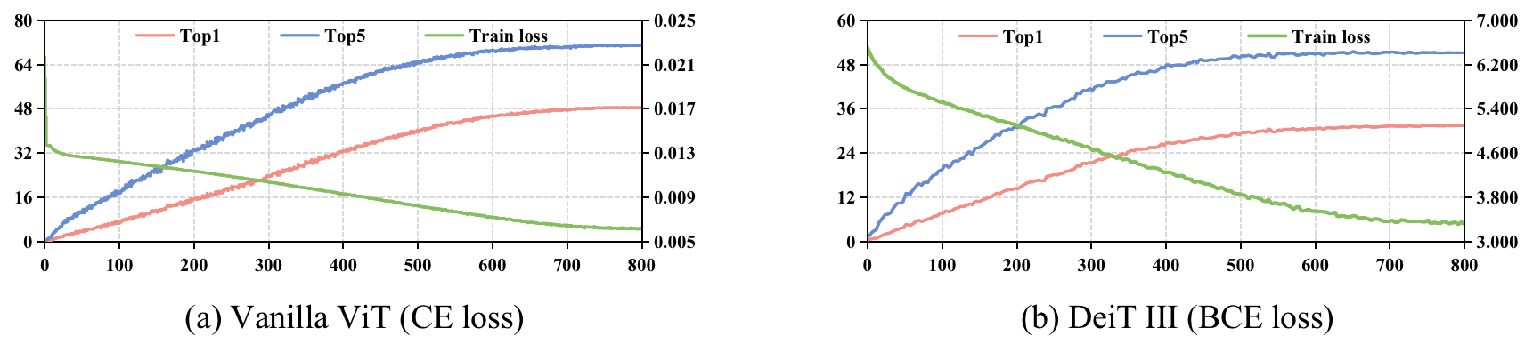
Figure 7: The training log of ViT-B on ImageNet-LT. Left y-axis: validation accuracy. Right y-axis: training loss value. The validation accuracy is consistent with training loss, which means that overfitting does not occur during the training process.

Appendix G Visualization of MGP Reconstruction

References

- [1] Shaden Alshammari, Yu-Xiong Wang, Deva Ramanan, and Shu Kong. Long-tailed recognition via weight balancing. In CVPR, pages 6897–6907, 2022.
- [2] Hangbo Bao, Li Dong, Songhao Piao, and Furu Wei. BEit: BERT pre-training of image transformers. In ICLR, 2022.
- [3] Jiarui Cai, Yizhou Wang, Jenq-Neng Hwang, et al. Ace: Ally complementary experts for solving long-tailed recognition in one-shot. In ICCV, pages 112–121, 2021.
- [4] Kaidi Cao, Colin Wei, Adrien Gaidon, Nikos Arechiga, and Tengyu Ma. Learning imbalanced datasets with label-distribution-aware margin loss. NeurIPS, 32, 2019.
- [5] Nicolas Carion, Francisco Massa, Gabriel Synnaeve, Nicolas Usunier, Alexander Kirillov, and Sergey Zagoruyko. End-to-end object detection with transformers. In ECCV, pages 213–229. Springer, 2020.
- [6] Huiwen Chang, Han Zhang, Lu Jiang, Ce Liu, and William T. Freeman. Maskgit: Masked generative image transformer. In CVPR, June 2022.
- [7] Ting Chen, Simon Kornblith, Mohammad Norouzi, and Geoffrey Hinton. A simple framework for contrastive learning of visual representations. In ICML, pages 1597–1607. PMLR, 2020.
- [8] Xinlei Chen, Saining Xie, and Kaiming He. An empirical study of training self-supervised vision transformers. In ICCV, pages 9640–9649, 2021.
- [9] Hsin-Ping Chou, Shih-Chieh Chang, Jia-Yu Pan, Wei Wei, and Da-Cheng Juan. Remix: rebalanced mixup. In ECCV, pages 95–110. Springer, 2020.
- [10] Peng Chu, Xiao Bian, Shaopeng Liu, and Haibin Ling. Feature space augmentation for long-tailed data. In ECCV, pages 694–710. Springer, 2020.
- [11] Ekin D Cubuk, Barret Zoph, Jonathon Shlens, and Quoc V Le. Randaugment: Practical automated data augmentation with a reduced search space. In CVPR workshops, pages 702–703, 2020.
- [12] Jiequan Cui, Zhisheng Zhong, Shu Liu, Bei Yu, and Jiaya Jia. Parametric contrastive learning. In ICCV, pages 715–724, 2021.
- [13] Yin Cui, Menglin Jia, Tsung-Yi Lin, Yang Song, and Serge Belongie. Class-balanced loss based on effective number of samples. In CVPR, pages 9268–9277, 2019.
- [14] Jacob Devlin, Ming-Wei Chang, Kenton Lee, and Kristina Toutanova. BERT: pre-training of deep bidirectional transformers for language understanding. In NAACL, pages 4171–4186. Association for Computational Linguistics, 2019.
- [15] Alexey Dosovitskiy, Lucas Beyer, Alexander Kolesnikov, Dirk Weissenborn, Xiaohua Zhai, Thomas Unterthiner, Mostafa Dehghani, Matthias Minderer, Georg Heigold, Sylvain Gelly, Jakob Uszkoreit, and Neil Houlsby. An image is worth 16x16 words: Transformers for image recognition at scale. In ICLR, 2021.
- [16] Christoph Feichtenhofer, Haoqi Fan, Yanghao Li, and Kaiming He. Masked autoencoders as spatiotemporal learners. arXiv preprint arXiv:2205.09113, 2022.
- [17] Chuan Guo, Geoff Pleiss, Yu Sun, and Kilian Q Weinberger. On calibration of modern neural networks. In ICML, pages 1321–1330. PMLR, 2017.
- [18] Kaiming He, Xinlei Chen, Saining Xie, Yanghao Li, Piotr Dollár, and Ross B. Girshick. Masked autoencoders are scalable vision learners. In CVPR, pages 15979–15988. IEEE, 2022.
- [19] Kaiming He, Haoqi Fan, Yuxin Wu, Saining Xie, and Ross Girshick. Momentum contrast for unsupervised visual representation learning. In CVPR, pages 9729–9738, 2020.
- [20] Kaiming He, Xiangyu Zhang, Shaoqing Ren, and Jian Sun. Deep residual learning for image recognition. In CVPR, pages 770–778, 2016.
- [21] Yin-Yin He, Jianxin Wu, Xiu-Shen Wei, et al. Distilling virtual examples for long-tailed recognition. In ICCV, pages 235–244, 2021.
- [22] Youngkyu Hong, Seungju Han, Kwanghee Choi, Seokjun Seo, Beomsu Kim, and Buru Chang. Disentangling label distribution for long-tailed visual recognition. In CVPR, pages 6626–6636, 2021.
- [23] Yan Hong, Jianfu Zhang, Zhongyi Sun, and Ke Yan. Safa: Sample-adaptive feature augmentation for long-tailed image classification. In ECCV, 2022.
- [24] Zhi Hou, Baosheng Yu, Dacheng Tao, et al. Batchformer: Learning to explore sample relationships for robust representation learning. In CVPR, 2022.
- [25] Ahmet Iscen, Andre Araujo, Boqing Gong, and Cordelia Schmid. Class-balanced distillation for long-tailed visual recognition. In BMVC, page 165. BMVA Press, 2021.
- [26] Muhammad Abdullah Jamal, Matthew Brown, Ming-Hsuan Yang, Liqiang Wang, and Boqing Gong. Rethinking class-balanced methods for long-tailed visual recognition from a domain adaptation perspective. In CVPR, pages 7610–7619, 2020.
- [27] Bingyi Kang, Yu Li, Sa Xie, Zehuan Yuan, and Jiashi Feng. Exploring balanced feature spaces for representation learning. In ICLR, 2020.
- [28] Bingyi Kang, Yu Li, Sa Xie, Zehuan Yuan, and Jiashi Feng. Exploring balanced feature spaces for representation learning. In ICLR, 2021.
- [29] Bingyi Kang, Saining Xie, Marcus Rohrbach, Zhicheng Yan, Albert Gordo, Jiashi Feng, and Yannis Kalantidis. Decoupling representation and classifier for long-tailed recognition. In ICLR, 2020.
- [30] Prannay Khosla, Piotr Teterwak, Chen Wang, Aaron Sarna, Yonglong Tian, Phillip Isola, Aaron Maschinot, Ce Liu, and Dilip Krishnan. Supervised contrastive learning. NeurIPS, 33:18661–18673, 2020.
- [31] Jaehyung Kim, Jongheon Jeong, Jinwoo Shin, et al. M2m: Imbalanced classification via major-to-minor translation. In CVPR, pages 13896–13905, 2020.
- [32] A. Krizhevsky and G. Hinton. Learning multiple layers of features from tiny images. Master’s thesis, Department of Computer Science, University of Toronto, 2009.
- [33] Bolian Li, Zongbo Han, Haining Li, Huazhu Fu, and Changqing Zhang. Trustworthy long-tailed classification. In CVPR, pages 6970–6979, 2022.
- [34] Jun Li, Zichang Tan, Jun Wan, Zhen Lei, and Guodong Guo. Nested collaborative learning for long-tailed visual recognition. In CVPR, pages 6949–6958, 2022.
- [35] Mengke Li, Yiu-ming Cheung, Yang Lu, et al. Long-tailed visual recognition via gaussian clouded logit adjustment. In CVPR, pages 6929–6938, 2022.
- [36] Tianhong Li, Peng Cao, Yuan Yuan, Lijie Fan, Yuzhe Yang, Rogerio S Feris, Piotr Indyk, and Dina Katabi. Targeted supervised contrastive learning for long-tailed recognition. In CVPR, pages 6918–6928, 2022.
- [37] Tianhao Li, Limin Wang, and Gangshan Wu. Self supervision to distillation for long-tailed visual recognition. In ICCV, pages 630–639, 2021.
- [38] Tsung-Yi Lin, Priya Goyal, Ross Girshick, Kaiming He, and Piotr Dollár. Focal loss for dense object detection. In ICCV, pages 2980–2988, 2017.
- [39] Tsung-Yi Lin, Michael Maire, Serge Belongie, James Hays, Pietro Perona, Deva Ramanan, Piotr Dollár, and C Lawrence Zitnick. Microsoft coco: Common objects in context. In ECCV, pages 740–755. Springer, 2014.
- [40] Bo Liu, Haoxiang Li, Hao Kang, Gang Hua, and Nuno Vasconcelos. Breadcrumbs: Adversarial class-balanced sampling for long-tailed recognition. In ECCV, 2022.
- [41] Hong Liu, Jeff Z. HaoChen, Adrien Gaidon, and Tengyu Ma. Self-supervised learning is more robust to dataset imbalance. In ICLR, 2022.
- [42] Jihao Liu, Boxiao Liu, Hang Zhou, Hongsheng Li, and Yu Liu. Tokenmix: Rethinking image mixing for data augmentation in vision transformers. In ECCV, 2022.
- [43] Ze Liu, Yutong Lin, Yue Cao, Han Hu, Yixuan Wei, Zheng Zhang, Stephen Lin, and Baining Guo. Swin transformer: Hierarchical vision transformer using shifted windows. In ICCV, 2021.
- [44] Ziwei Liu, Zhongqi Miao, Xiaohang Zhan, Jiayun Wang, Boqing Gong, and Stella X. Yu. Large-scale long-tailed recognition in an open world. In CVPR, 2019.
- [45] Alexander Long, Wei Yin, Thalaiyasingam Ajanthan, Vu Nguyen, Pulak Purkait, Ravi Garg, Alan Blair, Chunhua Shen, and Anton van den Hengel. Retrieval augmented classification for long-tail visual recognition. In CVPR, pages 6959–6969, 2022.
- [46] Ilya Loshchilov and Frank Hutter. Decoupled weight decay regularization. In ICLR, 2019.
- [47] Aditya Krishna Menon, Sadeep Jayasumana, Ankit Singh Rawat, Himanshu Jain, Andreas Veit, and Sanjiv Kumar. Long-tail learning via logit adjustment. In ICLR, 2021.
- [48] Sarah Parisot, Pedro M Esperança, Steven McDonagh, Tamas J Madarasz, Yongxin Yang, and Zhenguo Li. Long-tail recognition via compositional knowledge transfer. In CVPR, pages 6939–6948, 2022.
- [49] Seulki Park, Youngkyu Hong, Byeongho Heo, Sangdoo Yun, and Jin Young Choi. The majority can help the minority: Context-rich minority oversampling for long-tailed classification. In CVPR, pages 6887–6896, 2022.
- [50] Seulki Park, Jongin Lim, Younghan Jeon, and Jin Young Choi. Influence-balanced loss for imbalanced visual classification. In ICCV, pages 735–744, 2021.
- [51] Jiawei Ren, Cunjun Yu, Xiao Ma, Haiyu Zhao, Shuai Yi, et al. Balanced meta-softmax for long-tailed visual recognition. NeurIPS, 33:4175–4186, 2020.
- [52] Olga Russakovsky, Jia Deng, Hao Su, Jonathan Krause, Sanjeev Satheesh, Sean Ma, Zhiheng Huang, Andrej Karpathy, Aditya Khosla, Michael Bernstein, Alexander C. Berg, and Li Fei-Fei. ImageNet Large Scale Visual Recognition Challenge. IJCV, 115(3):211–252, 2015.
- [53] Jingru Tan, Changbao Wang, Buyu Li, Quanquan Li, Wanli Ouyang, Changqing Yin, and Junjie Yan. Equalization loss for long-tailed object recognition. In CVPR, pages 11662–11671, 2020.
- [54] Kaihua Tang, Jianqiang Huang, and Hanwang Zhang. Long-tailed classification by keeping the good and removing the bad momentum causal effect. NeurIPS, 33:1513–1524, 2020.
- [55] Hugo Touvron, Matthieu Cord, and Hervé Jégou. Deit iii: Revenge of the vit. In ECCV, 2022.
- [56] Hugo Touvron, Andrea Vedaldi, Matthijs Douze, and Hervé Jégou. Fixing the train-test resolution discrepancy. In NeurIPS, 2019.
- [57] Grant Van Horn, Oisin Mac Aodha, Yang Song, Yin Cui, Chen Sun, Alex Shepard, Hartwig Adam, Pietro Perona, and Serge Belongie. The inaturalist species classification and detection dataset. In CVPR, pages 8769–8778, 2018.
- [58] Hualiang Wang, Siming Fu, Xiaoxuan He, Hangxiang Fang, Zuozhu Liu, and Haoji Hu. Towards calibrated hyper-sphere representation via distribution overlap coefficient for long-tailed learning. In ECCV, 2022.
- [59] Jianfeng Wang, Thomas Lukasiewicz, Xiaolin Hu, Jianfei Cai, and Zhenghua Xu. RSG: A simple but effective module for learning imbalanced datasets. In CVPR, pages 3784–3793. Computer Vision Foundation / IEEE, 2021.
- [60] Peng Wang, Kai Han, Xiu-Shen Wei, Lei Zhang, and Lei Wang. Contrastive learning based hybrid networks for long-tailed image classification. In CVPR, pages 943–952, 2021.
- [61] Xudong Wang, Long Lian, Zhongqi Miao, Ziwei Liu, and Stella X. Yu. Long-tailed recognition by routing diverse distribution-aware experts. In ICLR. OpenReview.net, 2021.
- [62] Chen Wei, Kihyuk Sohn, Clayton Mellina, Alan Yuille, and Fan Yang. Crest: A class-rebalancing self-training framework for imbalanced semi-supervised learning. In CVPR, pages 10857–10866, 2021.
- [63] Xiu-Shen Wei, Peng Wang, Lingqiao Liu, Chunhua Shen, and Jianxin Wu. Piecewise classifier mappings: Learning fine-grained learners for novel categories with few examples. IEEE Trans. Image Process., 28(12):6116–6125, 2019.
- [64] Xiu-Shen Wei, Peng Wang, Lingqiao Liu, Chunhua Shen, and Jianxin Wu. Piecewise classifier mappings: Learning fine-grained learners for novel categories with few examples. IEEE Transactions on Image Processing, 28(12):6116–6125, 2019.
- [65] Ross Wightman, Hugo Touvron, and Hervé Jégou. Resnet strikes back: An improved training procedure in timm. arXiv preprint arXiv:2110.00476, 2021.
- [66] Tong Wu, Qingqiu Huang, Ziwei Liu, Yu Wang, and Dahua Lin. Distribution-balanced loss for multi-label classification in long-tailed datasets. In ECCV, pages 162–178. Springer, 2020.
- [67] Liuyu Xiang, Guiguang Ding, Jungong Han, et al. Learning from multiple experts: Self-paced knowledge distillation for long-tailed classification. In ECCV, pages 247–263. Springer, 2020.
- [68] Saining Xie, Ross Girshick, Piotr Dollár, Zhuowen Tu, and Kaiming He. Aggregated residual transformations for deep neural networks. In CVPR, pages 1492–1500, 2017.
- [69] Yue Xu, Yong-Lu Li, Jiefeng Li, and Cewu Lu. Constructing balance from imbalance for long-tailed image recognition. In ECCV, pages 38–56. Springer, 2022.
- [70] Zhengzhuo Xu, Zenghao Chai, Chun Yuan, et al. Towards calibrated model for long-tailed visual recognition from prior perspective. NeurIPS, 34:7139–7152, 2021.
- [71] Yuzhe Yang, Zhi Xu, et al. Rethinking the value of labels for improving class-imbalanced learning. NeurIPS, 33:19290–19301, 2020.
- [72] Sihao Yu, Jiafeng Guo, Ruqing Zhang, Yixing Fan, Zizhen Wang, and Xueqi Cheng. A re-balancing strategy for class-imbalanced classification based on instance difficulty. In CVPR, pages 70–79, 2022.
- [73] Sangdoo Yun, Dongyoon Han, Seong Joon Oh, Sanghyuk Chun, Junsuk Choe, and Youngjoon Yoo. Cutmix: Regularization strategy to train strong classifiers with localizable features. In ICCV, pages 6023–6032, 2019.
- [74] Hongyi Zhang, Moustapha Cisse, Yann N. Dauphin, and David Lopez-Paz. mixup: Beyond empirical risk minimization. In ICLR, 2018.
- [75] Songyang Zhang, Zeming Li, Shipeng Yan, Xuming He, and Jian Sun. Distribution alignment: A unified framework for long-tail visual recognition. In CVPR, pages 2361–2370, 2021.
- [76] Xiao Zhang, Zhiyuan Fang, Yandong Wen, Zhifeng Li, and Yu Qiao. Range loss for deep face recognition with long-tailed training data. In ICCV, pages 5409–5418, 2017.
- [77] Yifan Zhang, Bryan Hooi, Lanqing Hong, and Jiashi Feng. Test-agnostic long-tailed recognition by test-time aggregating diverse experts with self-supervision. arXiv preprint arXiv:2107.09249, 2021.
- [78] Yongshun Zhang, Xiu-Shen Wei, Boyan Zhou, and Jianxin Wu. Bag of tricks for long-tailed visual recognition with deep convolutional neural networks. In AAAI, pages 3447–3455, 2021.
- [79] Yan Zhao, Weicong Chen, Xu Tan, Kai Huang, and Jihong Zhu. Adaptive logit adjustment loss for long-tailed visual recognition. In AAAI, volume 36, pages 3472–3480, 2022.
- [80] Zhisheng Zhong, Jiequan Cui, Shu Liu, and Jiaya Jia. Improving calibration for long-tailed recognition. In CVPR, pages 16489–16498. Computer Vision Foundation / IEEE, 2021.
- [81] Boyan Zhou, Quan Cui, Xiu-Shen Wei, and Zhao-Min Chen. Bbn: Bilateral-branch network with cumulative learning for long-tailed visual recognition. In CVPR, pages 9719–9728, 2020.
- [82] Bolei Zhou, Agata Lapedriza, Aditya Khosla, Aude Oliva, and Antonio Torralba. Places: A 10 million image database for scene recognition. IEEE TPAMI, 2017.
- [83] Jianggang Zhu, Zheng Wang, Jingjing Chen, Yi-Ping Phoebe Chen, and Yu-Gang Jiang. Balanced contrastive learning for long-tailed visual recognition. In CVPR, pages 6908–6917, 2022.