Ren, Fu, and Marcus

Optimal Acceptance of Incompatible Kidneys

Optimal Acceptance of Incompatible Kidneys

Xingyu Ren Department of Electrical and Computer Engineering & Institute for Systems Research, University of Maryland, College Park, MD 20742, renxy@umd.edu Michael C. Fu Robert H. Smith School of Business & Institute for Systems Research, University of Maryland, College Park, MD 20742, mfu@umd.edu Steven I. Marcus Department of Electrical and Computer Engineering & Institute for Systems Research, University of Maryland, College Park, MD 20742, marcus@umd.edu

Incompatibility between patient and donor is a major barrier in kidney transplantation (KT). The increasing shortage of kidney donors has driven the development of desensitization techniques to overcome this immunological challenge. Compared with compatible KT, patients undergoing incompatible KTs are more likely to experience rejection, infection, malignancy, and graft loss. We study the optimal acceptance of possibly incompatible kidneys for individual end-stage kidney disease patients. To capture the effect of incompatibility, we propose a Markov Decision Process (MDP) model that explicitly includes compatibility as a state variable. The resulting higher-dimensional model makes it more challenging to analyze, but under suitable conditions, we derive structural properties including control limit-type optimal policies that are easy to compute and implement. Numerical examples illustrate the behavior of the optimal policy under different mismatch levels and highlight the importance of explicitly incorporating the incompatibility level into the acceptance decision when desensitization therapy is an option.

incompatible kidney transplantation, Markov decision process, control limit policy

1 Introduction

Kidney transplantation is the organ transplantation of a donated kidney into a patient with end-stage kidney disease (ESKD). For most ESKD patients, transplantation is their best option. Compared with those undertaking dialysis treatment in their remaining lifetime, patients who undergo transplantation usually live longer and have better quality of life (Aimaretti and Arze 2016). Patients eligible to receive organ offers have to join the waitlist of the United Network for Organ Sharing (UNOS), which manages the U.S. organ transplantation system. Once a donor kidney is available, UNOS will match the kidney with candidates based on the medical and listing status (e.g., waiting time and location) of both candidates and donors. Although the number of kidney donors has been increasing, it is eclipsed by the number of newly-listed transplantation candidates. According to the UNOS database (UNOS 2022e), there were 22817 candidates receiving kidney transplantation during 2020, while 36156 candidates were added to the waitlist. By the end of 2021, there were more than $90000$ candidates on the waitlist. Once added to the waiting list, candidates usually have a lengthy wait, with an average waiting time of $2.13$ years since the new UNOS allocation policy was implemented in $2020$ (UNOS 2022a). Fewer than half of candidates eventually receive transplantation, and $5000$ candidates die on the waitlist every year. Although the kidney shortage is severe, it is reported that most kidney offers are declined by at least one transplant surgeon before being accepted for transplantation (Husain et al. 2019), and $25\%$ of offers are eventually discarded by transplant surgeons (UNOS 2022a). Unsatisfactory organ quality or high incompatibility accounts for most of the declined offers. Meanwhile, the number of kidney transplant recipients who experience graft failure and return on dialysis has been increasing every year (Fiorentino et al. 2021).

ABO and HLA antibody incompatibility (ABOi and HLAi) are major immunological barriers to kidney transplantation. The ABO antigens consist of oligosaccharides predominantly expressed on red blood cells, and HLA antigens are polymorphic proteins expressed on donor kidney allograft endothelium (Konvalinka and Tinckam 2015). They are potential targets for immune system of recipients. Patients may get sensitized to HLA antigens through blood transfusions, pregnancy, or previous transplantation. The extent of sensitization is reflected by the Calculated Panel Reactive Antibody (CPRA) value of a patient, which is the proportion of donors expected to have HLA mismatch with that patient. Patients with CPRA value greater than 0 are called sensitized. About 35% of patients on the waitlist are sensitized (Marfo et al. 2011). Compared with insensitive patients, highly sensitized patients have a much lower chance to find a compatible donor: it may take years without a compatible donor kidney being identified (Kuppachi and Axelrod 2020). Over the past decades, desensitization therapies have been developed to overcome the immunological barriers, so that the donor pool can be expanded and the kidney shortage can be reduced. With various modern desensitization protocols, satisfactory outcomes have been observed in ABOi kidney transplantations (Koo and Yang 2015). Compared to ABO compatible (ABOc) kidney transplantation, the long-term patient survival rate of ABOi kidney recipients is not significantly lower, although the rate of early graft loss is higher. Similarly, HLAi kidneys recipients are more likely to encounter acute or chronic rejection and early graft loss compared with HLA compatible (HLAc) kidney recipients. To receive incompatible kidneys, patients have to undergo desensitization therapies that aim to reduce or remove donor specific antibodies (DSA) prior to and after the transplantation. The effectiveness and safety of desensitization therapies are still controversial, as they might increase the chance of infection and malignancy (Clayton and Coates 2017), but incompatible kidney transplantation still remains the best therapeutic option for patients who are highly sensitized or difficult to match.

Our research focuses on the transplant surgeon (the decision maker) decision-making process regarding the acceptance of possibly incompatible kidneys for transplantation. When a kidney offer arrives, the decision maker has to decide whether to accept it, depending on the current health of the patient and the characteristics of the kidney offer, including both quality and compatibility. If the kidney is accepted, the patient will undergo transplantation; otherwise, the patient will wait for the next offered kidney and the current offer is no longer available. The decision maker faces various uncertainties: patient future health state, availability and characteristics of kidney offers, and outcomes of the transplant surgery. There is a basic trade-off between waiting for a higher-quality and/or more compatible kidney and the risk of death while waiting. We propose a Markov decision process (MDP) model to study this problem (Bertsekas 2020).

Although similar problems have been studied in the context of liver transplantation (Alagoz et al. 2004, 2007b, 2007a, 2010, Kaufman et al. 2017, Batun et al. 2018), there are several major differences between liver and kidney transplantation. First, dialysis is an alternative option for ESKD patients, so the urgency may not be as severe (hence the patient remaining lifetime can be measured in months or years rather than in days), while liver transplantation is the only available therapy for end-stage liver disease (ESLD) patients. ESLD patients under urgent medical condition (i.e., those having high model for end-stage liver disease (MELD) scores) are prioritized in the liver allocation system, while the patient CPRA value and waiting time are the dominant factors in kidney allocation. Moreover, HLA incompatibility is a major barrier in kidney transplantation, but the effect of HLA incompatibility is unclear in liver transplantation (Mahawar and Bal 2004).

In the setting of kidney transplantation, David and Yechiali (1985), Ahn and Hornberger (1996), Bendersky and David (2016) propose MDP models for the optimal acceptance of kidneys for individual ESKD patients, and a more recent paper (Fan et al. 2020) studies the optimal timing to start dialysis treatment and accept a kidney offer (see Ren et al. (2022) for a more comprehensive review of MDP models on individual patient organ acceptance decision making). Although organ quality and compatibility are key factors in kidney transplantation (Koo and Yang 2015, Bae et al. 2019), previous work has modeled them in an implicit manner and considered only one or the other of the two factors – not both simultaneously – which can lead to decisions that are suboptimal. For example, an MDP model that takes only the compatibility into consideration is likely to reject an offer of low compatibility but high quality, which could have been the best choice for the patient, especially with the option of current desensitization therapies. Moreover, previous research has summarized all the short-term and long-term effects of the transplantation in a terminal reward, i.e., treating transplantation as a terminal state. As mentioned previously, incompatible kidney recipients are more likely to encounter transplantation failure due to infection, rejection, and early graft loss, which would necessitate a return to dialysis and a desire for retransplantation shortly thereafter (e.g., within several months). Therefore, an MDP model explicitly modeling the retransplantation is desirable.

We propose an MDP model that incorporates the option of incompatible kidney transplantation via desensitization therapies. By including both the quality and the mismatch level explicitly as state variables in the kidney acceptance decision process, our model captures cost-benefit trade-offs between the quality and the compatibility of the kidney offer, and between waiting for a compatible kidney versus receiving an earlier transplantation but having to undergo desensitization treatment. We also explicitly model a patient who returns to being on dialysis and rejoins the waitlist for a retransplantation after experiencing a graft failure, whereas previous work simply terminates the decision process upon organ acceptance. In particular, we model the probability of a transplantation failure to be a function of the patient state and both quality and compatibility of the donor kidney. Consequently, the state vector has a more complex correlation structure and the state dynamics are more complicated, which makes it more challenging to characterize the form of optimal policies and prove structural results.

To summarize, the main contributions of this paper include the following:

1. In terms of modeling, our model is the first to incorporate both the quality and the compatibility of the kidney offer and to explicitly model transplantation failure and retransplantation. As a result, we are able to capture the tradeoffs between the opportunity to get off dialysis earlier but having to undergo desensitization treatment with a higher possibility of returning to dialysis.

2. In terms of practice, preliminary numerical experiments that quantify the improved health outcomes illustrate the impact of incorporating both the quality and the compatibility of the kidney offer and allowing the option of incompatible kidney transplantation with desensitization treatment. The results indicate improvement on the order of an additional year of life expectancy for elder ESKD patients, representing a substantial gain, since their expected remaining lifetime is less than five years without kidney transplantation.

3. In terms of theory, we are able to prove desirable structural properties of the resulting more complicated MDP model under realistic conditions. In particular, we establish sufficient conditions for the existence of control limit-type optimal policies and identify situations where a control limit-type optimal policy does not exist if some condition is violated.

The rest of the paper is organized as follows: In Section 2, we formulate the individual patient kidney acceptance problem as an MDP model. In Section 3, under some intuitive assumptions, we derive structural properties including control limit-type optimal policies. In Section 4, we conduct numerical experiments to evaluate the behavior of the optimal policy under different quality and mismatch levels and illustrate the impact of incorporating compatibility and retransplantation. Section 5 concludes the paper and points to future research directions. Proofs and details of parameter selection in the numerical experiments are included in Appendix 6 and 7.

2 Model Formulation

We formulate the individual patient kidney acceptance problem as a discrete-time, infinite-horizon MDP. The set of decision epochs is the natural numbers ${\mathbb{N}}=\{0,1,2,\cdots\}$, where the unit could be months (e.g., $1$ month or $6$ months). At each epoch $n\in{\mathbb{N}}$, the patient state is updated and at most one kidney offer may arrive. The decision to be made is whether to accept the offer based on the current patient state and both quality and compatibility of the offer. If the decision maker accepts the kidney and the transplantation is a success, the decision process terminates; otherwise, the patient waits for the next offered kidney. The decision process terminates when a successful transplantation happens or the patient dies. The objective is to maximize the total reward accumulated over the entire decision process.

2.1 State of Patient and Kidney Offer Stochastic Processes

The state space is $\mathcal{S}:=S_{H}\times S_{K}\times S_{M}\bigcup\{P\}$. At each epoch $n$, the state $s_{n}$ is either a triple $(h_{n},k_{n},m_{n})$, or the post-transplantation state $P$.

• $\{h_{n}\}$: Patient state. $h_{n}$ is a scalar summarizing patient health and taking values in a finite set of positive integers $S_{H}=\{1,\cdots,H,H+1\}$, where a larger value implies worse patient state and $H+1$ represents death. For example, we can represent the patient state by the estimated post-transplant survival (EPTS) score or other comprehensive indices.

• $\{k_{n}\}$: Kidney offer state. $k_{n}$ represents the quality (e.g., kidney donor profile index (KDPI) score) of the donor kidney available at the current decision epoch and takes values in a finite set of positive integers $S_{K}=\{1,\cdots,K,K+1\}$, where a larger value implies worse quality and $K+1$ means that no kidney offer is available.

• $\{m_{n}\}$: Mismatch level. $m_{n}$ measures the compatibility between the patient and the kidney donor (e.g., ABO and HLA mismatch level), and takes values in a finite set $S_{M}=\{1,\cdots,M\}$, where a larger value implies higher mismatch level and $1$ means perfect match.

• $P$: Post-transplantation state. The MDP will transition into the absorbing state $P$ if the patient undergoes a successful transplantation. Without loss of generality, we may take $P\in{\mathbb{Z}}^{3}\setminus\{S_{H}\times S_{K}\times S_{M}\}$, e.g., $P=(0,0,0)$ so that $\mathcal{S}\subset{\mathbb{Z}}^{3}$.

Remark 1

The kidney offer state $k_{n}$ only describes the donor status, while the mismatch level $m_{n}$ is the compatibility of the donor-recipient pair. The patient needs to undergo desensitization treatment to accept an incompatible offer.

2.2 Action & Action Space

Let $\{a_{n}\}_{n\in{\mathbb{N}}}$ be the decision maker’s actions. For each $n\in{\mathbb{N}}$, $a_{n}\in\mathcal{A}=\{W,T\}$ where

• $W$: reject the current offer and wait for one more period.

• $T$: accept the current offer for transplantation.

For any state $(h,k,m)\in S_{H}\times S_{K}\times S_{M}$, the feasible action set is

$$A(h,k,m):=\begin{cases}\{W,T\}&k\neq K+1,\\ \{W\}&k=K+1,\end{cases}$$

i.e., when a kidney offer is available, the decision maker can either reject by choosing $W$, or accept by choosing $T$; the only choice is to wait if the kidney offer is unavailable.

2.3 Dynamics

• ${\mathcal{H}}(j|i):={\mathbb{P}}(h_{n+1}=j|h_{n}=i,a_{n}=W),~{}{\mathcal{H}}(\cdot|\cdot):S_{H}\times S_{H}\mapsto[0,1],$ is the probability that the patient state is $j$ at epoch $n+1$, given that the patient is in state $i$ and the decision maker chooses $W$ at epoch $n$. We set ${\mathcal{H}}(h|H+1)=0,~{}h=1,\cdots,H$ and ${\mathcal{H}}(H+1|H+1)=1$, i.e., “death states” $\{(H+1,k,m),~{}\forall k,m\}$ are absorbing.

• ${\mathcal{K}}(k_{n}|h_{n}),~{}{\mathcal{K}}(\cdot|\cdot):S_{K}\times S_{H}\mapsto[0,1],$ is the probability that a kidney of state $k_{n}$ is offered to a patient in state $h_{n}$. We assume that the distribution of the kidney state is only a function of the current patient state. We set ${\mathcal{K}}(K+1|H+1)=1$, i.e., the patient doesn’t receive any offer after death.

• ${\mathcal{M}}(m_{n}),~{}{\mathcal{M}}(\cdot):S_{M}\mapsto[0,1],$ is the probability that the mismatch level between the patient and donor is $m_{n}$. We assume that $\{m_{n}\}_{n\in{\mathbb{N}}}$ is an independent and identically distributed (i.i.d.) sequence of random variables, also independent of processes $\{h_{n}\}_{n\in{\mathbb{N}}}$ and $\{k_{n}\}_{n\in{\mathbb{N}}}$.

• ${\mathcal{D}}(h_{n},k_{n},m_{n}),~{}{\mathcal{D}}(\cdot,\cdot,\cdot):S_{H}\times S_{K}\times S_{M}\mapsto[0,1),$ is the probability of the transplantation failure for a patient in state $h_{n}$ transplanted with a kidney of state $k_{n}$ and mismatch level $m_{n}$. When the decision maker chooses to transplant, there are two possible outcomes: the transplantation is a success or a failure. With probability (w.p.) $1-{\mathcal{D}}(h_{n},k_{n},m_{n})$, the transplantation is a success, the state transitions to the absorbing state $P$ and the decision process terminates. Otherwise, the patient returns to the waitlist for a retransplantation. For the latter case, the patient state is more likely to become worse, and will evolve according to the following transition law.

• ${\mathcal{Q}}(j|i):={\mathbb{P}}(h_{n+1}=j|h_{n}=i,~{}\text{transplant fails at }n),~{}{\mathcal{Q}}(\cdot|\cdot):S_{H}\times S_{H}\mapsto[0,1],$ is the probability that the patient state is $j$ at time $n+1$, given that the patient is in state $i$ and a transplantation failure happens at time $n$. We take the function ${\mathcal{Q}}$ as different from the function ${\mathcal{H}}$, considering that desensitization treatment and the transplantation failure may have a negative impact on the patient health.

To summarize, we provide the general transition probability: for any $n\in{\mathbb{N}}$,

$${\mathbb{P}}(s_{n+1}=P\ |\ s_{n}=s,a_{n}=a) =\begin{cases}1&\text{if }s=P,\\ 1-{\mathcal{D}}(h,k,m)&\text{if }s=(h,k,m),a=T,\\ 0&\text{otherwise};\end{cases}$$

$${\mathbb{P}}(s_{n+1}=(h^{\prime},k^{\prime},m^{\prime})\ |\ s_{n}=s,a_{n}=a) =\begin{cases}{\mathcal{M}}(m^{\prime}){\mathcal{K}}(k^{\prime}|h^{\prime}){\mathcal{H}}(h^{\prime}|h)&\text{if }s=(h,k,m),a=W,\\ {\mathcal{D}}(h,k,m){\mathcal{M}}(m^{\prime}){\mathcal{K}}(k^{\prime}|h^{\prime}){\mathcal{Q}}(h^{\prime}|h)&\text{if }s=(h,k,m),a=T,\\ 0&\text{otherwise}.\end{cases}$$

2.4 Reward Functions

• $c(\cdot):S_{H}\mapsto{\mathbb{R}}_{+}$, the intermediate reward function. If a patient in state $h_{n}$ does not undergo a successful transplantation, i.e., the decision maker either chooses $W$ or chooses $T$ but the transplantation fails, they get an intermediate reward $c(h_{n})$ for being alive for one period. We set $c(H+1)=0$.

• $r(\cdot,\cdot,\cdot):S_{H}\times S_{K}\times S_{M}\mapsto{\mathbb{R}}_{+}$, the terminal reward function. If a patient in state $h_{n}$ undergoes a successful transplantation with a kidney of quality $k_{n}$ and mismatch level $m_{n}$, they receive terminal reward $r(h_{n},k_{n},m_{n})$. Reward function $r$ measures the long-term effect of a successful transplantation which terminates the decision process. We set $r(H+1,k,m)=0,~{}\forall k\in S_{K},~{}m\in S_{M}$.

We assume that the reward accruing in the post-transplantation state $P$ is zero. For any feasible state-action pair $(s,a)$, if $a=T$, the one-stage reward $g(s,a)$ is given by

$$g((h,k,m),T)=\begin{cases}r(h,k,m)&\text{w.p. }(1-{\mathcal{D}}(h,k,m)),\\ c(h)&\text{w.p. }{\mathcal{D}}(h,k,m).\end{cases}$$

If $a=T$, the one-stage reward $g(s,W)=c(h)$ is a constant.

Remark 2

The death of the patient also terminates the decision process, since death states are absorbing and the patient receives zero reward upon death.

2.5 Objective Function

The goal is to find a policy $\pi:S\mapsto\mathcal{A}$ that maximizes the expected total discounted reward

$$f_{\pi}(h,k,m):={\mathbb{E}}\left(\sum_{i=0}^{\infty}\lambda^{i}g(s_{i},\pi(s_{i}))|s_{0}=(h,k,m)\right)$$

for any initial state $s_{0}=(h,k,k)\in S_{H}\times S_{K}\times S_{M}$, where $\lambda\in[0,1]$ is the discount factor. We only consider stationary policies (i.e., policies that don’t depend explicitly on time) in this paper. Denote the maximum expected total discounted reward (also known as the value function) by $V(h,k,m):=\max_{\pi\in\Pi}f_{\pi}(h,k,m)~{},\forall h,k,$ and $m$, where $\Pi$ is the set of stationary policies.

3 Structural Results

In this section, we present two types of structural results: monotonicity of the value function $V(h,k,m)$, and the existence of control limit-type optimal policies, which will be formally defined. First, we present optimality on the Bellman equation and convergence of the value iteration algorithm, which are standard MDP results and useful for computing the optimal policy and proving other structural results. As the MDP model has finite state and action spaces and is time-homogeneous, optimality follows from Proposition 5.4.1 in Bertsekas (2020).

Theorem 1

The value function $V$ satisfies: $\forall h\in S_{H},~{}m\in S_{M}$, and $k<K+1$,

$$\begin{split}&V(h,k,m)=\max\begin{pmatrix}(1-{\mathcal{D}}(h,k,m))r(h,k,m)+{\mathcal{D}}(h,k,m)(c(h)+\lambda\sum_{h^{\prime}\in S_{H}}v(h^{\prime}){\mathcal{Q}}(h^{\prime}|h)),\\ c(h)+\lambda\sum_{h^{\prime}\in S_{H}}v(h^{\prime}){\mathcal{H}}(h^{\prime}|h)\end{pmatrix},\\ &V(h,K+1,m)=c(h)+\lambda\sum_{h^{\prime}\in S_{H}}v(h^{\prime}){\mathcal{H}}(h^{\prime}|h),\end{split}$$ (1)

where

$$v(h)=\sum_{k\in S_{K}}\left(\sum_{m\in S_{M}}{\mathcal{M}}(m)V(h,k,m)\right){\mathcal{K}}(k|h),~{}h\in S_{H}.$$

Note that $V(H+1,k,m)=0,~{}\forall k\in S_{K},~{}m\in S_{M}$. Moreover, the sequence of functions $\{V_{n}\}_{n\geq 0}$ recursively defined by the value iteration procedure given by

$$\begin{split}&V_{n+1}(h,k,m)=\max\begin{pmatrix}(1-{\mathcal{D}}(h,k,m))r(h,k,m)+{\mathcal{D}}(h,k,m)(c(h)+\lambda\sum_{h^{\prime}\in S_{H}}v_{n}(h^{\prime}){\mathcal{Q}}(h^{\prime}|h))\\ c(h)+\lambda\sum_{h^{\prime}\in S_{H}}v_{n}(h^{\prime}){\mathcal{H}}(h^{\prime}|h)\end{pmatrix},\\ &V_{n+1}(h,K+1,m)=c(h)+\lambda\sum_{h^{\prime}\in S_{H}}v_{n}(h^{\prime}){\mathcal{H}}(h^{\prime}|h),\end{split}$$ (2)

$\forall h\in S_{H},~{}m\in S_{M},~{}k<K+1$, converges pointwise to $V$, starting from any bounded function $V_{0}$, where

$$v_{n}(h)=\sum_{k\in S_{K}}\left(\sum_{m\in S_{M}}{\mathcal{M}}(m)V_{n}(h,k,m)\right){\mathcal{K}}(k|h),~{}h\in S_{H}.$$

$v(h)$ can be interpreted as the expected total discounted reward when the patient state is $h$. An optimal policy immediately follows from (1), because the first and second terms in the maximization correspond to $T$ and $W$, respectively. Note that the optimal policy may not be unique, since both $T$ and $W$ could be optimal actions at some $(h,k,m)$. Denote $A^{*}(h,k,m)$ the set of optimal actions at state $(h,k,m)$.

mono-hk-dis, our main structural result, provides sufficient conditions to guarantee that the value function $V(h,k,m)$ is nonincreasing in both $h$ and $k$. mono-hk-dis is intuitive: the patient overall benefit won’t increase if the quality of the kidney offer or the patient health gets worse. First, we provide several intuitive assumptions and a preliminary result that are needed to establish mono-hk-dis.

Assumption 1

$r(h,k,m)$ is nonincreasing in any component with the other two fixed.

Throughout the paper, we say that a multivariable function is monotone in some component if the function is monotone in that component with other components fixed. For example, $r(h,k,m)$ is nonincreasing in $h,k$, and $m$. transplant-reward-dis has an intuitive explanation that the reward for a successful transplantation does not increase if the patient health deteriorates and/or the kidney quality gets worse and/or the mismatch level increases.

Assumption 2

$c(h)$ is nonincreasing in $h$.

wait-reward-dis is also intuitive: the intermediate reward for waiting does not increase if the patient health deteriorates.

Assumption 3

${\mathcal{D}}(h,k,m)$ is nondecreasing in any component with the other two fixed.

desenfail-dis can be interpreted as meaning that the probability of transplantation failure does not decrease if the patient health deteriorates and/or the kidney quality gets worse and/or the mismatch level increases.

The increasing failure rate (IFR) property of a probability distribution is a widely-used concept in reliability theory, used to describe the degradation of a system (e.g., David and Yechiali (1985), Ross (1996)). A distribution function $F$ is IFR if its failure rate function defined by $f(t)/\bar{F}(t)$, where $f$ is a density or mass function and $\bar{F}:=1-F$ is the complementary (or tail) distribution function, is nondecreasing as a function of $t$. For our purposes, we define the IFR property for the transition probability function of a Markov chain.

Definition 1

For a time-homogeneous discrete-time Markov chain with state space $S=\{1,\cdots,n\}$, we say that its transition probability function $P(\cdot|\cdot):S\times S\mapsto[0,1]$ is IFR if $\sum_{j=k}^{n}P(j|i)$ is nondecreasing in $i$ for any $k=1,\cdots,n$, where $P(j|i)$ is the transition probability from state $i$ to $j$.

Assumption 4

Transition probability functions ${\mathcal{H}}$ and ${\mathcal{Q}}$ are IFR.

The IFR property has an intuitive explanation in the context of disease progression: the worse the patient health, the more likely the patient health is to become even worse. Indeed, for a time-homogeneous discrete-time Markov chain with state space $S=\{1,\cdots,n\}$, its transition probability function $P(\cdot|\cdot):S\times S\mapsto[0,1]$ is IFR if the sequence of random variables with distribution functions $\{P(\cdot|k)\}_{k=1,\cdots,n}$ is in decreasing stochastic order, which is defined as follows (Ross 1996): for random variables $X$ and $Y$, we say that $X\succeq_{st}Y$ if ${\mathbb{P}}(X>t)\geq{\mathbb{P}}(Y>t),\forall t$. In terms of the transition probability function of a Markov chain, we have the following corresponding definition (Alagoz et al. 2007b).

Definition 2

For a time-homogeneous discrete-time Markov chain with state space $S=\{1,\cdots,n\}$, we say that transition probability function $P(\cdot|\cdot):S\times S\mapsto[0,1]$ is stochastically greater than $Q(\cdot|\cdot):S\times S\mapsto[0,1]$, denoted by $P\succeq_{st}Q$, if

$$\sum_{j=k}^{n}P(j|i)\leq\sum_{j=k}^{n}Q(j|i),~{}\forall i,k\in S.$$

Assumption 5

${\mathcal{H}}\succeq_{st}{\mathcal{Q}}$.

Note that larger patient state represents worse health status. diffifr-dis implies that the patient state is less likely to become worse under transition function ${\mathcal{H}}$, compared with transition function ${\mathcal{Q}}$. diffifr-dis captures the negative impact of the transplantation failure: the patient state is more likely to become worse if they experience a failed transplantation.

Assumption 6

For $k=1,\cdots,K,~{}h=1,\cdots,H$,

$${\mathcal{K}}(k|h+1)\leq{\mathcal{K}}(k|h).$$ (3)

In the current kidney allocation system, patients having top $20\%$ EPTS scores are prioritized when allocating high-quality kidneys (i.e., those with KDPI less than 35). When allocating lower-quality kidneys, the EPTS score is not taken into account, and the CPRA value and waiting time are more important factors than patient health status, so mono-k-assump, which assumes that healthier patients are more likely to get an offer compared with relatively unhealthy patients, is reasonable in kidney allocation. This is not the case for liver allocation, where patients in critical medical condition (i.e., those having high model for end-stage liver disease (MELD) scores) are prioritized. With Assumptions 1, 2, 3, 4, 5, and 6, we are able to prove alagoz-lemma2, which is an important intermediate result for proving mono-hk-dis.

Lemma 1

If Assumptions 1, 2, 3, 4, 5, and 6 hold, and if $V(h,k,m)$ is nonincreasing in $h$ and $k$, then $v(h)$ is nonincreasing in $h$.

Theorem 2

Under Assumptions 1, 2, 3, 4, 5, and 6, the following hold:

1. $v(h)$ is nonincreasing in $h$;

2. $V(h,k,m)$ is nonincreasing in $k$;

3. $V(h,k,m)$ is nonincreasing in $h$.

We will establish sufficient conditions to guarantee the existence of control limit-type optimal policies. First, we formally define a control limit policy.

Definition 3

Consider an MDP model with one-dimensional state space $S\subset{\mathbb{R}}$ and an action space ${\mathcal{A}}$. A policy $\pi:S\mapsto{\mathcal{A}}$ is called a control limit policy if there exists a finite collection of intervals $\{I_{i}\}_{i=1}^{n}$ partitioning ${\mathbb{R}}$ and satisfying

1. For any $a\in{\mathcal{A}}$, there exists at most one interval $I_{i}$ satisfying $\pi(s)=a,~{}\forall s\in I_{i}\bigcap S$;

2. For any interval $I_{i}$, there exists $a\in{\mathcal{A}}$ such that $\pi(s)=a,~{}\forall s\in I_{i}\bigcap S$.

Endpoints of intervals $\{I_{i}\}_{i=1}^{n}$ are called control limits.

The simplest form of control limit policy is the following, which partitions the state space into two regions:

$$\begin{split}\pi(s)=\begin{cases}a_{1}&\text{if }s<s^{*},\\ a_{2}&\text{if }s\geq s^{*}.\end{cases}\end{split}$$ (4)

The action to take depends only on whether the state $s$ is greater than or less than the control limit $s^{*}$, and solving the MDP problem boils down to finding the optimal threshold. Our setting necessitates a three-dimensional state vector, which requires an adjustment to clpolicy. Under suitable conditions, by fixing values of two state variables and projecting the state space onto the other dimension, we can establish optimal policies that take the form of a control limit policy (in one-dimension).

Definition 4

A policy $\pi:S_{H}\times S_{K}\times S_{M}\mapsto{\mathcal{A}}$ is called a patient-based control limit policy if there exists a control limit function $H(k,m)$ such that for each $k\in S_{K},~{}m\in S_{M}$, $\pi(h,k,m)=T$ if and only if the patient state $h>H(k,m)$ (or $h<H(k,m)$).

Definition 5

A policy $\pi:S_{H}\times S_{K}\times S_{M}\mapsto{\mathcal{A}}$ is called a kidney-based control limit policy if there exists a control limit function $K(h,m)$ such that for each $h\in S_{H},~{}m\in S_{M}$, $\pi(h,k,m)=T$ if and only if the kidney state $k<K(h,m)$ (or $k>K(h,m)$).

Definition 6

A policy $\pi:S_{H}\times S_{K}\times S_{M}\mapsto{\mathcal{A}}$ is called a match-based control limit policy if there exists a control limit function $M(h,k)$ such that for each $h\in S_{H},~{}k\in S_{K}$, $\pi(h,k,m)=T$ if and only if the mismatch level $m<M(h,k)$ (or $m>M(h,k)$).

Remark 3

For an MDP model with a two-dimensional state space $S_{H}\times S_{K}$, if both patient-based and kidney-based control limit optimal policies exist, it is easy to show that there exists an optimal policy such that states for which optimal actions are $W$ and $T$, respectively, are contained in two disjoint connected subsets of ${\mathbb{R}}^{2}_{+}$, as illustrated in Figure 1. However, our MDP model has a three-dimensional state space. Existence of all three types of control limit policies does not guarantee that there exists an optimal policy that allows ${\mathbb{R}}^{3}_{+}$ to be partitioned into three connected decision regions. A counterexample is provided in 3acl. Ren et al. (2022) provide an example showing that the expansion of the action space has a similar effect. In general, the optimal policies may take a more complicated form if the size of either the state space or the action space or both increase.

Figure 1: For an MDP with state space $S_{H}\times S_{K}$, an optimal policy such that states for which optimal actions are $W$ and $T$ are contained in two disjoint connected subsets.

Figure 2: For an MDP with state space $S_{H}\times S_{K}\times S_{M}$, suppose that its unique optimal policy partitions ${\mathbb{R}}^{3}$ into four disjoint decision regions by a vertical plane and a horizontal plane. Both actions $W$ and $T$ are optimal over two disconnected regions. However, all three types of control limit optimal policies exist.

We shall see later that all three types of control limit optimal policies are equivalent if all of them exist, i.e., once we derive one control limit function, the other two can be obtained by taking the inverse of the derived one. With Assumptions 1, 2, 3, 4, 5, and 6, we are able to prove Theorems 3 and 4, which establish match-based and kidney-based control limit optimal policies, respectively.

Theorem 3

Under Assumptions 1, 2, 3, 4, 5, and 6, there exists a match-based control limit optimal policy, i.e., there exists a control limit function $M^{*}(h,k)$, such that for any fixed $h$ and $k$, it is optimal to accept the kidney offer if and only if the mismatch level $m<M^{*}(h,k)$

Theorem 4

Under Assumptions 1, 2, 3, 4, 5, and 6, there exists a kidney-based control limit optimal policy, i.e., there exists a control limit function $K^{*}(h,m)$, such that for any fixed $h$ and $m$, it is optimal to accept the kidney offer if and only if the kidney state $k<K^{*}(h,m)$.

Remark 4

Although the optimal policy may not be unique, “if and only if” in the theorem guarantees that there exists a unique match-based (and kidney-based) control limit optimal policy.

With match-based-dis, we can show that $V(h,k,m)$ is nonincreasing in $m$, i.e., the value function doesn’t increase if the mismatch level increases.

Corollary 1

Under Assumptions 1, 2, 3, 4, 5, and 6, $V(h,k,m)$ is nonincreasing in $m$.

Both Theorems 3 and 4 are intuitive: the decision maker should accept kidney offers that are of sufficiently good quality and/or low mismatch level. Once we establish both control limit optimal policies, we can easily show the (partial) monotonicity, as well as invertibility of control limit functions.

Corollary 2

Under Assumptions 1, 2, 3, 4, 5, and 6, the following hold:

1. $K^{*}(h,m)$ is nonincreasing in $m$.

2. $M^{*}(h,k)$ is nonincreasing in $k$.

3. Define $K^{-M}(h,k):=\min\{m\in S_{M}\ |\ k\geq K^{*}(h,m)\}$. Then, $M^{*}(h,k)=K^{-M}(h,k)$.

4. Define $M^{-K}(h,m):=\min\{k\in S_{K}\ |\ m\geq M^{*}(h,k)\}$. Then, $K^{*}(h,m)=M^{-K}(h,m)$.

To show the existence of a patient-based control limit optimal policy in health-based-dis, we need several additional assumptions.

Assumption 7

For $h=1,\cdots,H\text{ and }h_{0}=h+1,\cdots,H$,

$$\sum_{h^{\prime}=h_{0}}^{H}{\mathcal{H}}(h^{\prime}|h)\leq\sum_{h^{\prime}=h_{0}}^{H}{\mathcal{H}}(h^{\prime}|h+1).$$ (5)

The interpretation of h-based-con1 is similar to the IFR property, but h-based-con1 is neither a sufficient nor a necessary condition for the IFR property of ${\mathcal{H}}$.

Assumption 8

For $h=1,\cdots,H-1$, $k\leq K,~{}m\in S_{M}$

$$\frac{{\mathbb{E}}g((h,k,m),T)-{\mathbb{E}}g((h+1,k,m),T)}{{\mathbb{E}}g((h+1,k,m),T)}\leq(1-{\mathcal{D}}(h,k,m))\lambda({\mathcal{H}}(H+1|h+1)-{\mathcal{H}}(H+1|h)).$$ (6)

h-based-con2 has an intuitive explanation that, as the patient health becomes worse, the increment of the probability of death during waiting is greater than the marginal reduction in the expectation of the one-step reward for choosing $T$.

Assumption 9

For $h_{0}=1,\cdots,H+1$ and $h=1,\cdots,H$,

$$\sum_{h^{\prime}=h_{0}}^{H+1}{\mathcal{Q}}(h^{\prime}|h+1)-{\mathcal{H}}(h^{\prime}|h+1)\leq\sum_{h^{\prime}=h_{0}}^{H+1}{\mathcal{Q}}(h^{\prime}|h)-{\mathcal{H}}(h^{\prime}|h).$$ (7)

h-based-con3 states that as patient health $h$ increases, the “distance” between distributions ${\mathcal{H}}(\cdot|h)$ and ${\mathcal{Q}}(\cdot|h)$ decreases. Thus, h-based-con3 can be interpreted as that the transplantation failure has greater impact on a healthier patient. This condition can be justified if we represent the patient state directly by the EPTS score (See Appendix 7 for more details).

Theorem 5

Under Assumptions 1, 2, 3, 4, 5, 6, 7, 8, and 9, there exists a patient-based control limit optimal policy, i.e., there exists an optimal control limit function $H^{*}(k,m)$, such that for any fixed $k$ and $m$, it is optimal to accept the kidney offer if and only if the patient state $h>H^{*}(k,m)$.

health-based-dis has an intuitive explanation: the decision maker should accept a kidney offer if the patient health is worse than some threshold. With health-based-dis, we are able to derive more monotonicity and invertibility results of control limit functions similar to mono-limit-1-dis.

Corollary 3

Under Assumptions 1, 2, 3, 4, 5, 6, 7, 8, and 9, the following hold:

1. $K^{*}(h,m)$ is nondecreasing in $h$.

2. $M^{*}(h,k)$ is nondecreasing in $h$.

3. $H^{*}(k,m)$ is nondecreasing in $k$ and $m$.

4. Define $K^{-H}(k,m):=\max\{h\in S_{H}\ |\ k\geq K^{*}(h,m)\}$. Then, $H^{*}(k,m)=K^{-H}(k,m)$.

5. Define $M^{-H}(k,m):=\max\{h\in S_{H}\ |\ m\geq M^{*}(h,k)\}$. Then, $H^{*}(k,m)=M^{-H}(k,m)$.

6. Define $H^{-M}(h,k):=\min\{m\in S_{M}\ |\ h\leq H^{*}(k,m)\}$. Then, $M^{*}(h,k)=H^{-M}(h,k)$.

7. Define $H^{-K}(h,m):=\min\{k\in S_{K}\ |\ h\leq H^{*}(k,m)\}$. Then, $K^{*}(h,m)=H^{-K}(h,m)$.

The proof of mono-limit-2-dis is omitted, as it is straightforward and exactly the same as that of mono-limit-1-dis. mono-limit-2-dis together with mono-limit-1-dis shows that the three types of control limit optimal policies are equivalent to each other: if all three types of control limit optimal policies exist, once we obtain any one of them, we can easily obtain the other two by invertibility.

diff-avai considers two patients with identical state transition probability functions but different probabilities for kidney offers. For example, compared with insensitive patients, it is much harder for highly sensitized patients to find a compatible donor. If patient 1 has a higher chance to receive a kidney offer than patient 2, then the value function of patient 1 dominates the value function of patient 2.

Theorem 6

Let $\Pi_{1}$ and $\Pi_{2}$ be two MDPs, where the distributions of the kidney state are ${\mathcal{K}}_{1}$ and ${\mathcal{K}}_{2}$, respectively. Suppose that ${\mathcal{K}}_{1}\succeq_{st}{\mathcal{K}}_{2}$. Let $V^{1}$ and $V^{2}$ be the value functions of $\Pi_{1}$ and $\Pi_{2}$, respectively. If $\Pi_{1}$ and $\Pi_{2}$ have the same reward functions $c$ and $r$, probability function of transplantation failure ${\mathcal{D}}$, pmf of mismatch level ${\mathcal{M}}$, and patient state transition probability functions ${\mathcal{H}}$ and ${\mathcal{Q}}$, then $V^{1}(h,k,m)\geq V^{2}(h,k,m)$ for all $h\in S_{H},k\in S_{K},m\in S_{M}$.

diff-trans provides a similar result, which considers two patients with identical probabilities for kidney offers but different patient state transition probability functions. If the health of patient 1 is less likely to become worse, then the value function of patient 1 dominates the value function of patient 2.

Theorem 7

Let $\Pi_{1}$ and $\Pi_{2}$ be two MDPs with patient state transition probability functions $({\mathcal{H}}_{1},{\mathcal{Q}}_{1})$ and $({\mathcal{H}}_{2},{\mathcal{Q}}_{2})$, respectively. Suppose that ${\mathcal{H}}_{1}\succeq_{st}{\mathcal{H}}_{2},~{}{\mathcal{Q}}_{1}\succeq_{st}{\mathcal{Q}}_{2}$. Let $V^{1}$ and $V^{2}$ be value functions of $\Pi_{1}$ and $\Pi_{2}$, respectively. If $\Pi_{1}$ and $\Pi_{2}$ have the same reward functions $c$ and $r$, probability function of transplantation failure ${\mathcal{D}}$, pmf of mismatch level ${\mathcal{M}}$, and distribution of kidney state ${\mathcal{K}}$, then $V^{1}(h,k,m)\geq V^{2}(h,k,m)$ for all $h\in S_{H},k\in S_{K},m\in S_{M}$.

4 Numerical Experiments

In this section, we use numerical experiments to demonstrate the importance of modeling both kidney quality and compatibility and the impact of allowing the desensitization therapy option. We compute the optimal policy derived in sec3 and show how its behavior and performance vary under different kidney quality and mismatch levels. Then, we compare the optimal policy with another policy that doesn’t include compatibility in its state. In particular, the optimal policy performs much better at low mismatch levels. Moreover, we provide an example where h-based-con2, part of the sufficient condition for health-based-dis to hold, is violated and the patient-based control limit optimal policy doesn’t exist.

We consider a $70-$year old patient who starts dialysis at the beginning of the decision process and doesn’t have diabetes or a prior organ transplant. We begin by describing how state variables, state space and reward functions are defined. The decision period is six months. The patient state $h$, taking values in $S_{H}=\{1,\cdots,17\}$, is defined based on the estimated post-transplant survival (EPTS) score (UNOS 2022d), which evaluates the patient expected post-transplantation survival time, one of the most commonly used measures of patient health. The patient state transition law is straightforward, because the EPTS score is a function of age once the patient’s diabetes state, time to start dialysis, and number of prior organ transplantations are specified. We use the kidney donor profile index (KDPI) score to represent the kidney state $k$. Both EPTS and KDPI scores are used in the current kidney allocation system. Since a recent UNOS data report (UNOS 2022a) categorizes kidneys into four groups based on their KDPI ranges, we define four types of kidneys, i.e., $S_{k}=\{1,\cdots,5\}$ where $k=5$ represents that the kidney offer is not available. We use the degree of HLA mismatch to represent the mismatch level $m$. The number of HLA antigen mismatches of a donor-recipient pair ranges from $0$ to $6$, so we set $S_{M}=\{1,\cdots,7\}$. We assume that kidney states $\{k_{n}\}_{n\geq 1}$ form an i.i.d. sequence of random variables, independent of both patient state and mismatch level. If the decision maker chooses to wait, the patient accrues an intermediate reward for being alive for half a year (the decision period), i.e., $c(h)=0.5,~{}\forall h$. If the patient undergoes a successful transplantation, they receive terminal reward $r(h,k,m)$ equal to the expected post-transplant lifetime.

We consider two experiments. The first setting models many of the parameter values for a typical 70-year old patient with ESKD. The second setting is similar, with the exception that ${\mathcal{H}}(H+1|h)$, the probability of death in state $h$, is perturbed such that h-based-con2 is no longer satisfied, so that health-based-dis no longer applies. Value iteration is used to solved both MDPs.

We now describe some of the model parameters, with full details of the remaining parameter settings provided in Appendix 7. As mentioned earlier, the patient state $h$ is defined based on the EPTS score, a deterministic function of age (or equivalently, the decision period) in this case. If the patient is in state $h,~{}h<H$ and chooses $W$, they either die or transition to state $h+1$ at the next epoch. We further assume that ${\mathcal{H}}(H+1|h)$ is an increasing affine function of $h$. Consequently, for $h<H$,

$$\begin{split}{\mathcal{H}}(h^{\prime}|h)=\begin{cases}a+b(h-1)&\text{if }h^{\prime}=H+1,\\ 1-(a+b(h-1))&\text{if }h^{\prime}=h+1,\\ 0&\text{otherwise},\end{cases}{\mathcal{H}}(h^{\prime}|H)=\begin{cases}a+b(H-1)&\text{if }h^{\prime}=H+1,\\ 1-(a+b(H-1))&\text{if }h^{\prime}=H,\\ 0&\text{otherwise},\end{cases}\end{split}$$ (8)

where $a=0.01$ in both experiments, $b=0.007$ in Experiment 1 and $0.006$ in Experiment 2. The definition of the transition function ${\mathcal{Q}}$ is similar. Other parameters are the same in both experiments. We set the discount factor $\lambda=0.99$. The following parameters are assigned according to UNOS (2022a). The pmf of the kidney state $k$, from $k=1$ to $5$, is $(0.0491,0.0323,0.1206,0.0347,0.7653)$. The pmf of the mismatch level $m$, from $m=1$ to $7$, is $(0.0492,0.0104,0.0192,0.1437,0.2806,0.3254,0.1414)$. Because patients of age $70$ and older have EPTS scores greater than $20$ and UNOS (2022a) doesn’t distinguish patients with EPTS scores greater than $20$, we assume in this section that the probability of a transplantation failure depends only on $k$ and $m$, not on $h$, and denote it by ${\mathcal{D}}(k,m)$. The values of ${\mathcal{D}}(k,m)$ are summarized in succ-trans-1.

${\mathcal{D}}(k,m)$	$m=1$	$m>1$
$k=1$	0.017	0.041
$k=2$	0.037	0.061
$k=3$	0.047	0.071
$k=4$	0.073	0.095

Table 1: The probability of a transplantation failure ${\mathcal{D}}(k,m)$.

The values of the post-transplant reward $r(h,k,m)$ are calculated according to Bae et al. (2019) and provided in (9) for $m=1$ and $7$, with the rest provided in Appendix 7.

$$\begin{split}r(h,k,1)=\begin{bmatrix}12&11&10&8.5\\ 11&11&9.5&8.2\\ 9.9&9.7&9&7.9\\ 9.6&9.4&8.8&7.7\\ 9.3&9.1&8.5&7.6\\ 8.9&8.8&8.3&7.4\\ 8.7&8.5&8&7.2\\ 8.5&8.4&7.8&7.1\\ 8.3&8.1&7.7&6.9\\ 8.1&8&7.5&6.8\\ 8.1&8&7.5&6.8\\ 8&7.9&7.4&6.7\\ 7.8&7.7&7.3&6.6\\ 7.7&7.6&7.2&6.6\\ 7.7&7.6&7.1&6.5\\ 7.6&7.5&7.1&6.5\end{bmatrix},~{}r(h,k,7)=\begin{bmatrix}6&5.9&5.8&5.5\\ 5.9&5.9&5.8&55\\ 5.8&5.8&5.7&5.4\\ 5.8&5.7&5.6&5.3\\ 5.7&5.7&5.6&5.3\\ 5.6&5.6&5.5&5.2\\ 5.6&5.6&5.4&5.1\\ 5.5&5.5&5.3&5.1\\ 5.5&5.4&5.3&5\\ 5.4&5.4&5.3&5\\ 5.4&5.4&5.3&5\\ 5.4&5.4&5.2&4.9\\ 5.4&5.3&5.2&4.9\\ 5.3&5.3&5.1&4.8\\ 5.3&5.2&5.1&4.8\\ 5.3&5.2&5.1&4.8\end{bmatrix}.\end{split}$$ (9)

Experiment 1

The optimal policy $d_{1}$ is given in 3d-1-ex1. All three types of control limit optimal policies exist. For each mismatch level, we plot the projection of the optimal policy on the $h-k$ plane.

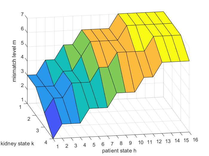
(a) Given $(h,k)$, the optimal action is to wait ($W$) if and only if the mismatch level $m$ is above the surface.

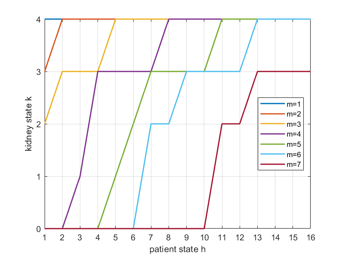
(b) Given patient state $h$, the optimal action is to wait ($W$) if and only if the kidney state $k$ is above the corresponding curve.

Figure 3: The optimal policy $d_{1}$.

The Q-function is the expected total discounted reward starting from a given state, taking a given action, and following the optimal policy thereafter. We plot in q-ex1 the Q-function, given by

$$Q(h,k,m,a)=\begin{cases}(1-{\mathcal{D}}(h,k,m))r(h,k,m)+{\mathcal{D}}(h,k,m)(c(h)+\lambda\sum_{h^{\prime}\in S_{H}}v(h^{\prime}){\mathcal{Q}}(h^{\prime}|h))&\text{if }a=T,\\ c(h)+\lambda\sum_{h^{\prime}\in S_{H}}v(h^{\prime}){\mathcal{H}}(h^{\prime}|h)&\text{if }a=W.\end{cases}$$

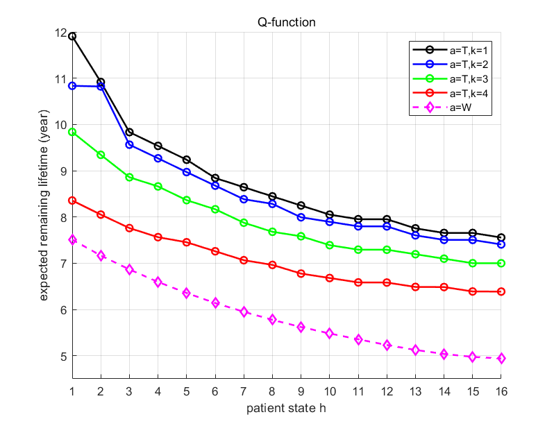
(a) $m=1$.

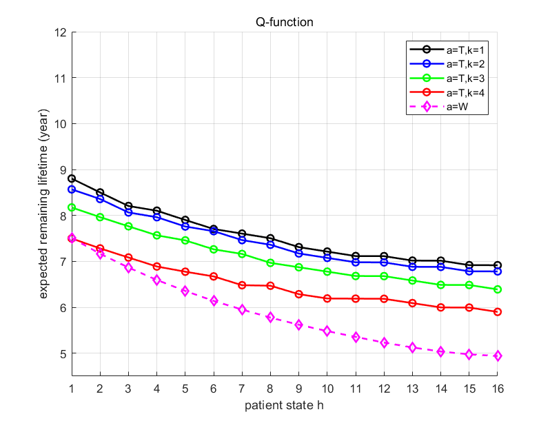
(b) $m=2$.

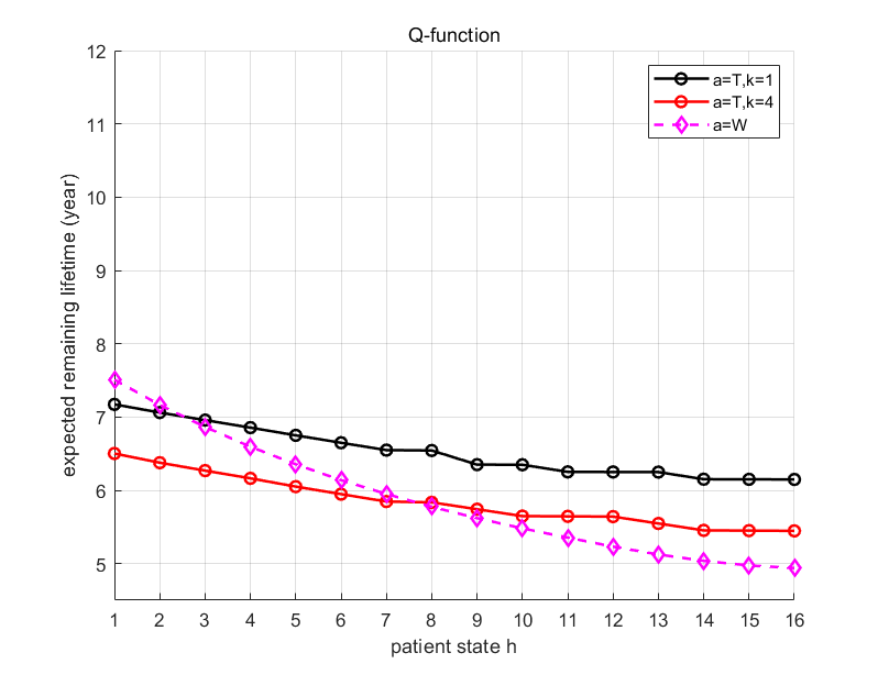
(c) $m=4$.

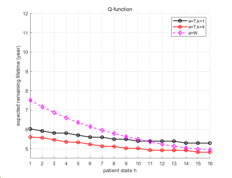
(d) $m=7$.

Figure 4: Q-function for different mismatch levels.

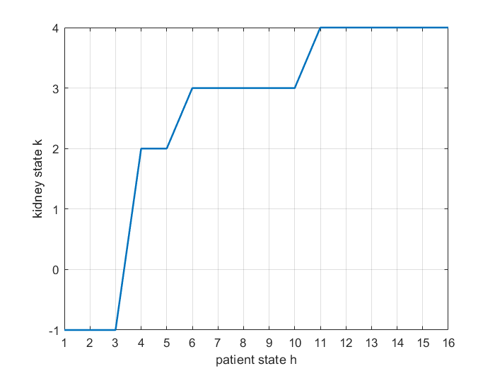
Figure 5: Policy $D$: given patient state $h$, the optimal action is to wait ($W$) if and only if the kidney state $k$ is above the curve.

Note that the value of the Q-function depends only on the patient state $h$ if the action is to wait. When the mismatch level is low, it is more beneficial to accept an offer unless it is of very low quality. As the mismatch level increases, the optimal action is to wait and then switch to transplant if the patient state $h$ is below some control limit (i.e., the patient health is worse than some threshold). For fixed mismatch level, as the patient state $h$ worsens, the optimal policy tends to accept low-quality kidneys (i.e., those with high KDPI) that are rejected at lower $h$’s. At high mismatch levels, the decision maker should choose transplant only when the patient is in severe health status (i.e., $h$ is sufficiently large).

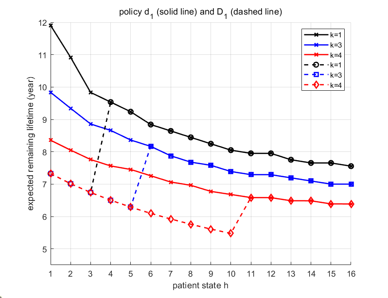
(a) $m=1$.

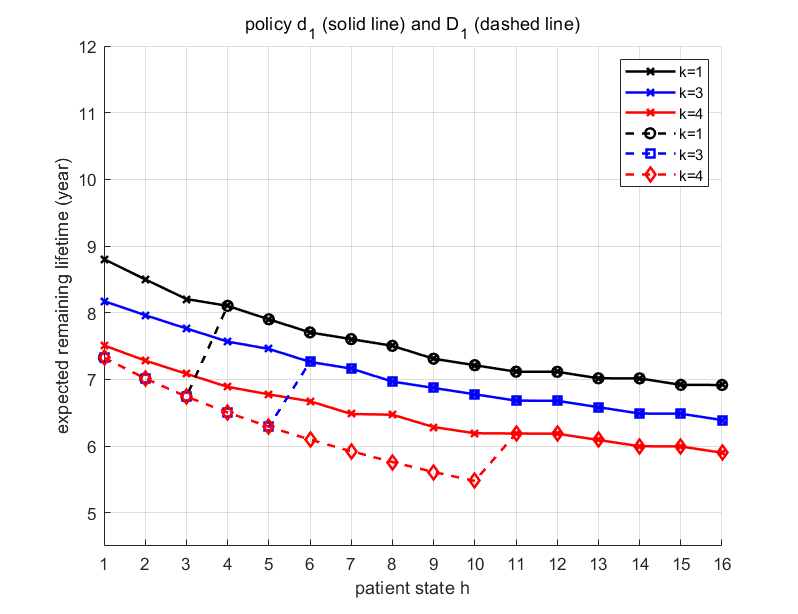
(b) $m=2$.

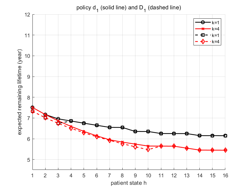
(c) $m=4$.

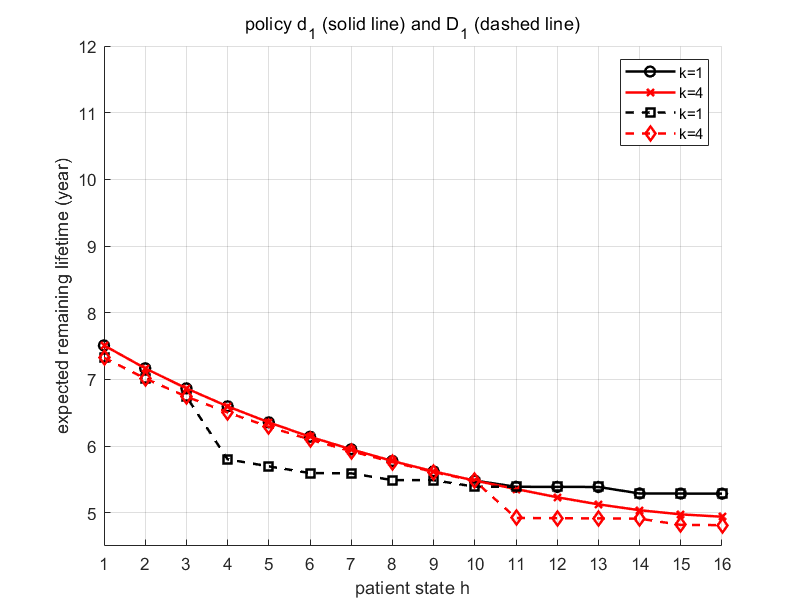
(d) $m=7$.

Figure 6: Value functions $V_{d_{1}}(h,k,m)$ and $V_{D_{1}}(h,k,m)$ for different mismatch levels. For policy $D_{1}$, fixing $m$, curves for different values of $k$ overlap with each other when $h\leq 3$ because $D_{1}$ is always $W$ for $h\leq 3$, independent of $m$. Since both $d_{1}$ and $D_{1}$ are control limit policies, fixing $k$ and $m$, if $h$ is greater than control limits of both policies, both policies choose transplant. Moreover, (8) implies that the patient state $h_{t}$ is a nondecreasing function of time, i.e., the patient health never improves. So, fixing $k$ and $m$, curves for both policies overlap when $h$ is greater than the maximum of control limits of both (patient-based) policies, which is a function of both $k$ and $m$.

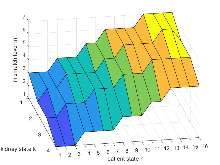
(a) Given $(h,k)$, the optimal action is to wait ($W$) if and only if the mismatch level $m$ is above the surface.

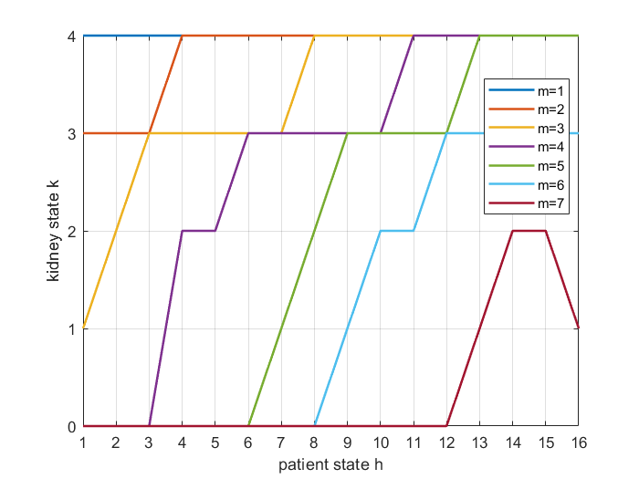
(b) Given patient state $h$, the optimal action is to wait ($W$) if and only if the kidney state $k$ is above the corresponding curve.

Figure 7: The optimal policy $d_{2}$. In the graph on the right, for mismatch level $m=7$, the optimal policy is not of control limit type.

Next, we compare with an optimal policy for an MDP model that does not include the mismatch level as a state variable, i.e., the acceptance decision making depends only on the patient and kidney states, and does not explicitly model transplantation failure or retransplantation. In the case of the latter, there is a terminal reward that is the mean over the mismatch distribution. We compute its optimal policy $D$, shown in 2d-2-ex1. Both patient-based and kidney-based control limit optimal policies exist. The control limit curve of policy $D$ lies between curves of policy $d_{1}$ for mismatch level $m=4$ and $5$. We implement the policy $D_{1}(h,k,m)=D(h,k),\forall h,k$, and $m$ in the original MDP, and compare the value functions $V_{d_{1}}(h,k,m)$ and $V_{D_{1}}(h,k,m)$ in values-m. Compared with policy $d_{1}$, when $h$ is low (i.e., the patient is healthy), policy $D_{1}$ rejects offers with low mismatch level, which would have been very beneficial to patients. As a result, policy $d_{1}$ significantly outperforms $D_{1}$ when the mismatch level $m$ is low, e.g., $m\leq 3$. At intermediate mismatch levels, the two policies behave similarly. When the mismatch level is high, e.g., $m\geq 6$, the two policies behave differently only when $h$ is high (i.e., the patient is in poor health state), where the difference of the Q-functions (i.e., the expected overall benefit) between accepting and rejecting an offer is small, as shown in q-ex1. Thus, the performances of the two policies are close when the mismatch level is intermediate to high.

Experiment 2

The optimal policy $d_{2}$ is shown in 3d-1-ex2. The kidney-based and match-based control limit optimal policies still exist, but the patient-based optimal policy for mismatch level equal to $7$ is not a control limit policy.

5 Conclusions and Future Research

We consider the problem of sequentially accepting or declining possibly incompatible kidney offers by undergoing desensitization therapies through the use of an MDP model that captures the effect of both quality and compatibility by explicitly including them as state variables. We derive structural properties of the model, specifically, characterizing control limit-type policies, including patient-based, kidney-based and match-based control limit optimal policies, by providing reasonable sufficient conditions to guarantee their existence. Numerical experiments on a stylized example based on realistic data (UNOS 2022a) illustrate that the potential gains from taking both quality and compatibility into consideration and allowing the option of accepting a mismatched kidney can be on the order of an additional year of life expectancy for a 70-year old, whose expected remaining lifetime is less than five years without kidney transplantation.

In practice, transplant surgeons make their decisions based on a variety of additional features such as demographic information and lab test results of patients and donors. Investigating the effects and relative impact of such additional information on the organ acceptance process is an interesting topic for future research.

This work was supported in part by the National Science Foundation under Grant IIS-2123684 and by AFOSR under Grant FA95502010211. The authors thank Naoru Koizumi for many useful discussions on incompatible kidney transplantation.

6 Proofs

Define

$$\begin{split}&U(h,k):=\sum_{m\in S_{M}}{\mathcal{M}}(m)V(h,k,m),~{}h\in S_{H},~{}k\in S_{K},\\ &W(h,m):=\sum_{k\in S_{k}}{\mathcal{K}}(k|h)V(h,k,m),~{}h\in S_{H},~{}m\in S_{M},\end{split}$$ (10)

which will be used in the proofs. Note that $U(h,k)$ and $W(h,m)$ have similar interpretations as $v(h)$, which can be interpreted as the expected total discounted reward when the patient state is $h$. Correspondingly, we define the following quantities associated with each iteration of the value iteration algorithm:

$$\begin{split}&U_{n}(h,k)=\sum_{m\in S_{M}}{\mathcal{M}}(m)V_{n}(h,k,m),~{}h\in S_{H},~{}k\in S_{K},\\ &W_{n}(h,m)=\sum_{k\in S_{k}}{\mathcal{K}}(k|h)V_{n}(h,k,m),~{}h\in S_{H},~{}m\in S_{M}.\end{split}$$ (11)

We begin with Lemmas 2 and 3, which are useful for proving alagoz-lemma2.

Lemma 2

(Puterman 2014) Let $\{x_{j}\}_{j\in{\mathbb{N}}},\{x_{j}^{\prime}\}_{j\in{\mathbb{N}}}$ be real-valued nonnegative sequences satisfying

$$\sum_{j=k}^{\infty}x_{j}\geq\sum_{j=k}^{\infty}x_{j}^{\prime}$$

for all $k$, with equality holding for $k=0$. Suppose $v_{j+1}\geq v_{j},~{}\forall j$, then

$$\sum_{j=0}^{\infty}v_{j}x_{j}\geq\sum_{j=0}^{\infty}v_{j}x_{j}^{\prime}.$$

puterman472col-dis immediately follows from puterman472-dis.

Lemma 3

If ${\mathcal{H}}$ is IFR and $f:{\mathbb{R}}\mapsto{\mathbb{R}}$ is nondecreasing, then

$$\sum_{h\in S_{H}}f(h){\mathcal{H}}(h|h_{1})\geq\sum_{h\in S_{H}}f(h){\mathcal{H}}(h|h_{2})$$

for any $h_{1}\geq h_{2}$.

Proof of alagoz-lemma2

Recall that $A^{*}(h,k,m)$ is the set of optimal actions at state $(h,k,m)$. Note that

$$\begin{cases}V(h,k,m)=(1-{\mathcal{D}}(h,k,m))r(h,k,m)+{\mathcal{D}}(h,k,m)(c(h)+\lambda\sum_{h^{\prime}\in S_{H}}v(h^{\prime}){\mathcal{Q}}(h^{\prime}|h))&\text{if }T\in A^{*}(h,k,m),\\ V(h,k,m)=V(h,K+1,m)&\text{if }W\in A^{*}(h,k,m),\end{cases}$$

where the second equation follows by noticing that rejecting an offer is equivalent to the offer being unavailable.

Fix $h\leq H$ and $m\in S_{M}$. Define

$$K_{T} :=\{k\in S_{K}|T\in A^{*}(h+1,k,m)\}.$$

Note that if $k\in K_{T}$, then $k\leq K$, i.e., the kidney offer is available. Then, mono-k-assump implies that ${\mathcal{K}}(k|h+1)\leq{\mathcal{K}}(k|h)$.

For $k\in K_{T}$, since $V(h,k,m)$ is nonincreasing in $h$ and $k$,

$$~{}~{}~{}~{}V(h,k,m){\mathcal{K}}(k|h)-V(h+1,k,m){\mathcal{K}}(k|h+1)$$

$$\geq V(h+1,k,m)\left({\mathcal{K}}(k|h)-{\mathcal{K}}(k|h+1)\right)$$

$$\geq V(h+1,K+1,m)\left({\mathcal{K}}(k|h)-{\mathcal{K}}(k|h+1)\right).$$

For $k\notin K_{T}$, $V(h+1,k,m)=V(h+1,K+1,m)$. Hence,

$$~{}~{}~{}~{}V(h,k,m){\mathcal{K}}(k|h)-V(h+1,k,m){\mathcal{K}}(k|h+1)$$

$$\geq V(h,K+1,m){\mathcal{K}}(k|h)-V(h+1,K+1,m){\mathcal{K}}(k|h+1)$$

$$\geq V(h+1,K+1,m)({\mathcal{K}}(k|h)-{\mathcal{K}}(k|h+1)).$$

Therefore,

$$W(h,m)-W(h+1,m) =\sum_{k\in K_{T}}(V(h,k,m){\mathcal{K}}(k|h)-V(h+1,k,m){\mathcal{K}}(k|h+1))$$

$$+\sum_{k\notin K_{T}}(V(h,k,m){\mathcal{K}}(k|h)-V(h+1,k,m){\mathcal{K}}(k|h+1))$$

$$\geq\sum_{k\in S_{K}}({\mathcal{K}}(k|h)-{\mathcal{K}}(k|h+1))V(h+1,K+1,m)$$

$$=0,$$

because $\sum_{k\in S_{K}}({\mathcal{K}}(k|h)-{\mathcal{K}}(k|h+1))=0$. It follows that

$$v(h)-v(h+1)=\sum_{m\in S_{M}}{\mathcal{M}}(m)(W(h,m)-W(h+1,m))\geq 0.~{}\blacksquare$$

Proof of mono-hk-dis

Prove by induction. Consider the value iteration algorithm (2) starting at $V_{0}(h,k,m)=0,~{}\forall h,k$, and $m$. Outline of the proof: at each step $n$, we show:

1. $V_{n}(h,k,m)$ is nonincreasing in $k$. Define

   $$K_{n}^{*}(h,m)=\max\{ k\in S_{K}\ |\ V_{n}(h,k,m)$$

   $$=(1-{\mathcal{D}}(h,k,m))r(h,k,m)+{\mathcal{D}}(h,k,m)(c(h)+\lambda\sum_{h^{\prime}\in S_{H}}v_{n-1}(h^{\prime}){\mathcal{Q}}(h^{\prime}|h))\},$$

   where we assume without loss of generality (as we show below) that

   $$\{k\in S_{K}\ |\ V_{n}(h,k,m)=(1-{\mathcal{D}}(h,k,m))r(h,k,m)+{\mathcal{D}}(h,k,m)(c(h)+\lambda\sum_{h^{\prime}\in S_{H}}v_{n}(h^{\prime}){\mathcal{Q}}(h^{\prime}|h))\}\neq\phi.$$ (12)

   We show that for fixed $h$ and $m$,

   $$~{}~{}~{}~{}V_{n}(h,k,m)$$

   $$=\begin{cases}(1-{\mathcal{D}}(h,k,m))r(h,k,m)+{\mathcal{D}}(h,k,m)(c(h)+\lambda\sum_{h^{\prime}\in S_{H}}v_{n-1}(h^{\prime}){\mathcal{Q}}(h^{\prime}|h))&\text{if }k\leq K_{n}^{*}(h,m),\\ c(h)+\lambda\sum_{h^{\prime}\in S_{H}}v_{n-1}(h^{\prime}){\mathcal{H}}(h^{\prime}|h)&\text{if }k>K_{n}^{*}(h,m).\end{cases}$$

   Then, we show that $V_{n}(h,k,m)$ is nonincreasing in $k$ on both pieces. Note that the proof of $V_{n}(h,k,m)$ being nonincreasing is trivial if (12) does not hold, because $V_{n}(h,k,m)=c(h)+\lambda\sum_{h^{\prime}\in S_{H}}v(h^{\prime}){\mathcal{H}}(h^{\prime}|h),~{}\forall k\in S_{K}$, which does not depend on $k$. From now on, we use the abbreviation $K_{n}^{*}$ for $K_{n}^{*}(h,m)$.

2. $V_{n}(h,k,m)$ and $v_{n}(h)$ are nonincreasing in $h$, where we will use Lemma 1.

Finally, the value function $V$, as the limit of the sequence $\{V_{n}\}$, is nonincreasing in both $h$ and $k$.

Initial step: by (2), for any $h$ and $m$, we have

$$V_{1}(h,k,m)=\begin{cases}\max\left((1-{\mathcal{D}}(h,k,m))r(h,k,m)+{\mathcal{D}}(h,k,m)c(h),c(h)\right)&\text{if }k=0,\cdots,K,\\ c(h)&\text{if }k=K+1.\end{cases}$$

Then,

$$~{}~{}~{}~{}~{}~{}(1-{\mathcal{D}}(h,K_{1}^{*},m))r(h,K_{1}^{*},m)+{\mathcal{D}}(h,K_{1}^{*},m)c(h)\geq c(h),$$

$$\implies(1-{\mathcal{D}}(h,K_{1}^{*},m))(r(h,K_{1}^{*},m)-c(h))\geq 0,$$

$$\implies r(h,K_{1}^{*},m)-c(h)\geq 0,$$

$$\implies r(h,k,m)-c(h)\geq 0,~{}\forall k\leq K_{1}^{*},$$

where the last step follows from transplant-reward-dis that $r(h,k,m)$ is nonincreasing in k. Therefore, $(1-{\mathcal{D}}(h,k,m))(r(h,k,m)-c(h))\geq 0,~{}\forall k\leq K_{1}^{*}$, i.e.,

$$(1-{\mathcal{D}}(h,k,m))r(h,k,m)+{\mathcal{D}}(h,k,m)c(h)\geq c(h),~{}k\leq K_{1}^{*}.$$

Thus,

$$V_{1}(h,k,m)=\begin{cases}(1-{\mathcal{D}}(h,k,m))r(h,k,m)+{\mathcal{D}}(h,k,m)c(h)&\text{if }k\leq K_{1}^{*},\\ c(h)&\text{if }k>K_{1}^{*}.\end{cases}$$

For $k\leq K_{1}^{*}$, $V_{1}(h,k,m)=(1-{\mathcal{D}}(h,k,m))(r(h,k,m)-c(h))+c(h)$. Since both $(1-{\mathcal{D}}(h,k,m))$ and $(r(h,k,m)-c(h))$ are positive and nonincreasing in $k$ for $k\leq K_{1}^{*}$, $V_{1}(h,k,m)$ is nonincreasing in $k$ for $k\leq K_{1}^{*}$. Moreover, $V_{1}(h,k,m)\geq c(h)$ for $k\leq K_{1}^{*}$. Therefore, $V_{1}(h,k,m)$ is nonincreasing in $k$.

From (2), we see that $V_{1}(h,k,m)$ takes the value of either term in the maximization. Therefore, to show $V_{1}(h,k,m)\geq V_{1}(h+1,k,m)$ for any $k$ and $m$, it suffices to consider the following four cases:

1. $V_{1}(h,k,m)=c(h),~{}V_{1}(h+1,k,m)=c(h+1)$. Proving $V_{1}(h,k,m)\geq V_{1}(h+1,k,m)$ is trivial, as $c(h)\geq c(h+1)$ by wait-reward-dis.

2. $V_{1}(h,k,m)=(1-{\mathcal{D}}(h,k,m))r(h,k,m)+{\mathcal{D}}(h,k,m)c(h),~{}V_{1}(h+1,k,m)=c(h+1)$. Then,

   $$V_{1}(h,k,m)=(1-{\mathcal{D}}(h,k,m))r(h,k,m)+{\mathcal{D}}(h,k,m)c(h)\geq c(h)\geq c(h+1)=V_{1}(h+1,k,m).$$

3. $V_{1}(h,k,m)=(1-{\mathcal{D}}(h,k,m))r(h,k,m)+{\mathcal{D}}(h,k,m)c(h),~{}V_{1}(h+1,k,m)=(1-\\ {\mathcal{D}}(h+1,k,m))r(h+1,k,m)+{\mathcal{D}}(h+1,k,m)c(h+1)$. Note that

   $$(1-{\mathcal{D}}(h,k,m))r(h,k,m)+{\mathcal{D}}(h,k,m)c(h)\geq c(h).$$

   Then,

   $$(1-{\mathcal{D}}(h,k,m))(r(h,k,m)-c(h))\geq 0\implies r(h,k,m)-c(h)\geq 0.$$

   Therefore,

   $$\begin{split}&~{}~{}~{}~{}V_{1}(h,k,m)-V_{1}(h+1,k,m)\\ &=(1-{\mathcal{D}}(h,k,m))r(h,k,m)+{\mathcal{D}}(h,k,m)c(h)-(1-{\mathcal{D}}(h+1,k,m))r(h+1,k,m)-{\mathcal{D}}(h+1,k,m)c(h+1)\\ &=(1-{\mathcal{D}}(h,k,m))r(h,k,m)+{\mathcal{D}}(h,k,m)c(h)-(1-{\mathcal{D}}(h+1,k,m))r(h+1,k,m)\\ &-{\mathcal{D}}(h,k,m)c(h+1)+({\mathcal{D}}(h,k,m)-{\mathcal{D}}(h+1,k,m))c(h+1)\\ &\geq(1-{\mathcal{D}}(h,k,m))r(h,k,m)+{\mathcal{D}}(h,k,m)c(h)-(1-{\mathcal{D}}(h+1,k,m))r(h+1,k,m)\\ &-{\mathcal{D}}(h,k,m)c(h+1)+({\mathcal{D}}(h,k,m)-{\mathcal{D}}(h+1,k,m))r(h,k,m)\\ &=(1-{\mathcal{D}}(h+1,k,m))(r(h,k,m)-r(h+1,k,m))+{\mathcal{D}}(h,k,m)(c(h)-c(h+1))\\ &\geq 0,\end{split}$$ (13)

   where the first inequality follows from the fact that ${\mathcal{D}}(h,k,m)\leq{\mathcal{D}}(h+1,k,m)$ and $r(h,k,m)\geq c(h)\geq c(h+1)$, and the last inequality follows from Assumptions 2 and 1.

4. $V_{1}(h,k,m)=c(h),~{}V_{1}(h+1,k,m)=(1-{\mathcal{D}}(h+1,k,m))r(h+1,k,m)+{\mathcal{D}}(h+1,k,m)c(h+1)$. Note that

   $$(1-{\mathcal{D}}(h+1,k,m))r(h+1,k,m)+{\mathcal{D}}(h+1,k,m)c(h+1)\geq c(h+1).$$

   Then,

   $$(1-{\mathcal{D}}(h+1,k,m))(r(h+1,k,m)-c(h+1))\geq 0\implies r(h+1,k,m)-c(h+1)\geq 0\implies c(h+1)\leq r(h,k,m).$$

   Notice that $V_{1}(h,k,m)\geq(1-{\mathcal{D}}(h,k,m))r(h,k,m)+{\mathcal{D}}(h,k,m)c(h)$. Using the same argument as (13), we have $V_{1}(h,k,m)\geq V_{1}(h+1,k,m)$.

Thus, $V_{1}(h,k,m)$ is nonincreasing in $h$. alagoz-lemma2 implies that $v_{1}(h)$ is nonincreasing in $h$.

Induction step: suppose that $V_{n}(h,k,m)$ is nonincreasing in both $h$ and $k$, and $v_{n}(h)$ is nonincreasing in $h$. By (2),

$$\begin{split}&V_{n+1}(h,k,m)=\max\begin{pmatrix}(1-{\mathcal{D}}(h,k,m))r(h,k,m)+{\mathcal{D}}(h,k,m)(c(h)+\lambda\sum_{h^{\prime}\in S_{H}}v_{n}(h^{\prime}){\mathcal{Q}}(h^{\prime}|h))\\ c(h)+\lambda\sum_{h^{\prime}\in S_{H}}v_{n}(h^{\prime}){\mathcal{H}}(h^{\prime}|h)\end{pmatrix},\\ &V_{n+1}(h,K+1,m)=c(h)+\lambda\sum_{h^{\prime}\in S_{H}}v_{n}(h^{\prime}){\mathcal{H}}(h^{\prime}|h),\end{split}$$

$\\ ~{}\forall h\in S_{H},~{}m\in S_{M},~{}k<K+1$. Then, for any $h$ and $m$,

$$~{}~{}~{}~{}(1-{\mathcal{D}}(h,K_{n}^{*},m))r(h,K_{n}^{*},m)+{\mathcal{D}}(h,K_{n}^{*},m)(c(h)+\lambda\sum_{h^{\prime}\in S_{H}}v_{n}(h^{\prime}){\mathcal{Q}}(h^{\prime}|h))$$

$$=(1-{\mathcal{D}}(h,K_{n}^{*},m))\left(r(h,K_{n}^{*},m)-c(h)-\lambda\sum_{h^{\prime}\in S_{H}}v_{n}(h^{\prime}){\mathcal{Q}}(h^{\prime}|h)\right)+c(h)+\lambda\sum_{h^{\prime}\in S_{H}}v_{n}(h^{\prime}){\mathcal{Q}}(h^{\prime}|h)$$

$$\geq c(h)+\lambda\sum_{h^{\prime}\in S_{H}}v_{n}(h^{\prime}){\mathcal{H}}(h^{\prime}|h).$$

It follows that

$$(1-{\mathcal{D}}(h,K_{n}^{*},m))\left(r(h,K_{n}^{*},m)-c(h)-\lambda\sum_{h^{\prime}\in S_{H}}v_{n}(h^{\prime}){\mathcal{Q}}(h^{\prime}|h)\right)\geq\lambda\sum_{h^{\prime}\in S_{H}}v_{n}(h^{\prime})({\mathcal{H}}(h^{\prime}|h)-{\mathcal{Q}}(h^{\prime}|h))\geq 0,$$

where the last inequality follows from diffifr-dis that ${\mathcal{H}}\succeq_{st}{\mathcal{Q}}$ and puterman472col-dis. Since $r(h,k,m)$ is nonincreasing in $k$,

$$r(h,k,m)-c(h)-\lambda\sum_{h^{\prime}\in S_{H}}v_{n}(h^{\prime}){\mathcal{Q}}(h^{\prime}|h)\geq 0,~{}\forall k\leq K_{n}^{*}.$$

Since ${\mathcal{D}}(h,k,m)$ is nondecreasing in $k$, $\forall k\leq K_{n}^{*}$,

$$(1-{\mathcal{D}}(h,k,m))\left(r(h,k,m)-c(h)-\lambda\sum_{h^{\prime}\in S_{H}}v_{n}(h^{\prime}){\mathcal{Q}}(h^{\prime}|h)\right)\geq\lambda\sum_{h^{\prime}\in S_{H}}v_{n}(h^{\prime})({\mathcal{H}}(h^{\prime}|h)-{\mathcal{Q}}(h^{\prime}|h)),$$

i.e.,

$$(1-{\mathcal{D}}(h,k,m))r(h,k,m)+{\mathcal{D}}(h,k,m)(c(h)+\lambda\sum_{h^{\prime}\in S_{H}}v_{n}(h^{\prime}){\mathcal{Q}}(h^{\prime}|h))\geq c(h)+\lambda\sum_{h^{\prime}\in S_{H}}v_{n}(h^{\prime}){\mathcal{H}}(h^{\prime}|h).$$

Therefore,

$$\begin{cases}V_{n+1}(h,k,m)=(1-{\mathcal{D}}(h,k,m))r(h,k,m)+{\mathcal{D}}(h,k,m)(c(h)+\lambda\sum_{h^{\prime}\in S_{H}}v_{n}(h^{\prime}){\mathcal{Q}}(h^{\prime}|h))&\text{if }k\leq K_{n}^{*},\\ V_{n+1}(h,k,m)=c(h)+\lambda\sum_{h^{\prime}\in S_{H}}v_{n}(h^{\prime}){\mathcal{H}}(h^{\prime}|h)&\text{if }k>K_{n}^{*}.\end{cases}$$

Moreover, when $k\leq K_{n}^{*}$,

$$~{}~{}~{}~{}(1-{\mathcal{D}}(h,k,m))r(h,k,m)+{\mathcal{D}}(h,k,m)(c(h)+\lambda\sum_{h^{\prime}\in S_{H}}v_{n}(h^{\prime}){\mathcal{Q}}(h^{\prime}|h))$$

$$=(1-{\mathcal{D}}(h,k,m))\left(r(h,k,m)-c(h)-\lambda\sum_{h^{\prime}\in S_{H}}v_{n}(h^{\prime}){\mathcal{Q}}(h^{\prime}|h)\right)+c(h)+\lambda\sum_{h^{\prime}\in S_{H}}v_{n}(h^{\prime}){\mathcal{Q}}(h^{\prime}|h),$$

where both $(1-{\mathcal{D}}(h,k,m))$ and $\left(r(h,k,m)-c(h)-\lambda\sum_{h^{\prime}\in S_{H}}v_{n}(h^{\prime}){\mathcal{Q}}(h^{\prime}|h)\right)$ are positive and nonincreasing in $k$, so $(1-{\mathcal{D}}(h,k,m))r(h,k,m)+{\mathcal{D}}(h,k,m)(c(h)+\lambda\sum_{h^{\prime}\in S_{H}}v_{n}(h^{\prime}){\mathcal{Q}}(h^{\prime}|h))$ is nonincreasing in $k$ for $k\leq K_{n}^{*}$. Moreover, $(1-{\mathcal{D}}(h,k,m))r(h,k,m)+{\mathcal{D}}(h,k,m)(c(h)+\lambda\sum_{h^{\prime}\in S_{H}}v_{n}(h^{\prime}){\mathcal{Q}}(h^{\prime}|h))\geq c(h)+\lambda\sum_{h^{\prime}\in S_{H}}v_{n}(h^{\prime}){\mathcal{H}}(h^{\prime}|h)$ for $k\leq K_{n}^{*}$. Therefore, $V_{n+1}(h,k,m)$ is nonincreasing in $k$.

To show $V_{n+1}(h,k,m)\geq V_{n+1}(h+1,k,m)$ for any $k$ and $m$, as above, it suffices to consider the following four cases:

1. $V_{n+1}(h,k,m)=c(h)+\lambda\sum_{h^{\prime}\in S_{H}}v_{n}(h^{\prime}){\mathcal{H}}(h^{\prime}|h),~{}V_{n+1}(h+1,k,m)=c(h+1)+\lambda\sum_{h^{\prime}\in S_{H}}v_{n}(h^{\prime}){\mathcal{H}}(h^{\prime}|h+1)$. By wait-reward-dis, $c(h)\geq c(h+1)$. By markovifr-dis, puterman472col-dis and $v_{n}(h)$ being nonincreasing, $\sum_{h^{\prime}\in S_{H}}v_{n}(h^{\prime}){\mathcal{H}}(h^{\prime}|h)\geq\sum_{h^{\prime}\in S_{H}}v_{n}(h^{\prime}){\mathcal{H}}(h^{\prime}|h+1)$. So, $V_{n+1}(h,k,m)\geq V_{n+1}(h+1,k,m)$.

2. $V_{n+1}(h,k,m)=(1-{\mathcal{D}}(h,k,m))r(h,k,m)+{\mathcal{D}}(h,k,m)(c(h)+\lambda\sum_{h^{\prime}\in S_{H}}v_{n}(h^{\prime}){\mathcal{Q}}(h^{\prime}|h)),~{}V_{n+1}(h+1,k,m)=c(h+1)+\lambda\sum_{h^{\prime}\in S_{H}}v_{n}(h^{\prime}){\mathcal{H}}(h^{\prime}|h+1))$. Then,

   $$V_{n+1}(h,k,m)\geq c(h)+\lambda\sum_{h^{\prime}\in S_{H}}v_{n}(h^{\prime}){\mathcal{H}}(h^{\prime}|h)\geq c(h+1)+\lambda\sum_{h^{\prime}\in S_{H}}v_{n}(h^{\prime}){\mathcal{H}}(h^{\prime}|h+1)=V_{n+1}(h+1,k,m),$$

   where the second inequality follows from the same argument as the first case.

3. $V_{n+1}(h,k,m)=(1-{\mathcal{D}}(h,k,m))r(h,k,m)+{\mathcal{D}}(h,k,m)(c(h)+\lambda\sum_{h^{\prime}\in S_{H}}v_{n}(h^{\prime}){\mathcal{Q}}(h^{\prime}|h)),~{}V_{n+1}(h+1,k,m)=(1-{\mathcal{D}}(h+1,k,m))r(h+1,k,m)+{\mathcal{D}}(h+1,k,m)(c(h+1)+\lambda\sum_{h^{\prime}\in S_{H}}v_{n}(h^{\prime}){\mathcal{Q}}(h^{\prime}|h+1))$. Note that ${\mathbb{E}}g((h,k,m),T)=(1-{\mathcal{D}}(h,k,m))r(h,k,m)+{\mathcal{D}}(h,k,m)c(h),~{}\forall h,k,$ and $m$. Then,

   $$\begin{split}&~{}~{}~{}~{}V_{n+1}(h,k,m)-V_{n+1}(h+1,k,m)\\ &={\mathbb{E}}g((h,k,m),T)+{\mathcal{D}}(h,k,m)\lambda\sum_{h^{\prime}\in S_{H}}v_{n}(h^{\prime}){\mathcal{Q}}(h^{\prime}|h)\\ &-{\mathbb{E}}g((h+1,k,m),T)-{\mathcal{D}}(h+1,k,m)\lambda\sum_{h^{\prime}\in S_{H}}v_{n}(h^{\prime}){\mathcal{Q}}(h^{\prime}|h+1)\\ &={\mathbb{E}}g((h,k,m),T)-{\mathbb{E}}g((h+1,k,m),T)+({\mathcal{D}}(h,k,m)-{\mathcal{D}}(h+1,k,m))\lambda\sum_{h^{\prime}\in S_{H}}v_{n}(h^{\prime}){\mathcal{Q}}(h^{\prime}|h)\\ &+{\mathcal{D}}(h+1,k,m)\lambda\sum_{h^{\prime}\in S_{H}}v_{n}(h^{\prime})({\mathcal{Q}}(h^{\prime}|h)-{\mathcal{Q}}(h^{\prime}|h+1))\\ &\geq{\mathbb{E}}g((h,k,m),T)-{\mathbb{E}}g((h+1,k,m),T)+({\mathcal{D}}(h,k,m)-{\mathcal{D}}(h+1,k,m))\lambda\sum_{h^{\prime}\in S_{H}}v_{n}(h^{\prime}){\mathcal{Q}}(h^{\prime}|h),\end{split}$$ (14)

   where the last inequality follows from puterman472col-dis, markovifr-dis and $v_{n}(h)$ being nonincreasing. Note that $V_{n+1}(h,k,m)\geq c(h)+\lambda\sum_{h^{\prime}\in S_{H}}v_{n}(h^{\prime}){\mathcal{H}}(h^{\prime}|h)$, i.e.,

   $$~{}~{}~{}~{}(1-{\mathcal{D}}(h,k,m))\left(r(h,k,m)-c(h)-\lambda\sum_{h^{\prime}\in S_{H}}v_{n}(h^{\prime}){\mathcal{Q}}(h^{\prime}|h)\right)$$

   $$\geq\lambda\sum_{h^{\prime}\in S_{H}}v_{n}(h^{\prime})({\mathcal{H}}(h^{\prime}|h)-{\mathcal{Q}}(h^{\prime}|h))$$

   $$\geq 0,$$

   where the last inequality follows from puterman472col-dis and diffifr-dis. So,

   $$r(h,k,m)-c(h)\geq\lambda\sum_{h^{\prime}\in S_{H}}v_{n}(h^{\prime}){\mathcal{Q}}(h^{\prime}|h).$$

   Since ${\mathcal{D}}(h,k,m)-{\mathcal{D}}(h+1,k,m)\leq 0$, by (14),

   $$~{}~{}~{}~{}V_{n+1}(h,k,m)-V_{n+1}(h+1,k,m)$$

   $$\geq{\mathbb{E}}g((h,k,m),T)-{\mathbb{E}}g((h+1,k,m),T)+({\mathcal{D}}(h,k,m)-{\mathcal{D}}(h+1,k,m))(r(h,k,m)-c(h))$$

   $$=(1-{\mathcal{D}}(h,k,m))r(h,k,m)+{\mathcal{D}}(h,k,m)c(h)-(1-{\mathcal{D}}(h+1,k,m))r(h+1,k,m)-{\mathcal{D}}(h+1,k,m)c(h+1)$$

   $$+({\mathcal{D}}(h,k,m)-{\mathcal{D}}(h+1,k,m))(r(h,k,m)-c(h))$$

   $$=(1-{\mathcal{D}}(h+1,k,m))(r(h,k,m)-r(h+1,k,m))+{\mathcal{D}}(h+1,k,m)(c(h)-c(h+1))$$

   $$\geq 0,$$

   where the last inequality follows from Assumptions 2 and 1.

4. $V_{n+1}(h,k,m)=c(h)+\lambda\sum_{h^{\prime}\in S_{H}}v_{n}(h^{\prime}){\mathcal{H}}(h^{\prime}|h),~{}V_{n+1}(h+1,k,m)=(1-{\mathcal{D}}(h+1,k,m))r(h+1,k,m)+{\mathcal{D}}(h+1,k,m)(c(h+1)+\lambda\sum_{h^{\prime}\in S_{H}}v_{n}(h^{\prime}){\mathcal{Q}}(h^{\prime}|h+1))$. Note that

   $$~{}~{}~{}~{}(1-{\mathcal{D}}(h+1,k,m))r(h+1,k,m)+{\mathcal{D}}(h+1,k,m)(c(h+1)+\lambda\sum_{h^{\prime}\in S_{H}}v_{n}(h^{\prime}){\mathcal{Q}}(h^{\prime}|h+1))$$

   $$\geq c(h+1)+\lambda\sum_{h^{\prime}\in S_{H}}v_{n}(h^{\prime}){\mathcal{H}}(h^{\prime}|h+1)).$$

   Then,

   $$~{}~{}~{}~{}(1-{\mathcal{D}}(h+1,k,m))\left(r(h+1,k,m)-c(h+1)-\lambda\sum_{h^{\prime}\in S_{H}}v_{n}(h^{\prime}){\mathcal{Q}}(h^{\prime}|h+1)\right)$$

   $$\geq\lambda\sum_{h^{\prime}\in S_{H}}v_{n}(h^{\prime})({\mathcal{H}}(h^{\prime}|h+1)-{\mathcal{Q}}(h^{\prime}|h+1))$$

   $$\geq 0,$$

   where the last inequality follows from puterman472col-dis, diffifr-dis and $v_{n}$ being nonincreasing. So,

   $$c(h+1)+\lambda\sum_{h^{\prime}\in S_{H}}v_{n}(h^{\prime}){\mathcal{Q}}(h^{\prime}|h+1)\leq r(h+1,k,m).$$ (15)

   Then,

   $$~{}~{}~{}~{}V_{n+1}(h,k,m)-V_{n+1}(h+1,k,m)$$

   $$={\mathbb{E}}g((h,k,m),T)+{\mathcal{D}}(h,k,m)\lambda\sum_{h^{\prime}\in S_{H}}v_{n}(h^{\prime}){\mathcal{Q}}(h^{\prime}|h)$$

   $$-{\mathbb{E}}g((h+1,k,m),T)-{\mathcal{D}}(h+1,k,m)\lambda\sum_{h^{\prime}\in S_{H}}v_{n}(h^{\prime}){\mathcal{Q}}(h^{\prime}|h+1)$$

   $$={\mathbb{E}}g((h,k,m),T)-{\mathbb{E}}g((h+1,k,m),T)+{\mathcal{D}}(h,k,m)\lambda\sum_{h^{\prime}\in S_{H}}v_{n}(h^{\prime})({\mathcal{Q}}(h^{\prime}|h)-{\mathcal{Q}}(h^{\prime}|h+1))$$

   $$-({\mathcal{D}}(h+1,k,m)-{\mathcal{D}}(h,k,m))\lambda\sum_{h^{\prime}\in S_{H}}v_{n}(h^{\prime}){\mathcal{Q}}(h^{\prime}|h+1)$$

   $$\geq={\mathbb{E}}g((h,k,m),T)-{\mathbb{E}}g((h+1,k,m),T)-({\mathcal{D}}(h+1,k,m)-{\mathcal{D}}(h,k,m))\lambda\sum_{h^{\prime}\in S_{H}}v_{n}(h^{\prime}){\mathcal{Q}}(h^{\prime}|h+1)$$

   $$\geq{\mathbb{E}}g((h,k,m),T)-{\mathbb{E}}g((h+1,k,m),T)+({\mathcal{D}}(h,k,m)-{\mathcal{D}}(h+1,k,m)))(r(h+1,k,m)-c(h+1))$$

   $$=(1-{\mathcal{D}}(h,k,m))r(h,k,m)+{\mathcal{D}}(h,k,m)c(h)-(1-{\mathcal{D}}(h+1,k,m))r(h+1,k,m)-{\mathcal{D}}(h+1,k,m)c(h+1)$$

   $$+({\mathcal{D}}(h,k,m)-{\mathcal{D}}(h+1,k,m)))(r(h+1,k,m)-c(h+1))$$

   $$=(1-{\mathcal{D}}(h,k,m))(r(h,k,m)-r(h+1,k,m))+{\mathcal{D}}(h,k,m)(c(h)-c(h+1))$$

   $$\geq 0,$$

   where the first inequality follows from puterman472col-dis, diffifr-dis and $v_{n}$ being nonincreasing, and the second inequality follows from (15).

Therefore, $V_{n+1}(h,k,m)$ is nonincreasing in $h$. alagoz-lemma2 implies that $v_{n+1}$ is nonincreasing in $h$. Finally, function $V$, as the limit of sequence $\{V_{n}\}$, is nonincreasing in both $h$ and $k$, and alagoz-lemma2 implies that $v$ is nonincreasing in $h$. $\blacksquare$

Proof of Theorems 3 and 4

To show the existence of the match-based control limit policy, it is equivalent to show that $T\in A^{*}(h,k,m+1)$ implies $T\in A^{*}(h,k,m)$ for any $h,k,m$, where $A^{*}(h,k,m)$ is the set of optimal actions at state $(h,k,m)$. Assume that $T\in A^{*}(h,k,m+1)$, then

$$V(h,k,m+1) =(1-{\mathcal{D}}(h,k,m+1))r(h,k,m+1)+{\mathcal{D}}(h,k,m+1)(c(h)+\lambda\sum_{h^{\prime}\in S_{H}}v(h^{\prime}){\mathcal{Q}}(h^{\prime}|h))$$

$$\geq c(h)+\lambda\sum_{h^{\prime}\in S_{H}}v(h^{\prime}){\mathcal{H}}(h^{\prime}|h),$$

i.e.,

$$~{}~{}~{}~{}(1-{\mathcal{D}}(h,k,m+1)(r(h,k,m+1)-c(h))$$

$$\geq(1-{\mathcal{D}}(h,k,m+1))\lambda\sum_{h^{\prime}\in S_{H}}v(h^{\prime}){\mathcal{H}}(h^{\prime}|h))+{\mathcal{D}}(h,k,m+1)\lambda\sum_{h^{\prime}\in S_{H}}v(h^{\prime})({\mathcal{H}}(h^{\prime}|h)-{\mathcal{Q}}(h^{\prime}|h)),$$

i.e.,

$$~{}~{}~{}~{}(1-{\mathcal{D}}(h,k,m+1)(r(h,k,m+1)-c(h)-\lambda\sum_{h^{\prime}\in S_{H}}v(h^{\prime}){\mathcal{H}}(h^{\prime}|h))$$

$$\geq{\mathcal{D}}(h,k,m+1)\lambda\sum_{h^{\prime}\in S_{H}}v(h^{\prime})({\mathcal{H}}(h^{\prime}|h)-{\mathcal{Q}}(h^{\prime}|h))$$

$$\geq 0,$$

where the last inequality follows from puterman472col-dis, diffifr-dis and $v$ being nonincreasing. So, if $T\in A^{*}(h,k,m+1)$,

$$r(h,k,m+1)-c(h)-\lambda\sum_{h^{\prime}\in S_{H}}v(h^{\prime}){\mathcal{H}}(h^{\prime}|h)\geq 0.$$ (16)

Since ${\mathcal{D}}(h,k,m)$ is nondecreasing in $m$ and $r(h,k,m)$ is nonincreasing in $m$, we have

$$~{}~{}~{}~{}(1-{\mathcal{D}}(h,k,m)(r(h,k,m)-c(h)-\lambda\sum_{h^{\prime}\in S_{H}}v(h^{\prime}){\mathcal{H}}(h^{\prime}|h))$$

$$\geq{\mathcal{D}}(h,k,m)\lambda\sum_{h^{\prime}\in S_{H}}v(h^{\prime})({\mathcal{H}}(h^{\prime}|h)-{\mathcal{Q}}(h^{\prime}|h)),$$

i.e.,

$$V(h,k,m) =(1-{\mathcal{D}}(h,k,m))r(h,k,m)+{\mathcal{D}}(h,k,m)(c(h)+\lambda\sum_{h^{\prime}\in S_{H}}v(h^{\prime}){\mathcal{Q}}(h^{\prime}|h))$$

$$\geq c(h)+\lambda\sum_{h^{\prime}\in S_{H}}v(h^{\prime}){\mathcal{H}}(h^{\prime}|h).$$

Therefore, $T\in A^{*}(h,k,m)$. The proof of kidney-based-dis is exactly the same (by showing $T\in A^{*}(h,k+1,m)\implies T\in A^{*}(h,k,m)$) and is omitted. $\blacksquare$

Proof of mono-m-dis

If $m\geq M^{*}(h,k)$, it is optimal to choose $W$, and $V(h,k,m)=c(h)+\lambda\sum_{h^{\prime}\in S_{H}}v(h^{\prime}){\mathcal{H}}(h^{\prime}|h)$, as a function of $m$, is constant.

If $m<M^{*}(h,k)$, $T\in A^{*}(h,k,m)$ and

$$V(h,k,m)= (1-{\mathcal{D}}(h,k,m))r(h,k,m)+{\mathcal{D}}(h,k,m)(c(h)+\lambda\sum_{h^{\prime}\in S_{H}}v(h^{\prime}){\mathcal{Q}}(h^{\prime}|h))$$

$$\geq c(h)+\lambda\sum_{h^{\prime}\in S_{H}}v(h^{\prime}){\mathcal{H}}(h^{\prime}|h).$$

In particular, $V(h,k,M^{*}(h,k)-1)\geq V(h,k,M^{*}(h,k))$. From (16), we know that $r(h,k,m)-c(h)-\lambda\sum_{h^{\prime}\in S_{H}}v(h^{\prime}){\mathcal{H}}(h^{\prime}|h)\geq 0$ for $m<M^{*}(h,k)$.

Since $\sum_{h^{\prime}\in S_{H}}v(h^{\prime}){\mathcal{H}}(h^{\prime}|h)\geq\sum_{h^{\prime}\in S_{H}}v(h^{\prime}){\mathcal{Q}}(h^{\prime}|h)$ (follows from puterman472col-dis, diffifr-dis and $v$ being nonincreasing), we have $r(h,k,m)-c(h)-\lambda\sum_{h^{\prime}\in S_{H}}v(h^{\prime}){\mathcal{Q}}(h^{\prime}|h)\geq 0$ for $m<M^{*}(h,k)$.

Rewrite

$$V(h,k,m) =(1-{\mathcal{D}}(h,k,m))\left(r(h,k,m)-c(h)-\lambda\sum_{h^{\prime}\in S_{H}}v(h^{\prime}){\mathcal{Q}}(h^{\prime}|h)\right)$$

$$+\left(c(h)+\lambda\sum_{h^{\prime}\in S_{H}}v(h^{\prime}){\mathcal{Q}}(h^{\prime}|h)\right).$$

Since ${\mathcal{D}}(h,k,m)$ is nondecreasing in $m$ and $r(h,k,m)$ is nonincreasing in $m$, $V(h,k,m)$ is nonincreasing in $m$ for $m<M^{*}(h,k)$. Thus, $V(h,k,m)$ is nonincreasing in $m$. $\blacksquare$

Proof of mono-limit-1-dis

When proving match-based-dis, we showed that for any $k,h$, $T\in a(h,k,m+1)$ implies that $T\in a(h,k,m)$, i,e, $k<K^{*}(h,m+1)$ implies that $k<K^{*}(h,m)$. Hence, $K^{*}(h,m+1)\leq K^{*}(h,m)$. Similarly, we can argue that $M^{*}(h,k+1)\leq M^{*}(h,k)$. The last two statements follow from monotonicity. $\blacksquare$

schaefer-lemma3 is provided in Alagoz et al. (2007b).

Lemma 4

Suppose transition probability function $P(\cdot|\cdot):S\times S\mapsto[0,1]$ on state space $S=\{1,\cdots,n\}$ is IFR. If function $f:{\mathbb{R}}\mapsto{\mathbb{R}}_{+}$ is nonincreasing, the following inequalities hold: for $i=1,\cdots,n,~{}j=1,\cdots,n-1$,

1. $\sum_{i\leq j}(P(i|j)-P(i|j+1))f(i)\geq\sum_{i\leq j}(P(i|j)-P(i|j+1))f(j)$;

2. $\sum_{i>j}(P(i|j)-P(i|j+1))f(i)\geq\sum_{i>j}(P(i|j)-P(i|j+1))f(j+1)$.

Proof of health-based-dis

It is equivalent to show that $T\in A^{*}(h,k,m)$ implies that $T\in A^{*}(h+1,k,m)$ for any $h,k,$ and $m$. Fix $h\leq H,~{}k\leq K$. Prove by contradiction: suppose that $T\in A^{*}(h,k,m)$ but $A^{*}(h+1,k,m)=W$. Since $T\in A^{*}(h,m,k)$, we have

$$\begin{split}V(h,k,m)&={\mathbb{E}}g((h,k,m),T)+{\mathcal{D}}(h,k,m)\lambda\sum_{h^{\prime}\in S_{H}}v(h^{\prime}){\mathcal{Q}}(h^{\prime}|h)\\ &\geq c(h)+\lambda\sum_{h^{\prime}\in S_{H}}v(h^{\prime}){\mathcal{H}}(h^{\prime}|h).\end{split}$$ (17)

Since $A^{*}(h+1,m,k)=W$, the following strict inequality holds:

$$\begin{split}&~{}~{}~{}~{}{\mathbb{E}}g((h+1,k,m),T)+{\mathcal{D}}(h+1,k,m)\lambda\sum_{h^{\prime}\in S_{H}}v(h^{\prime}){\mathcal{Q}}(h^{\prime}|h+1)\\ &<c(h+1)+\lambda\sum_{h^{\prime}\in S_{H}}v(h^{\prime}){\mathcal{H}}(h^{\prime}|h+1).\end{split}$$ (18)

Subtracting (18) from (17),

$$~{}~{}~{}~{}{\mathbb{E}}g((h,k,m),T)+{\mathcal{D}}(h,k,m)\lambda\sum_{h^{\prime}\in S_{H}}v(h^{\prime}){\mathcal{Q}}(h^{\prime}|h)$$

$$-{\mathbb{E}}g((h+1,k,m),T)-{\mathcal{D}}(h+1,k,m)\lambda\sum_{h^{\prime}\in S_{H}}v(h^{\prime}){\mathcal{Q}}(h^{\prime}|h+1)$$

$$>c(h)-c(h+1)+\lambda\sum_{h^{\prime}\in S_{H}}v(h^{\prime}){\mathcal{H}}(h^{\prime}|h)-\lambda\sum_{h^{\prime}\in S_{H}}v(h^{\prime}){\mathcal{H}}(h^{\prime}|h+1).$$

Since ${\mathcal{D}}(h+1,k,m)\geq{\mathcal{D}}(h,k,m)$ (desenfail-dis),

$$\begin{split}&~{}~{}~{}~{}{\mathbb{E}}g((h,k,m),T)-{\mathbb{E}}g((h+1,k,m),T)\\ &>c(h)-c(h+1)+{\mathcal{D}}(h,k,m)\lambda\sum_{h^{\prime}\in S_{H}}v(h^{\prime})({\mathcal{Q}}(h^{\prime}|h+1)-{\mathcal{Q}}(h^{\prime}|h))\\ &+\lambda\sum_{h^{\prime}\in S_{H}}v(h^{\prime})\left({\mathcal{H}}(h^{\prime}|h)-{\mathcal{H}}(h^{\prime}|h+1)\right)\\ &\geq{\mathcal{D}}(h,k,m)\lambda\sum_{h^{\prime}\in S_{H}}v(h^{\prime})({\mathcal{Q}}(h^{\prime}|h+1)-{\mathcal{Q}}(h^{\prime}|h))\\ &+\lambda\sum_{h^{\prime}\in S_{H}}v(h^{\prime})\left({\mathcal{H}}(h^{\prime}|h)-{\mathcal{H}}(h^{\prime}|h+1)\right)\\ &={\mathcal{D}}(h,k,m)\lambda\sum_{h^{\prime}\in S_{H}}v(h^{\prime})({\mathcal{Q}}(h^{\prime}|h+1)-{\mathcal{H}}(h^{\prime}|h+1)-({\mathcal{Q}}(h^{\prime}|h)-{\mathcal{H}}(h^{\prime}|h)))\\ &+\lambda(1-{\mathcal{D}}(h,k,m))\sum_{h^{\prime}\in S_{H}}v(h^{\prime})\left({\mathcal{H}}(h^{\prime}|h)-{\mathcal{H}}(h^{\prime}|h+1)\right)\\ &\geq\lambda(1-{\mathcal{D}}(h,k,m))\sum_{h^{\prime}\in S_{H}}v(h^{\prime})\left({\mathcal{H}}(h^{\prime}|h)-{\mathcal{H}}(h^{\prime}|h+1)\right),\end{split}$$ (19)

where the second inequality follows from wait-reward-dis that $c(h)\geq c(h+1)$; to prove the last inequality, it is enough to notice that

$$~{}~{}~{}~{}\sum_{h^{\prime}\in S_{H}}v(h^{\prime})({\mathcal{Q}}(h^{\prime}|h+1)-{\mathcal{H}}(h^{\prime}|h+1)-({\mathcal{Q}}(h^{\prime}|h)-{\mathcal{H}}(h^{\prime}|h)))$$

$$=\sum_{h^{\prime}\in S_{H}}v(h^{\prime})({\mathcal{Q}}(h^{\prime}|h+1)+{\mathcal{H}}(h^{\prime}|h)-({\mathcal{H}}(h^{\prime}|h+1)+{\mathcal{Q}}(h^{\prime}|h)))$$

$$\geq 0$$

because of puterman472-dis, h-based-con3 and $v$ being nonincreasing.

From (LABEL:proof-mono-dis-3), it follows that

$$\begin{split}&~{}~{}~{}~{}{\mathbb{E}}g((h,k,m),T)-{\mathbb{E}}g((h+1,k,m),T)\\ &>\lambda(1-{\mathcal{D}}(h,k,m))\sum_{h^{\prime}\in S_{H}}v(h^{\prime})\left({\mathcal{H}}(h^{\prime}|h)-{\mathcal{H}}(h^{\prime}|h+1)\right)\\ &=\lambda(1-{\mathcal{D}}(h,k,m))\left(\sum_{h^{\prime}=1}^{h}v(h^{\prime})\left({\mathcal{H}}(h^{\prime}|h)-{\mathcal{H}}(h^{\prime}|h+1)\right)+\sum_{h^{\prime}=h+1}^{H}v(h^{\prime})\left({\mathcal{H}}(h^{\prime}|h)-{\mathcal{H}}(h^{\prime}|h+1)\right)\right)\end{split}$$ (20)

(note that $v(H+1)=0$). Since $v$ is nonincreasing, by applying both parts of schaefer-lemma3 to each of the sums in (LABEL:proof-mono-dis-4), respectively, we have

$$~{}~{}~{}~{}{\mathbb{E}}g((h,k,m),T)-{\mathbb{E}}g((h+1,k,m),T)$$

$$>\lambda(1-{\mathcal{D}}(h,k,m))\left(v(h)\sum_{h^{\prime}=1}^{h}\left({\mathcal{H}}(h^{\prime}|h)-{\mathcal{H}}(h^{\prime}|h+1)\right)+v(h+1)\sum_{h^{\prime}=h+1}^{H}\left({\mathcal{H}}(h^{\prime}|h)-{\mathcal{H}}(h^{\prime}|h+1)\right)\right)$$

$$=\lambda(1-{\mathcal{D}}(h,k,m))v(h)\left(1-\sum_{h^{\prime}=h+1}^{H}{\mathcal{H}}(h^{\prime}|h)-{\mathcal{H}}(H+1|h)-\left(1-\sum_{h^{\prime}=h+1}^{H}{\mathcal{H}}(h^{\prime}|h+1)-{\mathcal{H}}(H+1|h+1)\right)\right)$$

$$+\lambda(1-{\mathcal{D}}(h,k,m))v(h+1)\sum_{h^{\prime}=h+1}^{H}\left({\mathcal{H}}(h^{\prime}|h)-{\mathcal{H}}(h^{\prime}|h+1)\right)$$

$$=\lambda(1-{\mathcal{D}}(h,k,m))(v(h)-v(h+1))\sum_{h^{\prime}=h+1}^{H}\left({\mathcal{H}}(h^{\prime}|h+1)-{\mathcal{H}}(h^{\prime}|h)\right)$$

$$+\lambda(1-{\mathcal{D}}(h,k,m))v(h)({\mathcal{H}}(H+1|h+1)-{\mathcal{H}}(H+1|h)).$$

By h-based-con1, $\sum_{h^{\prime}=h+1}^{H}\left({\mathcal{H}}(h^{\prime}|h+1)-{\mathcal{H}}(h^{\prime}|h)\right)\geq 0$. Therefore,

$${\mathbb{E}}g((h,k,m),T)-{\mathbb{E}}g((h+1,k,m),T)>\lambda(1-{\mathcal{D}}(h,k,m))v(h)\left({\mathcal{H}}(H+1|h+1)-{\mathcal{H}}(H+1|h)\right)$$ (21)

From h-based-con2 and (21), we have

$$v(h)<{\mathbb{E}}g((h+1,k,m),T).$$

Since ${\mathbb{E}}g((h+1,k,m),T)\leq V(h+1,k,m)$, we obtain $v(h)<V(h+1,k,m)$. By (18), $V(h+1,k,m)=c(h+1)+\lambda\sum_{h^{\prime}\in S_{H}}v_{n}(h^{\prime}){\mathcal{H}}(h^{\prime}|h+1)=V(h+1,K+1,m)$. Then, by the monotonicity of $V(h,k,m)$ in both $h$ and $k$,

$$v(h)<V(h+1,k,m)=V(h+1,K+1,m)\leq V(h,K+1,m)\leq v(h),$$

where the last inequality follows from the fact that $V(h,K+1,m)\leq V(h,k,m),~{}\forall k,m$, which is a contradiction. Therefore, $T\in A^{*}(h,k,m)$ implies that $T\in A^{*}(h+1,k,m)$. $\blacksquare$

Proof of diff-avai

Prove by induction. Suppose that we solve $\Pi_{1}$ and $\Pi_{2}$ simultaneously using value iteration (2) with $V_{0}^{1}(h,k,m)=V_{0}^{2}(h,k,m)=0,~{}\forall h,k,$ and $m$. Let $V^{i}_{j}$ be the value function of $\Pi_{i},~{}i=1,2$ at the $j^{th}$ iteration.

Initial step: at the first iteration,

$$V_{1}^{1}(h,k,m)=V_{1}^{2}(h,k,m)=\begin{cases}\max\left((1-{\mathcal{D}}(h,k,m))r(h,k,m)+{\mathcal{D}}(h,k,m)c(h),c(h)\right)&\text{if }k\leq K,\\ c(h)&\text{if }k=K.\end{cases}$$

Thus, we have $U_{1}^{1}(h,k)=U_{1}^{2}(h,k),~{}\forall h,k.$ As shown in the proof of mono-hk-dis, $V_{1}^{1}(h,k,m)$ and $V_{1}^{2}(h,k,m)$ are nonincreasing in $h$ and $k$. Hence, $U_{1}^{1}(h,k)$ and $U_{1}^{2}(h,k)$ are nonincreasing in $h$ and $k$ as well.

Since ${\mathcal{K}}_{1}\succeq_{st}{\mathcal{K}}_{2}$, by puterman472-dis,

$$\sum_{k\in S_{K}}\left(U_{1}^{1}(h,k){\mathcal{K}}_{1}(k|h)-U_{1}^{2}(h,k){\mathcal{K}}_{2}(k|h)\right)=\sum_{k\in S_{K}}U_{1}^{1}(h,k)\left({\mathcal{K}}_{1}(k|h)-{\mathcal{K}}_{2}(k|h)\right)\geq 0,~{}\forall h\in S_{H},$$

i.e., $v^{1}_{1}(h)\geq v^{2}_{1}(h),~{}\forall h\in S_{H}$.

Induction step: now assume that $v^{1}_{n}(h)\geq v^{2}_{n}(h)$ and $V_{n}^{1}(h,k,m)\geq V_{n}^{2}(h,k,m)$ for all $h,k,$ and $m$. We want to show $V_{n+1}^{1}(h,k,m)\geq V_{n+1}^{2}(h,k,m)$ for all $h,k,$ and $m$. By inspecting (2), we note that it suffices to show

$$\begin{split}\sum_{h^{\prime}\in S_{H}}v^{1}_{n}(h^{\prime}){\mathcal{H}}(h^{\prime}|h)\geq\sum_{h^{\prime}\in S_{H}}v^{2}_{n}(h^{\prime}){\mathcal{H}}(h^{\prime}|h),\end{split}$$ (22)

$$\begin{split}\sum_{h^{\prime}\in S_{H}}v^{1}_{n}(h^{\prime}){\mathcal{Q}}(h^{\prime}|h)\geq\sum_{h^{\prime}\in S_{H}}v^{2}_{n}(h^{\prime}){\mathcal{Q}}(h^{\prime}|h).\end{split}$$ (23)

We will show (22), and (23) can be proved in the same way. We write $v_{n}^{i}(h)=\sum_{k\in S_{k}}U_{n}^{i}(h,k){\mathcal{K}}_{i}(k|h),~{}i=1,2$. Since $V_{n}^{1}(h,k,m)\geq V_{n}^{2}(h,k,m)$ for all $h,k,$ and $m$, $U_{n}^{1}(h,k)\geq U_{n}^{2}(h,k)$ for all $h$ and $k$. Then,

$$~{}~{}~{}~{}\sum_{h^{\prime}\in S_{H}}v^{1}_{n}(h^{\prime}){\mathcal{H}}(h^{\prime}|h)-\sum_{h^{\prime}\in S_{H}}v^{2}_{n}(h^{\prime}){\mathcal{H}}(h^{\prime}|h)$$

$$=\sum_{h^{\prime}\in S_{H}}\left(\sum_{k\in S_{k}}U_{n}^{1}(h^{\prime},k){\mathcal{K}}_{1}(k|h^{\prime})\right){\mathcal{H}}(h^{\prime}|h)-\sum_{h^{\prime}\in S_{H}}\left(\sum_{k\in S_{k}}U_{n}^{2}(h^{\prime},k){\mathcal{K}}_{2}(k|h^{\prime})\right){\mathcal{H}}(h^{\prime}|h)$$

$$=\sum_{h^{\prime}\in S_{H}}{\mathcal{H}}(h^{\prime}|h)\sum_{k\in S_{K}}\left(U_{n}^{1}(h^{\prime},k){\mathcal{K}}_{1}(k|h^{\prime})-U_{n}^{2}(h^{\prime},k){\mathcal{K}}_{2}(k|h^{\prime})\right)$$

$$\geq\sum_{h^{\prime}\in S_{H}}{\mathcal{H}}(h^{\prime}|h)\sum_{k\in S_{K}}\left(U_{n}^{2}(h^{\prime},k){\mathcal{K}}_{1}(k|h^{\prime})-U_{n}^{2}(h^{\prime},k){\mathcal{K}}_{2}(k|h^{\prime})\right).$$

As shown in the proof of mono-hk-dis, both $V_{n}^{1}(h,k,m)$ and $V_{n}^{2}(h,k,m)$ are nonincreasing in $k$ for any $n$. Thus, both $U_{n}^{1}(h,k)$ and $U_{n}^{2}(h,k)$ are nonincreasing in $k$. Since ${\mathcal{K}}_{1}\succeq_{st}{\mathcal{K}}_{2}$, by puterman472-dis,

$$\sum_{k\in S_{K}}\left(U_{n}^{2}(h^{\prime},k){\mathcal{K}}_{1}(k|h^{\prime})-U_{n}^{2}(h^{\prime},k){\mathcal{K}}_{2}(k|h^{\prime})\right)\geq 0,~{}\forall h^{\prime}\in S_{H}.$$

Therefore, $\sum_{h^{\prime}\in S_{H}}v^{1}_{n}(h^{\prime}){\mathcal{H}}(h^{\prime}|h)\geq\sum_{h^{\prime}\in S_{H}}v^{2}_{n}(h^{\prime}){\mathcal{H}}(h^{\prime}|h)$.

It follows that $V_{n+1}^{1}(h,k,m)\geq V_{n+1}^{2}(h,k,m),~{}\forall h,k,$ and $m$. Then, $U_{n+1}^{1}(h,k)\geq U_{n+1}^{2}(h,k)$ for all $h$ and $k$, and

$$v^{1}_{n+1}(h)-v^{2}_{n+1}(h) =\sum_{k\in S_{K}}\left(U_{n+1}^{1}(h,k){\mathcal{K}}_{1}(k|h)-U_{n+1}^{2}(h,k){\mathcal{K}}_{2}(k|h)\right)$$

$$\geq\sum_{k\in S_{K}}\left(U_{n+1}^{2}(h,k){\mathcal{K}}_{1}(k|h)-U_{n+1}^{2}(h,k){\mathcal{K}}_{2}(k|h)\right)$$

$$\geq 0,~{}\forall h\in S_{H},$$

where the second inequality follows from puterman472-dis and ${\mathcal{K}}_{1}\succeq_{st}{\mathcal{K}}_{2}$. Therefore, $v^{1}_{n}(h)\geq v^{2}_{n}(h)$ and $V_{n}^{1}(h,k,m)\geq V_{n}^{2}(h,k,m),~{}\forall n$. Taking $n\rightarrow\infty$, we have $v^{1}(h)\geq v^{2}(h)$ and $V^{1}(h,k,m)\geq V^{2}(h,k,m),~{}\forall h,k,$ and $m$. $\blacksquare$

To prove diff-trans, we need the following lemma from Alagoz et al. (2007b).

Lemma 5

Suppose transition probability functions $P(\cdot|\cdot),Q(\cdot|\cdot)$ on state space $S=\{1,\cdots,n\}$ satisfying $P\succeq_{st}Q$. Then the following inequalities hold for any function nonincreasing $f:{\mathbb{R}}\mapsto{\mathbb{R}}_{+}$: for $i,j=1,\cdots,n$,

1. $\sum_{j\leq i}(P(j|i)-Q(j|i))f(j)\geq\sum_{j\leq i}(P(j|i)-Q(j|i))f(i)$.

2. $\sum_{j>i}(P(j|i)-Q(j|i))f(j)\geq\sum_{j>i}(P(j|i)-Q(j|i))f(i+1)$.

Proof of diff-trans

Prove by induction. Suppose that we solve $\Pi_{1}$ and $\Pi_{2}$ simultaneously using value iteration (2) with $V_{0}^{1}(h,k,m)=V_{0}^{2}(h,k,m)=0,~{}\forall h,k,$ and $m$. Let $V^{i}_{j}$ be the value function of $\Pi_{i},~{}i=1,2$ at the $j^{th}$ iteration.

Initial step: at the first iteration,

$$V_{1}^{1}(h,k,m)=V_{1}^{2}(h,k,m)=\begin{cases}\max\left((1-{\mathcal{D}}(h,k,m))r(h,k,m)+{\mathcal{D}}(h,k,m)c(h),c(h)\right)&\text{if }k\leq K,\\ c(h)&\text{if }k=K.\end{cases}$$

Thus, $v^{1}_{1}(h)=v^{2}_{1}(h),\forall h$.

Induction step: assume that $V_{n}^{1}(h,k,m)\geq V_{n}^{2}(h,k,m),~{}v_{n}^{1}(h)\geq v_{n}^{2}(h),~{}\forall h,k,$ and $m$. We want to show $V_{n+1}^{1}(h,k,m)\geq V_{n+1}^{2}(h,k,m),~{}v_{n+1}^{1}(h)\geq v_{n+1}^{2}(h),~{}\forall h,k,$ and $m$. By inspecting (2), we note that it suffices to show

$$\begin{split}\sum_{h^{\prime}\in S_{H}}v^{1}_{n}(h^{\prime}){\mathcal{H}}_{1}(h^{\prime}|h)\geq\sum_{h^{\prime}\in S_{H}}v^{2}_{n}(h^{\prime}){\mathcal{H}}_{2}(h^{\prime}|h),\end{split}$$ (24)

$$\begin{split}\sum_{h^{\prime}\in S_{H}}v^{1}_{n}(h^{\prime}){\mathcal{Q}}_{1}(h^{\prime}|h)\geq\sum_{h^{\prime}\in S_{H}}v^{2}_{n}(h^{\prime}){\mathcal{Q}}_{2}(h^{\prime}|h).\end{split}$$ (25)

We will show (24), and (25) can be proved in the same way. We have

$$\begin{split}&~{}~{}~{}~{}\sum_{h^{\prime}\in S_{H}}v^{1}_{n}(h^{\prime}){\mathcal{H}}_{1}(h^{\prime}|h)-\sum_{h^{\prime}\in S_{H}}v^{2}_{n}(h^{\prime}){\mathcal{H}}_{2}(h^{\prime}|h)\\ &\geq\sum_{h^{\prime}\leq h}v^{2}_{n}(h^{\prime}){\mathcal{H}}_{1}(h^{\prime}|h)+\sum_{h^{\prime\prime}>h}v^{2}_{n}(h^{\prime\prime}){\mathcal{H}}_{1}(h^{\prime\prime}|h)-\sum_{h^{\prime}\leq h}v^{2}_{n}(h^{\prime}){\mathcal{H}}_{2}(h^{\prime}|h)-\sum_{h^{\prime\prime}>h}v^{2}_{n}(h^{\prime\prime}){\mathcal{H}}_{2}(h^{\prime\prime}|h)\\ &=\sum_{h^{\prime}\leq h}v^{2}_{n}(h^{\prime})\left({\mathcal{H}}_{1}(h^{\prime}|h)-{\mathcal{H}}_{2}(h^{\prime}|h)\right)+\sum_{h^{\prime\prime}>h}v^{2}_{n}(h^{\prime\prime})\left({\mathcal{H}}_{1}(h^{\prime\prime}|h)-{\mathcal{H}}_{2}(h^{\prime\prime}|h)\right)\\ &\geq v^{2}_{n}(h)\sum_{h^{\prime}\leq h}\left({\mathcal{H}}_{1}(h^{\prime}|h)-{\mathcal{H}}_{2}(h^{\prime}|h)\right)+v^{2}_{n}(h+1)\sum_{h^{\prime\prime}>h}\left({\mathcal{H}}_{1}(h^{\prime\prime}|h)-{\mathcal{H}}_{2}(h^{\prime\prime}|h)\right)\\ &=\left(v^{2}_{n}(h)-v^{2}_{n}(h+1)\right)\sum_{h^{\prime}\leq h}\left({\mathcal{H}}_{1}(h^{\prime}|h)-{\mathcal{H}}_{2}(h^{\prime}|h)\right)\\ &\geq 0,\end{split}$$ (26)

where the first inequality follows from the induction assumption that $v^{1}_{n}(h^{\prime})\geq v^{2}_{n}(h^{\prime}),~{}\forall h^{\prime}$, the second inequality follows from schaefer-lemma4 and $v_{n}^{2}$ being nonincreasing (shown in the proof of mono-hk-dis), and the second equality follows from the fact that

$$\sum_{h^{\prime}\leq h}\left({\mathcal{H}}_{1}(h^{\prime}|h)-{\mathcal{H}}_{2}(h^{\prime}|h)\right)+\sum_{h^{\prime\prime}>h}\left({\mathcal{H}}_{1}(h^{\prime\prime}|h)-{\mathcal{H}}_{2}(h^{\prime\prime}|h)\right)=0.$$

The last equality holds because $v^{2}_{n}(h)\geq v^{2}_{n}(h+1)$ and $\sum_{h^{\prime}\leq h}\left({\mathcal{H}}_{1}(h^{\prime}|h)-{\mathcal{H}}_{2}(h^{\prime}|h)\right)\geq 0$, which follows from ${\mathcal{H}}_{1}\succeq_{st}{\mathcal{H}}_{2}$. Therefore, $V_{n+1}^{1}(h,k,m)\geq V_{n+1}^{2}(h,k,m),~{}\forall h,k,m$. Since $\Pi_{1}$ and $\Pi_{2}$ have the same ${\mathcal{K}}$ and ${\mathcal{M}}$, $v_{n+1}^{1}(h)\geq v_{n+1}^{2}(h)$. Taking $n\rightarrow\infty$, we have $v^{1}(h)\geq v^{2}(h)$ and $V^{1}(h,k,m)\geq V^{2}(h,k,m),~{}\forall h,k,$ and $m$. $\blacksquare$

7 Selection of Parameters in Numerical Experiments

7.1 Definition of States and Transition Law

The raw EPTS score is computed by the following formula (UNOS 2022d):

raw EPTS $$=(0.047-0.015\times{\mathbf{1}}\{\text{diabetes}\})\times(\text{age}-25)^{+}$$

$$+(0.398-0.237\times{\mathbf{1}}\{\text{diabetes}\})\times\text{number of prior organ transplantations}$$

$$+(0.315-0.099\times{\mathbf{1}}\{\text{diabetes}\})\times\log(\text{years on dialysis +1})$$

$$+(0.130-0.348\times{\mathbf{1}}\{\text{diabetes}\})\times{\mathbf{1}}\{\text{no dialysis}\}$$

$$+1.262\times{\mathbf{1}}\{\text{diabetes}\}$$

where ${\mathbf{1}}\{\cdot\}$ is the indicator function of an event and $x^{+}:=\max(x,0)$. Patients with lower EPTS scores are expected to have longer time of graft function from high-longevity kidneys, compared to patients with higher EPTS scores. The raw EPTS is converted to an EPTS score (ranging from $0$ to $100$) using the EPTS mapping table. An online calculator can be found at the UNOS website (UNOS 2022b).

To define the probability of death, i.e., ${\mathcal{H}}(H+1|h)$, at each patient state, we find in the latest UNOS data report (UNOS 2022a) that deaths per 100 patient years for kidney registrations during waiting is $6.91$ for patients over $65$, thus, the probability of death in a year is roughly $0.0691$, and therefore, we use $0.035$ as the probability of death for each epoch. We want to choose ${\mathcal{H}}(H+1|h),~{}\forall h$ to keep the arithmetic average of ${\mathcal{H}}(H+1|h)$ over $S_{H}$ close to $0.035$. Since older patients are more likely to die, we take ${\mathcal{H}}(H+1|h)$ to be increasing in $h$.

If the patient chooses to wait and is alive, their state transition law is deterministic as shown in EPTS-evolve (transition probability function ${\mathcal{H}}$ can be defined accordingly). If the patient experiences a transplantation failure, we define the state transition law according to the change in their EPTS score, as shown in Table 3 (transition probability function ${\mathcal{Q}}$ can be defined accordingly). It is easy to check that Assumptions 4, 5, and 7, but not Assumption 9, are satisfied. However, Assumption 9 would hold if we directly define patient state by EPTS score, as Table 3 indicates that there is a larger drop in EPTS score when patients with lower EPTS scores experience a transplant failure, compared with patients with higher EPTS scores.

patient state $h$	EPTS score
1	53
2	60
3	67
4	72
5	76
6	80
7	83
8	86
9	89
10	91
11	93
12	94
13	96
14	97
15	98
16	$99$ or greater
17	death

Table 2: Definition of patient state $h$ and corresponding EPTS scores.

pre-transplant EPTS score	patient state $h$	post-transplant EPTS score	patient state $h$
53	1	79	6
60	2	85	8
67	3	89	9
72	4	92	10
76	5	95	12
80	6	97	13
83	7	98	14
86 or greater	8 or greater	99 or greater	16

Table 3: Patient state transition law after a transplantation failure.

We use the kidney donor profile index (KDPI) score to represent the kidney state $k$ and assume that kidney state $\{k_{n}\}_{n=1}^{\infty}$ form an i.i.d. sequence of random variables, independent of both patient state and mismatch level. KDPI, a scalar that combines ten donor factors including clinical parameters and demographics, is used in the kidney allocation system to measure the quality of deceased donor kidneys (UNOS 2022c). KDPI score ranges from $0$ to $100$. The average waiting time for a kidney offer is $2.13$ years according to the latest UNOS report (UNOS 2022a), so we assume that the patient’s waiting time is a geometric random variable with mean $2.13$ years. Therefore, the probability that a patient gets an offer is $0.2347$ for each epoch (six months). We define four types of kidney state by their KDPI ranges. ${\mathcal{K}}$, the distribution of the kidney state, is obtained from UNOS (2022a) and shown in Table 4. mono-k-assump holds, because we assume that the distribution of kidney state is independent of patient state.

KDPI range	kidney state $k$	probability ($\%$)
0-20	1	4.91
21-34	2	3.23
35-85	3	12.06
86-100	4	3.47
Not available	5	76.53

Table 4: The distribution of kidney state.

The distribution of mismatch level ${\mathcal{M}}$ in deceased donor kidney transplantation, also obtained from UNOS (2022a), is given in Table 5.

mismatch level $m$	probability ($\%$)
1	4.92
2	1.04
3	1.92
4	14.37
5	28.06
6	32.54
7	14.14

Table 5: The distribution of mismatch level ${\mathcal{M}}$.

We assume in sec4 that the probability of a transplantation failure depends only on $k$ and $m$, not on $h$, and we denote it by ${\mathcal{D}}(k,m)$. We use the six-month post-transplantation graft failure rate to represent ${\mathcal{D}}(k,m)$. For deceased donor kidney transplantation, the six-month post-transplantation graft survival rate is $97.1\%$ for perfect match, and $94.7\%$ for non-perfect match (UNOS 2022a).

mismatch level $m$	six month graft survival probability ($\%$)
$m=1$	97.1
$m>1$	94.7

Table 6: Six-month post-transplantation graft survival rate for zero and nonzero mismatch levels (UNOS 2022a).

For deceased donor kidney transplantation, the six-month post-transplantation graft survival rate for different KDPI ranges is given in Table 7.

KDPI range	kidney state $k$	graft survival probability ($\%$)
0-20	1	97.1
21-34	2	95.1
35-85	3	94.1
86-100	4	91.6

Table 7: Six-month post-transplantation graft survival rate for different KDPI ranges (UNOS 2022a).

${\mathcal{D}}(k,m)$	$m=1$	$m>1$
$k=1$	1.7	4.1
$k=2$	3.7	6.1
$k=3$	4.7	7.1
$k=4$	7.3	9.5

Table 8: The probability ($\%$) of a transplantation failure ${\mathcal{D}}(k,m)$.

Mismatch level $m$	relative risk
1	0.9
2	1
3	1.1
4	1.2
5	1.3
6	1.4
7	1.6

Table 9: Relative risk for different HLA-mismatch levels.

For each KDPI range, we assume that the six-month post-transplantation graft survival rate for $m=1$ and $m>1$ have the same ratio as Table 6, and the six-month graft survival rate for each KDPI range in Table 7 is equal to the arithmetic average of the survival rate for $m=1$ and $m>1$. Then, the probability of a transplantation failure ${\mathcal{D}}(k,m)$ is given in Table 8. We verify that desenfail-dis holds for ${\mathcal{D}}$ specified in succ-trans.

7.2 Rewards

	0-20	21-34	35-85	86-100
53-54	87.5	86.8	83.85	76.55
59-60	86	85.3	82.2	74.65
67-68	83.75	83.05	79.75	72
71-72	82.4	81.75	78.35	70.5
75-76	80.95	80.3	76.8	68.85
79-80	79.3	78.6	75.05	67.05
83-84	77.6	76.8	73.05	65.15
85-86	76.65	75.85	71.05	64.05
89-90	74.45	73.8	69.85	61.95
91-92	73.65	72.7	68.7	60.8
93-94	72.6	71.6	67.45	59.6
95-96	71.5	70.4	66.15	58.4
97	70.6	69.5	65.2	57.5
98	70	68.8	64.5	56.8
99 or greater	69.4	68.2	63.8	56.2

Table 10: The five-year post-transplantation patient survival rate ($\%$).

	0-20	21-34	35-85	86-100
53-54	12	11	10	8.5
59-60	11	11	9.5	8.2
67-68	9.9	9.7	9	7.9
71-72	9.6	9.4	8.8	7.7
75-76	9.3	9.1	8.5	7.6
79-80	8.9	8.8	8.3	7.4
83-84	8.7	8.5	8	7.2
85-86	8.5	8.4	7.8	7.1
89-90	8.3	8.1	7.7	6.9
91-92	8.1	8	7.5	6.8
93-94	8	7.9	7.4	6.7
95-96	7.8	7.7	7.3	6.6
97	7.7	7.6	7.2	6.6
98	7.7	7.6	7.1	6.5
99 or greater	7.6	7.5	7.1	6.5

Table 11: Expected post-transplantation patient survival time for $m=1$.

	0-20	21-34	35-85	86-100
53-54	6	5.9	5.8	5.5
59-60	5.9	5.9	5.8	55
67-68	5.8	5.8	5.7	5.4
71-72	5.8	5.7	5.6	5.3
75-76	5.7	5.7	5.6	5.3
79-80	5.6	5.6	5.5	5.2
83-84	5.6	5.6	5.4	5.1
85-86	5.5	5.5	5.3	5.1
89-90	5.5	5.4	5.3	5
91-92	5.4	5.4	5.3	5
93-94	5.4	5.4	5.2	4.9
95-96	5.4	5.3	5.2	4.9
97	5.3	5.3	5.1	4.8
98	5.3	5.2	5.1	4.8
99 or greater	5.3	5.2	5.1	4.8

Table 12: Expected post-transplantation patient survival time for $m=7$.

We set the intermediate reward to be $0.5$ years, i.e., $c(h)=0.5,~{}\forall h$. We use the expected post-transplantation survival time to represent the post-transplantation reward $r(h,k,m)$. We assume that the patient post-transplantation survival time is a Poisson random variable (with unit to be a year). If we know the five-year post-transplantation patient survival rate, we can approximate the expected post-transplantation survival time with the mean of the corresponding Poisson random variable. For each EPTS-KDPI pair, the five-year post-transplantation patient survival rate can be found in Bae et al. (2019). For each EPTS-KDPI range in Table 10, the five-year post-transplantation survival rate is approximated by the arithmetic average of survival rate at endpoints of the EPTS range with KDPI score to be the median of the KDPI range.

To compute the post-transplantation reward, we also need to take into consideration the effect of mismatch level. We use the relative risk (Opelz and Döhler 2007) to measure relative contribution of HLA to the five-year patient survival rate.

We set mismatch level $m=5$ to be the reference and use the relative risk measure shown in Table 9. Given EPTS score, KDPI score, and mismatch level, the five-year patient survival rate is obtained by the corresponding probability in Table 10 divided by the relative risk in Table 9.

EPTS-KDPI-survival-0 and Table 12 show the expected post-transplantation patient survival time for $m=1$ and $m=7$, respectively. When the EPTS or KDPI score is low, the expected post-transplantation survival time is much longer for $m=1$, compared with $m=7$. When the EPTS or KDPI score is high, the effect of mismatch level is less obvious. Assumptions 1 and 2 hold with the reward functions we used.

References

- Ahn and Hornberger (1996) Ahn JH, Hornberger JC (1996) Involving patients in the cadaveric kidney transplant allocation process: A decision-theoretic perspective. Management Science 42(5):629–641.
- Aimaretti and Arze (2016) Aimaretti LA, Arze S (2016) Preemptive renal transplantation—the best treatment option for terminal chronic renal failure. Transplantation Proceedings, volume 48, 609–611 (Elsevier).
- Alagoz et al. (2010) Alagoz O, Hsu H, Schaefer AJ, Roberts MS (2010) Markov decision processes: A tool for sequential decision making under uncertainty. Medical Decision Making 30(4):474–483.
- Alagoz et al. (2004) Alagoz O, Maillart LM, Schaefer AJ, Roberts MS (2004) The optimal timing of living-donor liver transplantation. Management Science 50(10):1420–1430.
- Alagoz et al. (2007a) Alagoz O, Maillart LM, Schaefer AJ, Roberts MS (2007a) Choosing among living-donor and cadaveric livers. Management Science 53(11):1702–1715.
- Alagoz et al. (2007b) Alagoz O, Maillart LM, Schaefer AJ, Roberts MS (2007b) Determining the acceptance of cadaveric livers using an implicit model of the waiting list. Operations Research 55(1):24–36.
- Bae et al. (2019) Bae S, Massie AB, Thomas AG, Bahn G, Luo X, Jackson KR, Ottmann SE, Brennan DC, Desai NM, Coresh J, Segev DL, Wang GJ (2019) Who can tolerate a marginal kidney? predicting survival after deceased donor kidney transplant by donor–recipient combination. American Journal of Transplantation 19(2):425–433.
- Batun et al. (2018) Batun S, Schaefer AJ, Bhandari A, Roberts MS (2018) Optimal liver acceptance for risk-sensitive patients. Service Science 10(3):320–333.
- Bendersky and David (2016) Bendersky M, David I (2016) Deciding kidney-offer admissibility dependent on patients’ lifetime failure rate. European Journal of Operational Research 251(2):686–693.
- Bertsekas (2020) Bertsekas DP (2020) Dynamic Programming and Optimal Control, 4th edition, Volume I (Athena Scientific).
- Clayton and Coates (2017) Clayton PA, Coates PT (2017) Are sensitized patients better off with a desensitization transplant or waiting on dialysis? Kidney International 91(6):1266–1268.
- David and Yechiali (1985) David I, Yechiali U (1985) A time-dependent stopping problem with application to live organ transplants. Operations Research 33(3):491–504.
- Fan et al. (2020) Fan W, Zong Y, Kumar S (2020) Optimal treatment of chronic kidney disease with uncertainty in obtaining a transplantable kidney: An MDP-based approach. Annals of Operations Research 316(11):269–302.
- Fiorentino et al. (2021) Fiorentino M, Gallo P, Giliberti M, Colucci V, Schena A, Stallone G, Gesualdo L, Castellano G (2021) Management of patients with a failed kidney transplant: what should we do? Clinical Kidney Journal 14(1):98–106.
- Husain et al. (2019) Husain SA, King KL, Pastan S, Patzer RE, Cohen DJ, Radhakrishnan J, Mohan S (2019) Association between declined offers of deceased donor kidney allograft and outcomes in kidney transplant candidates. JAMA Network Open 2(8):e1910312–e1910312.
- Kaufman et al. (2017) Kaufman D, Schaefer AJ, Roberts MS (2017) Living-donor liver transplantation timing under ambiguous health state transition probabilities. Available at SSRN 3003590 .
- Konvalinka and Tinckam (2015) Konvalinka A, Tinckam K (2015) Utility of HLA antibody testing in kidney transplantation. Journal of the American Society of Nephrology 26(7):1489–1502.
- Koo and Yang (2015) Koo TY, Yang J (2015) Current progress in ABO-incompatible kidney transplantation. Kidney Research and Clinical Practice 34(3):170–179.
- Kuppachi and Axelrod (2020) Kuppachi S, Axelrod DA (2020) Desensitization strategies: Is it worth it? Transplant International 33(3):251–259.
- Mahawar and Bal (2004) Mahawar KK, Bal AM (2004) Role of hla matching in liver transplant. Transplantation 78(2):643.
- Marfo et al. (2011) Marfo K, Lu A, Ling M, Akalin E (2011) Desensitization protocols and their outcome. Clinical Journal of the American Society of Nephrology 6(4):922–936.
- Opelz and Döhler (2007) Opelz G, Döhler B (2007) Effect of human leukocyte antigen compatibility on kidney graft survival: comparative analysis of two decades. Transplantation 84(2):137–143.
- Puterman (2014) Puterman ML (2014) Markov Decision Processes: Discrete Stochastic Dynamic Programming (John Wiley & Sons).
- Ren et al. (2022) Ren X, Fu M, Marcus SI (2022) Stochastic control for organ donations: A review. Systems & Control Letters Submitted.
- Ross (1996) Ross SM (1996) Stochastic Processes (Wiley New York), second edition.
- UNOS (2022a) UNOS (2022a) Eliminate use of DSA and region from kidney allocation: One year post-implementation monitoring report. URL https://unos.org/news/1-yr-kidney-data-report-transplant-increases/, (accessed: 07.19.2022).
- UNOS (2022b) UNOS (2022b) EPTS calculator. URL https://optn.transplant.hrsa.gov/data/allocation-calculators/epts-calculator/, (accessed: 07.19.2022).
- UNOS (2022c) UNOS (2022c) Kidney donor profile index (KDPI) guide for clinicians. URL https://optn.transplant.hrsa.gov/professionals/by-topic/guidance/kidney-donor-profile-index-kdpi-guide-for-clinicians, (accessed: 07.19.2022).
- UNOS (2022d) UNOS (2022d) Learn about EPTS. URL https://optn.transplant.hrsa.gov/data/allocation-calculators/epts-calculator/learn-about-epts/, (accessed: 07.19.2022).
- UNOS (2022e) UNOS (2022e) View data source. URL https://optn.transplant.hrsa.gov/data/view-data-reports/, (accessed: 04.19.2022).