$\kappa$HGCN:Tree-likeness Modeling via Continuous and Discrete Curvature Learning

Abstract.

The prevalence of tree-like structures, encompassing hierarchical structures and power law distributions, exists extensively in real-world applications, including recommendation systems, ecosystems, financial networks, social networks, etc. Recently, the exploitation of hyperbolic space for tree-likeness modeling has garnered considerable attention owing to its exponential growth volume. Compared to the flat Euclidean space, the curved hyperbolic space provides a more amenable and embeddable room, especially for datasets exhibiting implicit tree-like architectures. However, the intricate nature of real-world tree-like data presents a considerable challenge, as it frequently displays a heterogeneous composition of tree-like, flat, and circular regions. The direct embedding of such heterogeneous structures into a homogeneous embedding space (i.e., hyperbolic space) inevitably leads to heavy distortions. To mitigate the aforementioned shortage, this study endeavors to explore the curvature between discrete structure and continuous learning space, aiming at encoding the message conveyed by the network topology in the learning process, thereby improving tree-likeness modeling. To the end, a curvature-aware hyperbolic graph convolutional neural network, $\kappa$HGCN, is proposed, which utilizes the curvature to guide message passing and improve long-range propagation. Extensive experiments on node classification and link prediction tasks verify the superiority of the proposal as it consistently outperforms various competitive models by a large margin.

1. Introduction

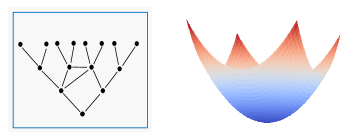
Figure 1. The (tree-like) graph $G$ in the left subfigure can be considered as a discrete approximation to the hyperbolic manifold $\mathcal{M}$ in the right subfigure; on the other hand, the hyperbolic manifold $\mathcal{M}$ can also be approximated as the graph $G$.

Tree-like structures refer to networks, systems, or data organizations that resemble a tree in their architecture, with nodes branching out from the root into multiple levels. They are widely observed in various real-world domains (Adcock et al., 2013; Abu-Ata and Dragan, 2016; Narayan and Saniee, 2011; Shavitt and Tankel, 2008; Zhou et al., 2022a; Liu et al., 2022c), such as recommendation systems, financial networks, and social networks.

Recently, the utilization of hyperbolic space for modeling tree-like structures has garnered substantial attention  (Nickel and Kiela, 2017, 2018; Chami et al., 2019; Liu et al., 2019; Zhang et al., 2021a; Ganea et al., 2018; Shimizu et al., 2020; Yang et al., 2022b; Peng et al., 2021). Compared with the zero curvature Euclidean space, one key property of negative curvature hyperbolic space is that it expand exponentially, making it can be considered as a continuous tree and vice versa (as shown in Figure 1). In other words, hyperbolic space allows for the efficient representation of a tree-like structure, as it enables nodes to be spread apart as they move away from the root, preventing crowding and overlapping of nodes as is commonly observed in Euclidean space. Additionally, hyperbolic space allows for exponential growth in the number of nodes in a given area, which is well-suited for modeling the exponential growth of trees.

However, the real-world dataset often deviates from a pure tree configuration and manifests in a labyrinthine complexity, posing large challenges for tree-likeness modeling within hyperbolic space  (Zhu et al., 2020; Wang et al., 2021b). For instance, biological taxonomies, which depict the hierarchical relationships between different species from a global view, often exhibit both extensive local flat regions where multiple species are closely related and local circular regions where species connections are less defined. The local structure of a tree-like graph exhibits a heterogeneous blend of tree-like, flat, and circular patterns, resulting in difficulties in uniformly embedding the data into a homogeneous embedding space and thereby engendering structural biases and distortions.

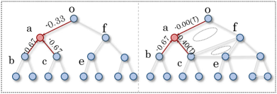
Figure 2. Illustration of two tree-like graphs: $T_{1}$ (left) is pure and $T_{2}$ (right) has a local heterogeneous structure. The arrows indicate the aggregation flow and the values on the edges represent the edge curvature, denoted as $\kappa^{1}$ for $T_{1}$ and $\kappa^{2}$ for $T_{2}$. By incorporating curvature $\kappa$ into the neighboring aggregation, the detection of local structures is improved. This is achieved by assigning asymmetric weights ($\kappa_{a,o}^{1}$ vs $\kappa_{a,b}^{1}$) to nodes at different levels and results in larger values for nodes in a circular shape ($\kappa_{a,o}^{1}$ vs $\kappa_{a,o}^{2}$ and $\kappa_{a,c}^{1}$ vs $\kappa_{a,c}^{2}$).

To mitigate the limitations, this study seeks to examine the intersection between the discrete structure of the data and the continuous learning space. The aim is to encode the information inherent in the network topology in a manner that is both effective and imbued with structural inductive bias, thereby enhancing the performance of downstream tasks. From a geometric perspective, the quality of the embedding in geometric learning depends on the compatibility between the intrinsic graph structure and the embedding space (Gu et al., 2019). In light of this principle, we employs the concept of curvature to guide tree-likeness modeling in hyperbolic space. As shown in Figure 2, the incorporation of curvature information offers a more comprehensive grasp of the local shape characteristics, facilitating the representation of the shape and contours of diverse regions within the learning space.

In Riemannian geometry, curvature measures the deviation of a geometric object from being flat, originally defined on continuous smooth manifolds (Lee, 2018). Smooth manifolds with positive, zero, or negative curvature are spherical, Euclidean, and hyperbolic spaces, respectively. This concept has been extended to discrete objects such as graphs, where curvature describes the deviation of a local pair of neighborhoods from a ”flat” case.

Graph curvature, analogous to curvature in the realm of continuous geometry, consists of Gaussian curvature, Ricci curvature, and mean curvature. These components have unique roles: Gaussian curvature quantifies the local curvature at vertices, Ricci curvature allocates curvature to the edges, and mean curvature provides an overall metric for the entire graph. In this work, we focus on Ricci curvature for graph convolution and edge-based filtering. Several definitions have been proposed about Ricci curvature, including Ollivier Ricci curvature (Ollivier, 2009), Forman Ricci curvature (Forman, 2003), Balanced Forman curvature (Topping et al., 2021). Ricci curvature controls the overlap between two distance balls by considering the radii of the balls and the distance between their centers (Jost and Liu, 2014). Furthermore, the lower bound of Ricci curvature can reveal valuable global geometric and topological information (Ambrose et al., 1957). It is also an effective indicator of tree-like, flat, and cyclic areas, making it well-suited for integration into hyperbolic space to capture asymmetries, biases, and hierarchies.

Overall, we put forward a novel framework: curvature-aware hyperbolic graph convolutional neural network ($\kappa$HGCN) for effectively modeling tree-like datasets with complex structures. Specifically, $\kappa$HGCN leverages the discrete Ricci curvature to guide message passing and dynamically adapts the global continuous hyperbolic curvature. Through empirical evaluations on diverse datasets and tasks, we confirm the superiority of the $\kappa$HGCN, as it consistently outperforms existing baselines by substantial margins. The major contributions of this work are summarized as follows:

• We design a novel hyperbolic geometric learning framework that encapsulates the graph Ricci curvature into the continuous embedding space, producing less distortion, powerful expressiveness, and topology-aware embeddings;

• We present a new message technique for hyperbolic graph embedding, and we further prove that it produces a smaller (larger) embedding distance when larger (smaller) curvature is involved, which well handles the inconsistency between the local structure and global curvature of embedding space;

• Extensive experiments demonstrate that the proposed model $\kappa$HGCN achieves significant improvements over various baselines on link prediction and node classification tasks.

2. Related Work

For tree-likeness modeling, we mainly review the latest research techniques including graph neural networks and hyperbolic geometry. In addition to this, we also review the recent advancements in curvature and curvature-based learning.

2.1. Graph Neural Networks

Tree-structured data can often be represented as graphs. In recent years, graph neural networks (GNNs) have gained significant attention within the graph learning community. The main concept behind GNNs is a message-passing mechanism that aggregates information from neighboring nodes. GNNs have demonstrated remarkable performance in various tasks, including node classification, link prediction, graph classifications, and graph reconstruction (Kipf and Welling, 2017; Hamilton et al., 2017a; Veličković et al., 2018; Gasteiger et al., 2018; Ma et al., 2019; Morris et al., 2019; Zhang et al., 2022b; Zhang and Chen, 2018; Zhang et al., 2022a; Yang et al., 2020; Song et al., 2022, 2021a; Li et al., 2022; Zhang et al., 2022c; Liu et al., 2022a; Fu et al., 2020). They have also found wide applications in recommender systems, anomaly detection, social networks analysis, and more (Chen et al., 2022b, 2023a, a, c, 2023b; Dou et al., 2020; Ma et al., 2021; Kipf and Welling, 2017; Song et al., 2022; Song and King, 2022; Song et al., 2021b; Yang et al., 2022d). The majority of GNNs learn graphs in Euclidean space due to their computational advantages and intuitiveness. However, Euclidean models are limited in their ability to represent complex patterns in graph (Bouchard et al., 2015).

2.2. Hyperbolic Geometry

Hyperbolic representation learning has recently garnered considerable attention (Zhou et al., 2022b; Choudhary et al., 2022). Hyperbolic geometry has been recognized as a continuous tree (Krioukov et al., 2009), exhibiting properties such as low distortion and small generalization errors when modeling tree-like structured data (Sarkar, 2011; Suzuki et al., 2021a, b). Its applications span various domains (Yang et al., 2022b; Mettes et al., 2023; Peng et al., 2021), including computer vision (Khrulkov et al., 2020; Atigh et al., 2022; Hsu et al., 2021), natural language processing (Nickel and Kiela, 2017, 2018; Sala et al., 2018; Montella et al., 2021; Kolyvakis et al., 2019; Bai et al., 2021; Chami et al., 2020), recommender systems (Vinh Tran et al., 2020; Yang et al., 2022c; Sun et al., 2021; Wang et al., 2021a; Yang et al., 2022a; Chen et al., 2022c), graph learning (Gulcehre et al., 2018; Zhang et al., 2021a; Chami et al., 2019; Liu et al., 2019, 2022b; Yang et al., 2021; Bai et al., 2023) and more (Xiong et al., 2022a). In the graph learning domain, recent works (Liu et al., 2019; Chami et al., 2019; Lou et al., 2020; Zhang et al., 2021b, a; Yang et al., 2022d, 2021; Liu et al., 2022b) have generalized graph neural networks to hyperbolic space and demonstrated impressive performance, particularly on tree-like data. Some studies (Peng et al., 2020; Wang et al., 2021b; Zhu et al., 2020; Sun et al., 2022) propose learning graph in different embedding spaces or product spaces. Furthermore, researchers have also explored the use of ultrahyperbolic geometry for graph learning (Xiong et al., 2022b, 2021; Law and Stam, 2020; Law, 2021). However, many existing methods fail to consider the local heterogeneous structure of graphs, resulting in significant distortion and low-quality embeddings.

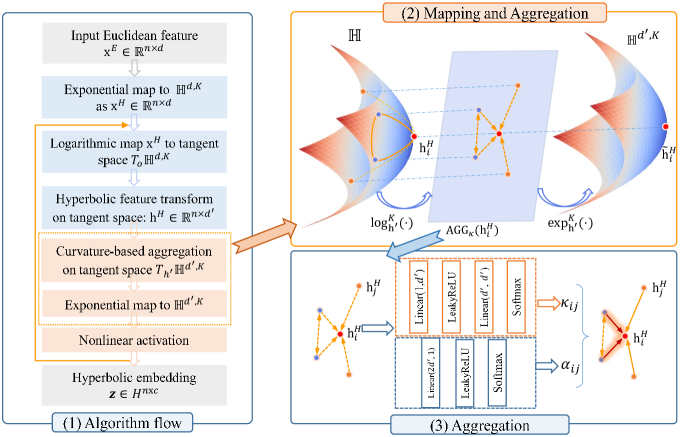
Figure 3. Schematic of $\kappa$HGCN. (1) The simplified algorithm flow of our method: consists of hyperbolic projection, feature transform, and aggregation. After that, a readout layer is applied to the embeddings for either a node classification or link prediction task. (2) The visualization of neighborhood aggregation procedure: first project information to hyperbolic space for transformation, then map messages to the tangent space, perform the aggregation in the tangent space with the guide of discrete curvature (and attention), and then map back to the hyperbolic space. (3) The details of Ricci Curvature-aware aggregation and its combination with feature-based attention.

2.3. Graph Curvature

Graph curvature, resembling curvature in continuous geometry, includes Gaussian curvature, Ricci curvature, and average curvature. Each of these elements serves a distinct purpose: Gaussian curvature measures local curvature at vertices, Ricci curvature assigns curvature to edges, and average curvature offers a global measure for the entire graph. Applications of graph curvatures span various domains in network alignment, congestion and vulnerability detection, community detection, and robustness analysis (Ni et al., 2018, 2015; Jonckheere et al., 2011). The recent work of curvature graph neural network (CurvGN) (Ye et al., 2019) introduced the notion of Ricci curvature into the field of graph learning. The study in (Topping et al., 2021) showed that edges with negative curvature can contribute to the over-squashing problem in graph embeddings. Coinciding with the announcement of the accepted papers for WWW 2023, we noted a parallel work by Fu et al. (Fu et al., 2023) that introduces the idea of class-aware Ricci curvature for addressing hierarchy-imbalance in node classification, while in our work, we aim to explore the integration of more generalized ricci curvature with hyperbolic graph convolution and curvature-based filtering mechanism to enhance the performance of HGCN for a more range of tasks, including node classification and link prediction.

3. Background

In this part, we first briefly review the necessary definitions of differential geometry, primarily concentrating on hyperbolic geometry. A thorough and in-depth explanation can be found in (Lee, 2018). We also give a short introduction about Ollivier Ricci curvature (ORC), which is a generalized Ricci curvature tailored for discrete objects (e.g., graphs) . The readers may refer to (Ollivier, 2009) for more details.

3.1. Riemannian Geometry

Manifold and Tangent Space. Riemannian geometry, a subfield of differential geometry, denoted as $\mathcal{M}$ with a Riemannian metric $g$. An $n$-dimensional manifold $(\mathcal{M},g)$ represents a smooth and real space, essentially an extension of a 2-D surface to higher dimensions, that can be locally approximated by $\mathbb{R}^{n}$. For any point $\mathbf{x}$ on $\mathcal{M}$, we define a tangent space $\mathcal{T}_{\mathbf{x}}\mathcal{M}$, acting as the first-order approximation of $\mathcal{M}$ in the vicinity of $\mathbf{x}$. This tangent space is an $n$-dimensional vector space that is isomorphic to $\mathbb{R}^{n}$. The metric $g$ on the Riemannian manifold designates a smoothly changing positive definite inner product $<\cdot,\cdot>:\mathcal{T}_{\mathbf{x}}\mathcal{M}\times\mathcal{T}_{\mathbf{x}}\mathcal{M}\to\mathbb{R}$ on this tangent space, thereby facilitating the definition of numerous geometric attributes, such as geodesic distances, angles, and curvature.

Geodesics and Induced Distance Function. For a curve $\gamma:[\alpha,\beta]\to\mathcal{M}$, the shortest length of $\gamma$, i.e., geodesics, is defined as $L(\gamma)=\int_{\alpha}^{\beta}\|\gamma^{\prime}(t)\|_{g}dt$. Then the distance of $\mathbf{u},\mathbf{v}\in\mathcal{M}$, $d^{\mathcal{M}}(\mathbf{u},\mathbf{v})=\inf L(\gamma)$ where $\gamma$ is a curve that $\gamma(a)=\mathbf{u},\gamma(b)=\mathbf{v}$.

Maps and Parallel Transport. The maps define the relationship between the hyperbolic space and the corresponding tangent space. Given a point $\mathbf{x}\in\mathcal{M}$ and a vector $\mathbf{v}\in\mathcal{T}_{\mathbf{x}}\mathcal{M}$, a unique geodesic $\gamma:[0,1]\to\mathcal{M}$ exists, satisfying $\gamma(0)=\mathbf{x},\gamma^{\prime}(0)=\mathbf{v}$. The exponential map, symbolized as $\exp_{\mathbf{x}}:\mathcal{T}_{\mathbf{x}}\mathcal{M}\to\mathcal{M}$, is defined such that $\exp_{\mathbf{x}}(\mathbf{v})=\gamma(1)$. Conversely, the logarithmic map, denoted as $\log_{\mathbf{x}}$, acts as the inverse of $\exp_{\mathbf{x}}$. Furthermore, the parallel transport $PT_{\mathbf{x}\rightarrow\mathbf{y}}:\mathcal{T}\mathbf{x}\mathcal{M}\to\mathcal{T}\mathbf{y}\mathcal{M}$ achieves the transportation from point $\mathbf{x}$ to point $\mathbf{y}$, while ensuring the preservation of the metric tensors.

Hyperbolic Models. Hyperbolic geometry describes a curved space with negative curvature. There are several mathematically equivalent ways to model hyperbolic geometry that emphasize different properties, but our methods apply to hyperbolic geometry in general and are not limited to any particular model. Formulas for concepts such as distance, maps, and parallel transport are summarized in Appendix B.

3.2. Graph Curvature

Curvature is a fundamental concept in smooth spaces that has also generalized to discrete objects (e.g., graphs). There are several distinct notions of discrete Ricci curvature for graphs or networks, such as the Forman-Ricci curvature (Forman, 2003) and Ollivier-Ricci curvature (Ollivier, 2009). Here we mainly focus on ORC since it is more geometrical (Ollivier, 2009; Jost and Liu, 2014). Another reason is ORC builds a bridge between continuous geometry and discrete structures (Van der Hoorn et al., 2020; Ache and Warren, 2019).

Definition 3.0 (Ollivier-Ricci Curvature).

Let $G=(V,E)$ be a locally finite, connected, and simple graph (i.e., $G$ contains no multiple edges or self-loops), for any two distinct vertices $v_{1},v_{2}$, the ORC of $v_{1}$ and $v_{2}$ is defined as

(1) $$\kappa(v_{1},v_{2})=1-\frac{W(m_{v_{1}},m_{v_{2}})}{d(v_{1},v_{2})}\in(-2,1),$$

where $d(v_{1},v_{2})$ is the shortest path between $v_{1}$ and $v_{2}$ on graph $G$, $W(m_{v_{1}},m_{v_{2}})$ is the Wasserstein distance (see Definition 3.2) between two probability measures (see Definition 3.3) $m_{v_{1}}$ and $m_{v_{2}}$.

Definition 3.0 (Wasserstein Distance).

Let $m_{1},m_{2}$ be two probability measures on $V$. The Wasserstein distance $W(m_{1},m_{2})$ between $m_{1}$ and $m_{2}$ is given by

(2) $$W(m_{1},m_{2})=\inf_{\pi_{i,j}\in\Pi}\sum_{v_{i},v_{j}\in V}\pi_{i,j}(v_{i},v_{j})d(v_{i},v_{j}),$$

where $\pi_{i,j}:V\times V\to[0,1]$ is a transport plan, i.e., the probability measure of the amount of mass transferred from $v_{i}$ to $v_{j}$. Then to seek an optimal transference plan ($\pi$) that is to minimize the total cost of moving from $v_{i}$ to $v_{j}$ such that for every $v_{i},v_{j}$ in $V$ satisfying

(3) $$\sum_{v_{i}\in V}\pi_{i,j}(v_{i},v_{j})=m_{1};\sum_{v_{j}\in V}\pi_{i,j}(v_{i},v_{j})=m_{2}.$$

Definition 3.0 (Probability Measure).

Given $G=(V,E)$, for a vertex $v_{i}$ in $V$, denote $d_{v_{i}}$ the degree of $v_{i}$ and $N(v)$ the neighbors of $v$, for any $p\in[0,1]$, the probability measure $m_{v_{i}}$ on $V$ is defined as:

(4) $$m_{v_{i}}=\left\{\begin{array}[]{ll}p,&\text{ if }v=v_{i}\\ \frac{1-p}{d_{v}},&\text{ if }(v_{i})\in N(v).\\ 0,&\text{ otherwise }\end{array}\right.$$

Geometric Intuition

ORC seeks the most efficient transportation plan that preserves mass between two probability measures, which may be solved using linear programming. Intuitively, transporting messages between two nodes whose neighbors are highly overlapping, such as two nodes in the same cluster, is costless. On the other hand, if two nodes are situated in distinct groups or clusters, information flow between them is difficult.

4. Methodology

The proposed method, $\kappa$HGCN, combines discrete and continuous curvatures to improve tree-like modeling in hyperbolic space. Our approach emphasizes the strengthening of message passing in nodes with high local graph curvature and the weakening of message propagation in nodes with low local curvature. This curvature-guided approach enhances the formation of hierarchies and reduces the impact of structural incompatibility on the modeling process.

4.1. $\kappa$HGCN

Our approach, named $\kappa$HGCN, presents a novel curvature-aware hyperbolic graph network model, as depicted in Figure 3. Building upon the foundation of HGCN (Chami et al., 2019), we implement graph convolution operations via the tangential method (Chami et al., 2019; Liu et al., 2019) space. However, it is worth mentioning that $\kappa$HGCN is flexible and can be applied to non-tangential methods as well (Zhang et al., 2021b). Similar to other GNN and HGNN models, $\kappa$HGCN also comprises three fundamental modules: hyperbolic feature transformation, curvature-aware neighbor aggregation, and non-linear activation.

4.1.1. Hyperbolic Feature Transformation

Hyperbolic feature transformation is formulated as:

(5) $$\mathbf{h}_{i}^{\ell,\mathcal{H}}=\left(\mathbf{W}^{\ell}\otimes^{\kappa_{\ell-1}}\mathbf{x}_{i}^{\ell-1,\mathcal{H}}\right)\oplus^{\kappa_{\ell-1}}\mathbf{b}^{\ell},$$

where $\ell$ denotes the $\ell$-th layer, $\mathbf{W}$ is the trainable matrix and $\mathbf{b}$ is the bias. $\mathbf{W}\otimes^{\kappa}\mathbf{x}:=\exp_{\mathbf{o}}^{\kappa}(\mathbf{W}\log_{\mathbf{o}}^{\kappa}(\mathbf{x}))$ and $\mathbf{x}\oplus^{\kappa}\mathbf{b}:=\exp^{\kappa}_{\mathbf{x}}(PT_{\mathbf{o}\rightarrow\mathbf{x}}^{\kappa}(\mathbf{b}))$ are matrix-vector multiplication and bias translation operations in hyperbolic space, respectively. The superscript ^H denotes the hyperbolic feature.

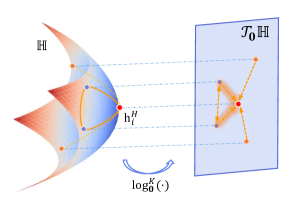
Figure 4. Illustration of the proposed Curvature-aware aggregation. Compared with the traditional aggregation scheme, the proposed method further makes the aggregation process aware of the local structure.

4.1.2. Curvature-Aware Neighbor Aggregation

Curvature-Aware Neighbor Aggregation, as shown in Figure 4, is built in the tangent space of the origin:

(6) $${\tilde{\mathbf{h}}_{i}^{\ell,\mathcal{H}}=\exp_{\mathbf{o}}^{\kappa_{l-1}}\left(\sum_{j\in\mathcal{N}_{i}}{\tilde{\kappa}_{i,j}\cdot\log_{\mathbf{o}}^{\kappa_{l-1}}(\mathbf{h}_{j}^{\ell,\mathcal{H}})}\right)}.$$

Here $\tilde{\kappa}_{i,j}$ denotes the curvature for capturing the local structure, computed by softmax operation within the neighbors $\mathcal{N}_{i}$ ($\mathcal{N}_{i}$ contains the node self):

(7) $$\tilde{\kappa}_{i,j}=\textrm{softmax}_{j\in\mathcal{N}(i)}\left(\textrm{MLP}(\kappa_{i,j})\right),$$

where $\kappa_{i,j}$ is the raw ORC value, and MLP (Multilayer Perceptron) is employed to make the curvature more adaptive to the overall negative curvature. This approach is referred to as Curv. When it comes to the case where the topology information and node features are inconsistent to a certain degree, e.g., the network is quite sparse or depends more on the node features, inspired by (Zhang et al., 2020), we propose a feature-attention enhanced aggregation (CurvAtt), which encodes node state into the curvature:

(8) $$\tilde{\kappa}^{\prime}_{i,j}=\frac{w_{\kappa}\tilde{\kappa}_{i,j}+w_{\alpha}\alpha_{i,j}}{w_{\kappa}+w_{\alpha}},$$

where $\alpha_{i,j}$ is hyperbolic feature attention, $w_{\kappa}$ and $w_{\alpha}$ are the trainable parameters that adjust structure information and feature correlation with the initial value $1.0$. The hyperbolic feature attention $\alpha_{i,j}$ is defined as:

(9) $${\alpha}_{i,j}=\mathrm{softmax}_{j\in\mathcal{N}_{i}}\left(\textrm{MLP}(\log_{\mathbf{o}}^{\kappa}(\mathbf{h}_{i}^{\mathcal{H}})\|\log_{\mathbf{o}}^{\kappa}(\mathbf{h}_{j}^{\mathcal{H}}))\right).$$

4.1.3. Hyperbolic Non-linear Activation

After that, we apply a nonlinear activation:

(10) $$\mathbf{x}_{i}^{\ell,\mathcal{H}}=\sigma^{{\kappa_{\ell-1},\kappa_{\ell}}}(\tilde{\mathbf{h}}^{\ell,\mathcal{H}})=\exp_{\mathbf{o}}^{\kappa_{\ell}}\left(\sigma(\log_{\mathbf{o}}^{\kappa_{\ell-1}}(\tilde{\mathbf{h}}^{\ell,\mathcal{H}}))\right).$$

Geometric Intuition

The real-world tree-like graphs with heterogeneous local structures are inevitably distorted if we directly embed them into a homogeneous manifold. For instance, the embedding of quasi-cycle graphs such as $n\times n$ square lattices (zero curvature) and $n$-node cycles (positive curvature) incur at least a multiplicative distortion of $O(n/\log n)$ in hyperbolic space (Verbeek and Suri, 2014). Graph Ricci curvature is able to mitigate this distortion. The geometric intuition is that the more positive the curvature is, the more two distance balls centered at nearby points overlap, and therefore, the cheaper it is to transport the mass from one to the other. Theoretical results show that with the increasing number of triangles involved in the linked pair $(i,j)$, the lower bound of curvature will be increased (Jost and Liu, 2014), as stated in Theorem 4.1. It is easy to understand because when the two vertices share many triangles, then the transportation distance should be smaller, and the curvature, therefore, is correspondingly larger.

Theorem 4.1 (Lower bound of ORC (Jost and Liu, 2014)).

On a locally finite graph, for any pair of neighboring vertices i, j, let $\#(i,j):=$ number of triangles which include $i,j$ as vertices for $i\sim j$. Then, we have the inequality, saying that

(11) $$\kappa_{i,j}\geq -\left(1-\frac{1}{d_{i}}-\frac{1}{d_{j}}-\frac{\#(i,j)}{d_{i}\wedge d_{j}}\right)_{+}$$

$$-\left(1-\frac{1}{d_{i}}-\frac{1}{d_{j}}-\frac{\#(i,j)}{d_{i}\vee d_{j}}\right)_{+}+\frac{\#(i,j)}{d_{i}\vee d_{j}},$$

where $s_{+}:=\max(s,0),s\vee t:=\max(s,t),\quad and\quad s\wedge t:=\min(s,t).$

In this study, we make a theoretical analysis in Theorem 4.2, which further demonstrates the relations of ORC and embedding distance, i.e., when a large curvature is involved within the linked node, the closer of their embedding distance, which thus mitigates the distortion.

Theorem 4.2 (Embedding Distance w.r.t ORC).

Let $(i,j)\in E$ be the linked pair, $\mathbf{h}_{i},\mathbf{h}_{j}\in\mathbb{R}^{d}$ be the node state in the tangent space, $d_{i}$ be the degree of node $i$, and $D$ be the distance of node $i$ and node $j$ in the tangent space, that is

(12) $${D}=\|\mathbf{h}_{i}-\mathbf{h}_{j}\|,$$

where $\|\cdot\|$ is the Euclidean norm. Define a large ORC as $\tilde{\kappa}_{i,j}>\max\{1/d_{i},1/d_{j}\}$ and a small ORC as $\tilde{\kappa}_{i,j}<\min\{1/d_{i},1/d_{j}\}$. Then, when the large ORC is involved, their embedding distance will get smaller if using $\kappa$HGCN. On the contrary, when the small ORC is involved, their embedding distance will get larger.

Proof.

In the following, we use ${D}_{l}$ and ${D}_{s}$ to denote the distance when large and small curvature $\tilde{\kappa}$ are involved, respectively. The main idea is that when there is a large curvature involved, the node distance will be decreased compared with the original case (degree-based aggregation), that is ${D}_{l}<{D}$. At the same time, when there is a small curvature involved, the node distance will increase, that is ${D}_{s}>{D}$.

(1) When a large curvature (i.e., $\kappa_{i,j}>\max(1/d_{i},1/d_{j})$) is involved, more messages will be transferred, and we decompose the embedding, taking $\mathbf{h}_{i}$ as an example, into two components: one is from original $\mathbf{h}_{i}$ and another is the incremental parts from $\mathbf{h}_{j}$, then

(13) $${D}_{l} =\|(\mathbf{h}_{i}+\alpha_{i}\mathbf{h}_{j})-(\mathbf{h}_{j}+\alpha_{j}\mathbf{h}_{i})\|$$

$$=\|(\mathbf{h}_{i}-\alpha_{j}\mathbf{h}_{i})-(\mathbf{h}_{j}-\alpha_{i}\mathbf{h}_{j})\|,$$

where $\alpha_{i}$ ($\alpha_{j}$) is the difference between $\tilde{\kappa}_{i,j}$ and $1/d_{i}$ ( $1/d_{j}$), i.e., $\alpha_{i}=\tilde{\kappa}_{i,j}-1/d_{i}$, $\alpha_{j}=\tilde{\kappa}_{i,j}-1/d_{j}$. Since $\tilde{\kappa}_{i,j}>\max(1/d_{i},1/d_{j})$, $\alpha_{i}$ and $\alpha_{j}$ are both positive. Let $\alpha_{ij}=\alpha_{i}\approx\alpha_{j}$, then

(14) $${D}_{l} \approx\|(\mathbf{h}_{i}-\alpha_{ij}\mathbf{h}_{i})-(\mathbf{h}_{j}-\alpha_{ij}\mathbf{h}_{j})\|$$

$$=(1-\alpha_{ij})\|\mathbf{h}_{i}-\mathbf{h}_{j}\|$$

$$<{D}.$$

Then, we easily know that when large curvature is involved, the distance will be reduced and two nodes will be closer to each other. What’s more, the larger the curvature, the closer the nodes are.

(2) Similarly, when a small curvature ($\kappa_{i,j}<\min(1/d_{i},1/d_{j})$) is involved, fewer messages will be transferred, and we decompose the embedding, taking $\mathbf{h}_{i}$ as an example, into two components: one is from original $\mathbf{h}_{i}$ and another is the reduction parts of $\mathbf{h}_{j}$, that is

(15) $${D}_{s} =\|(\mathbf{h}_{i}-\beta_{i}\mathbf{h}_{j})-(\mathbf{h}_{j}-\beta_{j}\mathbf{h}_{i})\|$$

$$\approx(1+\beta_{ij})\|\mathbf{h}_{i}-\mathbf{h}_{j}\|$$

$$>{D},$$

where $\beta_{i}$ is the difference between $1/d_{i}$ and $\tilde{\kappa}_{i,j}$, i.e., $\beta_{i}=1/d_{i}-\tilde{\kappa}_{i,j}$, $\beta_{j}=1/d_{j}-\tilde{\kappa}_{i,j}$. Both $\beta_{i}$ and $\beta_{j}$ are positive in that $\kappa_{i,j}<\min(1/d_{i},1/d_{j})$. Let $\beta_{ij}=\beta_{i}\approx\beta_{j}$, then, we easily know that when small curvature is involved, the node pair will become more distant in the embedding space. What’s more, the smaller the curvature, the more distant the nodes are. ∎

4.2. Curvature-based Homophily Constraint

In the degree-based learning paradigm, like GCN (Kipf and Welling, 2017), the influence of a node on another node decays exponentially as their graph distance increases as shown by (Huang and Zitnik, 2020). The analysis in (Huang and Zitnik, 2020) is limited degree-based aggregation and Euclidean space. The hyperbolic message passing learning paradigm of $\kappa$HGCN also shows a similar phenomenon, which causes too much influence loss in long-term propagation. Especially, if the paths consist of numerous connections to other nodes, the node influence is minimal. For clarity, we term the hyperbolic message passing learning paradigm in $\kappa$HGCN or original HGNNs (Liu et al., 2019; Chami et al., 2019; Zhang et al., 2021a) as HMP. The HMP is a local aggregation method, in which the influence of nodes decreases with increasing distance, as demonstrated in Theorem 4.3.

Theorem 4.3 (Decaying property of HMP).

Let $p$ be a path between node ${u}$ and node ${v}$, $d_{g}^{*}$ be the shortest distance between ${u}$ and ${v}$, let $C$ be a constant and $\mathbf{z}$ be the embedding on the tangent space. Consider the node influence $I_{{u},{v}}$ ($I_{u,v}=\|{\partial{\mathbf{z}_{u}}}{/\partial{\mathbf{z}_{v}}}\|$) from ${v}$ to ${u}$ using HMP, $I_{{u},{v}}\leq C\gamma^{d_{g}^{*}}(0<\gamma<=1)$. The condition for equality is $d_{g}^{*}=1$, and ${v}$ is the unique neighbors of node ${u}$, correspondingly $C=1,\gamma=1$.

Proof.

Recall the aggregation rule in Equations (6) and (7) (similar to that in origin HGNNs), we focus on the aggregation in the tangent space and ignore the previous logarithmic map and the later exponential map since they are applied before and after the whole aggregation process, respectively. Then for any node ${u}$ and ${v}$, the update rule in the tangent space can be formulated as:

(16) $$\mathbf{z}_{u}=\sum_{j\in\mathcal{N}(u)}{\tilde{\kappa}_{u,j}\mathbf{z}_{j}}=\frac{1}{K_{uu}}\sum_{j\in\mathcal{N}(i)}\exp(\tilde{\kappa}_{u,j})\mathbf{z}_{j},$$

where $K_{uu}={\sum_{j\in\mathcal{N}(u)}{\exp(\tilde{\kappa}_{u,j})}}.$ By an expansion of node in the neighbor $\mathcal{N}(j)$, we have:

(17) $$\mathbf{z}_{u}=\frac{1}{K_{uu}}\sum_{j\in\mathcal{N}(u)}\exp(\tilde{\kappa}_{u,j})*\frac{1}{K_{jj}}\sum_{k\in\mathcal{N}(j)}\exp(\tilde{\kappa}_{j,k}){\mathbf{z}}_{k}.$$

We completely expand it:

(18) $$\mathbf{z}_{u}= \frac{1}{K_{uu}}\sum_{j\in\mathcal{N}(u)}\exp(\tilde{\kappa}_{i,j})*\cdots*\frac{1}{K_{oo}}\sum_{p\in\mathcal{N}(o)}\exp(\tilde{\kappa}_{o,p}){\mathbf{z}}_{p}.$$

Node influences $I_{u,v}$ of $v$ on $u$ in the message passing output is $I_{u,v}=\|{\partial{\mathbf{z}_{u}}}{/\partial{\mathbf{z}_{v}}}\|$, where the norm is any subordinate norm and the node influence measures how a change in $v$ passes to a change in $u$. By equation (18), the node influence can be computed as:

(19) $$I_{u,v}=\|\frac{\partial\mathbf{z}_{u}}{\partial\mathbf{z}_{v}}\|$$

$$=\|\frac{\partial}{\partial\mathbf{z}_{v}}(\frac{1}{K_{uu}}\sum_{j\in\mathcal{N}(u)}\exp(\tilde{\kappa}_{i,j})*\cdots*{\frac{1}{K_{oo}}}\sum_{p\in\mathcal{N}(o)}\exp(\tilde{\kappa}_{o,p})\mathbf{z}_{p})\|.$$

The partial derivative of the nodes in Equation  (19) is zero if they are not on the path between node $u$ and $v$, and then the feature influence can be decomposed into the sum influence of all related paths. Suppose there are $n$ paths between $u$ and $v$, then

(20) $$I_{u,v}=\left\|\frac{\partial}{\partial\mathbf{z}_{v}}\left(I_{p_{1}}+\cdots+I_{p_{i}}\cdots+I_{p_{n}}\right)\right\|,$$

where

$$I_{p_{i}}=\underbrace{\frac{1}{K_{uu}}\exp(\tilde{\kappa}_{u,p_{j}^{i}})\cdots\frac{1}{K_{p_{n_{i}}^{i}p_{n_{i}}^{i}}}\exp(\tilde{\kappa}_{p_{n_{i}}^{i},v})}_{S(I_{p_{i}})}\mathbf{z}_{v}.$$

Note that, in Equation (20), the scalar term $S(I_{p_{i}})$ ranges from $(0,1]$ and all $I_{p_{i}}(1\leq i\leq n)$ have the term $m_{v}$, thus we separate $S(I_{p_{i}})$ and the rest derivative term and then uses the absolute homogeneous property, i.e., $\|\alpha M\|=|\alpha|\|M\|$

(21) $$I_{u,v} =\left|S(I_{p_{1}})+\cdots+S(I_{p_{i}})\cdots+S(I_{p_{n}})\right|\|\frac{\partial z_{v}}{\partial z_{v}}\|$$

$$=\left|S(I_{p_{1}})+\cdots+S(I_{p_{i}})\cdots+S(I_{p_{n}})\right|$$

$$\leq|n*\max(S(I_{p_{i}}))|$$

$$=|n*\gamma^{n^{i}}|$$

$$\leq|n*\gamma^{d_{g}^{*}}|$$

$$=C\gamma^{d_{g}^{*}},$$

where $d_{g}$ is the shortest path between $u$ and $v$, $d^{*}\leq n^{i}$ and $0<\gamma\leq 1$, thus the second inequality holds on in Equation (21). For more generality, we use constant $C$ to denote the $n$. The condition for equality is if and only if $d_{g}^{*}=1$ and the $v$ is the unique neighbor of node $u$, i.e., $\gamma=1$ and $C=1$. ∎

Table 1. Comparisons of the abilities of models in terms of global tree-likeness modeling (Global), local heterogeneous structure learning (Local), and neighbor interaction (Neighbor) are indicated by $\checkmark$ for the presence of the ability and $\times$ for its absence.

Model Type	Models	Global	Local	Neighbor
Shallow models	EUC	$\times$	$\times$	$\times$
	HYP	$\checkmark$	$\times$	$\times$
Euclidean GNN models	GCN	$\times$	$\times$	$\checkmark$
	GAT	$\times$	$\times$	$\checkmark$
	SAGE	$\times$	$\times$	$\checkmark$
	SGC	$\times$	$\times$	$\checkmark$
Curvature GNN models	CurvGN	$\times$	$\checkmark$	$\checkmark$
	$\kappa$GCN	$\checkmark$	$\times$	$\checkmark$
Hyperbolic GNN models	HGCN	$\checkmark$	$\times$	$\checkmark$
	LGCN	$\checkmark$	$\times$	$\checkmark$
Curvature-aware HGNN model	$\kappa$HGCN	$\checkmark$	$\checkmark$	$\checkmark$

Theorem 4.3 shows that the node influence using HMP exponentially decays as the shortest graph distance $d_{g}^{*}$ between two nodes increases. In other words, distant nodes in dense areas will have less interaction, even if they are in a dense connected area. To alleviate the phenomenon, we propose a Curvature-based Homophily Constraint ($\kappa$HC) to enhance the connection within linked pairs. The basic idea is to push the embeddings of linked nodes closer if their ORC value is larger than a threshold. In this way, we can enforce disjoint node pairs in dense areas or clusters to have more influence on each other through their mutual neighbors, which is given by:

(22) $$\mathcal{L}_{\kappa hc_{+}}=-\frac{1}{|E_{\kappa}|}\sum_{(i,j)\in E_{\kappa}}\mathrm{log}~{}p(\mathbf{x}_{i}^{\ell,\mathcal{H}},\mathbf{x}_{j}^{\ell,\mathcal{H}}),$$

where $E_{\kappa}$ is the filtered edge set based on ORC threshold $\tau$; $p(\cdot)$ is the Fermi-Dirac function, indicating the probability of two hyperbolic nodes $(u,v)$ link or not, which is given by:

(23) $$p(\mathbf{x}_{u},\mathbf{x}_{v})=\left[\exp{(d_{\mathcal{H}}^{2}(\mathbf{x}_{u},\mathbf{x}_{v})-r)/t}+1\right]^{-1},$$

and $d_{\mathcal{H}}(\mathbf{x}_{u},\mathbf{x}_{v})$ is the hyperbolic distance from $u$ to ${v}$, $r$ and $t$ is hyper parameters and we set it as previous work (Chami et al., 2019). We also sample the same number of negative link pairs that they have no connections or the curvature is very small based on the results in (Topping et al., 2021). Totally,

(24) $$\mathcal{L}_{\kappa hc}=\mathcal{L}_{\kappa hc_{+}}+\mathcal{L}_{\kappa hc_{-}}.$$

Geometric Intuition

HMP helps build the connection between the graph topology and the embedding space, adjust the curvature of the hyperbolic geometry, and guide the information flow. It also shortens the distance of two linked nodes in an area with many triangles, helping mitigate the distortion caused by hyperbolic space. Nonetheless, HMP is local inherently, and the proposed $\kappa$HC further enhances the interactions of unconnected nodes, which is non-local.

4.3. $\kappa$HGCN Architecture

Given the Euclidean feature $\mathbf{x}^{E}$, we first project it into the hyperbolic manifold by the exponential map. $\kappa$HGCN architecture takes layers of HMP as the encoder. Following the literature, the Fermi-Dirac function is used as a decoder in the link prediction task. For the node classification task, the final hyperbolic vector is mapped back to tangent space and decoded with MLP, which is the same with work (Chami et al., 2019).

Table 2. Statistics of the datasets

Dataset	Nodes	Edges	Classes	Node features	Hyperbolicity$\delta$
Disease (NC)	1044	1043	2	1000	0
Disease (LP)	2665	2664	2	1000	0
Airport	3188	18631	4	4	1
PubMed	19717	88651	3	500	3.5
Cora	2708	5429	7	1433	11

5. Experiments

Table 3. Profiling evaluation on node classification. F1-score with standard deviation for Disease and Airport; accuracy for others (the higher, the better).

Dataset	Disease	Airport	PubMed	Cora
Hyperbolocity ($\delta$)	0	1	3.5	11
EUC	$32.5\pm 1.1$	$60.9\pm 3.4$	$48.2\pm 0.7$	$23.8\pm 0.7$
HYP (Nickel and Kiela, 2017)	$45.5\pm 3.3$	$70.2\pm 0.1$	$68.5\pm 0.3$	$22.0\pm 1.5$
GCN (Kipf and Welling, 2017)	$69.7\pm 0.4$	$81.4\pm 0.6$	$78.1\pm 0.2$	$81.3\pm 0.3$
GAT (Veličković et al., 2018)	$70.4\pm 0.4$	$81.5\pm 0.3$	$79.0\pm 0.3$	${83.0}\pm 0.7$
SAGE (Hamilton et al., 2017b)	$69.1\pm 0.6$	$82.1\pm 0.5$	$77.4\pm 2.2$	$77.9\pm 2.4$
SGC (Wu et al., 2019)	$69.5\pm 0.2$	$80.6\pm 0.1$	$78.9\pm 0.0$	$81.0\pm 0.1$
CurvGN (Ye et al., 2019)	${89.8}\pm 2.9$	$84.7\pm 1.5$	$78.3\pm 0.3$	$82.0\pm 0.9$
$\kappa$GCN (Bachmann et al., 2020)	$82.1\pm 1.1$	$84.4\pm 0.4$	$78.3\pm 0.6$	$80.8\pm 0.6$
HGCN (Chami et al., 2019)	$74.5\pm 0.9$	${90.6}\pm 0.2$	${80.3}\pm 0.3$	$79.9\pm 0.2$
LGCN (Zhang et al., 2021b)	$84.4\pm 1.0$	$90.9\pm 1.0$	$78.8\pm 0.5$	$\textbf{83.3}\pm 0.5$
$\kappa$HGCN (Ours)	$\textbf{92.3}\pm 1.4$	$\textbf{92.8}\pm 0.4$	$\textbf{82.1}\pm 0.5$	${82.5}\pm 0.6$
$\Delta_{E}(\%)$	$+31.1$	$+13.0$	$+3.9$	$-0.6$
$\Delta_{\kappa}(\%)$	$+2.8$	$+9.6$	$+4.9$	$+0.6$
$\Delta_{H}(\%)$	$+2.2$	$+3.6$	$+5.0$	$+5.4$

Table 4. Profiling evaluation on link prediction. AUC scores with standard deviation are reported (the higher, the better). The best is bold.

Dataset	Disease	Airport	PubMed	Cora
Hyperbolicity($\delta$)	0	1	3.5	11
EUC	$60.9\pm 3.4$	$92.0\pm 0.0$	$83.3\pm 0.1$	$82.5\pm 0.3$
HYP (Nickel and Kiela, 2017)	$70.2\pm 0.1$	$94.5\pm 0.0$	$87.5\pm 0.1$	$87.6\pm 0.2$
GCN (Kipf and Welling, 2017)	$64.7\pm 0.5$	$89.3\pm 0.4$	$91.1\pm 0.5$	$90.4\pm 0.2$
GAT (Veličković et al., 2018)	$69.8\pm 0.3$	$90.5\pm 0.3$	$91.2\pm 0.1$	$93.7\pm 0.1$
SAGE (Hamilton et al., 2017a)	$65.9\pm 0.3$	$90.4\pm 0.5$	$86.2\pm 1.0$	$85.5\pm 0.6$
SGC (Wu et al., 2019)	$65.1\pm 0.2$	$89.8\pm 0.3$	$94.1\pm 0.0$	$91.5\pm 0.1$
CurvGN (Ye et al., 2019)	$80.6\pm 0.8$	$89.5\pm 0.3$	$91.6\pm 0.4$	$72.5\pm 0.7$
$\kappa$GCN (Bachmann et al., 2020)	$92.0\pm 0.5$	$92.5\pm 0.5$	$94.9\pm 0.3$	$92.6\pm 0.4$
HGCN (Chami et al., 2019)	$90.8\pm 0.3$	$96.4\pm 0.1$	${96.3}\pm 0.0$	$92.9\pm 0.1$
LGCN (Zhang et al., 2021b)	${96.6}\pm 0.6$	${96.0}\pm 0.6$	${96.6}\pm 0.1$	${93.6}\pm 0.4$
$\kappa$HGCN (Ours)	$\textbf{96.7}\pm 0.1$	$\textbf{98.2}\pm 0.1$	$\textbf{96.7}\pm 0.1$	$\textbf{95.0}\pm 0.1$
$\Delta_{E}(\%)$	$+27.2$	$+8.5$	$+2.8$	$+1.4$
$\Delta_{\kappa}(\%)$	$+4.1$	$+6.2$	$+1.9$	$+2.6$
$\Delta_{H}(\%)$	$+0.6$	$+0.2$	$+1.3$	$+1.1$

5.1. Experimental Setup

Datasets. The evaluation of our work utilizes several datasets, including Disease, Airport, and three benchmark citation networks, namely PubMed and Cora. While Disease and Airport exhibit a more hierarchical structure, the citation networks are less so, making them suitable for demonstrating the generalization capability of our proposal. In Table 2, we provide the data statistics and hyperbolicity metric that measures the tree-likeness of each graph. For further details, please refer to Appendix A.

Baselines. We compare our proposed model with various baselines. (1) Shallow Euclidean and hyperbolic models, including Euclidean embeddings (EUC) and Poincaré embeddings (HYP) (Nickel and Kiela, 2017); (2) Euclidean GNN models, i.e., GCN (Kipf and Welling, 2017), GraphSAGE (SAGE) (Hamilton et al., 2017a), Graph Attention Networks (GAT) (Veličković et al., 2018), Simplified Graph Convolution, (SGC) (Wu et al., 2019); (3) Curvature GNN models, including Curvature Graph Network (CurvGN) (Ye et al., 2019) which applies the discrete curvature in Euclidean model and ProdGCN which deploys GNNs to products of constant curvature spaces, both of them are close to our work; Hyperbolic GNNs, including HGCN (Chami et al., 2019), HGNN (Liu et al., 2019), HGAT (Zhang et al., 2021a), LGCN (Zhang et al., 2021b). Table 1 presents the different features of the aforementioned models regarding their capabilities for perceiving both global tree-likeness modeling and local heterogeneous structure, as well as their interactional aptitude with regard to neighboring information.

Experimental Details Data split. We evaluate $\kappa$HGCN on both node classification and link prediction tasks. The data split is the same with the previous works (Chami et al., 2019). More specifically, in link prediction, we randomly split edges into 85%, 5%, 10% for training, validation, and test sets, respectively. For node classification, we split nodes into 70%, 15%, 15% for Airport, 30%, 10%, 60% for Disease, and we use 20 labeled train examples per class for Cora, and PubMed. Implementation details. We closely follow the parameter settings as HGCN (Chami et al., 2019), fix the number of embedding dimensions to 16 and then perform hyper-parameter search on a validation set over learning rate, weight decay, dropout, and the number of layers. We also adopt the early stopping strategies based on the validation set as (Chami et al., 2019). For baselines, we mainly refer to the reported results in the literature, and for the inconsistent cases (such as different embedding dimensions in H2H-GCN), we re-implement their official code in similar experimental settings. Evaluation metric. Following the literature, we report the F1-score for Disease and Airport datasets, and accuracy for the others in the node classification tasks. For the link predictions task, the Area Under Curve (AUC) is calculated.

5.2. Experimental Results

We report the results of 10 random experiments, including standard deviations in TABLE 4 and 4, where the $\Delta_{E},\Delta_{\kappa},\Delta_{H}$ is the improvement of the proposed model $\kappa$HGCN over the Euclidean GNNs, Curvature-related GNNs and Hyperbolic GNNs, respectively.

Node Classification

The experimental results of node classification are summarized in TABLE 4, where a lower hyperbolicity value corresponds to a more tree-like structure. The key findings are: (1) Overall, the proposed model performs impressively, surpassing previous models on four out of five datasets. Specifically, hyperbolic models (e.g., HGCN, LGCN) perform substantially better on the more hyperbolic dataset (e.g., Disease) than on the less hyperbolic dataset; Euclidean models (e.g., GCN, GAT) find more success on the less hyperbolic datasets (e.g., Cora) than on the more hyperbolic dataset; whereas our model performs better on both datasets, which is consistent with our motivation, namely, that the graph can be better learned under the guidance of curvature. In addition, from the improvements of $\Delta_{\kappa}$, we discovered that CurvGN with discrete curvature and $\kappa$GCN with continuous curvature both perform worse than our method which validates the power of hyperbolic geometry and the curvature-aware learning. (3) When it comes to Cora, both hyperbolic models and the proposed $\kappa$HGCN fail to outperform Euclidean GAT (Veličković et al., 2018), indicating Euclidean geometry is more suitable for modeling data with scarcely hierarchical structures. Nevertheless, it is noted that $\kappa$HGCN still outperforms well-known Euclidean GCN models, e.g., GCN (Kipf and Welling, 2017), SGC (Wu et al., 2019), SAGE (Hamilton et al., 2017a). It is observed that the proposed method $\kappa$HGCN also helps to narrow down the gap between hyperbolic models and Euclidean GAT.

Link Prediction

The experimental results of link prediction tasks are summarized in TABLE 4. In the link prediction task, we further have the following observations: (1) Compared with Euclidean counterparts, Our proposed $\kappa$HGCN, and other hyperbolic models have achieved better performance. It is because hyperbolic space owns a larger embedding space, where the structural dependencies could be well preserved by the link prediction loss, providing more space or boundary for nodes to be well arranged; (2) In comparison with the advanced hyperbolic models, our model also obtains remarkable gains and refresh the records.

According to the above extensive experiments, we are safe to conclude that equipping ORC with hyperbolic geometry further improves its generalization ability, obtaining high-quality representations for both tree-like and non-tree-like structured data. This confirms our primary motivation that the curvature carries rich information which is beneficial for graph representation learning in the embedding manifold. Specifically, incorporating the structure information featured by ORC helps the models developed in a continuous manifold with negative curvature to perceive the role of each node, accelerating the learning procedure, and reducing the distortion for graph embedding of less hierarchical networks.

5.3. Effectiveness of Aggregations

Table 5. Performance of different aggregation methods: curvature (Curv) and feature-enhanced curvature (CurvAtt).

Dataset	NC		LP
	Curv	CurvAtt	Curv	CurvAtt
Disease	$91.8\pm 1.9$	$\textbf{92.3}\pm 1.4$	$95.7\pm 0.3$	$\textbf{95.8}\pm 0.1$
Airport	$92.4\pm 1.0$	$\textbf{92.8}\pm 0.8$	$98.0\pm 0.1$	$\textbf{98.2}\pm 0.1$
PubMed	$81.2\pm 0.1$	$\textbf{82.1}\pm 0.4$	$96.5\pm 0.1$	$\textbf{96.7}\pm 0.1$
Cora	$82.3\pm 0.6$	$\textbf{82.5}\pm 0.6$	$94.9\pm 0.3$	$\textbf{95.0}\pm 0.5$

In Section 4.1, we introduce two tangential aggregation strategies: the curvature-based approach (denoted as Curv) and the feature-augmented method (denoted as CurvAtt). The performance of these two aggregation strategies is evaluated and reported in Table 5. Our results show that the feature-augmented approach outperforms the curvature-based one in most cases, which can be attributed to the complex nature of real-world systems and the incongruities between node features and topology. The feature-augmented method offers a more flexible and adaptive way to synthesize information from various sources, thus resulting in improved performance.

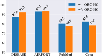
Figure 5. The performance of node classification by $\kappa$HGCN with $\kappa$HC and without $\kappa$HC.

5.4. Effectiveness of $\kappa$HC

Figure 5 displays the results of adding $\kappa$HC or not on $\kappa$HGCN. As it observed, the performance degenerates substantially on DISEASE when applying $\kappa$HC, while there are significant improvements on the three citation networks, i.e., PubMed, and Cora. This phenomenon can be understood as follows. Adding $\kappa$HC as in node classification will force linked nodes to obtain more similar representations. For the pure tree-like dataset, i.e., DISEASE (without any triangle and circle), these node pairs belong to different levels, and adding $\kappa$HC impairs the learning of asymmetric dependencies, which further affects the establishment of hierarchical awareness. When it comes to the citation networks instead, $\kappa$HC helps to reduce the distortion caused by hyperbolic geometry and thus boost the learning.

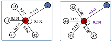
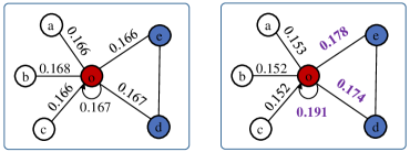
Figure 6. A tree-like area (upper row) and a triangle-contained area (lower row) with edge weights by HGCN (left column) and $\kappa$HGCN (right column).

5.5. Case Study of Ricci Curvature Weights

In this section, we demonstrate the effectiveness of our method through a case study. We extract a subtree centered on a randomly sampled node (node 10, in this case), from the Disease dataset, where node 2 is from a higher level and the remaining nodes (42, 43, 44, 45) belong to a lower level. The edges depict disease propagation paths. As shown in the upper sub-figures of Figure 6, we display the corresponding edge weights assigned by both $\kappa$HGCN and HGCN during the node classification task. The comparison between the two reveals that $\kappa$HGCN (upper right) effectively distinguishes node levels, as it assigns greater importance to the parent node (node 2) and equally emphasizes the child nodes from the same level, whereas HGCN (upper left) fails to make such distinctions. This substantiates the importance of ORC in facilitating hierarchical learning.

Furthermore, we illustrate a subgraph with triangles selected from the citation network, Cora, as depicted in the lower two sub-figures of Figure 6. This subgraph comprises nodes ${o,e,d}$ that form a triangle. We examine the edge weights around node $o$ and present the results in the lower two sub-figures of Figure 6. Observing these results, it is evident that $\kappa$HGCN (as shown in the lower right) effectively identifies the local triangle structure and assigns larger weights to promote inter-node message exchange. In contrast, HGCN (as depicted in the lower left) fails to grasp the intricate topology in this area. These observations further attest to the efficacy of our proposed method in uncovering local clusters and mitigating the distortions imposed by hyperbolic geometry.

6. Conclusion

For modeling tree-like structures, the hyperbolic space has demonstrated its ability to capture hierarchical relationships. However, approximating a discrete tree-like graph with a hyperbolic manifold can result in inevitable distortions, as real-world tree-like graphs are inherently complex. In this work, we integrate the intrinsic graph structure into the continuous hyperbolic embedding space via the discrete Ricci curvature. As expected, the graph curvature facilitates the node to perceive the role and the hierarchy it belongs to, helping accelerate the hierarchical formation as well as alleviate the distortion in local clusters or cliques. The superiority of the proposal is demonstrated by extensive experiments. Curvature is a geometric notion with appealing and descriptive properties for both network and continuous space. Via the interaction of curvatures, we can build proper connections for a graph and the embedding space to obtain high-quality representations, which is a promising direction to advance geometric learning. In the future, we will consider the use of Ricci flow, a more sophisticated geometric concept derived from Ricci curvature, to further enhance graph embedding and graph machine learning in tree-likeness modeling.

Appendix

Appendix A Datasets

In this section, we provide details about the datasets used in our study. The Disease dataset contains nodes that are labeled as infected or not infected with a disease, with features indicating their susceptibility to the disease. The disease-spreading network in this dataset displays a clear hierarchical structure, which makes it ideal for testing the effectiveness of hyperbolic embedding models. We use this dataset to validate our proposal. The Airport dataset consists of nodes representing airports, with edges indicating the existence of routes between two airports and labels reflecting the population of the respective country that the airport belongs to. In contrast, the PubMed and Cora datasets represent scientific papers as nodes, with edges indicating citations and labels corresponding to academic subfields. Additionally, the Disease and Airport datasets have imbalanced node labels, rendering accuracy an inadequate measure of model performance. Therefore, we use the F1 score as a more suitable measure for imbalanced datasets. Conversely, for the remaining datasets with balanced node classes, we use accuracy to evaluate the models. Furthermore, note that according to the official code of HGCN, the data statistics for Disease in node classification and link prediction differ slightly, and we list them separately in Table 2 for clarity.

Hyperbolicity $\delta$ is a metric that quantifies how closely a graph resembles a tree structure, with lower values of $\delta$ indicating greater tree-like characteristics. A $\delta$ value of 0 corresponds to a tree, while higher hyperbolicity values indicate a less tree-like structure. The relationship between hyperbolicity and tree-like characteristics has been established in various studies, including (Adcock et al., 2013; Narayan and Saniee, 2011; Jonckheere et al., 2011).

Table 6. Summary of operations in the Poincaré ball model and the Lorentz model ($\kappa<0$)

	Poincaré Ball Model	Lorentz Model (Hyperboloid Model)
Manifold	$\mathcal{B}_{\kappa}^{n}=\left\{\mathbf{x}\in\mathbb{R}^{n}:\langle\mathbf{x},\mathbf{x}\rangle_{2}<-\frac{1}{\kappa}\right\}$	$\mathcal{L}_{\kappa}^{n}=\left\{\mathbf{x}\in\mathbb{R}^{n+1}:\langle\mathbf{x},\mathbf{x}\rangle_{\mathcal{L}}=\frac{1}{\kappa}\right\}$
Metric	$g_{\mathbf{x}}^{\mathcal{B}_{\kappa}}=\left(\lambda_{\mathbf{x}}^{\kappa}\right)^{2}\mathbf{I}_{n}\text{ where }\lambda_{\mathbf{x}}^{\kappa}=\frac{2}{1+\kappa\|\mathbf{x}\|_{2}^{2}}$	$g_{\mathbf{x}}^{\mathcal{L}_{\kappa}}=\eta,\text{ where }\eta\text{ is }I\text{ except }\eta_{0,0}=-1$
Distance	$d_{\mathcal{B}}^{\kappa}(\mathbf{x},\mathbf{y})=\frac{1}{\sqrt{|\kappa|}}\cosh^{-1}\left(1-\frac{2\kappa\|\mathbf{x}-\mathbf{y}\|_{2}^{2}}{\left(1+\kappa\|\mathbf{x}\|_{2}^{2}\right)\left(1+\kappa\|\mathbf{y}\|_{2}^{2}\right)}\right)$	$d_{\mathcal{L}}^{\kappa}(\mathbf{x},\mathbf{y})=\frac{1}{\sqrt{|\kappa|}}\cosh^{-1}\left(\kappa\langle\mathbf{x},\mathbf{y}\rangle_{\mathcal{L}}\right)$
Logarithmic Map	$\log_{\mathbf{x}}^{\kappa}(\mathbf{y})=\frac{2}{\sqrt{|\kappa|\lambda^{\kappa}}}\tanh^{-1}\left(\sqrt{|\kappa|}\left\|-\mathbf{x}\oplus_{\kappa}\mathbf{y}\right\|_{2}\right)\frac{-\mathbf{x}\oplus_{\kappa}\mathbf{y}}{\left\|-\mathbf{x}\oplus_{\kappa}\mathbf{y}\right\|_{2}}$	$\log_{\mathbf{x}}^{\kappa}(\mathbf{y})=\frac{\cosh^{-1}\left(\kappa\langle\mathbf{x},\mathbf{y}\rangle_{\mathcal{L}}\right)}{\sinh\left(\cosh^{-1}\left(\kappa\langle\mathbf{x},\mathbf{y}\rangle_{\mathcal{L}}\right)\right)}\left(\mathbf{y}-\kappa\langle\mathbf{x},\mathbf{y}\rangle_{\mathcal{L}}\mathbf{x}\right)$
Exponential Map	$\exp_{\mathbf{x}}^{\kappa}(\mathbf{v})=\mathbf{x}\oplus_{\kappa}\left(\tanh\left(\sqrt{|\kappa|}\frac{\lambda_{\mathbf{x}}^{\kappa}\|\mathbf{v}\|_{2}}{2}\right)\frac{\mathbf{v}}{\sqrt{|\kappa|\|\mathbf{v}\|_{2}}}\right)$	$\exp_{\mathbf{x}}^{\kappa}(\mathbf{v})=\cosh\left(\sqrt{|\kappa|}\|\mathbf{v}\|_{\mathcal{L}}\right)\mathbf{x}+\mathbf{v}\frac{\sinh\left(\sqrt{|\kappa|}\|\mathbf{v}\|_{\mathcal{L}}\right)}{\sqrt{|\kappa|||\mathbf{v}||_{\mathcal{L}}}}$
Parallel Transport	$PT_{\mathbf{x}\rightarrow\mathbf{y}}^{\kappa}(\mathbf{v})=\frac{\lambda_{\mathbf{x}}^{\kappa}}{\lambda_{\mathbf{y}}^{\kappa}}\operatorname{gyr}[\mathbf{y},-\mathbf{x}]v$	$PT_{\mathbf{x}\rightarrow\mathbf{y}}^{\kappa}(\mathbf{v})=\mathbf{v}-\frac{\kappa\langle\mathbf{y},\mathbf{v}\rangle_{\mathcal{L}}}{1+\kappa\langle\mathbf{x},\mathbf{y}\rangle_{\mathcal{L}}}(\mathbf{x}+\mathbf{y})$

Appendix B Hyperbolic Geometry

The geometry of a Riemannian manifold is defined by its curvature: elliptic geometry for positive curvature, Euclidean geometry for zero curvature, and hyperbolic geometry for negative curvature. In this study, we concentrate on the latter, i.e. hyperbolic geometry. There exist several equivalent hyperbolic models that exhibit diverse characteristics, yet are mathematically isometric. Our main focus will be on two extensively researched hyperbolic models.: the Poincaré ball model (Nickel and Kiela, 2017) and the Lorentz model (also known as the hyperboloid model) (Nickel and Kiela, 2018). Let $\|.\|$ be the Euclidean norm and $\left\langle.,.\right\rangle_{\mathcal{L}}$ denote the Minkowski inner product, respectively. The two models are denoted by Definition B.1 and Definition B.2. A compilation of the formulas and operations associated with these models, such as distance, mapping, and parallel transport, is presented in Table 6. These operations include Möbius addition (Ungar et al., 2007) denoted by $\oplus_{\kappa}$ and the gyration operator (Ungar et al., 2007) denoted by $\operatorname{gyr}[.,.]v$.

Definition B.0 (Poincaré Ball Model).

The Poincaré Ball Model with negative curvature $\kappa$ is defined as a Riemannian manifold $(\mathcal{B}_{\kappa}^{n},g_{\mathcal{B}})$, where $\mathcal{B}_{\kappa}^{n}$ is an open $n$-dimensional ball with radius $1/\sqrt{|\kappa|}$, $\mathcal{B}_{\kappa}^{n}=\left\{\mathbf{x}\in\mathbb{R}^{n}:\|\mathbf{x}\|^{2}<-1/\kappa\right\}$. The metric tensor of this model is expressed as $g_{\mathcal{B}}=\lambda^{2}g_{E}$, where the conformal factor $\lambda=\frac{2}{1+\kappa|\mathbf{x}|^{2}}$ and $g_{E}=I_{n}$ represents the Euclidean metric.

Definition B.0 (Lorentz Model).

The Lorentz model, also known as the hyperboloid model, is defined as a Riemannian manifold $(\mathcal{L}_{\kappa}^{n},g_{\mathcal{L}})$, where $\mathcal{L}_{K}^{n}=\left\{\mathbf{x}\in\mathbb{R}^{n+1}:\left\langle\mathbf{x},\mathbf{x}\right\rangle_{\mathcal{L}}=\frac{1}{\kappa}\right\}$. The metric tensor of the Lorentz model is given by $g_{\mathcal{L}}=\text{diag}([-1,1,...,1])$, where $\kappa$ is the negative curvature constant.

Appendix C More Analysis

C.1. Computational Complexity of ORC

Table 7. Computation cost of Ricci curvature where the unit of time is in seconds. NC: node classification; LP: link prediction.

Task	Disease	Airport	PubMed	Cora
NC (s)	0.8	2.7	45.5	2.3
LP (s)	1.5	2.2	41.3	2.1

The computation of ORC is formulated as linear programming problems (Cushing et al., 2019; Loisel and Romon, 2014), and its computational complexity is $O(|E|d_{\max}^{3})$, where $d_{\max}$ is the maximum degree of the graph. To illustrate the computational cost, we present the actual run-time on a machine with the environment Intel(R) Xeon(R) Gold 6132 CPU @ 2.60GHZ in TABLE 7. The results indicate that the time required for computing ORC is proportional to the size of the graph, and the cost for smaller graphs is correspondingly lower. Importantly, it is noteworthy that ORC only needs to be computed once prior to the training process, with the same computational complexity as HGCN (Chami et al., 2019) during both training and inference. To handle extremely large-scale graphs, approximation methods such as Sinkhorn (Cuturi, 2013) or Jaccard proxy (Pal et al., 2017) may be utilized.

C.2. Embedding Visualization

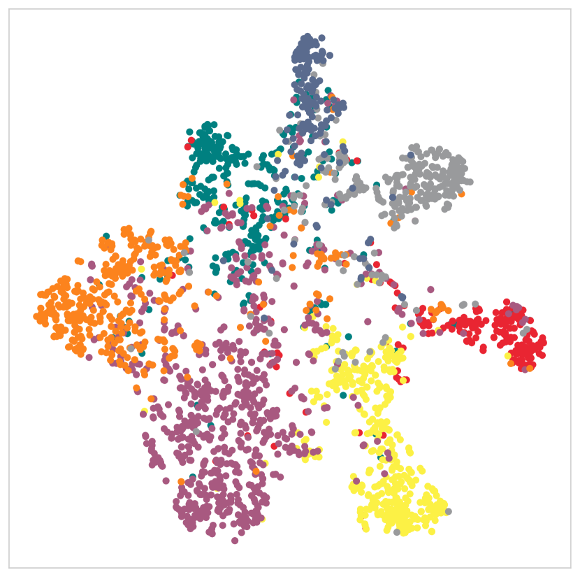
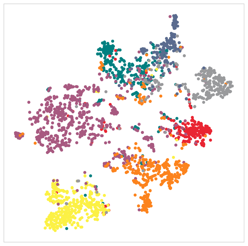
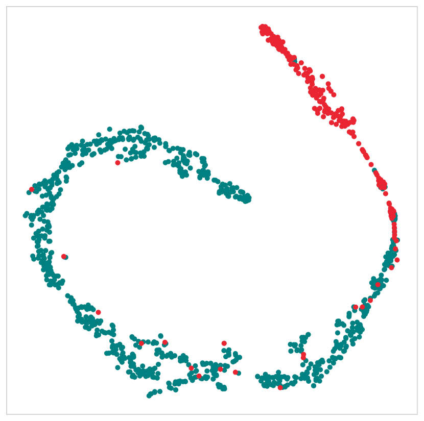
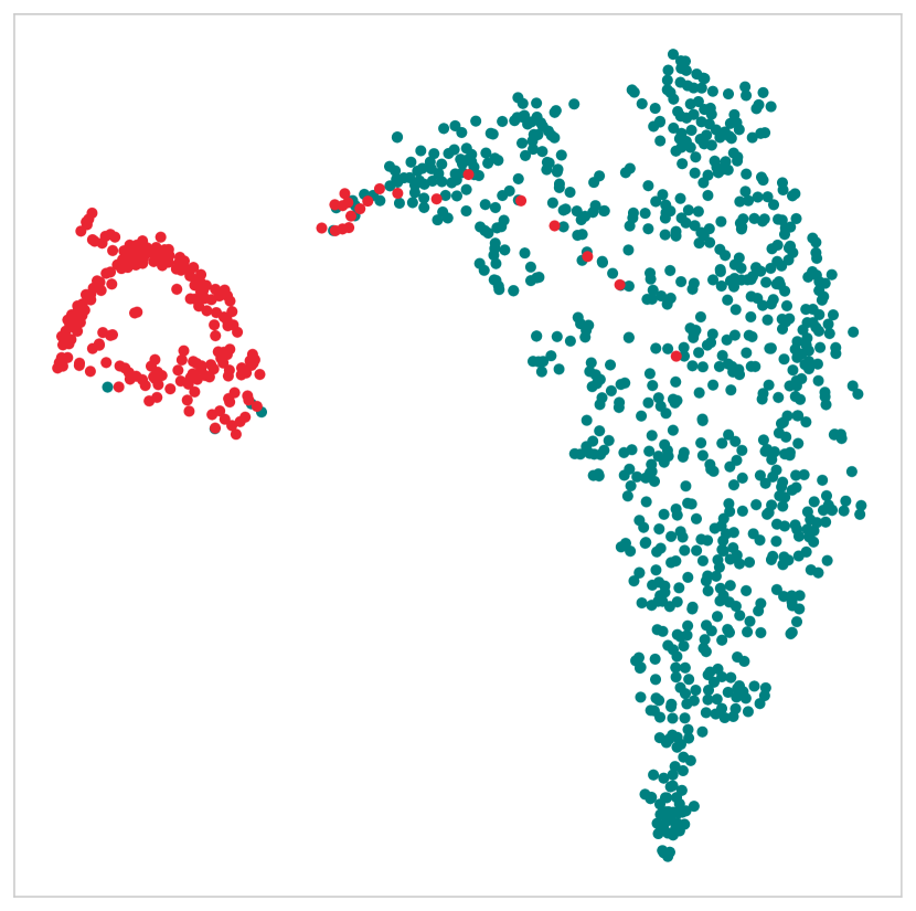
Figure 7. Visualization of Cora and DISEASE. First row: Embedding of Cora by HGCN (left) and $\kappa$HGCN (right)]; Second row: Embedding of DISEASE by HGCN (left) and $\kappa$HGCN (right)

The efficacy of $\kappa$HGCN and HGCN in learning representations for node classification is demonstrated through the visualization of their performance on the Disease and Cora datasets. To accomplish this, we employ the t-distributed Stochastic Neighbor Embedding (t-SNE) technique (Van der Maaten and Hinton, 2008) to reduce the high-dimensional embeddings produced by the final layer of each model to a two-dimensional plane for visual examination. The results, shown in Figure 7, depict nodes as individual points, where each point is assigned a color that corresponds to its class. The visualization indicates that the representations learned by $\kappa$HGCN exhibit sharper boundaries between different classes, thus showcasing the improved discriminative power of the proposed method compared to HGCN.

C.3. Curvature-wise Performance

The objective of the study is to perceive the local structure around nodes in tree-like graphs, encompassing local tree-like, zero-density, and densely connected structures. To demonstrate the effectiveness of the proposed method, we conducted further analysis by classifying nodes into defined local substructures. As an example, consider the following, we set the nodes to the following three types: tree-like $\left(\kappa_{i}\geq-0.01\right)$; zero-like $\left(-0.01<\kappa_{i}\leq 0.01\right)$; positive-like $\left(\kappa_{i}>0.01\right)$. The curvature of each node is defined as the sum of curvatures over its edges, that is: $\kappa_{i}=\frac{1}{\left|N_{i}\right|}\sum_{j\in N_{i}}\kappa_{ij},$ where $\left|N_{i}\right|$ is the number of neighbors of node $i$, and $\kappa_{ij}$ is the curvature of the edge between nodes $i$ and $j$. This curvature measure was used to determine the local substructure of each node. In the following, we evaluated the performance of three models (GCN, HGCN, and the proposed method) on both the Cora and Airport datasets. Specifically, we calculated the accuracy/F1-score on the test set for nodes in each local substructure.

Table 8. Curvature-wise performance on cora dataset

Method	Negative	Zero	Positive
GT-Prop (%)	$\mathbf{0.536}$	$\mathbf{0.138}$	$\mathbf{0.326}$
GCN (%)	0.512	$\mathbf{0.085}$	0.216
HGCN (%)	0.523	0.077	0.213
$\kappa$HGCN (%)	$\mathbf{0.535}$	0.082	$\mathbf{0.217}$

Table 9. Curvature-wise performance on Airport dataset

Method	Negative	Zero	Positive
GT-Prop (%)	$\mathbf{0.418}$	$\mathbf{0.439}$	$\mathbf{0.143}$
GCN (%)	0.277	$\mathbf{0.424}$	0.118
HGCN (%)	0.382	0.405	0.117
$\kappa$HGCN (%)	$\mathbf{0.395}$	0.410	$\mathbf{0.123}$

The results are shown in Table 8 and Table 9. The ”GT-Prop” row in the Tables show the proportion of nodes belonging to each local substructure, with the proportions summing to 1. The values in the GCN, HGCN, and proposed model rows represent the proportion of nodes in each substructure that were correctly predicted by the respective models. In other words, the table presents the accuracy of each model in representing the local environment for different types of nodes. Overall, the study found that the models achieved comparable accuracy to the best achievable, but performance varied across different substructures. Specifically, Euclidean GCN outperformed HGCN on zero-density and densely connected areas, but underperformed on tree-like nodes. In contrast, HGCN showed improved accuracy for tree-like nodes, but lower accuracy on other substructures. The proposed model achieved a balance of performance across all substructures, with high accuracy for both tree-like and non-tree-like nodes.

C.4. Connections of the Discrete and Continuous Curvatures

The discrete curvature $\kappa$ is computed in advance, which can be regarded as an edge weight. The continuous curvature $c$ of the predefined hyperbolic space is learnable and differentiable. For simplicity, we denote the learnable parameters of our model $\kappa$HGCN as $\theta$. Let us consider node classification as an example. If the ground-truth label of node $\mathbf{x}$ is $\mathbf{y}$ and the predicted label is $\bar{\mathbf{y}}$, then we have $\bar{\mathbf{y}}=\textrm{{$\kappa$}HGCN}(\mathbf{x},\kappa,\theta,c)$ and the loss is given by $L({\mathbf{y},\bar{\mathbf{y}}})$. We can take the derivative of $c$ with respect to the loss, i.e., $\frac{\partial L({\mathbf{y},\bar{\mathbf{y}}})}{\partial c}=\frac{\partial(\mathbf{y},\textrm{{$\kappa$}HGCN}(\mathbf{x},\kappa,\theta,c))}{\partial c}$. It is easy to see that the update of $c$ is constrained by $\kappa$. In other words, we learn a good embedding space equipped with curvature $c$ that matches the graph structure through discrete Ricci curvature $\kappa$.

References

- (1)
- Abu-Ata and Dragan (2016) Muad Abu-Ata and Feodor F Dragan. 2016. Metric tree-like structures in real-world networks: an empirical study. Networks 67, 1 (2016), 49–68.
- Ache and Warren (2019) Antonio G Ache and Micah W Warren. 2019. Ricci curvature and the manifold learning problem. Advances in Mathematics 342 (2019), 14–66.
- Adcock et al. (2013) Aaron B Adcock, Blair D Sullivan, and Michael W Mahoney. 2013. Tree-like structure in large social and information networks. In IEEE International Conference on Data Mining. IEEE, 1–10.
- Ambrose et al. (1957) W Ambrose et al. 1957. A theorem of Myers. Duke Mathematical Journal 24, 3 (1957), 345–348.
- Atigh et al. (2022) Mina Ghadimi Atigh, Julian Schoep, Erman Acar, Nanne van Noord, and Pascal Mettes. 2022. Hyperbolic Image Segmentation. In IEEE/CVF Conference on Computer Vision and Pattern Recognition. 4453–4462.
- Bachmann et al. (2020) Gregor Bachmann, Gary Bécigneul, and Octavian Ganea. 2020. Constant curvature graph convolutional networks. In International Conference on Machine Learning. PMLR, 486–496.
- Bai et al. (2023) Qijie Bai, Changli Nie, Haiwei Zhang, Dongming Zhao, and Xiaojie Yuan. 2023. HGWaveNet: A Hyperbolic Graph Neural Network for Temporal Link Prediction. arXiv preprint arXiv:2304.07302 (2023).
- Bai et al. (2021) Yushi Bai, Zhitao Ying, Hongyu Ren, and Jure Leskovec. 2021. Modeling heterogeneous hierarchies with relation-specific hyperbolic cones. Advances in Neural Information Processing Systems 34 (2021), 12316–12327.
- Bouchard et al. (2015) Guillaume Bouchard, Sameer Singh, and Theo Trouillon. 2015. On Approximate Reasoning Capabilities of Low-Rank Vector Spaces.. In AAAI spring symposia.
- Chami et al. (2020) Ines Chami, Adva Wolf, Da-Cheng Juan, Frederic Sala, Sujith Ravi, and Christopher Ré. 2020. Low-Dimensional Hyperbolic Knowledge Graph Embeddings. In Proceedings of the 58th Annual Meeting of the Association for Computational Linguistics. 6901–6914.
- Chami et al. (2019) Ines Chami, Zhitao Ying, Christopher Ré, and Jure Leskovec. 2019. Hyperbolic graph convolutional neural networks. In Advances in Neural Information Processing Systems. 4868–4879.
- Chen et al. (2023a) Yankai Chen, Yixiang Fang, Yifei Zhang, and Irwin King. 2023a. Bipartite Graph Convolutional Hashing for Effective and Efficient Top-N Search in Hamming Space. In Proceedings of the ACM Web Conference. 3164–3172.
- Chen et al. (2022a) Yankai Chen, Huifeng Guo, Yingxue Zhang, Chen Ma, Ruiming Tang, Jingjie Li, and Irwin King. 2022a. Learning binarized graph representations with multi-faceted quantization reinforcement for top-k recommendation. In Proceedings of the 28th ACM SIGKDD Conference on Knowledge Discovery and Data Mining. 168–178.
- Chen et al. (2022c) Yankai Chen, Menglin Yang, Yingxue Zhang, Mengchen Zhao, Ziqiao Meng, Jianye Hao, and Irwin King. 2022c. Modeling scale-free graphs with hyperbolic geometry for knowledge-aware recommendation. In ACM International Conference on Web Search and Data Mining. 94–102.
- Chen et al. (2022b) Yankai Chen, Yaming Yang, Yujing Wang, Jing Bai, Xiangchen Song, and Irwin King. 2022b. Attentive Knowledge-aware Graph Convolutional Networks with Collaborative Guidance for Personalized Recommendation. In ICDE.
- Chen et al. (2023b) Yankai Chen, Yifei Zhang, Menglin Yang, Zixing Song, Chen Ma, and Irwin King. 2023b. WSFE: Wasserstein Sub-graph Feature Encoder for Effective User Segmentation in Collaborative Filtering. arXiv preprint arXiv:2305.04410 (2023).
- Choudhary et al. (2022) Nurendra Choudhary, Nikhil Rao, Karthik Subbian, Srinivasan H Sengamedu, and Chandan K Reddy. 2022. Hyperbolic Neural Networks: Theory, Architectures and Applications. In Proceedings of the 28th ACM SIGKDD Conference on Knowledge Discovery and Data Mining. 4778–4779.
- Cushing et al. (2019) David Cushing, Riikka Kangaslampi, Valtteri Lipiäinen, Shiping Liu, and George W Stagg. 2019. The Graph Curvature Calculator and the curvatures of cubic graphs. Experimental Mathematics (2019), 1–13.
- Cuturi (2013) Marco Cuturi. 2013. Sinkhorn distances: Lightspeed computation of optimal transport. Advances in Neural Information Processing Systems 26 (2013), 2292–2300.
- Dou et al. (2020) Yingtong Dou, Zhiwei Liu, Li Sun, Yutong Deng, Hao Peng, and Philip S Yu. 2020. Enhancing graph neural network-based fraud detectors against camouflaged fraudsters. In ACM International Conference on Information & Knowledge Management. 315–324.
- Forman (2003) Robin Forman. 2003. Bochner’s method for cell complexes and combinatorial Ricci curvature. Discrete and Computational Geometry 29, 3 (2003), 323–374.
- Fu et al. (2023) Xingcheng Fu, Yuecen Wei, Qingyun Sun, Haonan Yuan, Jia Wu, Hao Peng, and Jianxin Li. 2023. Hyperbolic Geometric Graph Representation Learning for Hierarchy-imbalance Node Classification. In Proceedings of the ACM Web Conference 2023. 460–468.
- Fu et al. (2020) Xinyu Fu, Jiani Zhang, Ziqiao Meng, and Irwin King. 2020. MAGNN: Metapath aggregated graph neural network for heterogeneous graph embedding. In Proceedings of the Web Conference. 2331–2341.
- Ganea et al. (2018) Octavian Ganea, Gary Bécigneul, and Thomas Hofmann. 2018. Hyperbolic neural networks. In Advances in Neural Information Processing Systems. 5345–5355.
- Gasteiger et al. (2018) Johannes Gasteiger, Aleksandar Bojchevski, and Stephan Günnemann. 2018. Predict then propagate: Graph neural networks meet personalized pagerank. arXiv preprint arXiv:1810.05997 (2018).
- Gu et al. (2019) Albert Gu, Frederic Sala, Beliz Gunel, and Christopher Ré. 2019. Learning mixed-curvature representations in product spaces. In International Conference on Learning Representations.
- Gulcehre et al. (2018) Caglar Gulcehre, Misha Denil, Mateusz Malinowski, Ali Razavi, Razvan Pascanu, Karl Moritz Hermann, Peter Battaglia, Victor Bapst, David Raposo, Adam Santoro, et al. 2018. Hyperbolic attention networks. arXiv preprint arXiv:1805.09786 (2018).
- Hamilton et al. (2017a) William L Hamilton, Rex Ying, and Jure Leskovec. 2017a. Inductive representation learning on large graphs. In Advances in Neural Information Processing Systems. 1025–1035.
- Hamilton et al. (2017b) William L Hamilton, Rex Ying, and Jure Leskovec. 2017b. Inductive representation learning on large graphs. In Advances in Neural Information Processing Systems. 1025–1035.
- Hsu et al. (2021) Joy Hsu, Jeffrey Gu, Gong Wu, Wah Chiu, and Serena Yeung. 2021. Capturing implicit hierarchical structure in 3D biomedical images with self-supervised hyperbolic representations. Advances in Neural Information Processing Systems 34 (2021), 5112–5123.
- Huang and Zitnik (2020) Kexin Huang and Marinka Zitnik. 2020. Graph meta learning via local subgraphs. Advances in Neural Information Processing Systems 33 (2020).
- Jonckheere et al. (2011) Edmond Jonckheere, Mingji Lou, Francis Bonahon, and Yuliy Baryshnikov. 2011. Euclidean versus hyperbolic congestion in idealized versus experimental networks. Internet Mathematics 7, 1 (2011), 1–27.
- Jost and Liu (2014) Jürgen Jost and Shiping Liu. 2014. Ollivier’s Ricci curvature, local clustering and curvature-dimension inequalities on graphs. Discrete & Computational Geometry 51, 2 (2014), 300–322.
- Khrulkov et al. (2020) Valentin Khrulkov, Leyla Mirvakhabova, Evgeniya Ustinova, Ivan Oseledets, and Victor Lempitsky. 2020. Hyperbolic image embeddings. In IEEE/CVF Conference on Computer Vision and Pattern Recognition. 6418–6428.
- Kipf and Welling (2017) Thomas N Kipf and Max Welling. 2017. Semi-Supervised Classification with Graph Convolutional Networks. In International Conference on Learning Representations.
- Kolyvakis et al. (2019) Prodromos Kolyvakis, Alexandros Kalousis, and Dimitris Kiritsis. 2019. HyperKG: Hyperbolic knowledge graph embeddings for knowledge base completion. arXiv preprint arXiv:1908.04895 (2019).
- Krioukov et al. (2009) Dmitri Krioukov, Fragkiskos Papadopoulos, Amin Vahdat, and Marián Boguná. 2009. Curvature and temperature of complex networks. Physical Review E 80, 3 (2009), 035101.
- Law (2021) Marc Law. 2021. Ultrahyperbolic Neural Networks. In Advances in Neural Information Processing Systems.
- Law and Stam (2020) Marc Law and Jos Stam. 2020. Ultrahyperbolic representation learning. Advances in neural information processing systems 33 (2020), 1668–1678.
- Lee (2018) John M Lee. 2018. Introduction to Riemannian manifolds. Vol. 2. Springer.
- Li et al. (2022) Bisheng Li, Min Zhou, Shengzhong Zhang, Menglin Yang, Defu Lian, and Zengfeng Huang. 2022. BSAL: A Framework of Bi-component Structure and Attribute Learning for Link Prediction. arXiv preprint arXiv:2204.09508 (2022).
- Liu et al. (2022a) Jiahong Liu, Philippe Fournier-Viger, Min Zhou, Ganghuan He, and Mourad Nouioua. 2022a. CSPM: Discovering compressing stars in attributed graphs. Information Sciences 611 (2022), 126–158.
- Liu et al. (2022b) Jiahong Liu, Menglin Yang, Min Zhou, Shanshan Feng, and Philippe Fournier-Viger. 2022b. Enhancing Hyperbolic Graph Embeddings via Contrastive Learning. arXiv preprint arXiv:2201.08554 (2022).
- Liu et al. (2022c) Jiahong Liu, Min Zhou, Philippe Fournier-Viger, Menglin Yang, Lujia Pan, and Mourad Nouioua. 2022c. Discovering Representative Attribute-stars via Minimum Description Length. In 2022 IEEE 38th International Conference on Data Engineering (ICDE). IEEE, 68–80.
- Liu et al. (2019) Qi Liu, Maximilian Nickel, and Douwe Kiela. 2019. Hyperbolic graph neural networks. In Advances in Neural Information Processing Systems. 8230–8241.
- Loisel and Romon (2014) Benoît Loisel and Pascal Romon. 2014. Ricci curvature on polyhedral surfaces via optimal transportation. Axioms 3, 1 (2014), 119–139.
- Lou et al. (2020) Aaron Lou, Isay Katsman, Qingxuan Jiang, Serge Belongie, Ser-Nam Lim, and Christopher De Sa. 2020. Differentiating through the fréchet mean. In International Conference on Machine Learning. PMLR, 6393–6403.
- Ma et al. (2019) Chen Ma, Liheng Ma, Yingxue Zhang, Jianing Sun, Xue Liu, and Mark Coates. 2019. Memory Augmented Graph Neural Networks for Sequential Recommendation. arXiv preprint arXiv:1912.11730 (2019).
- Ma et al. (2021) Xiaoxiao Ma, Jia Wu, Shan Xue, Jian Yang, Chuan Zhou, Quan Z Sheng, Hui Xiong, and Leman Akoglu. 2021. A comprehensive survey on graph anomaly detection with deep learning. IEEE Transactions on Knowledge and Data Engineering (2021).
- Mettes et al. (2023) Pascal Mettes, Mina Ghadimi Atigh, Martin Keller-Ressel, Jeffrey Gu, and Serena Yeung. 2023. Hyperbolic Deep Learning in Computer Vision: A Survey. arXiv preprint arXiv:2305.06611 (2023).
- Montella et al. (2021) Sebastien Montella, Lina M Rojas Barahona, and Johannes Heinecke. 2021. Hyperbolic Temporal Knowledge Graph Embeddings with Relational and Time Curvatures. In Findings of the Association for Computational Linguistics: ACL-IJCNLP 2021. 3296–3308.
- Morris et al. (2019) Christopher Morris, Martin Ritzert, Matthias Fey, William L Hamilton, Jan Eric Lenssen, Gaurav Rattan, and Martin Grohe. 2019. Weisfeiler and leman go neural: Higher-order graph neural networks. In Proceedings of the AAAI Conference on Artificial Intelligence, Vol. 33. 4602–4609.
- Narayan and Saniee (2011) Onuttom Narayan and Iraj Saniee. 2011. Large-scale curvature of networks. Physical Review E 84, 6 (2011), 066108.
- Ni et al. (2018) Chien-Chun Ni, Yu-Yao Lin, Jie Gao, and Xianfeng Gu. 2018. Network alignment by discrete Ollivier-Ricci flow. In International Symposium on Graph Drawing and Network Visualization. Springer, 447–462.
- Ni et al. (2015) Chien-Chun Ni, Yu-Yao Lin, Jie Gao, Xianfeng David Gu, and Emil Saucan. 2015. Ricci curvature of the internet topology. In 2015 IEEE conference on computer communications. IEEE, 2758–2766.
- Nickel and Kiela (2017) Maximillian Nickel and Douwe Kiela. 2017. Poincaré embeddings for learning hierarchical representations. In Advances in Neural Information Processing Systems. 6338–6347.
- Nickel and Kiela (2018) Maximillian Nickel and Douwe Kiela. 2018. Learning Continuous Hierarchies in the Lorentz Model of Hyperbolic Geometry. In International Conference on Machine Learning. 3779–3788.
- Ollivier (2009) Yann Ollivier. 2009. Ricci curvature of Markov chains on metric spaces. Journal of Functional Analysis 256, 3 (2009), 810–864.
- Pal et al. (2017) Siddharth Pal, Feng Yu, Terrence J Moore, Ram Ramanathan, Amotz Bar-Noy, and Ananthram Swami. 2017. An efficient alternative to Ollivier-Ricci curvature based on the Jaccard metric. arXiv preprint arXiv:1710.01724 (2017).
- Peng et al. (2020) Wei Peng, Jingang Shi, Zhaoqiang Xia, and Guoying Zhao. 2020. Mix dimension in poincaré geometry for 3d skeleton-based action recognition. In ACM International Conference on Multimedia (MM). 1432–1440.
- Peng et al. (2021) Wei Peng, Tuomas Varanka, Abdelrahman Mostafa, Henglin Shi, and Guoying Zhao. 2021. Hyperbolic deep neural networks: A survey. IEEE Transactions on Pattern Analysis and Machine Intelligence (2021).
- Sala et al. (2018) Frederic Sala, Chris De Sa, Albert Gu, and Christopher Re. 2018. Representation Tradeoffs for Hyperbolic Embeddings. In International Conference on Machine Learning. 4460–4469.
- Sarkar (2011) Rik Sarkar. 2011. Low distortion delaunay embedding of trees in hyperbolic plane. In International Symposium on Graph Drawing. Springer, 355–366.
- Shavitt and Tankel (2008) Yuval Shavitt and Tomer Tankel. 2008. Hyperbolic embedding of internet graph for distance estimation and overlay construction. IEEE/ACM Transactions on Networking 16, 1 (2008), 25–36.
- Shimizu et al. (2020) Ryohei Shimizu, Yusuke Mukuta, and Tatsuya Harada. 2020. Hyperbolic neural networks++. arXiv preprint arXiv:2006.08210 (2020).
- Song and King (2022) Zixing Song and Irwin King. 2022. Hierarchical Heterogeneous Graph Attention Network for Syntax-Aware Summarization. In Proceedings of the AAAI Conference on Artificial Intelligence, Vol. 36. 11340–11348.
- Song et al. (2021a) Zixing Song, Ziqiao Meng, Yifei Zhang, and Irwin King. 2021a. Semi-supervised Multi-label Learning for Graph-structured Data. In ACM International Conference on Information & Knowledge Management. 1723–1733.
- Song et al. (2021b) Zixing Song, Xiangli Yang, Zenglin Xu, and Irwin King. 2021b. Graph-based semi-supervised learning: A comprehensive review. arXiv preprint arXiv:2102.13303 (2021).
- Song et al. (2022) Zixing Song, Yifei Zhang, and Irwin King. 2022. Towards an optimal asymmetric graph structure for robust semi-supervised node classification. In Proceedings of the ACM SIGKDD Conference on Knowledge Discovery and Data Mining. 1656–1665.
- Sun et al. (2021) Jianing Sun, Zhaoyue Cheng, Saba Zuberi, Felipe Pérez, and Maksims Volkovs. 2021. HGCF: Hyperbolic Graph Convolution Networks for Collaborative Filtering. In Proceedings of the Web Conference. 593–601.
- Sun et al. (2022) Li Sun, Zhongbao Zhang, Junda Ye, Hao Peng, Jiawei Zhang, Sen Su, and Philip S Yu. 2022. A Self-supervised Mixed-curvature Graph Neural Network. Proceedings of the AAAI Conference on Artificial Intelligence (2022).
- Suzuki et al. (2021a) Atsushi Suzuki, Atsushi Nitanda, Jing Wang, Linchuan Xu, Kenji Yamanishi, and Marc Cavazza. 2021a. Generalization error bound for hyperbolic ordinal embedding. In International Conference on Machine Learning. PMLR, 10011–10021.
- Suzuki et al. (2021b) Atsushi Suzuki, Atsushi Nitanda, Linchuan Xu, Kenji Yamanishi, Marc Cavazza, et al. 2021b. Generalization bounds for graph embedding using negative sampling: Linear vs hyperbolic. Advances in Neural Information Processing Systems 34 (2021), 1243–1255.
- Topping et al. (2021) Jake Topping, Francesco Di Giovanni, Benjamin Paul Chamberlain, Xiaowen Dong, and Michael M Bronstein. 2021. Understanding over-squashing and bottlenecks on graphs via curvature. arXiv preprint arXiv:2111.14522 (2021).
- Ungar et al. (2007) Abraham A Ungar et al. 2007. The hyperbolic square and mobius transformations. Banach Journal of Mathematical Analysis 1, 1 (2007), 101–116.
- Van der Hoorn et al. (2020) Pim Van der Hoorn, Gabor Lippner, Carlo Trugenberger, et al. 2020. Ollivier curvature of random geometric graphs converges to Ricci curvature of their Riemannian manifolds. arXiv preprint arXiv:2009.04306 (2020).
- Van der Maaten and Hinton (2008) Laurens Van der Maaten and Geoffrey Hinton. 2008. Visualizing data using t-SNE. JMLR 9, 11 (2008).
- Veličković et al. (2018) Petar Veličković, Guillem Cucurull, Arantxa Casanova, Adriana Romero, Pietro Liò, and Yoshua Bengio. 2018. Graph Attention Networks. In International Conference on Learning Representations.
- Verbeek and Suri (2014) Kevin Verbeek and Subhash Suri. 2014. Metric embedding, hyperbolic space, and social networks. In Proceedings of the thirtieth annual symposium on Computational geometry. 501–510.
- Vinh Tran et al. (2020) Lucas Vinh Tran, Yi Tay, Shuai Zhang, Gao Cong, and Xiaoli Li. 2020. HyperML: A Boosting Metric Learning Approach in Hyperbolic Space for Recommender Systems. In ACM International Conference on Web Search and Data Mining. New York, NY, USA, 609–617.
- Wang et al. (2021a) Hao Wang, Defu Lian, Hanghang Tong, Qi Liu, Zhenya Huang, and Enhong Chen. 2021a. HyperSoRec: Exploiting Hyperbolic User and Item Representations with Multiple Aspects for Social-aware Recommendation. TOIS (2021), 1–28.
- Wang et al. (2021b) Shen Wang, Xiaokai Wei, Cicero Nogueira Nogueira dos Santos, Zhiguo Wang, Ramesh Nallapati, Andrew Arnold, Bing Xiang, Philip S Yu, and Isabel F Cruz. 2021b. Mixed-curvature multi-relational graph neural network for knowledge graph completion. In Proceedings of the Web Conference. 1761–1771.
- Wu et al. (2019) Felix Wu, Amauri Souza, Tianyi Zhang, Christopher Fifty, Tao Yu, and Kilian Weinberger. 2019. Simplifying graph convolutional networks. In International Conference on Machine Learning. PMLR, 6861–6871.
- Xiong et al. (2022a) Bo Xiong, M. Cochez, Mojtaba Nayyeri, and Steffen Staab. 2022a. Hyperbolic Embedding Inference for Structured Multi-Label Prediction. In Proceedings of the 36th Conference on Neural Information Processing Systems.
- Xiong et al. (2022b) Bo Xiong, Shichao Zhu, Mojtaba Nayyeri, Chengjin Xu, Shirui Pan, Chuan Zhou, and Steffen Staab. 2022b. Ultrahyperbolic knowledge graph embeddings. In Proceedings of the 28th ACM SIGKDD Conference on Knowledge Discovery and Data Mining. 2130–2139.
- Xiong et al. (2021) Bo Xiong, Shichao Zhu, Nico Potyka, Shirui Pan, Chuan Zhou, and Steffen Staab. 2021. Pseudo-Riemannian Graph Convolutional Networks. arXiv preprint arXiv:2106.03134 (2021).
- Yang et al. (2022a) Menglin Yang, Zhihao Li, Min Zhou, Jiahong Liu, and Irwin King. 2022a. HICF: Hyperbolic informative collaborative filtering. In Proceedings of the 28th ACM SIGKDD Conference on Knowledge Discovery and Data Mining. 2212–2221.
- Yang et al. (2020) Menglin Yang, Ziqiao Meng, and Irwin King. 2020. FeatureNorm: L2 Feature Normalization for Dynamic Graph Embedding. In IEEE International Conference on Data Mining. 731–740.
- Yang et al. (2021) Menglin Yang, Min Zhou, Marcus Kalander, Zengfeng Huang, and Irwin King. 2021. Discrete-time Temporal Network Embedding via Implicit Hierarchical Learning in Hyperbolic Space. In Proceedings of the ACM SIGKDD Conference on Knowledge Discovery and Data Mining. 1975–1985.
- Yang et al. (2022b) Menglin Yang, Min Zhou, Zhihao Li, Jiahong Liu, Lujia Pan, Hui Xiong, and Irwin King. 2022b. Hyperbolic Graph Neural Networks: A Review of Methods and Applications. arXiv preprint arXiv:2202.13852 (2022).
- Yang et al. (2022c) Menglin Yang, Min Zhou, Jiahong Liu, Defu Lian, and Irwin King. 2022c. HRCF: Enhancing Collaborative Filtering via Hyperbolic Geometric Regularization. In Proceedings of the Web Conference.
- Yang et al. (2022d) Menglin Yang, Min Zhou, Hui Xiong, and Irwin King. 2022d. Hyperbolic Temporal Network Embedding. IEEE Transactions on Knowledge and Data Engineering (2022).
- Ye et al. (2019) Ze Ye, Kin Sum Liu, Tengfei Ma, Jie Gao, and Chao Chen. 2019. Curvature Graph Network. In International Conference on Learning Representations.
- Zhang et al. (2020) Kai Zhang, Yaokang Zhu, Jun Wang, and Jie Zhang. 2020. Adaptive structural fingerprints for graph attention networks. In International Conference on Learning Representations.
- Zhang and Chen (2018) Muhan Zhang and Yixin Chen. 2018. Link prediction based on graph neural networks. Advances in Neural Information Processing Systems 31 (2018).
- Zhang et al. (2021a) Yiding Zhang, Xiao Wang, Chuan Shi, Xunqiang Jiang, and Yanfang Fanny Ye. 2021a. Hyperbolic graph attention network. IEEE Transactions on Big Data (2021).
- Zhang et al. (2021b) Yiding Zhang, Xiao Wang, Chuan Shi, Nian Liu, and Guojie Song. 2021b. Lorentzian Graph Convolutional Networks. In Proceedings of the Web Conference. 1249–1261.
- Zhang et al. (2022a) Yifei Zhang, Hao Zhu, Ziqiao Meng, Piotr Koniusz, and Irwin King. 2022a. Graph-adaptive rectified linear unit for graph neural networks. In Proceedings of the Web Conference. 1331–1339.
- Zhang et al. (2022b) Yifei Zhang, Hao Zhu, Zixing Song, Piotr Koniusz, and Irwin King. 2022b. COSTA: Covariance-Preserving Feature Augmentation for Graph Contrastive Learning. In Proceedings of the ACM SIGKDD Conference on Knowledge Discovery and Data Mining. 2524–2534.
- Zhang et al. (2022c) Yifei Zhang, Hao Zhu, Zixing Song, Piotr Koniusz, and Irwin King. 2022c. Spectral Feature Augmentation for Graph Contrastive Learning and Beyond. arXiv preprint arXiv:2212.01026 (2022).
- Zhou et al. (2022a) Min Zhou, Bisheng Li, Menglin Yang, and Lujia Pan. 2022a. TeleGraph: A benchmark dataset for hierarchical link prediction. arXiv preprint arXiv:2204.07703 (2022).
- Zhou et al. (2022b) Min Zhou, Menglin Yang, Lujia Pan, and Irwin King. 2022b. Hyperbolic Graph Representation Learning: A Tutorial. arXiv preprint arXiv:2211.04050 (2022).
- Zhu et al. (2020) Shichao Zhu, Shirui Pan, Chuan Zhou, Jia Wu, Yanan Cao, and Bin Wang. 2020. Graph Geometry Interaction Learning. In Advances in Neural Information Processing Systems, Vol. 33.