Inflationary Cosmology in a non-minimal $f(R,T)$ gravity theory using a $RT$ mixing term

Abstract

We investigate a class of inflationary models in modified gravity theories which contain a non-minimal coupling between gravity and a scalar field $\phi$ (inflaton) as $f(R,T)=R\bigl{(}1+\alpha+\kappa^{4}\beta T\bigr{)}+\kappa^{2}\gamma T$ where $\kappa^{2}=8\pi G$ where $G$ is the Newton’s constant. We consider two inflaton potentials of the form (i) $V=V_{0}\bigl{(}1+\ln{\phi}\bigr{)}$ and (ii) $V_{0}\frac{\lambda\phi^{p}}{1+\lambda\phi^{p}}$. For a range of potential parameters, we explored the constraints on modified gravity parameters i.e. ($\alpha$, $\beta$ and $\gamma$) in three categories — (i) $\beta\neq 0$, $\alpha=\gamma=0$ (considering $R$ and $RT$ mixing terms), (ii) $\alpha=0$, $\gamma\neq 0$, $\beta\neq 0$ ($RT$ mixing term along with $T$ and $R$ terms) and (iii) $\gamma=0$, $\alpha\neq 0$, $\beta\neq 0$ ($RT$ mixing term along with $R$ term) for the above two potentials. The inclusion of $RT$ mixing term provides the scalar spectral index $n_{s}$ up to $3\sigma$ limit of PLANCK data, which is $n_{s}=0.9649\pm 0.0042$ as well as the tensor-to-scalar ratio $r<0.106$ and the e-fold parameter $40<N<70$ for both the potentials.

Payel Sarkar, Ashmita, Prasanta Kumar Das

Keywords: Inflation, Non-minimal coupling, $RT$-mixing term, spectral index parameters.

1 Introduction

Although the history of the observable universe prior to the era of nucleosynthesis is unknown, it is commonly accepted that cosmic inflation occurred just after the Big Bang. It is a theory of exponential accelerated expansion of the universe, first envisioned by A. Guth in 1981 [1, 2], when the entire observable universe, once contained in a tiny region of the Universe all at the same temperature, suddenly expanded (in a brief fraction of a second).
Inflation, which solves cosmological problems such as flatness problem, and horizon problem [3, 4], is a hot research topic in modern cosmology. It helps us to understand “why the observable universe today is so much isotropic and homogeneous?” Inflation also acts as the seed of density fluctuations and CMB anisotropies [3, 5], which later evolve as Large scale structures of our universe. The scale invariant cosmological perturbations arose due to the density fluctuations, agree remarkably well with observational data such as COBE[6], BICEP[7], PLANCK[8] and WMAP[9]. The WMAP data measures the spectral index of the scalar fluctuations $n_{s}=0.99\pm 0.04$ and put the $95\%$ C.L. upper limit on the tensor-to-scalar ratio, $r<0.9$. The recent PLANCK-2018 mission measures the scalar spectral index $n_{s}=0.9649\pm 0.0042$ and put the upper limit on $r<0.1$ (at $95\%$ C.L.), which is further tightened by combining with the BICEP2/Keck Array BK15 data to obtain $r<0.056$.
Normally, an accepted model of Inflation requires a scalar field in a flat potential, which rolls slowly over the potential for a sufficiently long period of time[4, 10, 11, 12, 13, 14, 15]. But the tightly constrained tensor-to-scalar ratio $r$ rules out many such inflationary models. Besides, a viable inflationary model has to produce the necessary e-fold($N$) to trigger inflation and predict a smaller tensor-scalar ratio $r$ in order to fit with the observational data.
The simplest extension of the scalar field Lagrangian is to introduce a coupling between scalar matter and gravity. The non-minimal inflation model describes the cosmic expansion with a graceful exit [16] towards its end [17, 18]. It is also intriguing to consider a non-minimal coupling scenario in the context of multidimensional theories like super-string theory [19] and induced gravity [20]. In presence of non-minimal matter-gravity term, the conservation equation may not be valid anymore and the extra term in energy-momentum leads to an irreversible particle creation process, which appears in quantum field theory in curved space-time[21, 22, 23, 24, 25, 26, 27, 28]. The addition of non-minimal matter-gravity coupling in modified gravity theory is widely investigated nowadays to explain the late-time acceleration by making use of matter-gravity coupling without introducing any dark matter component.
A host of modified gravity have been studied such as $f(R,T)$ gravity [29, 30], $f(R)$gravity[31, 32, 33], $f(R,\mathcal{L}_{m})$ gravity [34, 35], $f(\phi,T)$[37, 38] along this direction. In this manuscript, we have mentioned two different types of inflationary models in modified $f(R,T)$ gravity where $T$ (the trace of energy-momentum tensor) is coupled with the Ricci scalar $R$. We have taken a modified gravity model with $f(R,T)=R(1+\alpha+\kappa^{4}\beta T)+\kappa^{2}\gamma T$[36] to study inflationary expansion. Here $\alpha,\beta$ and $\gamma$ are the modified gravity parameters which will be estimated using WMAP and PLANCK 2018 data for both the models using a class of inflaton potentials. Chaotic and natural inflation models have also been studied using the aforementioned functional form of $f(R,T)$[36], but no such work has been done for fractional and logarithmic inflaton potential.
In this work, we have considered logarithmic and fractional potential having the form (i) $V=V_{0}(1+\ln{\phi})$ and (ii) $V=V_{0}\frac{\lambda\phi^{p}}{1+\lambda\phi^{p}}$. The analysis of the slow-roll inflation for $V=V_{0}\frac{\lambda\phi^{p}}{1+\lambda\phi^{p}}$ has been reported by these authors in their earlier works [15, 39, 40] for $f(R,T)$ gravity with both linear and higher order term of $T$ and for non-minimal coupling term $\frac{1}{2}\xi R\phi^{2}$ whereas the potential $V=V_{0}(1+\ln{\phi})$ have been discussed in [14] to study inflation. Hence to, study the inflationary expansion in modified gravity theory with the $RT$ mixing term for the above two potentials, is a worthwhile exercise.
The paper is organized as follows. In section 2, we obtain the Einstein Field equations in the modified $f(R,T)$ gravity and derive the potential slow-roll parameters in this $f(R,T)$ gravity. In section 3, we discuss the inflationary scenario for two different potentials and derive the cosmological parameters such as scalar spectral index $n_{s}$ and tensor-to-scalar ratio $r$. These cosmological parameters have been subject to constraints in the parameter space of inflaton potential $(\lambda,p)$ within the context of modified $f(R,T)$ gravity. We analyze our results and compare those with the PLANCK 2018[8] and the WMAP[9] data. In section 4, we briefly summarize our results and conclude.

2 Field equations in modified gravity with RT mixing term

In this modified gravity model where the inflaton field couples non-minimally with gravity, the action is given by,

$$\mathcal{S}=\int d^{4}x\sqrt{-g}\left[\frac{f(R,T)}{2\kappa^{2}}+\mathcal{L}_{m}\right]$$ (1)

where $\kappa^{2}=8\pi G=\frac{1}{M_{Pl}^{2}}$ , $g$ is the determinant of $g_{\mu\nu}$, $R$ is Ricci scalar and $T$ is the trace of energy-momentum tensor $T_{\mu\nu}$. The form of $f(R,T)$ considered here as

$$f(R,T)=R\bigl{(}1+\alpha+\kappa^{4}\beta T\bigr{)}+\kappa^{2}\gamma T$$

where $\alpha,~{}\beta$ and $\gamma$ are the modified gravity parameters. One can recover the Einstein gravity by taking the limit $\alpha,\beta,\gamma$ $\rightarrow 0$. The energy-momentum tensor of the scalar field can be written as,

$$T_{\mu\nu}=\partial_{\mu}\phi\partial_{\nu}\phi+g_{\mu\nu}\mathcal{L}_{m}$$ (2)

where $\mathcal{L}_{m}=-\frac{1}{2}g^{\mu\nu}\partial_{\mu}\phi\partial_{\nu}\phi-V(\phi)$ is the Lagrangian of the scalar field, $V(\phi)$ is the scalar potential. By varying the action (i.e. Eq. (1)) with respect to metric $g_{\mu\nu}$, the modified Einstein field equations can be obtained as

$$f_{R}R_{\mu\nu}-\frac{1}{2}fg_{\mu\nu}+\bigl{(}g_{\mu\nu}\square-\nabla_{\mu}\nabla_{\nu}\bigr{)}f_{R}=T_{\mu\nu}-f_{T}\bigl{(}T_{\mu\nu}+\Theta_{\mu\nu}\bigr{)}$$ (3)

Here $f_{R}=\partial f/\partial R$, $f_{T}=\partial f/\partial T$ and $\Box=\nabla_{\mu}\nabla^{\mu}$, where $\nabla_{\mu}$ is the covariant derivative. The tensor $\Theta_{\mu\nu}$ is defined in terms of the energy-momentum tensor as,

$$\Theta_{\mu\nu}=g^{\lambda\kappa}\frac{\delta T_{\lambda\kappa}}{\delta g^{\mu\nu}}=-T_{\mu\nu}-\partial_{\mu}\phi\partial_{\nu}\phi$$ (4)

Using the above form of $f(R,T)$, the modified Einstein equation can be written as,

$$R_{\mu\nu}-\frac{1}{2}Rg_{\mu\nu}=T_{\mu\nu}^{eff}$$ (5)

where $T_{\mu\nu}^{eff}$, the effective energy-momentum tensor, is given by

$$T_{\mu\nu}^{eff}=T_{\mu\nu}+\bigl{(}R\beta+\gamma\bigr{)}\partial_{\mu}\phi\partial_{\nu}\phi-R_{\mu\nu}\bigl{(}\alpha+\beta T\bigr{)}+\frac{1}{2}g_{\mu\nu}\Bigl{\{}R\bigl{(}\alpha+\beta T\bigr{)}+\gamma T\Bigr{\}}-\bigl{(}g_{\mu\nu}\square-\nabla_{\mu}\nabla_{\nu}\bigr{)}\beta T$$ (6)

Accordingly, the effective energy density and the effective pressure can be derived from the energy-momentum tensor as,

$$\rho^{eff}=\frac{1}{2}\dot{\phi}^{2}\Bigl{(}1+12\beta\dot{H}+\gamma+18\beta H^{2}\Bigr{)}+V\Bigl{(}1+2\gamma+12\beta H^{2}\Bigr{)}-3\alpha H^{2}-6H\beta\dot{\phi}\ddot{\phi}+12\beta H\dot{\phi}V_{,\phi}$$ (7)

and

$$\begin{split}p^{eff}=&\frac{1}{2}\dot{\phi}^{2}\Bigl{(}1+\gamma+4\beta\dot{H}+6\beta H^{2}\Bigr{)}-V\Bigl{(}1+2\gamma+8\beta\dot{H}+12\beta H^{2}\Bigr{)}+2\alpha\dot{H}+3\alpha H^{2}+\beta\Bigl{(}2\ddot{\phi}^{2}+2\dot{\phi}\dddot{\phi}\\ &-4\ddot{\phi}V_{,\phi}-4V_{,\phi\phi}\dot{\phi}^{2}+4H\dot{\phi}\ddot{\phi}-8H\dot{\phi}V_{,\phi}\Bigr{)}\end{split}$$ (8)

Solving the Einstein field equation, Eq. (5) along with Eq. (6), we obtain the modified Friedmann equation and acceleration equation as

$$3H^{2}\bigl{(}1+\alpha\bigr{)}=\frac{1}{2}\dot{\phi}^{2}\bigl{(}1+12\beta\dot{H}+\gamma+18\beta H^{2}\bigr{)}+V\bigl{(}1+2\gamma+12\beta H^{2}\bigr{)}$$ (9)

$$\begin{split}\frac{\ddot{a}}{a}\bigl{(}1+\alpha\bigr{)}=&-\frac{1}{3}\biggl{\{}\dot{\phi}^{2}\Bigl{(}1+\gamma+6\beta\dot{H}-6\beta V_{,\phi\phi}+9\beta H^{2}\Bigr{)}-V\Bigl{(}1+2\gamma+12\beta\dot{H}+12\beta H^{2}\Bigr{)}\biggr{\}}\\ &\qquad-\beta H\dot{\phi}\ddot{\phi}+2\beta H\dot{\phi}V_{,\phi}-\beta\ddot{\phi}^{2}-\beta\dot{\phi}\dddot{\phi}+2\beta\ddot{\phi}V_{,\phi}\end{split}$$ (10)

Furthermore, the equation of continuity of the inflaton takes the form:

$$\ddot{\phi}\Bigl{(}1+\gamma+6\beta\dot{H}+12\beta H^{2}\Bigr{)}+V_{,\phi}\Bigl{(}1+2\gamma+12\beta\dot{H}+24\beta H^{2}\Bigr{)}+3H\dot{\phi}\Bigl{(}1+\gamma+10\beta H^{2}+8\beta\dot{H}\Bigr{)}+6\beta\dot{\phi}\frac{\dddot{a}}{a}=0$$ (11)

In the limit $\alpha\to 0$, $\beta\to 0$ and $\gamma\to 0$, the above set of modified equations take the form

$$3H^{2}=\frac{1}{2}\dot{\phi}^{2}+V(\phi),~{}~{}\frac{\ddot{a}}{a}=-\frac{1}{3}\Biggl{[}\dot{\phi}^{2}-V\Biggr{]}\rm{and}~{}~{}\ddot{\phi}+3H\dot{\phi}+V_{,\phi}=0$$

These are the Friedmann, acceleration and continuity equations in Einstein gravity with a scalar field.

2.1 Inflation: Slow-roll conditions

The slow-roll conditions required for inflationary expansion, are listed as follows

$$\dot{\phi}^{2}<<V(\phi),|\dddot{\phi}|<<|H\ddot{\phi}|<<|H^{2}\dot{\phi}|,~{}~{}|\ddot{H}|<<|H\dot{H}|<<|H^{3}|$$

Applying these conditions, we can approximate Eq. (9) and Eq. (10) as,

$$H^{2}\approx\frac{V}{3}\Biggl{[}\frac{1+2\gamma}{1+\alpha-4\beta V}\Biggr{]}$$ (12)

and

$$\dot{H}\approx-\frac{1}{2}\dot{\phi}^{2}\Biggl{[}\frac{(1+\alpha)(1+\gamma)+4\beta V\gamma}{(1+\alpha-4\beta V)^{2}}\Biggr{]}$$ (13)

and the equation of continuity (Eq. 11) as

$$3H\dot{\phi}\Bigl{\{}(1+\gamma)(1+\alpha)+4\beta V\gamma\Bigr{\}}+V_{,\phi}(1+2\gamma)(1+\alpha+4\beta V)\approx 0$$ (14)

Next, we are to write all the above three equations in the Einstein frame. We use three conformal transformations to do that, which are $\Omega_{1}(\phi),~{}\Omega_{2}(\phi)$ and $\Omega_{3}(\phi)$, respectively on the metric $g_{\mu\nu}$, the inflaton field $\phi$ and the inflaton potential $V(\phi)$.
The first conformal transformation $\Omega_{1}(\phi)$ stands for transformation of metric $g_{\mu\nu}$ to an auxiliary metric $\tilde{g}_{\mu\nu}$ as,

$$\tilde{g}_{\mu\nu}=\Omega_{1}(\phi)g_{\mu\nu}$$ (15)

The line element can be represented as,

$$\tilde{g}_{\mu\nu}dx^{\mu}dx^{\nu}=-d\tilde{t}^{2}+\tilde{a}(\tilde{t})^{2}d\vec{x}^{2}=\Omega_{1}(\phi)\left(-dt^{2}+a^{2}(t)d\vec{x}^{2}\right)$$ (16)

The second scalar field transformation $\Omega_{2}(\phi)$, which transforms $\phi$ to an auxiliary scalar field $\tilde{\phi}$, is defined as,

$$\Biggl{[}\frac{d\tilde{\phi}}{d\phi}\Biggr{]}^{2}=\Omega_{2}(\phi)$$ (17)

And finally, the third transformation $\Omega_{3}(\phi)$ is used for the transformation of the scalar potential and it is defined as

$$\tilde{V}(\tilde{\phi})=\Omega_{3}(\phi)V(\phi)$$ (18)

Applying theses transformations on the metric, the scalar field, and the scalar potential, we can write Eqs.(12), (13) and (14) in the Einstein frame as,

$$\tilde{H}^{2}\Omega_{1}(1+\alpha-4\beta V)=\frac{V}{3}(1+2\gamma)\longrightarrow 3\tilde{H}^{2}\approx\tilde{V}$$ (19)

$$\dot{\tilde{H}}\Omega_{1}(1+\alpha-4\beta V)=-\frac{1}{2}\dot{\phi}^{2}\Biggl{[}\frac{(1+\alpha)(1+\gamma)+4\beta V\gamma}{1+\alpha-4\beta V}\Biggr{]}\longrightarrow\frac{d\tilde{H}}{d\tilde{t}}\approx-\frac{1}{2}\Biggl{[}\frac{d\tilde{\phi}}{d\tilde{t}}\Biggr{]}^{2}$$ (20)

$$3\tilde{H}\frac{d\tilde{\phi}}{d\tilde{t}}+\tilde{V}_{,\tilde{\phi}}\approx 0$$ (21)

where $\tilde{V}_{,\tilde{\phi}}=\frac{d\tilde{V}}{d\tilde{\phi}}$ and $\tilde{H}=\frac{\dot{\tilde{a}}}{\tilde{a}}=H\Omega_{1}^{-1/2}$, $\dot{H}=\Omega_{1}\dot{\tilde{H}},~{}\dot{\phi}=\frac{d\tilde{\phi}}{d\tilde{t}}\Omega_{1}^{1/2}\Omega_{2}^{-1/2}$. The above set of equations can be obtained by choosing

$$\Omega_{1}=1+\alpha-4\beta V$$ (22)

$$\Omega_{2}=\frac{(1+\alpha)(1+\gamma)+4\beta\gamma V}{(1+\alpha-4\beta V)^{2}}$$ (23)

and,

$$\Omega_{3}=\frac{1+2\gamma}{(1+\alpha-4\beta V)^{2}}$$ (24)

In Einstein frame, the potential slow roll parameters can be defined as,

$$\tilde{\epsilon}_{v}=\frac{1}{2}\Biggl{[}\frac{\tilde{V}^{\prime}(\tilde{\phi})}{\tilde{V}(\tilde{\phi})}\Biggr{]}^{2},~{}~{}\tilde{\eta}_{v}=\frac{\tilde{V}^{{}^{\prime\prime}}(\tilde{\phi})}{\tilde{V}(\tilde{\phi})}$$ (25)

where

$$\tilde{V}^{\prime}(\tilde{\phi})=\frac{d\tilde{V}}{d\tilde{\phi}}=V_{,\phi}\Omega_{3}\Omega_{2}^{-1/2},~{}~{}\tilde{V}^{\prime\prime}(\tilde{\phi})=\frac{d^{2}\tilde{V}}{d\tilde{\phi}^{2}}=V_{,\phi\phi}\frac{\Omega_{3}}{\Omega_{2}}+V_{,\phi}\frac{1}{\Omega_{2}}\frac{d\Omega_{3}}{d\phi}-V_{,\phi}\frac{\Omega_{3}}{2\Omega_{2}^{2}}\frac{d\Omega_{2}}{d\phi}$$

The slow-roll parameters are related to the CMBR observables - the scalar spectral index($n_{s}$), tensor spectral index($n_{T}$) and tensor-to scalar ratio($r$) as follows,

$$n_{s}-1=2\tilde{\eta}_{v}-6\tilde{\epsilon}_{v},~{}~{}r=16\tilde{\epsilon}_{v}$$ (26)

The e-fold number $N$ is defined as the ratio of the final value of the scale factor $a_{f}$ during the inflationary era and its initial value $a_{i}$ can be calculated as,

$$N=\int_{\tilde{a_{i}}}^{\tilde{a_{f}}}\frac{d\tilde{a}}{\tilde{a}}=\int_{\tilde{\phi_{i}}}^{\tilde{\phi_{f}}}\frac{\tilde{H}}{d\tilde{\phi}/d\tilde{t}}d\tilde{\phi}=\int_{\phi_{i}}^{\phi_{f}}\frac{H}{\dot{\phi}}d\phi$$ (27)

3 Different Inflationary models

3.1 Model I: $V=V_{0}\bigl{(}1+\ln{\phi}\bigr{)}$: Results and Analysis

First, we consider the inflaton potential of the form,

$$V=V_{0}\bigl{(}1+\ln{\phi}\bigr{)}$$ (28)

where $\phi$ is in unit of $M_{Pl}$, $V_{0}$ is a constant expressed in units of $M_{Pl}^{4}$. This potential was studied by Lyth and Riotto in [41] and is called “Spontaneous broken SUSY Inflation”. Apart from this, the aforementioned potential is also examined by Guo and Zhang [42], Hebecker et al.[43]. The slow-roll parameters for the given potential is

$$\epsilon_{\tilde{V}}=\frac{1}{2\Bigl{\{}\bigl{(}1+\alpha\bigr{)}\bigl{(}1+\gamma\bigr{)}+4\beta V_{0}\bigl{(}1+\ln{\phi}\bigr{)}\Bigr{\}}}\times\Biggl{[}\frac{1+\alpha-4\beta V_{0}(1+\ln{\phi})}{\phi\bigl{(}1+\ln{\phi}\bigr{)}}\Biggr{]}^{2}$$ (29)

$$\begin{split}\eta_{\tilde{V}}&=-\frac{\Bigr{\{}1+\alpha-4\beta V_{0}\bigl{(}1+\ln{\phi}\bigr{)}\Bigr{\}}}{\phi^{2}\bigl{(}1+\ln{\phi}\bigr{)}\Bigl{\{}\bigl{(}1+\alpha\bigr{)}\bigl{(}1+\gamma\bigr{)}+4\beta V_{0}\bigl{(}1+\ln{\phi}\bigr{)}\Bigr{\}}^{2}}\times\Biggl{[}\bigl{(}\alpha+1\bigr{)}^{2}\bigl{(}\gamma+1\bigr{)}-2\beta V_{0}\bigl{(}\alpha+1\bigr{)}\bigl{(}2\gamma\ln{\phi}\\ &\qquad+4\gamma+1\bigr{)}-8\beta^{2}V_{0}^{2}\bigl{(}2{\ln{\phi}}^{2}+7\ln{\phi}+5\bigr{)}\Biggr{]}\end{split}$$ (30)

The spectral index parameters are defined as follows:

$$\begin{split}n_{s}&=1-\frac{3\Bigl{\{}1+\alpha-4\beta V_{0}(1+\ln{\phi})\Bigr{\}}^{2}}{\phi^{2}\bigl{(}1+\ln{\phi}\bigr{)}^{2}\Bigl{\{}\bigl{(}1+\alpha\bigr{)}\bigl{(}1+\gamma\bigr{)}+4\beta V_{0}\bigl{(}1+\ln{\phi}\bigr{)}\Bigr{\}}}-\frac{2\Bigr{\{}1+\alpha-4\beta V_{0}\bigl{(}1+\ln{\phi}\bigr{)}\Bigr{\}}}{\phi^{2}\bigl{(}1+\ln{\phi}\bigr{)}\Bigl{\{}\bigl{(}1+\alpha\bigr{)}\bigl{(}1+\gamma\bigr{)}+4\beta V_{0}\bigl{(}1+\ln{\phi}\bigr{)}\Bigr{\}}^{2}}\\ &\qquad\times\Biggl{[}\bigl{(}\alpha+1\bigr{)}^{2}\bigl{(}1+\gamma\bigr{)}-2\beta V_{0}\bigl{(}1+\alpha\bigr{)}\bigl{(}1+4\gamma+2\gamma\ln{\phi}\bigr{)}-8\beta^{2}V_{0}^{2}\bigl{(}5+7\ln{\phi}+2{\ln{\phi}}^{2}\bigr{)}\Biggr{]}\end{split}$$ (31)

$$r=\frac{8}{\Bigl{\{}\bigl{(}1+\alpha\bigr{)}\bigl{(}1+\gamma\bigr{)}+4\beta V_{0}\bigl{(}1+\ln{\phi}\bigr{)}\Bigr{\}}}\times\Biggl{[}\frac{1+\alpha-4\beta V_{0}(1+\ln{\phi})}{\phi\bigl{(}1+\ln{\phi}\bigr{)}}\Biggr{]}^{2}$$ (32)

In Table (1), we have shown the range of modified gravity parameters along with the values of different cosmological parameters for $V=V_{0}\left(1+\ln{\phi}\right)$.

For potential $V=V_{0}\bigl{(}1+\ln{\phi}\bigr{)}$,	$\alpha=0$,	$\gamma=0$
Range of $\beta$	$\beta$	$\phi$	$\phi_{f}$	N	$n_{s}$	r
$-0.018690<\beta<0.003127$	-0.001711	6.5	0.850730	49	0.973331	0.024349
When $\alpha=0$,	$\gamma\neq 0$
Range of $\gamma$	$\gamma$	$\beta$	$\phi$	$\phi_{f}$	N	$n_{s}$	r
$-0.4802<\gamma<-0.158$	-0.3338	-0.01	8	0.963083	47	0.96497	0.0517803
$-0.1573<\gamma<0.3151$	0.1087	0.001	6	0.826166	46	0.973328	0.024895
When $\gamma=0$,	$\alpha\neq 0$
Range of $\alpha$	$\alpha$	$\beta$	$\phi$	$\phi_{f}$	N	$n_{s}$	r
$-0.3068<\alpha<0.4654$	0.0862	-0.01	6.7	0.883085	45	0.965013	0.031529
$-0.2315<\alpha<0.1819$	-0.09369	0.001	6	0.82681	46	0.973322	0.024912

Table 1: For $V=V_{0}\bigl{(}1+\ln{\phi}\bigr{)}$, the e-fold number $N$ and the spectral index parameters $n_{s}$ and $r$ calculated for a fixed value of $\phi$ and $\alpha$ are presented. Here $\phi$ is rescaled as $\frac{\phi}{M_{Pl}}$

With $RT$ mixing term only, for $\beta=-0.001711$, we find the e-fold parameter $N=49$ and the spectral index $n_{s}=0.973331$ and $r=0.024349$, while by taking $\alpha=0$ and $\gamma=-0.3338(0.1087)$ and $\beta=-0.010(0.001)$, we find $N=47(46)$ and $n_{s}=0.96497(0.97333)$ and $r=0.05178(0.024805)$. Lastly, for $\gamma=0$, with $\alpha=0.0862(-0.09369)$ and $\beta=-0.01(0.001)$, we find $N=45(46)$ and $n_{s}=0.965013(0.973322)$ and $r=0.031529(0.024912)$. We see that the values of the scalar spectral index $n_{s}$ and the tensor-to-scalar ratio $r$ for the particular value of $\beta$, $\gamma$, and $\alpha$ chosen from the range e.g. $-0.018690\leq\beta\leq 0.003127$, $-0.4802(-0.1573)\leq\gamma\leq-0.158(0.3151$ and $-0.3068(-0.2315)\leq\alpha\leq 0.4654(0.1819)$ brings it to a better agreement with observational PLANCK 2018 data and WMAP data along with e-fold number $N$ lying between $40-70$.

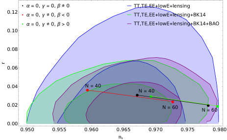
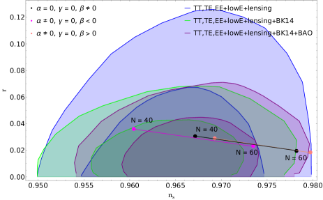
Figure 1: (Color online) Constraints on $n_{s}$ and $r$ from CMB measurements of different potential. PLANCK alone, PLANCK+BK15, PLANCK+BK15+BAO upto $68\%$ Confidence Level.

In Figure 1, we have plotted the contour plot in the $n_{s}$–r plane for different values of $\alpha$, $\beta$, and $\gamma$, respectively. To see the effect of the non-minimally coupled term i.e. the $RT$ mixing term, first, we switch off the other two terms (by fixing $\alpha=0$ and $\gamma=0$). The blue, green, and purple regions show the contours of recent Planck 2018 in $n_{S}-r$ plane. The red line indicates the plot corresponding to the non-zero $\beta$ value for $N=40$ and $60$. We have shown the effect of a fixed value of positive and negative $\beta$ for two cases (i) $\alpha=0$ and $\gamma\neq 0$ (ii) $\alpha\neq 0$ and $\gamma=0$. The left-hand side of Figure 1 shows the effect for $\beta<0$ while the right-hand side of the same figure represents the effect for the $\beta>0$ case. The black line in the plot represents the case where $\alpha\neq 0$, $\gamma=0$ and $\beta<0$ while the blue line represents the case where $\alpha=0$, $\gamma\neq 0$. All three cases match suitably well with the Planck 2018 data as far as the left-hand side of the plot. The right-hand side of the plot is shown for the positive $\beta$ value. We also see the same two cases (i) $\alpha=0$ and $\gamma\neq 0$ (ii) $\alpha\neq 0$ and $\gamma=0$ for $\beta>0$. Here the green line indicates the case when $\alpha\neq 0$ and $\gamma=0$ while the purple line indicates $\alpha=0$ and $\gamma\neq 0$ case. We can see that as $\beta>0$, the scalar spectral index value shifts towards the $+3\sigma$ value of $n_{s}$ while for the $\beta<0$ case, the $n_{s}$ value is within $\pm 3\sigma$ range. Both cases match well with the Planck 2018 $n_{s}-r$ predictions.

3.2 Model II: $V=V_{0}\bigl{(}\frac{\lambda\phi^{p}}{1+\lambda\phi^{p}}\bigr{)}$: Results and Analysis

Next, we consider the fractional potential for inflationary expansion,

$$V=V_{0}\frac{\lambda\phi^{p}}{1+\lambda\phi^{p}}$$ (33)

where $V_{0}$ is a constant, $p$ and $\lambda$ are the potential parameters. In our analysis, we have taken the potential parameters $p=2$, and $\lambda=1,2$, respectively. With $p=2$, the fractional potential was first studied by Eshagli et al.[44]. This potential have also been studied in the minimal scenario in normal Einstein gravity and non-minimal coupled gravity[15].
The modified potential slow-roll parameters for this potential are found to be

$$\epsilon_{\tilde{V}}=\frac{1}{2\Bigl{\{}\bigl{(}1+\alpha\bigr{)}\bigl{(}1+\gamma\bigr{)}+\frac{4\beta\lambda V_{0}\phi^{p}}{1+\lambda\phi^{p}}\Bigr{\}}}\times\Biggl{[}\frac{p\bigl{(}1+\alpha-\frac{4\beta\lambda V_{0}\phi^{p}}{1+\lambda\phi^{p}}\bigr{)}}{\phi\bigl{(}1+\lambda\phi^{p}\bigr{)}}\Biggr{]}^{2}$$ (34)

$$\begin{split}\eta_{\tilde{V}}&=-\frac{1}{\phi^{2}(1+\lambda\phi^{p})^{3}\Bigl{\{}1+\gamma+\lambda\phi^{p}+4V_{0}\beta\lambda\phi^{p}+\gamma\lambda\phi^{p}+\alpha\bigl{(}1+\gamma\bigr{)}\bigl{(}1+\lambda\phi^{p}\bigr{)}\Bigr{\}}^{2}}\Biggl{[}p~{}\Bigl{\{}1+\alpha+\alpha\lambda\phi^{p}-\\ &\qquad\bigl{(}-1+4V_{0}\beta\bigr{)}\lambda\phi^{p}\Bigr{\}}\times\biggl{[}\bigl{(}1+\lambda\phi^{p}\bigr{)}\Bigl{\{}1+\alpha+\alpha\lambda\phi^{p}-\bigl{(}-1+4V_{0}\beta\bigr{)}\lambda\phi^{p}\Bigr{\}}\Bigl{\{}1+\gamma+\lambda\phi^{p}+4V_{0}\beta\lambda\phi^{p}\\ &\qquad+\gamma\lambda\phi^{p}+\alpha\bigl{(}1+\gamma\bigr{)}\bigl{(}1+\lambda\phi^{p}\bigr{)}\Bigr{\}}+p\biggl{\{}-1-\lambda\phi^{p}-2V_{0}\beta\lambda\phi^{p}+\lambda^{2}\phi^{2p}-2V_{0}\beta\lambda^{2}\phi^{2p}-8V_{0}^{2}\beta^{2}\lambda^{2}\phi^{2p}\\ &\qquad+\lambda^{3}\phi^{3p}-16V_{0}^{2}\beta^{2}\lambda^{3}\phi^{3p}+\bigl{(}1+\gamma\bigr{)}\bigl{(}-1+\lambda\phi^{p}\bigr{)}\bigl{(}\alpha+\alpha\lambda\phi^{p}\bigr{)}^{2}-\gamma\bigl{(}1+\lambda\phi^{p}\bigr{)}\Bigl{\{}1+\bigl{(}-1+4V_{0}\beta\bigr{)}\lambda^{2}\\ &\qquad\times\phi^{2p}\Bigr{\}}-2\alpha\bigl{(}1+\lambda\phi^{p}\bigr{)}\Bigl{\{}1+V_{0}\beta\lambda\phi^{p}-\lambda^{2}\phi^{2p}+\gamma\bigl{\{}1+(-1+2V_{0}\beta)\lambda^{2}\phi^{2p}\bigr{\}}\Bigr{\}}\biggr{\}}\biggr{]}\Biggr{]}\\ \end{split}$$ (35)

The scalar spectral index and tensor to scalar ratio can be obtained as,

$$\begin{split}n_{s}&=1-\frac{3}{\Bigl{\{}\bigl{(}1+\alpha\bigr{)}\bigl{(}1+\gamma\bigr{)}+\frac{4\beta\lambda V_{0}\phi^{p}}{1+\lambda\phi^{p}}\Bigr{\}}}\times\Biggl{[}\frac{p\bigl{(}1+\alpha-\frac{4\beta\lambda V_{0}\phi^{p}}{1+\lambda\phi^{p}}\bigr{)}}{\phi\bigl{(}1+\lambda\phi^{p}\bigr{)}}\Biggr{]}^{2}-\frac{2}{\phi^{2}(1+\lambda\phi^{p})^{3}}\times\\ &\qquad\frac{1}{\Bigl{\{}1+\gamma+\lambda\phi^{p}+4V_{0}\beta\lambda\phi^{p}+\gamma\lambda\phi^{p}+\alpha\bigl{(}1+\gamma\bigr{)}\bigl{(}1+\lambda\phi^{p}\bigr{)}\Bigr{\}}^{2}}\Biggl{[}p~{}\Bigl{\{}1+\alpha+\alpha\lambda\phi^{p}-\bigl{(}-1+4V_{0}\beta\bigr{)}\lambda\phi^{p}\Bigr{\}}\\ &\qquad\times\biggl{[}\bigl{(}1+\lambda\phi^{p}\bigr{)}\Bigl{\{}1+\alpha+\alpha\lambda\phi^{p}-\bigl{(}-1+4V_{0}\beta\bigr{)}\lambda\phi^{p}\Bigr{\}}\Bigl{\{}1+\gamma+\lambda\phi^{p}+4V_{0}\beta\lambda\phi^{p}+\gamma\lambda\phi^{p}+\alpha\bigl{(}1+\gamma\bigr{)}\times\\ &\qquad\bigl{(}1+\lambda\phi^{p}\bigr{)}\Bigr{\}}+p\biggl{\{}-1-\lambda\phi^{p}-2V_{0}\beta\lambda\phi^{p}+\lambda^{2}\phi^{2p}-2V_{0}\beta\lambda^{2}\phi^{2p}-8V_{0}^{2}\beta^{2}\lambda^{2}\phi^{2p}+\lambda^{3}\phi^{3p}-16V_{0}^{2}\beta^{2}\lambda^{3}\\ &\qquad\times\phi^{3p}+\bigl{(}1+\gamma\bigr{)}\bigl{(}-1+\lambda\phi^{p}\bigr{)}\bigl{(}\alpha+\alpha\lambda\phi^{p}\bigr{)}^{2}-\gamma\bigl{(}1+\lambda\phi^{p}\bigr{)}\Bigl{\{}1+\bigl{(}-1+4V_{0}\beta\bigr{)}\lambda^{2}\phi^{2p}\Bigr{\}}-2\alpha\bigl{(}1+\lambda\phi^{p}\bigr{)}\\ &\qquad\times\Bigl{\{}1+V_{0}\beta\lambda\phi^{p}-\lambda^{2}\phi^{2p}+\gamma\bigl{\{}1+(-1+2V_{0}\beta)\lambda^{2}\phi^{2p}\bigr{\}}\Bigr{\}}\biggr{\}}\biggr{]}\Biggr{]}\\ \end{split}$$ (36)

$$r=\frac{8}{\Bigl{\{}\bigl{(}1+\alpha\bigr{)}\bigl{(}1+\gamma\bigr{)}+\frac{4\beta\lambda V_{0}\phi^{p}}{1+\lambda\phi^{p}}\Bigr{\}}}\times\Biggl{[}\frac{p\bigl{(}1+\alpha-\frac{4\beta\lambda V_{0}\phi^{p}}{1+\lambda\phi^{p}}\bigr{)}}{\phi\bigl{(}1+\lambda\phi^{p}\bigr{)}}\Biggr{]}^{2}$$ (37)

For potential $V=V_{0}\bigl{(}\frac{\lambda\phi^{p}}{1+\lambda\phi^{p}}\bigr{)}$,	$\alpha=0$,	$\gamma=0$,	$p=2$
Range of $\beta$	$\lambda$	$\beta$	$\phi$	$\phi_{f}$	N	$n_{s}$	r
$-0.04<\beta<0.0171$	1	-0.01	4.5	0.845504	54	0.969229	0.00392
$-0.07<\beta<-0.008$	2	-0.04	4.0	0.752338	59	0.964436	0.00290
When $\alpha=0$,	$\gamma\neq 0$,	$p=2$
Range of $\gamma$	$\lambda$	$\gamma$	$\beta$	$\phi$	$\phi_{f}$	N	$n_{s}$	r
$-0.55<\gamma<-0.25$	1	-0.4	0.01	5	0.938257	54	0.973615	0.00274
$-0.58<\gamma<-0.4$	1	-0.48	-0.05	6	1.10431	58	0.960944	0.00285
$-0.05<\gamma<0.5$	2	0.25	0.01	3.5	0.65924	52	0.97281	0.00288
$-0.1<\gamma<0.35$	2	-0.09	-0.05	4	0.785847	50	0.955188	0.00366
When $\gamma=0$,	$\alpha\neq 0$,	$p=2$
Range of $\alpha$	$\lambda$	$\alpha$	$\beta$	$\phi$	$\phi_{f}$	N	$n_{s}$	r
$-0.03<\alpha<0.2$	1	0.05	0.05	4	0.794314	41	0.974207	0.00415
$0.2<\alpha<1.0$	1	0.8	-0.001	5	0.974634	47	0.966983	0.00343
$0.25<\alpha<0.7$	2	0.48	0.05	3.8	0.728853	43	0.972846	0.00246
$-0.43<\alpha<0.15$	2	-0.08	-0.001	3.5	0.693562	44	0.964678	0.00374

Table 2: For $V=V_{0}\bigl{(}\frac{\lambda\phi^{p}}{1+\lambda\phi^{p}}\bigr{)}$, the e-fold number $N$ and the spectral index parameters $n_{s}$ and $r$ calculated for a fixed value of $\phi$ and $\alpha$ are presented. Here $\phi$ is rescaled as $\frac{\phi}{M_{Pl}}$.

We have tabulated our results in Table (2) for different choices of the potential parameters. With the $RT$ mixing term only, and for $\beta=-0.01(-0.04)$, $\lambda=1(2)$ and setting $\alpha=\gamma=0$, we find the e-fold parameter $N=54(59)$ , the spectral index $n_{s}=0.969229(0.964436)$ and the tensor-to-scalar ratio $r=0.00392(0.0029)$, while by taking $\alpha=0$ and $\gamma=-0.3338(0.1087)$ and $\beta=-0.010(0.001)$, we find $N=47(46)$ and $n_{s}=0.96497(0.97333)$ and $r=0.05178(0.024805)$. We observe that the value of $n_{s}$ and $r$ for fixed $\alpha$, $\gamma$, and a range of $\beta$ ($-0.04<\beta<0.0171$) matches well with the data provided by WMAP and Planck 2018. By including $T$ term along with $RT$ mixing term, we have seen that $\gamma$ lies between $[-0.55,-0.25],[0.05,0.5]$ for $\beta>0$ and $[-0.58,-0.4],[-0.1,0.35]$ for $\beta<0$ corresponding to $\lambda=1,2$. The range of $\alpha$ we have got by taking $\gamma=0$ as $[-0.03,0.2],[0.25,0.7]$ for $\beta>0$ and $[0.2,1.0],[-0.43,0.15]$ for $\beta<0$ corresponding to $\lambda=1,2$.

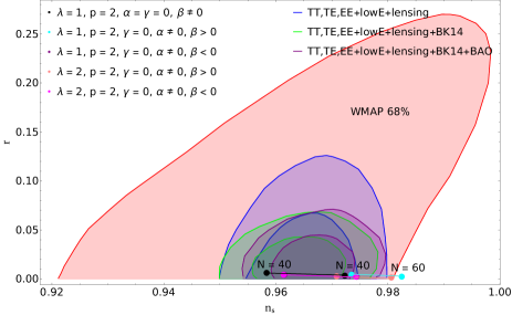
Figure 2: (Color online) Constraints on $n_{s}$ and $r$ from CMB measurements of different potential. Shaded regions are allowed by WMAP measuremnts, PLANCK alone, PLANCK+BK15, PLANCK+BK15+BAO upto $68\%$ Confidence Level.

Figure 2 represents the contour plot of $n_{s}$–$r$ for different values of $\alpha$, $\beta$, $\gamma$ and the potential parameters ($\lambda$ and p) for the fractional potential $V=V_{0}\frac{\lambda\phi^{p}}{1+\lambda\phi^{p}}$. Red contour represents the WMAP $n_{s}-r$ data with $68\%$ C.L. while the blue, purple and green regions represent the Planck 2018 data. Next, we have taken two different values of the potential parameter $\lambda=1$, $2$, and for fixed $p=2$. Then, considered different cases for fixed $\beta$ value (for both cases $\beta>0$ and $\beta<0$) for two cases: (i) $\alpha=0$ and $\gamma\neq 0$ (ii) $\alpha\neq 0$ and $\gamma=0$. In the left-hand side plot of Figure 2, first, we have shown how the $n_{s}~{}-~{}r$ values deviate for non-zero $\beta$ value as we fix $\alpha=\gamma=0$. The black line indicates the plot corresponding to the non-zero $\beta$ value for $N=40$ and $60$. The yellow and blue lines are overlapped for $\beta>0$ case where we have taken the parameter values as $\lambda=1$, $p=2$, $\alpha=0$, $\gamma\neq 0$ and $\lambda=2$, $p=2$, $\alpha=0$, $\gamma\neq 0$, respectively with $N=40$ and $60$. The identical overlapping scenario for $N=40$ and $60$ can be seen for the $\beta<0$ case where we have taken the parameter values as $\lambda=1$, $p=2$, $\alpha=0$, $\gamma\neq 0$ and $\lambda=2$, $p=2$, $\alpha=0$, $\gamma\neq 0$, respectively. On the right-hand side of Figure 2, we have shown the same black line for the non-zero $\beta$ value for both $\alpha=\gamma=0$ where p is fixed and $\lambda=1$. Then we have considered two different cases as before $\alpha\neq 0$, $\gamma=0$ when $\beta>0$ and $\beta<0$. In this case, unlike the previous case, we can see that for different $\lambda$’s, distinct lines are coming for $N=40$ and $60$. The blue line and purple line are for the case when $\lambda=1$, $p=2$, $\gamma=0$, $\alpha\neq 0$, $\beta>0$ and $\lambda=1$, $p=2$, $\gamma=0$, $\alpha\neq 0$, $\beta<0$, respectively. The orange and pink lines are for the case when $\lambda=2$ for $\beta>0$ and $\beta<0$, respectively. We can see from the plot that as we switch on the parameter $\alpha$ and $\beta<0$, the $n_{s}$ value shifts towards the $+3\sigma$ while for the negative $\beta$, the $n_{s}$ value shifts beyond $+3\sigma$ value. It is important to note that the $n_{s}$ - r curves cross the boundary of the dark blue contour i.e. falls in the WMAP data range.

4 Conclusion

In this manuscript, we have investigated, in detail, a family of non-minimally coupled gravity theories slow-roll inflationary models. In the theory, non-minimal curvature-inflaton couplings result from the assumption that the trace of the energy-momentum tensor $T$ seen in the gravitational action corresponds to inflaton. In the present work, we have studied modified $f(R,T)$ gravity with $f(R,T)=R\bigl{(}1+\alpha+\kappa^{4}\beta T\bigr{)}+\kappa^{2}\gamma T$. In particularly, we have focused on the impact of the mixing term $RT$ on inflationary cosmology. In the literature, several $f(R,T)$ models are taken into consideration, where the impacts of $R$ and $T$ are viewed individually. The $RT$ mixing term introduces non-minimal derivative couplings, and higher-order derivative terms can be seen in the equation of motion. By assuming that the inflaton rolls so slowly on its potential that we can neglect the higher-order derivative terms, which makes it quite plausible to write it in Einstein’s frame.
We have considered two different types of slow-roll inflaton potentials, e.g., $V=V_{0}\left(1+\ln{\phi}\right)$ and $V=V_{0}\frac{\lambda\phi^{p}}{1+\lambda\phi^{p}}$, have derived the modified slow-roll parameters and different cosmological parameters for these potentials. First, we considered the impact of $RT$ mixing term only by taking $\alpha=\gamma=0$, and later on, we investigated each term by including them one by one together with the $RT$ mixing term. We can observe that although the tensor-to-scalar ratio $r$ value for both the potentials agrees with observational data along with e-fold number $N$ lies between $40-60$, the scalar spactral index $n_{s}$ value matches with the PLANCK 2018 data for logarithmic potential whereas $n_{s}$ lies in WMAP region for another potential at least for $N=60$. We get $n_{s}$ beyond $3\sigma$ region of PLANCK 2018 data by turning off all the modified gravity parameters (i.e. $\alpha=\beta=\gamma=0$) in order to have $N=40-70$ which motivates us towards modified gravity. From Table (2), we see that the e-fold $50<N<60$ after including $RT$ mixing term along with $T$ term.
We can compare our result with Ref.[39] where the result without $RT$ mixing term is shown for $V=V_{0}\frac{\lambda\phi^{p}}{1+\lambda\phi^{p}}$. Ref. [14] have found the e-fold number $N\approx 31$(a slightly lower value) and the spectral index $n_{s}\approx 0.99$ for Einstein gravity in the case of Logarithmic inflaton potential, whereas our results presented in Table 1 shows that those are consistent with the observational values of $n_{s}$ and the desired e-fold number $N$. This validates our analysis (with the $RT$ mixing term ) on the estimation of several modified gravity and potential parameters in light of the CMBR observational data.

References

- [1] A. Einstein, The Berlin Years: Writings, 1914-1917 , 6, 117,1915
- [2] A. H. Guth, Phys. Rev. D,23 (1981) 347–356.
- [3] E. Kolb, M. S. Turner The Early Universe,(CNC Press), 1994.
- [4] A. Liddle, An Introduction to Modern Cosmology, Willey Publication, (2003).
- [5] D. N. Spergel et al., Physical Review Letter, 92, 20, (2004).
- [6] F. G. Smoot, AIP Conference Proceedings CONF-981098, AIP 476, 1, (1999).
- [7] P. AR. Ade, The Astrophysical Journal, 792, 62, (2014).
- [8] Y. Akrami, Astronomy & Astrophysics, 641, 61, (2020).
- [9] G. Hinsaw, Astrophysical Journal Supplement Series, 208, 19, (2013).
- [10] A. D. Linde, Phys. Lett. B108, 389-393, (1982).
- [11] A. D. Linde, Phys. Lett. B129, 177-181, (1983).
- [12] D. Baumann, TASI lecture on Inflation, arXiv:0907.5424v2 [hep-th].
- [13] W. H. Kinney, TASI lecture on Inflation, arXiv:0902.1529v2 [astro-ph].
- [14] Ø. Grøn, Universe, 4, 15, (2018).
- [15] P. Sarkar, Ashmita, P. K. Das, arXiv:2205.05532v2.
- [16] K. Nozari and S. D. Sadatian, Mod. Phys. Lett., A23, (2008).
- [17] D. Y. Cheong, S. M. Lee, S. C. Park JCAP, 2022, 029, (2022).
- [18] Y. Jin and S. Tsujikawa, Classical and Quantum Gravity, 23, 353 (2006)
- [19] K. i. Maeda, Class. Quantum Gravity 3, 233, (1986).
- [20] F.S. Accetta, D.J. Zoller, M.S. Turner, Phys. Rev. D 31, 3046 (1985).
- [21] V. Faraoni, Phys. Rev. D 53 (1996),6813 [astro-ph/9602111].
- [22] V. Faraoni, Phys. Rev. D 62 (2000),023504 [gr-qc/0002091].
- [23] V. Dzhunushaliev, V. Folomeev, B. Kleihaus and J. Kunz, Eur. Phys. J. C 74 (2014), 2743 [1312.0225]
- [24] V. Dzhunushaliev, V. Folomeev, B. Kleihaus and J. Kunz, Eur. Phys. J. C 75 (2015) 157 [1501.00886].
- [25] R.V. Lobato, G.A. Carvalho, A.G. Martins and P.H.R.S. Moraes, Eur. Phys. J. Plus 134 (2019) 132 [1803.08630].
- [26] C.-Y. Chen and Y.-H. Kung, Phys. Dark Univ. 35 (2022) 100956 [2108.04853].
- [27] L. Parker, Phys. Rev. Lett. 21, 562 (2014)
- [28] L. Parker, Phys. Rev. D 3, 2546 (1971).
- [29] T. Harko, F.S.N. Lobo, S. Nojiri and S.D. Odintsov, Phys. Rev. D 84 (2011) 024020 [1104.2669].
- [30] M. Roshan and F. Shojai, Phys. Rev. D 94 (2016) 044002 [1607.06049].
- [31] O. Bertolami, C.G. Boehmer, T. Harko and F.S.N. Lobo, Phys. Rev. D 75 (2007) 104016 [0704.1733].
- [32] Y. Bisabr, 2012 arxiv:1205.0328v2 [gr-qc]
- [33] P.H.R.S. Moraes, P.K Sahoo, Eur. Phys. J. C 77, 480 (2017)
- [34] S. Nojiri and S.D. Odintsov, Phys. Lett. B 599 (2004) 137 [astro-ph/0403622].
- [35] G. Allemandi, A. Borowiec, M. Francaviglia and S.D. Odintsov, Phys. Rev. D 72 (2005) 063505 [gr-qc/0504057].
- [36] Che-Yu Chen, Y. Reyimuaji, X. Zhang, Phys of Dark Unv. 38 (2022), 101130
- [37] X. Zhang, Che-Yu Chen, Y. Reyimuaji, Physical Review D,105, 4, (2022), [arXiv: 2108.07546]
- [38] N. Godani, International Journal of Geometric Methods in Modern Physics, 16, 02, (2018).
- [39] Ashmita, P.Sarkar, P. K. Das, IJMPD, 2250120 (2022) 1-14
- [40] Ashmita, P. Sarkar, P. K. Das, arXiv:2210.07788
- [41] D. H. Lyth, A. Riotto, Phys. Rep., bf 314, 1999, 1–146.
- [42] R. Y. Guo,X. Zhang,Eur. Phys. J. C,77 2017, 882.
- [43] A. Hebecker, S. C. Kraus, D. Lüst, D, S. Steinfurt, T. Weigand,Nucl. Phys. B, 854 2012, 509–551.
- [44] M. Eshagli, M. Zarei, N. Riazi, A. Kiasatpour, J. Cosmol. Astropart. Phys., 2015, 037, [arXiv:1505.03556].