Recursive Identification of Set-Valued Systems
under Uniform Persistent Excitations

Abstract

This paper studies the control-oriented identification problem of set-valued moving average systems with uniform persistent excitations and observation noises. A stochastic approximation-based (SA-based) algorithm without projections or truncations is proposed. The algorithm overcomes the limitations of the existing empirical measurement method and the recursive projection method, where the former requires periodic inputs, and the latter requires projections to restrict the search region in a compact set. To analyze the convergence property of the algorithm, the distribution tail of the estimation error is proved to be exponentially convergent through an auxiliary stochastic process. Based on this key technique, the SA-based algorithm appears to be the first to reach the almost sure convergence rate of $O(\sqrt{\ln\ln k/k})$ theoretically in the non-periodic input case. Meanwhile, the mean square convergence is proved to have a rate of $O(1/k)$, which is the best one even under accurate observations. A numerical example is given to demonstrate the effectiveness of the proposed algorithm and theoretical results.

Set-valued systems, stochastic systems, recursive identification, stochastic approximation, uniform persistent excitations.

1 Introduction

Set-valued systems emerge widely in practical fields. For example, in automotive and chemical process applications, oxygen sensors are widely used for evaluating gas oxygen contents [1, 2, 3]. Inexpensive oxygen sensors are switching types that change their voltage outputs sharply when excess oxygen in the gas is detected. More examples can be seen in genetic association studies [5, 4], radar target recognition [6], and credit scoring [7], etc. The appearance of the above set-valued sensors brings forward new requirements for identification and control theory. As a result, the research of set-valued systems has received much attention in the past two decades despite the difficulty that set-valued observations can only supply very limited information. For example, identification problems have been widely researched for such systems since [2]. Adaptive control laws and consensus protocols of set-valued multi-agent systems have also been developed based on identification methods with periodic inputs or projection algorithms [8, 9, 10, 11]. However, there are still limitations on existing control-oriented identification methods. Under this background, we continue the development along the direction of seeking more general control-oriented identification methods for set-valued systems.

There are some excellent identification algorithms proposed for set-valued systems [12, 13, 14, 15, 16, 17], many of which are offline. Offline methods take full advantage of the statistical property of the set-valued outputs, and require fewer assumptions than the online ones. However, recursive forms of the corresponding offline methods are difficult to be constructed and analyzed. And, the computational complexity increases geometrically when offline identification methods are applied to system controls. Therefore, control-oriented identification methods are required to be online.

Moreover, the control-oriented identification methods are supposed to keep a freedom for the input design. Many efficient online identification methods require strict conditions for inputs. For example, [18, 19] propose stochastic approximation algorithms with expanding truncations for set-valued systems. [20] identifies the parameters with a stochastic gradient based estimation method. Strong consistency is obtained for all these algorithms, but the strong consistency relies on independent and identically distributed (i.i.d.) inputs, which seems not suitable to design control laws. Besides, the empirical measurement method for set-valued systems is proved to be strongly convergent and achieves Cramér-Rao lower bounds asymptotically [21, 22, 23, 24, 25, 26, 27, 2, 28]. However, the effectiveness analysis of the empirical measurement method is based on periodic input signals, which causes that the corresponding adaptive control laws waste a lot of information [8, 10, 11].

Identification algorithms with potential in effective control design have been proposed for set-valued output systems [29, 30, 31, 9, 32, 33], but there are still limitations in these works. The identification method proposed in [29, 30] relies on designable quantizers. However, most physical sensors that produce set-valued signals are undesignable and even time-invariant. In the time-invariant quantizer case, [31, 9, 32, 33] raise recursive projection algorithms, which rely on projections to restrict the search region in a compact set. The construction of projections require a priori information about the approximate location of the unknown parameters. Besides, the projections bring nonnegligible extra computation cost especially to the quasi-Newton type recursive projection algorithm [32]. Therefore, a new online control-oriented identification method without projections or truncations should be considered.

The main difficulty lies in the trade-off between little information that one set-valued measurement contains and the features of online algorithms. On the one hand, a single observation only contains binary information, hence the identification of set-valued systems requires the accumulation of a number of output signals. On the other hand, when we update online algorithms, only the present or recent several signals can be used. As a result, it is difficult to reveal how the accumulation of the set-valued signals affects the trend of the online algorithm.

To overcome the difficulty, the paper constructs an SA-based algorithm for the set-valued moving average (MA) system identification problem under uniform persistent excitations. Different from recursive projection algorithms [31, 9, 32, 33], the SA-based algorithm does not rely on projections or truncations. Instead, the effectiveness analysis of the algorithm relies on a stochastic process with averaged observations (SPAO). By using the new methodology, the SA-based algorithm achieves a better almost sure convergence rate under weaker assumptions compared with recursive projection algorithms. Besides, without projections, the SA-based algorithm can be applied in more control problems.

The main contributions of the paper are as follows.

1. A new SA-based identification algorithm without projections is proposed for set-valued MA systems with uniform persistent excitations. For comparison, the SA-based algorithm neither relies on periodic inputs in contrast with the set-valued system identification algorithms in [21, 22, 23, 24, 25, 26, 27, 2, 28], nor relies on projections or truncations in contrast with the algorithms in [29, 30, 31, 9, 32, 33].

2. The convergence properties of the SA-based identification algorithm are established. To be specific, the almost sure convergence and mean square convergence are induced through the exponential convergence of the estimation error distribution tail. Besides, the almost sure convergence rate is proved to reach $O(\sqrt{\ln\ln k/k})$, which is firstly achieved among online identification algorithms of stochastic set-valued systems under non-periodic inputs. Moreover, the mean square convergence rate is proved to reach $O(1/k)$, which is the best mean square convergence rate in theory under set-valued observations and even accurate ones.

3. A new constructive methodology is developed for the convergence analysis of set-valued system identification algorithms. Specially, an auxiliary stochastic process named SPAO is constructed to reveal the connection between the accumulation of the set-valued signals and the convergence properties of the algorithm. Moreover, the methodology is also shown to be practical for a common class of recursive identification algorithms of set-valued systems.

The rest of the paper is organized as follows. Section 2 formulates the identification problem. Section 3 constructs an SA-based identification algorithm of set-valued systems. The convergence analysis is given in Section 4. Section 4.1 constructs an auxiliary stochastic process named SPAO and discusses its property. Based on SPAO, Section 4.2 estimates the distribution tail of the estimation error, and gives the almost sure and mean square convergence. Almost sure and mean square convergence rates are estimated in Section 4.3 and Section 4.4, respectively. A numerical example is simulated in Section 5 to demonstrate the theoretical results. Concluding remarks and future works are given in Section 6.

Notation

In the rest of the paper, $\mathbb{R}$ and $\mathbb{R}^{n}$ are the sets of real numbers and $n$-dimensional real vectors, respectively. $I_{\{\cdot\}}$ denotes the indicator function, whose value is 1 if its argument (a formula) is true, and 0, otherwise. $\|x\|=\|x\|_{2}$ is the Euclidean norm for vector $x$. $I_{n}$ is an $n\times n$ identity matrix. $\lfloor x\rfloor$ is the largest integer that is smaller than or equal to $x\in\mathbb{R}$. The positive part of $x$ is denoted as $x^{+}=\max\{x,0\}$. For square matrices $A_{l},\ldots,A_{k}$, denote $\prod_{i=l}^{k}A_{i}=A_{k}\cdots A_{l}$ for $k\geq l$ and $\prod_{i=k+1}^{k}A_{i}=I_{n}$. Relations between two series $a_{k}$ and $b_{k}$ are defined as

1. $a_{k}=O(b_{k})$ if $a_{k}=c_{k}b_{k}$ for an ultimately bounded $c_{k}$ as $k$ goes to $\infty$;

2. $a_{k}=o(b_{k})$ if $a_{k}=c_{k}b_{k}$ for a $c_{k}$ that converges to $0$ as $k$ goes to $\infty$.

2 Problem formulation

Consider the MA system:

$$y_{k}=\phi_{k}^{\top}\theta+d_{k},\quad k\geq 1,$$ (1)

where $\phi_{k}=\phi(u_{k},u_{k-1},\ldots,u_{k-\bar{n}+1})\in\mathbb{R}^{n}$ is a regressed function of inputs $u_{k}$ for some $\bar{n}>0$, $\theta\in\mathbb{R}^{n}$ is the unknown parameter, and $d_{k}$ is the system noise, respectively. The unobserved system output $y_{k}$ is measured by a binary-valued sensor with a fixed threshold $C$, which can be represented by an indicator function

$$s_{k}=I_{\{y_{k}\leq C\}}=\begin{cases}1,\quad y_{k}\leq C;\\ 0,\quad y_{k}>C.\\ \end{cases}$$ (2)

Our goal is to identify the unknown parameter $\theta$ based on the regressed vector $\phi_{k}$ and the binary observation $s_{k}$.

Assumption 1.

The sequence $\{\phi_{k},k\geq 1\}$ is uniformly bounded, i.e.,

$$\sup\limits_{k\geq 1}\left\|\phi_{k}\right\|\leq M<\infty,$$

and there exist a positive integer $N\geq n$ and a real number $\delta>0$ such that

$$\frac{1}{N}\sum^{k+N-1}_{i=k}\phi_{i}\phi_{i}^{\top}\geq\delta I_{n},k\geq 1.$$ (3)

Remark 1.

The condition (3) is usually called “uniform persistent excitation condition” or “sufficiently rich condition” [34, 31]. Assumption 1 is a common condition in the identification field. For example, it is adopted in recursive projection algorithms [31, 9]. Moreover, Assumption 1 is also required for the identification methods in [34] when the observations are accurate and deterministic.

Assumption 2.

The system noise $\{d_{k},k\geq 1\}$ is a sequence of i.i.d. random variables with zero mean and finite covariance $\sigma^{2}$, whose distribution and density function are denoted as $F(\cdot)$ and $f(\cdot)$, respectively. The distribution $F(\cdot)$ is Lipschitz continuous, and the density function $f(\cdot)$ satisfies

$$\inf\limits_{x\in\mathfrak{X}}f(x)>0$$ (4)

for any bounded open set $\mathfrak{X}$.

For simplicity of notation, denote

$$F_{k}=F\left(C-\phi_{k}^{\top}\theta\right),\quad f_{k}=f\left(C-\phi_{k}^{\top}\theta\right).$$

Then $\mathbb{E}s_{k}=\mathbb{P}\{y_{k}\leq C\}=F_{k}$.

Remark 2.

Gaussian noise, Laplacian noise and $t$-distribution noise are all examples satisfying Assumption 2. Moreover, if (4) does not hold for the system noise, we can add a dither to the binary sensor [2]. Under Assumption 2, the density function $f(\cdot)$ is bounded because of the Lipschitz continuity of the distribution function $F(\cdot)$.

3 Identification algorithm

In this section, we will give an SA-based algorithm for the MA system (1) with binary observation (2).

The realization of the SA-based algorithm is inspired by a new viewpoint for the system. Note that $F_{k}$ contains the entire information of $\phi_{k}^{\top}\theta$. Hence, we treat $F_{k}$ as an accurate but nonlinear output. The rest of the observation, i.e., $s_{k}-F_{k}$, is treated as an independent noise. Under Assumptions 1 and 2, $\hat{\theta}=\theta$ if and only if

$$\sum_{i=k}^{k+N-1}\phi_{i}^{\top}(\theta-\hat{\theta})\left(F\left(C-\phi_{i}^{\top}\hat{\theta}\right)-F_{i}\right)=0.$$

Then, the SA-based algorithm is designed as

$$\hat{\theta}_{k}= \hat{\theta}_{k-1}+\rho_{k}\phi_{k}\left(F\left(C-\phi_{k}^{\top}\hat{\theta}_{k-1}\right)-F_{k}\right)$$

$$+\rho_{k}\phi_{k}\left(F_{k}-s_{k}\right)$$

$$= \hat{\theta}_{k-1}+\rho_{k}\phi_{k}\left(F\left(C-\phi_{k}^{\top}\hat{\theta}_{k-1}\right)-s_{k}\right),$$

where $\rho_{k}$ is the step size satisfying $\sum_{i=1}^{\infty}\rho_{i}=\infty$ and $\sum_{i=1}^{\infty}\rho^{2}_{i}<\infty$.

Denote

$$\hat{F}_{k}=F\left(C-\phi_{k}^{\top}\hat{\theta}_{k-1}\right).$$

Set $\rho_{k}=\beta/k$, where $\beta>0$ is a constant coefficient. Then, the SA-based algorithm is given as follows.

$$\hat{\theta}_{k}=\hat{\theta}_{k-1}+\frac{\beta\phi_{k}}{k}\left(\hat{F}_{k}-s_{k}\right).$$ (5)

The observation error $\hat{\theta}_{k}-\theta$ is denoted as $\tilde{\theta}_{k}$.

Remark 3.

In addition to $\rho_{k}=\beta/k$, other types of step sizes can be applied to the SA-based algorithm. For example, $\rho_{k}=\beta_{k}/(1+\sum_{i=1}^{k}\left\|\phi_{i}\right\|^{2})$ for $0<\underline{\beta}\leq\beta_{k}\leq\overline{\beta}<\infty$ is an alternative step size. Besides, in Algorithm (5), $\hat{F}_{k}$ is used to approximate $s_{k}$ because $\hat{F}_{k}=\mathbb{E}[s_{k}(\theta)|\theta=\hat{\theta}_{k-1}]$. Therefore, in the multiple threshold case with threshold number $q$, Algorithm (5) also works after replacing $\hat{F}_{k}$ with $\mathbb{E}[s_{k}^{q}(\theta)|\theta=\hat{\theta}_{k-1}]$, where $s_{k}^{q}$ is the corresponding observation in $\{0,1,\ldots,q\}$.

4 Convergence

This section will focus on the convergence analysis of the algorithm including the distribution tail, almost sure convergence rate and mean square convergence rate. An auxiliary stochastic process is introduced firstly to assist in the analysis.

4.1 Stochastic process with averaged observations (SPAO)

In this subsection, we will introduce an auxiliary stochastic process satisfying

1. the trajectory of the stochastic process gradually approaches that of the estimation error $\tilde{\theta}_{k}$;

2. the convergence property of the stochastic process is easy to analyze compared with that of the algorithm.

The construction is inspired by the idea that $\beta\phi_{k}(F_{k}-s_{k})$ can be replaced by the linear combination of $T_{k}$ and $T_{k-1}$, where

$$T_{k}=\frac{\sum_{i=1}^{k}\beta\phi_{i}(F_{i}-s_{i})}{k},$$ (6)

i.e.,

$$\beta\phi_{k}(F_{k}-s_{k})= \sum_{i=1}^{k}\beta\phi_{i}(F_{i}-s_{i})-\sum_{i=1}^{k-1}\beta\phi_{i}(F_{i}-s_{i})$$

$$= k\left(T_{k}-T_{k-1}\right)+T_{k-1}.$$

Define $\psi_{k}=\tilde{\theta}_{k}-T_{k}$. Then, by the transformation above,

$$\psi_{k}= \psi_{k-1}+\frac{\beta\phi_{k}}{k}\left(F\left(C-\phi_{k}^{\top}\theta-\phi_{k}^{\top}\psi_{k-1}-\phi_{k}^{\top}T_{k-1}\right)\right.$$

$$\qquad\qquad\left.-F\left(C-\phi_{k}^{\top}\theta\right)\right)+\frac{T_{k-1}}{k}.$$ (7)

The above stochastic process is named as SPAO. With SPAO, the convergence property of the algorithm can be analyzed through that of $T_{k}$.

Remark 4.

For general stochastic approximation methods, $T_{k}$ is also used to verify the robustness of the algorithm (cf. [35], Assumption 2.7.3 and Theorem 2.7.1).

To analyze the properties of SPAO $\psi_{k}$, we should firstly estimate the distribution tail of $T_{k}$.

Lemma 1.

Let $T_{k}$ be defined in (6), and assume that

1. $\phi_{k}\in\mathbb{R}^{n}$ is bounded;

2. $s_{k}\in\{0,1\}$ is an independent binary random variable with expectation $F_{k}$;

3. $\sup_{k}F_{k}<1$ and $\inf_{k}F_{k}>0$.

Then, for any $\varepsilon\in(0,\frac{1}{2})$ , there exists $m>0$ such that

$$\mathbb{P}\left\{\sup_{j\geq k}j^{\varepsilon}\left\|T_{j}\right\|>1\right\}=O\left(\exp(-mk^{1-2\varepsilon})\right).$$

The proof is given in Section 7.1.

Next, we give the following lemma to describe the distance between $\psi_{k}$ and the estimation error $\tilde{\theta}_{k}$ in three different senses based on Lemma 1.

Lemma 2.

Assume that

1. System (1) with binary observation (2) satisfies Assumptions 1 and 2;

2. $T_{k}$ is defined in (6), and $\psi_{k}=\tilde{\theta}_{k}-T_{k}$.

Then, we have

1. for any $\varepsilon\in(0,\frac{1}{2})$, there exists $m>0$ such that $\mathbb{P}\left\{\lVert\tilde{\theta}_{k}-\psi_{k}\rVert>k^{-\varepsilon}\right\}=O\left(\exp\left(-mk^{1-2\varepsilon}\right)\right)$;

2. $\lVert\tilde{\theta}_{k}-\psi_{k}\rVert=O\left(\sqrt{\ln\ln k/k}\right)$, a.s.;

3. $\mathbb{E}\lVert\tilde{\theta}_{k}-\psi_{k}\rVert^{2}=O(1/k)$.

Proof.

Since $\tilde{\theta}_{k}-\psi_{k}=T_{k}$, the three parts of the lemma can be obtained immediately from Lemma 1, the law of the iterated logarithm ([36], Theorem 10.2.1) and $\mathbb{E}\left\|T_{k}\right\|^{2}=O(1/k)$, respectively. ∎

Then, by using Lemmas 1 and 2, the following theorem estimates the distribution tail of SPAO $\psi_{k}$.

Theorem 1.

Under the conditions of Lemma 2, for any $M^{\prime}>0$ and $\varepsilon\in(0,\frac{1}{2})$, when $k$ is sufficiently large,

$$\left\{\lVert\psi_{k}\rVert^{2}<M^{\prime}\right\}\supseteq\left\{\sup_{j\geq\lfloor k^{1-\varepsilon}\rfloor}j^{\varepsilon}\left\|T_{j}\right\|\leq 1\right\}.$$

Furthermore, there exists $m>0$ such that

$$\mathbb{P}\left\{\lVert\psi_{k}\rVert^{2}\geq M^{\prime}\right\}=O\left(\exp(-mk^{(1-\varepsilon)(1-2\varepsilon)})\right).$$

Proof.

Set $k_{s}=\lfloor k^{1-\varepsilon}\rfloor$ and $k_{s}^{\prime}=k-N\lfloor\frac{k-k_{s}}{N}\rfloor$. It is worth mentioning that $k_{s}^{\prime}\in[k_{s},k_{s}+N-1]$, and $k-k_{s}^{\prime}$ is divisible by $N$. Assume that $\sup_{j\geq k_{s}}j^{\varepsilon}\left\|T_{j}\right\|\leq 1$ is true in the rest of the proof. Then, it suffices to prove that $\left\|\psi_{k}\right\|^{2}<M^{\prime}$.

We firstly simplify the recursive formula of $\left\|\psi_{k}\right\|^{2}$. By (4.1) and the monotonicity and Lipschitz continuity of $F(\cdot)$, for any positive real number $b$, we have

$$\left\|\psi_{k}\right\|^{2}$$

$$\leq \left\|\psi_{k-1}\right\|^{2}\!+\frac{2\beta\phi_{k}^{\top}\psi_{k-1}}{k}\!\left(F(C\!-\phi_{k}^{\top}\theta-\phi_{k}^{\top}T_{k-1}-\phi_{k}^{\top}\psi_{k-1})\right.$$

$$\left.-F(C-\phi_{k}^{\top}\theta)\right)+\frac{2\psi_{k-1}^{\top}T_{k-1}}{k}+\frac{\left(\beta\lVert\phi_{k}\rVert+\lVert T_{k-1}\rVert\right)^{2}}{k^{2}}$$

$$= \left\|\psi_{k-1}\right\|^{2}\!+\frac{2\beta\phi_{k}^{\top}\psi_{k-1}}{k}\!\left(F(C\!-\phi_{k}^{\top}\theta-\phi_{k}^{\top}T_{k-1}-\phi_{k}^{\top}\psi_{k-1})\right.$$

$$\qquad\qquad\left.-F(C-\phi_{k}^{\top}\theta-\phi_{k}^{\top}T_{k-1})\right)+O\left(k^{-1-\varepsilon/2}\right)$$

$$\leq \left\|\psi_{k-1}\right\|^{2}+\frac{2\beta\phi_{k}^{\top}\psi_{k-1}}{k}\left(F(C-\phi_{k}^{\top}\theta-\phi_{k}^{\top}T_{k-1}-b)\right.$$

$$\qquad\qquad\left.-F(C-\phi_{k}^{\top}\theta-\phi_{k}^{\top}T_{k-1})\right)I_{\{\phi_{k}^{\top}\psi_{k-1}\geq b\}}$$

$$+\frac{2\beta\phi_{k}^{\top}\psi_{k-1}}{k}\left(F(C-\phi_{k}^{\top}\theta-\phi_{k}^{\top}T_{k-1}+b)\right.$$

$$\qquad\qquad\left.-F(C-\phi_{k}^{\top}\theta-\phi_{k}^{\top}T_{k-1})\right)I_{\{\phi_{k}^{\top}\psi_{k-1}\leq-b\}}$$

$$+O\left(k^{-1-\varepsilon/2}\right).$$ (8)

By Assumption 2 and the boundedness of $C-\phi_{k}^{\top}\theta-\phi_{k}^{\top}T_{k-1}$, there exists $B>0$ such that

$$-2\beta \left(F(C-\phi_{k}^{\top}\theta-\phi_{k}^{\top}T_{k-1}-b)\right.$$

$$\qquad\qquad\left.-F(C-\phi_{k}^{\top}\theta-\phi_{k}^{\top}T_{k-1})\right)>B,$$

$$2\beta \left(F(C-\phi_{k}^{\top}\theta-\phi_{k}^{\top}T_{k-1}+b)\right.$$

$$\qquad\qquad\left.-F(C-\phi_{k}^{\top}\theta-\phi_{k}^{\top}T_{k-1})\right)>B,$$

which together with (4.1) implies

$$\left\|\psi_{k}\right\|^{2}\!\leq\left\|\psi_{k-1}\right\|^{2}-\frac{B\lvert\phi_{k}^{\top}\psi_{k-1}\rvert}{k}I_{\{\lvert\phi_{k}^{\top}\psi_{k-1}\rvert\geq b\}}+O\!\left(k^{-1-\varepsilon/2}\right)\!.$$

Set $b=\frac{\sqrt{\delta}M^{\prime}}{2\sqrt{2}}$. Then, by Lemma 4, there exists $k^{\prime}\in[k+1,k+N]$ such that

$$\left\|\psi_{k+N}\right\|^{2}$$

$$\leq \left\|\psi_{k}\right\|^{2}-\sum_{i=k+1}^{k+N}\frac{B\lvert\phi_{i}^{\top}\psi_{i-1}\rvert}{i}I_{\left\{\lvert\phi_{i}^{\top}\psi_{i-1}\rvert\geq\frac{\sqrt{\delta}M^{\prime}}{2\sqrt{2}}\right\}}$$

$$+\sum_{i=k+1}^{k+N}O\left(i^{-1-\varepsilon/2}\right)$$

$$\leq \left\|\psi_{k}\right\|^{2}-\frac{B\lvert\phi_{k^{\prime}}^{\top}\psi_{k^{\prime}-1}\rvert}{k+N}I_{\left\{\lvert\phi_{k^{\prime}}^{\top}\psi_{k^{\prime}-1}\rvert\geq\frac{\sqrt{\delta}M^{\prime}}{2\sqrt{2}}\right\}}+O\left(k^{-1-\varepsilon/2}\right)$$

$$\leq \left\|\psi_{k}\right\|^{2}-\frac{B\sqrt{\delta}}{\sqrt{2}}\frac{\left\|\psi_{k}\right\|}{k+N}I_{\left\{\left\|\psi_{k}\right\|\geq\frac{M^{\prime}}{2}\right\}}+O\left(k^{-1-\varepsilon/2}\right).$$

Hence, when $k=k_{s}^{\prime}+N(t-1)$, we have

$$\left\|\psi_{k_{s}^{\prime}+Nt}\right\|^{2}$$

$$\leq \left\|\psi_{k_{s}^{\prime}+N(t-1)}\right\|^{2}-\frac{B\sqrt{\delta}}{\sqrt{2}}\frac{\left\|\psi_{k_{s}^{\prime}+N(t-1)}\right\|}{k_{s}^{\prime}+Nt}I_{\left\{\lVert\psi_{k_{s}^{\prime}+Nt}\rVert\geq\frac{M^{\prime}}{2}\right\}}$$

$$+O\left((k_{s}^{\prime}+Nt)^{-1-\varepsilon/2}\right).$$ (9)

Since $\lim\limits_{k\to\infty}k_{s}^{\prime}=\infty$, we have

$$\lim\limits_{k\to\infty}\sum_{t=1}^{\infty}(k_{s}^{\prime}+Nt)^{-1-\varepsilon/2}=0.$$

Then, by (4.1) and Lemma 5, when $k$ is sufficiently large, we have

$$\left\|\psi_{k}\right\|^{2}=\left\|\psi_{k_{s}^{\prime}+N\lfloor\frac{k-\lfloor k^{1-\varepsilon}\rfloor}{N}\rfloor}\right\|^{2}<\max\left\{M^{\prime},\Delta_{k}^{2}+\frac{M^{\prime}}{2}\right\},$$

where

$$\Delta_{k}=\left(\left\|\psi_{k_{s}^{\prime}}\right\|-\frac{B\sqrt{\delta}}{2\sqrt{2}N}\ln\left(\frac{\lfloor\frac{k-\lfloor k^{1-\varepsilon}\rfloor}{N}\rfloor+\frac{k_{s}^{\prime}}{N}+1}{\frac{k_{s}^{\prime}}{N}+1}\right)\right)^{+}.$$

Note that $\ln\left(\frac{\lfloor(k-\lfloor k^{1-\varepsilon}\rfloor)/N\rfloor+k_{s}^{\prime}/N+1}{k_{s}^{\prime}/N+1}\right)$ is of the same order as $\ln k$ since $k_{s}^{\prime}=O(k^{1-\varepsilon})$. And, by Corollary 6.2, $\psi_{k_{s}^{\prime}}=O\left(\sqrt{\ln k}\right)$. Therefore, when $k$ is sufficiently large, $\Delta_{k}=0$ and $\left\|\psi_{k}\right\|^{2}<M^{\prime}$, which proves the theorem. ∎

Remark 5.

The distribution tail estimation of SPAO $\psi_{k}$ in Theorem 1 can be promoted as in Theorem 7 (cf. Section 7.2).

Remark 6.

It is worth noting that the constructed SPAO can not only be adapted to the SA-based algorithm, but also can be extended to a class of identification algorithms of the set-valued systems. The details are given in Section 8.

4.2 Estimate of the distribution tail

In this subsection, the distribution tail of the estimation error will be estimated.

Theorem 2.

If System (1) with binary observations (2) satisfies Assumptions 1 and 2, then for any $M^{\prime}>0$ and $\varepsilon>0$, there exists $m>0$ such that

$$\mathbb{P}\left\{\sup\limits_{j\geq k}\lVert\tilde{\theta}_{j}\rVert^{2}\geq M^{\prime}\right\}=O\left(\exp(-mk^{1-\varepsilon})\right).$$

Proof.

Reminding that $\tilde{\theta}_{k}=\psi_{k}+T_{k}$, by Theorem 1, for sufficiently large $k$, we have

$$\left\{\sup_{j\geq\lfloor k^{1-\varepsilon}\rfloor}j^{\varepsilon}\left\|T_{j}\right\|\leq 1\right\}$$

$$\subseteq \left\{\lVert\psi_{k}\rVert^{2}<\frac{M^{\prime}}{4}\right\}\cap\left\{\lVert T_{k}\rVert^{2}\leq\frac{M^{\prime}}{4}\right\}\subseteq\left\{\lVert\tilde{\theta}_{k}\rVert^{2}<M^{\prime}\right\},$$

and hence,

$$\left\{\sup\limits_{j\geq k}\lVert\tilde{\theta}_{j}\rVert^{2}\geq M^{\prime}\right\}\subseteq \bigcup_{j\geq k}\left\{\sup_{j_{0}\geq\lfloor j^{1-\varepsilon}\rfloor}j_{0}^{\varepsilon}\left\|T_{j_{0}}\right\|>1\right\}$$

$$= \left\{\sup_{j\geq\lfloor k^{1-\varepsilon}\rfloor}j^{\varepsilon}\left\|T_{j}\right\|>1\right\}.$$

So, by Lemma 1,

$$\mathbb{P}\{\sup_{j\geq k}\lVert\tilde{\theta}_{j}\rVert^{2}\geq M^{\prime}\}=O\left(\exp(-mk^{(1-\varepsilon)(1-2\varepsilon)})\right).$$

Thus, the theorem can be proved by the arbitrariness of $\varepsilon$. ∎

Remark 7.

Theorem 2 estimates the distribution tail of the estimation error $\tilde{\theta}_{k}$. For the convergence analysis of identification algorithms, the existing works are usually interested in the asymptotic properties of the estimation error distribution. For example, the asymptotic normality of $\rho_{k}^{-1/2}\tilde{\theta}_{k}$ is given for general stochastic approximation algorithms under different conditions (cf. [35], Section 3.3 and [37]). For the set-valued system with i.i.d. inputs and designable quantizer, [20] also analyzes the asymptotic normality of the algorithm. Compared with the asymptotic normality, Theorem 2 weakens the description of the estimate distribution in the neighborhood of $\theta$, but gives a better description on the exponential tail of the estimation error. This helps to obtain the almost sure and mean square convergence of the algorithm.

Theorem 3.

Under the conditions of Theorem 2, Algorithm (5) converges to $\theta$ in both almost sure and mean square sense.

Proof.

The almost sure convergence can be immediately obtained by Theorem 2.

By Theorems 2 and 6.1, for any $M^{\prime}>0$ and $\varepsilon>0$, there exists $m>0$ such that

$$\mathbb{E}\lVert\tilde{\theta}_{k}\rVert^{2}= \int_{\{\lVert\tilde{\theta}_{k}^{2}\rVert<M^{\prime}\}}\lVert\tilde{\theta}_{k}\rVert^{2}\text{d}\mathbb{P}+\int_{\{\lVert\tilde{\theta}_{k}^{2}\rVert\geq M^{\prime}\}}\lVert\tilde{\theta}_{k}\rVert^{2}\text{d}\mathbb{P}$$

$$< M^{\prime}+O\left(\ln k\cdot\exp(-mk^{1-\varepsilon})\right)=M^{\prime}+o(1).$$

Thus, the mean square convergence can be obtained by the arbitrariness of $M^{\prime}$. ∎

Remark 8.

When the inputs are periodic, the mean square convergence of the empirical measurement method without truncation is also proved by the estimation of the distribution tail [11]. The distribution tail is relatively easy to be obtained for the empirical measurement method, because there is a direct connection between the average of the set-valued observations and the distribution tail. But, in the SA-based algorithm, the connection is obscure. Therefore, SPAO is needed to reveal the connection.

4.3 Almost sure convergence rate

In this subsection we will estimate the almost sure convergence rate of the SA-based algorithm.

Before the analysis, we define

$$\underline{f}(x)=\lim\limits_{z\to(M\left\|\theta\right\|+x)^{+}}\inf\limits_{t\in[C-z,C+z]}f(t)>0,\quad\forall x\geq 0,$$ (10)

and

$$\underline{f}=\underline{f}(0).$$ (11)

The convergence rate of the algorithm depends on $\underline{f}$.

Remark 9.

Under Assumption 1, $\underline{f}$ is the lower bound of $f(C-\phi_{k}^{\top}\theta)$ for all possible regressors $\phi_{k}$, which motivates us to analyze $\underline{f}(\cdot)$ and $\underline{f}$. By (10), we give properties of $\underline{f}(\cdot)$ and $\underline{f}$.

1. $\underline{f}(\cdot)$ is monotonically decreasing and right continuous.

2. $\lim\limits_{x\to 0}\underline{f}(x)=\underline{f}$ and $\lim\limits_{x\to\infty}\underline{f}(x)=0$. Then, by Theorem 1,

   $$\lim\limits_{k\to\infty}\underline{f}\left(\left|\phi_{k}^{\top}\psi_{k-1}\right|\right)=\underline{f},\quad\text{a.s.}$$

3. The following inequality holds for $\underline{f}(\cdot)$.

   $$\underline{f}(x)\leq\inf\limits_{t\in[C-M\left\|\theta\right\|-x,C+M\left\|\theta\right\|+x]}f(t),$$

   $$\underline{f}\leq\inf_{t\in[C-M\left\|\theta\right\|,C+M\left\|\theta\right\|]}f(t).$$

   The equality is achieved when $\underline{f}(\cdot)$ is continuous.

4. If $f(\cdot)$ is locally Lipschitz continuous, so is $\underline{f}(\cdot)$.

The almost sure convergence rate of the algorithm can be achieved through that of $\psi_{k}$.

Theorem 4.

Under the conditions of Lemma 2, for any $\varepsilon>0$, we have

$$\psi_{k}=\begin{cases}O\left(\sqrt{\frac{\ln\ln k}{k}}\right),&\eta>\frac{1}{2};\\ O\left(\frac{1}{k^{\eta-\varepsilon}}\right),&\eta\leq\frac{1}{2},\end{cases}\quad\text{a.s.,}$$ (12)

where $\eta=\beta\delta\underline{f}$ with $\underline{f}$ defined in (11). If $f(\cdot)$ is assumed to be locally Lipschitz continuous, then the almost sure convergence rate can be promoted into

$$\psi_{k}=\begin{cases}O\left(\sqrt{\frac{\ln\ln k}{k}}\right),&\eta>\frac{1}{2};\\ O\left(\ln k\sqrt{\frac{\ln\ln k}{k}}\right),&\eta=\frac{1}{2};\\ O\left(\frac{1}{k^{\eta}}\right),&\eta<\frac{1}{2}.\end{cases}\quad\text{a.s.}$$ (13)

Proof.

The proof is based on Lemma 7.

For the proof of (12), we firstly simplify the recursive formula of $\left\|\psi_{k}\right\|$. In (4.1), by the Lagrange mean value theorem ([38], Theorem 5.3.1), there exists $\xi_{k}$ between $C-\phi_{k}^{\top}\theta-\phi_{k}^{\top}\psi_{k-1}$ and $C-\phi_{k}^{\top}\theta$ such that

$$F(C-\phi_{k}^{\top}\theta-\phi_{k}^{\top}T_{k-1}-\phi_{k}^{\top}\psi_{k-1})-F(C-\phi_{k}^{\top}\theta)$$

$$= f(\xi_{k})\phi_{k}^{\top}\psi_{k-1}+O\left(T_{k-1}\right).$$ (14)

Then, by the law of the iterated logarithm ([36], Theorem 10. 2.1),

$$F(C-\phi_{k}^{\top}\theta-\phi_{k}^{\top}T_{k-1}-\phi_{k}^{\top}\psi_{k-1})-F_{k}$$

$$= f(\xi_{k})\phi_{k}^{\top}\psi_{k-1}+O\left(\sqrt{\frac{\ln\ln k}{k}}\right),\ \text{a.s.},$$

which together with (4.1) implies

$$\psi_{k}=\left(I_{n}-\frac{\beta f(\xi_{k})}{k}\phi_{k}\phi_{k}^{\top}\right)\psi_{k-1}+O\left(\sqrt{\frac{\ln\ln k}{k^{3}}}\right),\quad\text{a.s.}$$

Note that except for the first few steps, we have

$$\left\|\prod_{i=k-N+1}^{k}\left(I_{n}-\frac{\beta f(\xi_{i})}{i}\phi_{i}\phi_{i}^{\top}\right)\right\|$$

$$\leq \left\|I_{n}-\frac{\beta}{k}\sum_{i=k-N+1}^{k}f(\xi_{i})\phi_{i}\phi_{i}^{\top}\right\|+O\left(\frac{1}{k^{2}}\right)$$

$$\leq \left\|I_{n}-\frac{\beta}{k}\underline{f}\left(\max\limits_{k-N<i\leq k}\!\left|\phi_{i}^{\top}\psi_{i-1}\right|\right)\!\sum_{i=k-N+1}^{k}\!\!\!\phi_{i}\phi_{i}^{\top}\right\|+O\left(\frac{1}{k^{2}}\right)$$

$$\leq \left(1-\frac{\beta\delta N}{k}\underline{f}\left(\max\limits_{k-N<i\leq k}\left|\phi_{i}^{\top}\psi_{i-1}\right|\right)\right)+O\left(\frac{1}{k^{2}}\right),$$ (15)

where $\underline{f}(\cdot)$ is defined in (10). Denote

$$\underline{f}_{k|N}=\underline{f}\left(\max\limits_{k-N<i\leq k}\left|\phi_{i}^{\top}\psi_{i-1}\right|\right).$$

Then, we have

$$\left\|\psi_{k}\right\|\leq\left(1-\frac{\beta\delta N}{k}\underline{f}_{k|N}\right)\left\|\psi_{k-N}\right\|+O\left(\sqrt{\frac{\ln\ln k}{k^{3}}}\right),\quad\text{a.s.}$$ (16)

By Item (b) of Remark 9, $\lim\limits_{k\to\infty}\underline{f}_{k|N}=\underline{f}$ almost surely. Therefore, for any $\varepsilon\in(0,\beta\delta\underline{f})$, there almost surely exists a $k_{a}$ such that for all $k\geq k_{a}$, we have $\beta\delta\underline{f}_{k|N}>\beta\delta\underline{f}-\varepsilon$, and thus, by (16),

$$\left\|\psi_{k}\right\|\leq\left(1-\frac{N}{k}(\eta-\varepsilon)\right)\left\|\psi_{k-N}\right\|+O\left(\sqrt{\frac{\ln\ln k}{k^{3}}}\right),\quad\text{a.s.}$$

Without loss of generality, assume that $k-k_{a}$ is divisible by $N$. Then, by Lemma 7, one can get

$$\left\|\psi_{k}\right\|$$

$$\leq \prod_{i=1}^{\frac{k-k_{a}}{N}}\left(1-\frac{N(\eta-\varepsilon)}{k_{a}+iN}\right)\left\|\psi_{k_{a}}\right\|$$

$$+O\left(\sum_{l=1}^{\frac{k-k_{a}}{N}}\prod_{i=l+1}^{\frac{k-k_{a}}{N}}\left(1-\frac{N(\eta-\varepsilon)}{k_{a}+iN}\right)\sqrt{\frac{\ln\ln(k_{a}+lN)}{(k_{a}+lN)^{3}}}\right)$$

$$= O\left(\frac{1}{k^{\eta-\varepsilon}}\right)$$

$$+O\left(\sum_{l=1}^{\frac{k-k_{a}}{N}}\prod_{i=l+1}^{\frac{k-k_{a}}{N}}\left(1-\frac{N(\eta-\varepsilon)}{k_{a}+iN}\right)\sqrt{\frac{\ln\ln(l+2)}{l^{3}}}\right)$$

$$= \begin{cases}O\left(\sqrt{\frac{\ln\ln k}{k}}\right),&\eta-\varepsilon>\frac{1}{2};\\ O\left(\ln k\sqrt{\frac{\ln\ln k}{k}}\right),&\eta-\varepsilon=\frac{1}{2};\\ O\left(\frac{1}{k^{\eta-\varepsilon}}\right),&\eta-\varepsilon<\frac{1}{2}.\end{cases}\quad\text{a.s.}$$

Notice that $\varepsilon$ can be arbitrarily chosen, which implies that when $\eta>1/2$, we can choose $\varepsilon>0$ such that $\eta-\varepsilon>1/2$. Hence, (12) is proved.

Then, we prove (13). For sufficiently large $k$,

$$1-\frac{\beta\delta N}{k}\underline{f}_{k|N}\leq\left(1+\frac{\beta\delta N}{k}\left(\underline{f}-\underline{f}_{k|N}\right)\right)\left(1-\frac{\beta\delta N}{k}\underline{f}\right).$$ (17)

which together with (16) implies

$$\left.\left\|\psi_{k}\right\|\middle/\prod_{i=N+1}^{k}\left(1+\frac{\beta\delta N}{i}\left(\underline{f}-\underline{f}_{i|N}\right)\right)\right.$$

$$\leq \left(1-\frac{N\eta}{k}\right)\left.\left\|\psi_{k-N}\right\|\middle/\prod_{i=N+1}^{k-N}\left(1+\frac{\beta\delta N}{i}\left(\underline{f}-\underline{f}_{i|N}\right)\right)\right.$$

$$+O\left(\sqrt{\frac{\ln\ln k}{k^{3}}}\right),\quad\text{a.s.}$$ (18)

By (12) and Item (d) of Remark 9, $\underline{f}-\underline{f}_{i|N}$ converges to $0$ at a polynomial rate. Hence, we have

$$\prod_{i=N+1}^{\infty}\left(1+\frac{\beta\delta N}{i}\left(\underline{f}-\underline{f}_{i|N}\right)\right)<\infty$$

Then, (13) can be proved by (4.3) and Lemma 7. ∎

Then, the almost sure convergence rate of the algorithm can be obtained by Theorem 4.

Theorem 5.

Under the conditions of Theorem 2, for any $\varepsilon>0$,

$$\tilde{\theta}_{k}=\begin{cases}O\left(\sqrt{\frac{\ln\ln k}{k}}\right),&\eta>\frac{1}{2};\\ O\left(\frac{1}{k^{\eta-\varepsilon}}\right),&\eta\leq\frac{1}{2}.\end{cases}\quad\text{a.s,}$$

where $\eta=\beta\delta\underline{f}$ with $\underline{f}$ defined in (11). If the density function $f(\cdot)$ is assumed to be locally Lipschitz continuous, then the almost sure convergence rate can be promoted into

$$\tilde{\theta}_{k}=\begin{cases}O\left(\sqrt{\frac{\ln\ln k}{k}}\right),&\eta>\frac{1}{2};\\ O\left(\ln k\sqrt{\frac{\ln\ln k}{k}}\right),&\eta=\frac{1}{2};\\ O\left(\frac{1}{k^{\eta}}\right),&\eta<\frac{1}{2}.\end{cases}\quad\text{a.s.}$$

Proof.

The theorem can be obtained by Lemmas 2 and 4. ∎

Remark 10.

By Theorem 5, the algorithm may not achieve the optimal almost sure convergence rate when the coefficient $\eta$ is smaller than $1/2$. Since $\eta=\beta\delta\underline{f}$, the convergence rate of the algorithm depends on the step size, the inputs, the noise distribution and the relationship between the threshold $C$ and $M\left\|\theta\right\|$. However, $M\left\|\theta\right\|$ relies on the true parameter $\theta$. Thus, the almost sure convergence rate of Algorithm (5) cannot be known without priori information on $\theta$. The problem can be solved if the step size is designed as $\rho_{k}=\beta_{k}/k$, where

$$\beta_{k}>\left.1\middle/\left(2\delta\lim\limits_{z\to(M\lVert\hat{\theta}_{k}\rVert)^{+}}\inf\limits_{t\in[C-z,C+z]}f(t)\right)\right..$$

The analysis for the modified algorithm is consistent with the algorithm with time-invariant $\beta$.

Remark 11.

For the identification problem of stochastic set-valued systems, $O(\sqrt{\ln\ln k/k})$ is the best almost sure convergence rate. In the periodic input case, the empirical measurement algorithm in [2] generates a maximum likelihood estimate (cf. [14], Lemma 4). The almost sure convergence rate of the empirical measurement algorithm is $O(\sqrt{\ln\ln k/k})$ [23]. In the non-periodic input case, Theorem 5 appears to be the first to achieve the almost sure convergence rate of $O(\sqrt{\ln\ln k/k})$ theoretically. [31] achieves the almost sure convergence rate of $O(\sqrt{\ln k/k})$ for the recursive projection method. And, the almost sure convergence rate of stochastic approximation algorithms with expanding truncations is $O(1/k^{\varepsilon})$ for $\varepsilon\in(0,1/2)$ [19]. When properly selecting $\beta$, the almost sure convergence rate of Algorithm (5) is better than both of them.

4.4 Mean square convergence rate

This subsection will estimate the mean square convergence rate of the SA-based algorithm.

Theorem 6.

Under the conditions of Theorem 2, for any $\varepsilon>0$,

$$\mathbb{E}\lVert\tilde{\theta}_{k}\rVert^{2}=\begin{cases}O\left(\frac{1}{k}\right),&\eta>\frac{1}{2};\\ O\left(\frac{1}{k^{2\eta-\varepsilon}}\right),&\eta\leq\frac{1}{2},\end{cases}$$ (19)

where $\eta=\beta\delta\underline{f}$ with $\underline{f}$ defined in (11). If $f(\cdot)$ is assumed to be locally Lipschitz continuous, then the mean square convergence rate can be promoted into

$$\mathbb{E}\lVert\tilde{\theta}_{k}\rVert^{2}=\begin{cases}O\left(\frac{1}{k}\right),&\eta>\frac{1}{2};\\ O\left(\frac{\ln k}{k}\right),&\eta=\frac{1}{2};\\ O\left(\frac{1}{k^{2\eta}}\right),&\eta<\frac{1}{2}.\end{cases}$$ (20)

Proof.

To prove (19), we firstly simplify the recursive formula of $\mathbb{E}\lVert\tilde{\theta}_{k}\rVert^{2}$.

By (5) and the Lagrange mean value theorem (​ [38], Theorem 5.3.1) , there exists $\zeta_{k}$ between $C-\phi_{k}^{\top}\theta$ and $C-\phi_{k}^{\top}\theta-\phi_{k}^{\top}\tilde{\theta}_{k-1}$ such that

$$\tilde{\theta}_{k}= \tilde{\theta}_{k-1}+\frac{\beta\phi_{k}}{k}\left(\hat{F}_{k}-F_{k}\right)+\frac{\beta\phi_{k}}{k}\left(F_{k}-s_{k}\right)$$

$$= \left(I_{n}-\frac{\beta}{k}f(\zeta_{k})\phi_{k}\phi_{k}^{\top}\right)\tilde{\theta}_{k-1}+\frac{\beta\phi_{k}}{k}\left(F_{k}-s_{k}\right)$$

$$= \prod_{i=k-N+1}^{k}\left(I_{n}-\frac{\beta}{i}f(\zeta_{i})\phi_{i}\phi_{i}^{\top}\right)\tilde{\theta}_{k-N}$$

$$+\sum_{l=k-N+1}^{k}\prod_{i=l+1}^{k}\left(I_{n}-\frac{\beta}{i}f(\zeta_{i})\phi_{i}\phi_{i}^{\top}\right)\frac{\beta\phi_{l}}{l}\left(F_{l}-s_{l}\right)$$

$$= \prod_{i=k-N+1}^{k}\left(I_{n}-\frac{\beta}{i}f(\zeta_{i})\phi_{i}\phi_{i}^{\top}\right)\tilde{\theta}_{k-N}$$

$$+\sum_{l=k-N+1}^{k}\frac{\beta\phi_{l}}{l}\left(F_{l}-s_{l}\right)+O\left(\frac{1}{k^{2}}\right).$$

Similar to (4.3), except for the first few steps, we have

$$\left\|\prod_{i=k-N+1}^{k}\left(I_{n}-\frac{\beta f(\zeta_{i})}{i}\phi_{i}\phi_{i}^{\top}\right)\right\|\leq\left(1-\underline{f}_{k|N}^{\prime}\right)+O\left(\frac{1}{k^{2}}\right),$$

where $\underline{f}_{k|N}^{\prime}=\frac{\beta\delta N}{k}\underline{f}\left(\max\limits_{k-N<i\leq k}\left|\phi_{i}^{\top}\tilde{\theta}_{i-1}\right|\right)$, and $\underline{f}(\cdot)$ is defined in (10). Besides, noticing that $\tilde{\theta}_{k-N}$ is independent of $\sum_{l=N+1}^{k}\frac{\beta\phi_{l}}{l}\left(F_{l}-s_{l}\right)$, we have

$$\mathbb{E}\left[\left(\sum_{l=k-N+1}^{k}\frac{\beta\phi_{l}}{l}\left(F_{l}-s_{l}\right)\right)^{\top}\right.$$

$$\qquad\left.\cdot\prod_{i=k-N+1}^{k}\left(I_{n}-\frac{\beta}{i}f(\zeta_{i})\phi_{i}\phi_{i}^{\top}\right)\tilde{\theta}_{k-N}\right]$$

$$= \mathbb{E}\left[\left(\sum_{l=k-N+1}^{k}\frac{\beta\phi_{l}}{l}\left(F_{l}-s_{l}\right)\right)^{\top}\right.$$

$$\qquad\left.\cdot\left(\prod_{i=k-N+1}^{k}\left(I_{n}-\frac{\beta}{i}f(\zeta_{i})\phi_{i}\phi_{i}^{\top}\right)-I_{n}\right)\tilde{\theta}_{k-N}\right]$$

$$= O\left(\frac{1}{k^{2}}\right).$$

Therefore, for sufficiently large $k$, one can get

$$\mathbb{E}\lVert\tilde{\theta}_{k}\rVert^{2}\leq\mathbb{E}\left[\left(1-\frac{\beta\delta N}{k}\underline{f}_{k|N}^{\prime}\right)^{2}\lVert\tilde{\theta}_{k-N}\rVert^{2}\right]+O\left(\frac{1}{k^{2}}\right).$$ (21)

By Theorem 2 and the property of $\underline{f}(\cdot)$, $\mathbb{P}\{\underline{f}_{k|N}^{\prime}<\underline{f}-\frac{\varepsilon}{2\beta\delta}\}=O(\exp(-mk^{1/2}))$. Hence, by Corollary 6.1, we have

$$\mathbb{E}\left[\left(1-\frac{\beta\delta N}{k}\underline{f}_{k|N}^{\prime}\right)^{2}\lVert\tilde{\theta}_{k-N}\rVert^{2}\right]$$

$$\leq \int_{\left\{\underline{f}_{k|N}^{\prime}\geq\underline{f}-\frac{\varepsilon}{2\beta\delta}\right\}}\left(1-\frac{N}{k}\left(\eta-\frac{\varepsilon}{2}\right)\right)^{2}\lVert\tilde{\theta}_{k-N}\rVert^{2}\text{d}\mathbb{P}$$

$$+\int_{\left\{\underline{f}_{k|N}^{\prime}<\underline{f}-\frac{\varepsilon}{2\beta\delta}\right\}}\lVert\tilde{\theta}_{k-N}\rVert^{2}\text{d}\mathbb{P}$$

$$= \left(1-\frac{N}{k}\left(\eta-\frac{\varepsilon}{2}\right)\right)^{2}\mathbb{E}\lVert\tilde{\theta}_{k-N}\rVert^{2}$$

$$+O\left(\ln k\cdot\exp(-mk^{1/2})\right).$$

Substituting the above estimate into (21) gives

$$\mathbb{E}\lVert\tilde{\theta}_{k}\rVert^{2}\leq\left(1-\frac{N}{k}\left(\eta-\frac{\varepsilon}{2}\right)\right)^{2}\mathbb{E}\lVert\tilde{\theta}_{k-N}\rVert^{2}+O\left(\frac{1}{k^{2}}\right).$$

Thus, (19) can be proved by Lemma 7.

Then, we prove (20). Similar to (17), for sufficiently large $k$,

$$1-\frac{\beta\delta N}{k}\underline{f}_{k|N}^{\prime}\leq\left(1+\frac{\beta\delta N}{k}\left(\underline{f}-\underline{f}_{k|N}^{\prime}\right)\right)\left(1-\frac{\beta\delta N}{k}\underline{f}\right).$$

Therefore, by (21) and $\eta=\beta\delta\underline{f}$, one can get

$$\mathbb{E}\lVert\tilde{\theta}_{k}\rVert^{2}\leq \left(1-\frac{N\eta}{k}\right)^{2}\mathbb{E}\left[\left(1+\frac{\beta\delta N}{k}\left(\underline{f}-\underline{f}_{k|N}^{\prime}\right)\right)^{2}\right.$$

$$\qquad\qquad\left.\cdot\lVert\tilde{\theta}_{k-N}\rVert^{2}\right]+O\left(\frac{1}{k^{2}}\right).$$ (22)

By Item (d) of Remark 9, since $f(\cdot)$ is assumed to be locally Lipschitz continuous here, $\underline{f}(\cdot)$ is also locally Lipschitz continuous. Hence, if $\lVert\tilde{\theta}_{j}\rVert\leq j^{-\varepsilon^{\prime}}$ for a $\varepsilon^{\prime}>0$ and all $j=k-N+1,\ldots,k$, then there exists $L>0$ such that $\underline{f}-\underline{f}_{k|N}^{\prime}\leq Lk^{-\varepsilon^{\prime}}$, which together with Corollaries 6.1 and 7.1 implies that there exist positive numbers $m$ and $\varepsilon$ such that

$$\mathbb{E}\left[\left(1+\frac{\beta\delta N}{k}\left(\underline{f}-\underline{f}_{k|N}^{\prime}\right)\right)^{2}\lVert\tilde{\theta}_{k-N}\rVert^{2}\right]$$

$$\leq \left(1+\frac{\beta\delta NL}{k^{1+\varepsilon^{\prime}}}\right)^{2}\int_{\cap_{j=k-N+1}^{k}\{\lVert\tilde{\theta}_{j}\rVert\leq j^{-\varepsilon^{\prime}}\}}\lVert\tilde{\theta}_{k-N}\rVert^{2}\text{d}\mathbb{P}$$

$$+O\left(\ln k\cdot\exp(-mk^{1-\varepsilon})\right)$$

$$\leq \left(1+\frac{\beta\delta NL}{k^{1+\varepsilon^{\prime}}}\right)^{2}\mathbb{E}\lVert\tilde{\theta}_{k-N}\rVert^{2}\text{d}\mathbb{P}+O\left(\ln k\cdot\exp(-mk^{1-\varepsilon})\right).$$

Substituting the above estimate into (4.4) gives

$$\mathbb{E}\lVert\tilde{\theta}_{k}\rVert^{2}\!\leq\!\left(1-\frac{N\eta}{k}\right)^{2}\!\left(1+\frac{\beta\delta NL}{k^{1+\varepsilon^{\prime}}}\right)^{2}\!\mathbb{E}\lVert\tilde{\theta}_{k-N}\rVert^{2}+O\left(\frac{1}{k^{2}}\right).$$

Therefore, we have

$$\left.\mathbb{E}\lVert\tilde{\theta}_{k}\rVert^{2}\middle/\prod_{i=1}^{k}\left(1+\frac{\beta\delta NL}{i^{1+\varepsilon^{\prime}}}\right)^{2}\right.$$

$$\leq \left(\!1-\frac{N\eta}{k}\right)^{2}\!\!\left.\mathbb{E}\lVert\tilde{\theta}_{k-N}\rVert^{2}\middle/\prod_{i=1}^{k-N}\left(1+\frac{\beta\delta NL}{i^{1+\varepsilon^{\prime}}}\right)^{2}\right.\!\!+O\left(\frac{1}{k^{2}}\right).$$

Then, by Lemma 7, one can get

$$\left.\mathbb{E}\lVert\tilde{\theta}_{k}\rVert^{2}\middle/\prod_{i=1}^{k}\left(1+\frac{\beta\delta NL}{i^{1+\varepsilon^{\prime}}}\right)^{2}\right.=\begin{cases}O\left(\frac{1}{k}\right),&\eta>\frac{1}{2};\\ O\left(\frac{\ln k}{k}\right),&\eta=\frac{1}{2};\\ O\left(\frac{1}{k^{2\eta}}\right),&\eta<\frac{1}{2}.\end{cases}$$

Due to the boundedness of $\prod_{i=1}^{\infty}\left(1+\frac{\beta\delta NL}{i^{1+\varepsilon^{\prime}}}\right)^{2}$, (20) is proved. ∎

Remark 12.

By Theorem 6, the mean square convergence rate of the SA-based algorithm achieves $O(1/k)$ when properly selecting the coefficient $\beta$. By [33], the Cramér-Rao lower bound for estimating $\theta$ based on binary observations $s_{1},\ldots,s_{k}$ is

$$\sigma^{2}_{CR}(s_{1},\ldots,s_{k})=\left(\sum_{i=1}^{k}\frac{f_{i}^{2}}{F_{i}(1-F_{i})}\phi_{i}\phi_{i}^{\top}\right)^{-1}=O\left(\frac{1}{k}\right).$$

Besides, for the identification problem of MA systems with accurate observations and Gaussian noise, the recursive least square algorithm generates a minimum variance estimate ([39], Theorem 4.4.2). And, the mean square convergence rate of the recursive least square algorithm is $O(1/k)$. Therefore, $O(1/k)$ is the best mean square convergence rate in theory of the identification problem of the set-valued MA systems and even accurate ones.

Remark 13.

In the multiple threshold case, when properly selecting the coefficient $\beta$, the almost sure and mean square convergence rates of the SA-based algorithm are also $O(\sqrt{\ln\ln k/k})$ and $O(1/k)$, respectively. The analysis is similar to the binary observation case.

5 Numerical simulation

A numerical simulation will be performed in the section to verify Theorems 3, 5 and 6.

Consider an MA system $y_{k}=\phi_{k}^{\top}\theta+d_{k}$ with binary observation

$$s_{k}=I_{\{y_{k}\leq C\}}=\begin{cases}1,\quad y_{k}\leq C;\\ 0,\quad y_{k}>C,\\ \end{cases}$$

where the unknown parameter $\theta=[3,-1]^{\top}$, the threshold $C=1$, and $d_{k}$ is i.i.d. Gaussian noise with variance $\sigma^{2}=25$ and zero mean. The regressed function of inputs $\phi_{k}=[u_{k},u_{k-1}]^{\top}$ is generated by $u_{3i}=-1+e_{3i},\ u_{3i+1}=2+e_{3i+1},\ u_{3i+2}=e_{3i+2}$ for natural number $i$, where $e_{k}$ is randomly chosen in the interval $[-0.1,0.1]$. It can be verified that the input follows Assumption 1.

To achieve a better simulation result, we adjust Algorithm (5) as

$$\hat{\theta}_{k}=\hat{\theta}_{k-1}+\frac{\beta\phi_{k}}{k}\left(\hat{F}_{k}-s_{k}\right),\quad k\geq k_{0}.$$ (23)

In the simulation, set $\beta=20$, $k_{0}=20$, and the initial value $\hat{\theta}_{k_{0}}=[1,1]^{\top}$. Figure 1 shows a trajectory of $\hat{\theta}_{k}$, which verifies the convergence of the SA-based algorithm. In Figure 2, the trajectory of $k\lVert\tilde{\theta}_{k}\rVert^{2}/\ln\ln k$ is shown to be bounded, which verifies that the SA-based algorithm can achieve the almost sure convergence rate of $O(\sqrt{\ln\ln k/k})$. The empirical variance of $\hat{\theta}_{k}$ is obtained through 200 repeated experiments with the same inputs. The average of the 200 trajectories of $k\lVert\tilde{\theta}_{k}\rVert^{2}$ is shown to be bounded in Figure 3, which verifies that the SA-based algorithm can achieve the mean square convergence rate of $O(1/k)$.

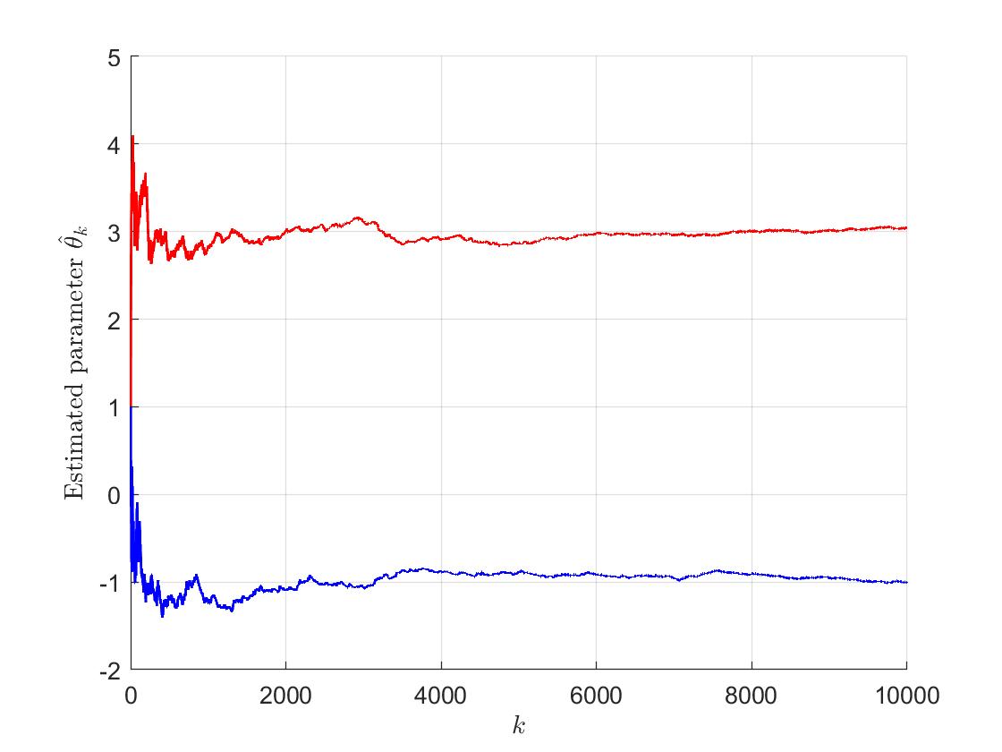
Figure 1: Convergence of Algorithm (5).

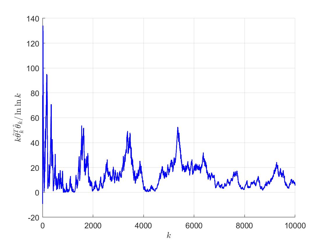
Figure 2: The trajectory of $k\lVert\tilde{\theta}_{k}\rVert^{2}/\ln\ln k$.

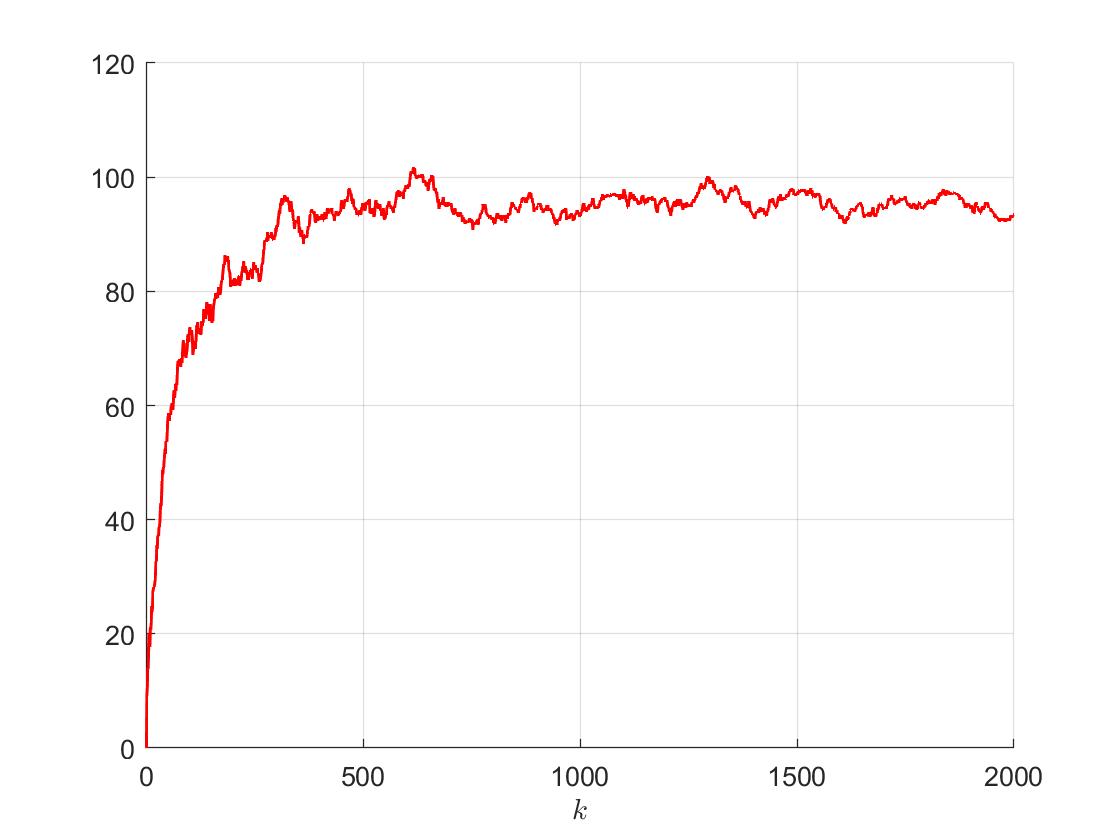
Figure 3: The trajectory of $k\lVert\tilde{\theta}_{k}\rVert^{2}$ in 200 repeated experiments.

6 Conclusion

The paper investigates the identification problem of set-valued MA systems with uniformly persistently exciting inputs. An SA-based algorithm without projection is proposed to identify the parameters. The algorithm appears to be the first online identification method for set-valued systems whose effectiveness does not rely on projections or truncations. When properly selecting the coefficients, the almost sure convergence rate of the SA-based algorithm is $O(\sqrt{\ln\ln k/k})$, and the mean square convergence rate is $O(1/k)$. Both the convergence rates are the best for the identification problem of set-valued systems in theory. Moreover, an auxiliary stochastic process named SPAO is constructed for the effectiveness analysis. The methodology can be extended to a large number of identification algorithms of set-valued systems.

Here we give some topics for future research. Firstly, the design of the step-size $\rho_{k}$ is left as an open question. How can we design a dynamic $\rho_{k}$ to allow the convergence rates to be the best automatically, and how can we design $\rho_{k}$ to make the identification algorithm achieve the Cramér-Rao lower bound asymptotically? Secondly, can the algorithm be extended to other forms of systems, e.g., nonlinear systems or systems with other kinds of nonlinear observations? And thirdly, how can we design system control laws to regulate the system performance using the SA-based algorithm?

7 Lemmas and the proofs

7.1 Proof of Lemma 1

The lemma can be indicated by Theorem 5.5.1 of [40]. We transfer the problem first.

Firstly, we claim that it is equivalent to proving that there exists $m>0$ such that $\mathbb{P}\left\{\left\|T_{k}\right\|>k^{-\varepsilon}\right\}=O\left(\exp(-mk^{1-2\varepsilon})\right)$. This is because $\sum_{j=k}^{\infty}\exp(-mj^{1-2\varepsilon})=O\left(k^{2\varepsilon}\exp(-mk^{1-2\varepsilon})\right)=O\left(\exp(-mk^{1-2\varepsilon}/2)\right)$.

Secondly, we claim that it is equivalent to prove that for any $i\in\{1,2,\ldots,n\}$, the $i$-th component of $T_{k}$, $T_{k,i}$ satisfies $\mathbb{P}\left\{\left|T_{k,i}\right|>k^{-\varepsilon}/\sqrt{n}\right\}=O\left(\exp(-mk^{1-2\varepsilon})\right)$. This is because $\left\{\left\|T_{k}\right\|>k^{-\varepsilon}\right\}\subseteq\cup_{i}\left\{\left|T_{k,i}\right|>k^{-\varepsilon}/\sqrt{n}\right\}$, which implies

$$\mathbb{P}\left\{\left\|T_{k}\right\|>k^{-\varepsilon}\right\}\leq\sum_{i=1}^{n}\mathbb{P}\left\{\left|T_{k,i}\right|>k^{-\varepsilon}/\sqrt{n}\right\}.$$

Now we have finished the transformation. The converted problem is a corollary of Theorem 5.5.1 of [40].

Lemma 3 (​[40], Theorem 5.5.1).

Assume that

1. $\{X_{k},k\geq 1\}$ is a sequence of independent random variables;

2. $\mathbb{E}X_{k}=0$ and $\left|X_{k}\right|\leq\bar{X}<\infty$;

3. $S_{k}=\sum_{i=1}^{k}X_{i}$, $\sigma_{k}=\sqrt{{\rm var}(S_{k})}$.

Then

$$\mathbb{P}\left\{\frac{S_{k}}{\sigma_{k}}>d_{k}\right\}<\max\left\{\exp\left(-\frac{d_{k}^{2}}{4}\right),\exp\left(-\frac{d_{k}\sigma_{k}}{4\bar{X}}\right)\right\}.$$

Set $X_{k,i}=\beta\phi_{k,i}\left(F_{k}-s_{k}\right)$, $S_{k,i}=\sum_{j=1}^{k}X_{j,i}$, $\sigma_{k,i}=\sqrt{\text{var}(S_{k,i})}$ and $d_{k,i}=k^{1-\varepsilon}/\sigma_{k,i}\sqrt{n}$, where $\phi_{k,i}$ is the $i$-th component of $\phi_{k}$. Then, by Lemma 3,

$$\mathbb{P}\left\{T_{k,i}>\frac{k^{-\varepsilon}}{\sqrt{n}}\right\}=\mathbb{P}\left\{\frac{S_{k,i}}{\sigma_{k,i}}>d_{k,i}\right\}$$

$$< \max\left\{\exp\left(-\frac{d_{k,i}^{2}}{4}\right),\exp\left(-\frac{d_{k,i}\sigma_{k,i}}{4\bar{X}}\right)\right\}$$

$$= \max\left\{\exp\left(-\frac{k^{2-2\varepsilon}}{4n\sigma_{k,i}^{2}}\right),\exp\left(-\frac{k^{1-\varepsilon}}{4\bar{X}\sqrt{n}}\right)\right\}.$$

Noting that

$$\sigma_{k,i}^{2}=\text{var}(S_{k,i})=\sum_{j=1}^{k}\text{var}(X_{j,i})\leq 4\bar{X}^{2}k,$$

then $\exp\left(-k^{2-2\varepsilon}/4n\sigma_{k,i}^{2}\right)\leq\exp\left(-k^{1-2\varepsilon}/16n\bar{X}^{2}\right)$. Therefore, there exists $m_{+}>0$ such that $\mathbb{P}\left\{T_{k,i}>k^{-\varepsilon}/\sqrt{n}\right\}=O\left(\exp(-m_{+}k^{1-2\varepsilon})\right)$.

$\mathbb{P}\left\{T_{k,i}<-k^{-\varepsilon}/\sqrt{n}\right\}$ can be similarly analyzed.

Combining the two consequences, the converted problem is thereby proved. That is to say, we get Lemma 1.

7.2 Lemmas in Section 4

Lemma 4.

Assume that $\phi_{k}$ satisfies Assumption 1 and the stochastic process $\psi_{k}$ satisfies $\left\|\psi_{k}-\psi_{k-1}\right\|\leq\Psi/k$ for some $\Psi>0$. Then,

$$\delta\left\|\psi_{k}\right\|^{2}\leq \frac{1}{N}\sum_{j=k+1}^{k+N}\left(\phi_{j}^{\top}\psi_{j-1}\right)^{2}+\frac{2NM^{2}\Psi}{k}\sum_{j=k}^{k+N-1}\left\|\psi_{j}\right\|$$

$$+\frac{N^{2}M^{2}\Psi^{2}}{k^{2}}.$$

Furthermore, if $b^{\prime}>0$ and $k$ is large enough, then there is $k^{\prime}\in[k+1,k+N]$ such that $\lvert\phi_{k^{\prime}}^{\top}\psi_{k^{\prime}-1}\rvert\geq\sqrt{\delta/2}\left\|\psi_{k}\right\|I_{\{\left\|\psi_{k}\right\|>b^{\prime}\}}$.

Proof.

The lemma is based on Assumption 1.

Because $\left\|\psi_{k}-\psi_{k-1}\right\|\leq\Psi/k$, $\left\|\psi_{k}-\psi_{j-1}\right\|\leq N\Psi/k$ for any $j\in[k+1,k+N]$. Therefore,

$$\frac{1}{N}\sum_{j=k+1}^{k+N}\left(\phi_{j}^{\top}\psi_{j-1}\right)^{2}$$

$$\geq \frac{1}{N}\sum_{j=k+1}^{k+N}\left(\phi_{j}^{\top}\psi_{k}\right)^{2}-\frac{2NM^{2}\Psi}{k}\sum_{j=k}^{k+N-1}\left\|\psi_{j}\right\|-\frac{N^{2}M^{2}\Psi^{2}}{k^{2}}.$$

Besides, by Assumption 1,

$$\frac{1}{N}\sum_{j=k+1}^{k+N}\left(\phi_{j}^{\top}\psi_{k}\right)^{2}=\frac{1}{N}\sum_{j=k+1}^{k+N}\psi_{k}^{\top}\phi_{j}\phi_{j}^{\top}\psi_{k}\geq\delta\left\|\psi_{k}\right\|^{2}.$$

Thus, the first part of the lemma is proved.

As for the second part, we note that under the conditions of the lemma, $\psi_{k}=O(\ln k)$. So,

$$\frac{2NM^{2}\Psi}{k}\sum_{j=k}^{k+N-1}\left\|\psi_{j}\right\|+\frac{N^{2}M^{2}\Psi^{2}}{k^{2}}=O\left(\frac{\ln k}{k}\right).$$

Hence, if $\left\|\psi_{k}\right\|>b^{\prime}$ and $k$ is sufficiently large, then one can get

$$\frac{1}{N}\sum_{j=k+1}^{k+N}\left(\phi_{j}^{\top}\psi_{j-1}\right)^{2}\geq\delta\left\|\psi_{k}\right\|^{2}+O\left(\frac{\ln k}{k}\right)>\frac{\delta}{2}\left\|\psi_{k}\right\|^{2},$$

which implies $\frac{1}{N}\sum_{j=k+1}^{k+N}\left(\phi_{j}^{\top}\psi_{j-1}\right)^{2}>\frac{\delta}{2}\left\|\psi_{k}\right\|^{2}I_{\{\left\|\psi_{k}\right\|>b^{\prime}\}}$ for sufficiently large $k$. Then, there exists $k^{\prime}\in\left[k+1,k+N\right]$ such that $\left(\phi_{k^{\prime}}^{\top}\psi_{k^{\prime}-1}\right)^{2}\geq\frac{\delta}{2}\left\|\psi_{k}\right\|^{2}I_{\{\left\|\psi_{k}\right\|>b^{\prime}\}}$, which verifies the second part of the lemma. ∎

Lemma 5.

If a sequence $a_{k}$ satisfies the recursive function

$$a_{k}\leq a_{k-1}-\frac{D\sqrt{a_{k-1}}}{k+k_{0}}I_{\{a_{k-1}\geq\frac{M^{\prime}}{2}\}}+d_{k},$$ (A.1)

where $D$, $k_{0}$ and $M^{\prime}$ are all positive, and $\sum_{k=1}^{\infty}\left|d_{k}\right|<M^{\prime}/2$, then

$$a_{k}\!<\!\max\left\{\!M^{\prime},\left[\left(\sqrt{a_{0}}-\frac{D}{2}\ln\left(\frac{k+k_{0}+1}{k_{0}+1}\right)\right)^{+}\right]^{2}\!\!\!+\frac{M^{\prime}}{2}\!\right\},$$ (A.2)

where $x^{+}=\max\{0,x\}$.

Proof.

If $a_{k}<M^{\prime}$, then the lemma is proved. Hence, we can assume that $a_{k}\geq M^{\prime}$ in the rest of the proof, which implies

$$a_{t}\geq a_{k}-\sum_{i=t+1}^{k}d_{i}\geq a_{k}-\frac{M^{\prime}}{2}\geq\frac{M^{\prime}}{2},\quad\forall t\leq k.$$

Define $a^{\prime}_{0}=a_{0}$ and $a^{\prime}_{t}=a_{t}-\sum_{i=1}^{t}\left|d_{i}\right|>M^{\prime}/2-M^{\prime}/2=0$ for $t\geq 1$. Then, we have

$$a^{\prime}_{t}= a_{t}-\sum_{i=1}^{t}\left|d_{i}\right|\leq a_{t-1}-\frac{D\sqrt{a_{t-1}}}{t+k_{0}}+d_{t}-\sum_{i=1}^{t}\left|d_{i}\right|$$

$$\leq a_{t-1}-\sum_{i=1}^{t-1}\left|d_{i}\right|-\frac{D\sqrt{\left(a_{t-1}-\sum_{i=1}^{t-1}\left|d_{i}\right|\right)^{+}}}{t+k_{0}}$$

$$= a^{\prime}_{t-1}-\frac{D\sqrt{a^{\prime}_{t-1}}}{t+k_{0}},$$

and hence,

$$a^{\prime}_{k}< a^{\prime}_{k-1}-\frac{D\sqrt{a^{\prime}_{k-1}}}{k+k_{0}}+\frac{D^{2}}{4(k+k_{0})^{2}}$$

$$= \left(\sqrt{a^{\prime}_{k-1}}-\frac{D}{2(k+k_{0})}\right)^{2},$$

which implies $\sqrt{a^{\prime}_{k}}<\sqrt{a^{\prime}_{k-1}}-\frac{D}{2(k+k_{0})}$. Therefore, by $x\leq x^{+}$

$$\sqrt{a^{\prime}_{k}}< \sqrt{a^{\prime}_{0}}-\sum_{t=1}^{k}\frac{D}{2(t+k_{0})}$$

$$\leq \left(\sqrt{a_{0}}-\frac{D}{2}\ln\left(\frac{k+k_{0}+1}{k_{0}+1}\right)\right)^{+}.$$

So,

$$a_{k}= a^{\prime}_{k}+\sum_{i=1}^{t}\left|d_{i}\right|$$

$$< \left[\left(\sqrt{a_{0}}-\frac{D}{2}\ln\left(\frac{k+k_{0}+1}{k_{0}+1}\right)\right)^{+}\right]^{2}+\frac{M^{\prime}}{2},$$

which proves the lemma. ∎

Remark 14.

Lemma 5 proves the uniform ultimate upper boundedness of the sequence $a_{k}$ which satisfies (A.1). Given the initial value $a_{0}$,

$$\sqrt{a_{0}}-\frac{D}{2}\ln\left(\frac{k+k_{0}+1}{k_{0}+1}\right)<0$$

when $k>\left(k_{0}+1\right)\exp(2\sqrt{a_{0}}/D)-k_{0}-1$, which together with (A.2) implies $a_{k}<M^{\prime}$.

Lemma 6.

Assume that

1. $v(\cdot):\mathbb{R}^{n}\to\mathbb{R}$ is a continuously twice differentiable non-negative function, whose second derivative is bounded;

2. $g_{k}(\cdot):\mathbb{R}^{n}\to\mathbb{R}^{n}$ is uniformly bounded;

3. $\nabla v(x)^{\top}g_{k}(x)$ is uniformly upper bounded, where $\nabla v(\cdot)$ is the gradient of $v(\cdot)$;

4. the positive step size $\rho_{k}\in\mathbb{R}$ satisfies $\lim\limits_{k\to\infty}\rho_{k}=0$;

5. $x_{k}=x_{k-1}+\rho_{k}g_{k}(x_{k-1})$.

Then, $v(x_{k})=O\left(\sum_{i=1}^{k}\rho_{i}\right)$.

Proof.

From

$$v(x_{k})= v(x_{k-1}+\rho_{k}g_{k}(x_{k-1}))$$

$$= v(x_{k-1})+\rho_{k}\nabla v(x_{k-1})^{\top}g_{k}(x_{k-1})+O\left(\rho_{k}^{2}\right)$$

$$\leq v(x_{k-1})+O(\rho_{k})\leq O\left(\sum_{i=1}^{k}\rho_{i}\right),$$

we get the lemma. ∎

Corollary 6.1.

Under Assumptions 1 and 2, the estimation error of Algorithm (5) satisfies $\tilde{\theta}_{k}=O\left(\sqrt{\ln k}\right)$.

Proof.

Due to the finite covariance of the noise, by Markov inequality ([36], Theorem 5.1.1), when $t$ goes to $\infty$,

$$F\left(C-\phi_{k}^{\top}\theta-t\right)= \mathbb{P}\left\{d_{k}<C-\phi_{k}^{\top}\theta-t\right\}$$

$$\leq \mathbb{P}\left\{d_{k}^{2}>\left(C-\phi_{k}^{\top}\theta-t\right)^{2}\right\}$$

$$\leq \frac{\mathbb{E}d_{k}^{2}}{\left(C-\phi_{k}^{\top}\theta-t\right)^{2}}=O\left(\frac{1}{t^{2}}\right),$$ (A.3)

and similarly, when $t$ goes to $-\infty$,

$$1-F\left(C-\phi_{k}^{\top}\theta-t\right)=O\left(\frac{1}{t^{2}}\right).$$ (A.4)

Set $v(x)=x^{\top}x$. Then, $\nabla v(x)=x$. By (A.3) and (A.4),

$$\nabla v(x)^{\top}\phi_{k}\left(F\left(C-\phi_{k}^{\top}\theta-\phi_{k}^{\top}x\right)-s_{k}\right)$$

$$= \phi_{k}^{\top}x\left(F\left(C-\phi_{k}^{\top}\theta-\phi_{k}^{\top}x\right)-s_{k}\right)$$

is uniformly upper bounded. Thus, we get the corollary by Lemma 6. ∎

Corollary 6.2.

Under the conditions of Lemma 2, $\psi_{k}=O(\sqrt{\ln k})$.

Proof.

From $\psi_{k}=\tilde{\theta}_{k}-T_{k}=O(\sqrt{\ln k})+O(1)$, we get the corollary. ∎

Remark 15.

Corollaries 6.1 and 6.2 estimate the estimation error $\tilde{\theta}_{k}$ and SPAO $\psi_{k}$ in the worst case, respectively.

Lemma 7.

For the sequence $h_{k}$, assume that

1. $h_{k}$ is positive and monotonically increasing;

2. $\ln h_{k}=o(\ln k)$.

Then, for real numbers $d$, $\eta$ and $\varepsilon$, and any positive integer $p$,

$$\sum_{l=1}^{k}\prod_{i=l+1}^{k}\left(1-\frac{\eta}{i+d}\right)^{p}\frac{h_{l}}{l^{1+\varepsilon}}=\begin{cases}O\left(\frac{h_{k}}{k^{\varepsilon}}\right),&p\eta>\varepsilon;\\ O\left(\frac{h_{k}\ln k}{k^{\varepsilon}}\right),&p\eta=\varepsilon;\\ O\left(\frac{1}{k^{p\eta}}\right),&p\eta<\varepsilon.\end{cases}$$

Proof.

By Lemma 4 in [11], we have

$$\prod_{i=l+1}^{k}\left(1-\frac{\eta}{i+d}\right)\leq\prod_{i=l+\lfloor d\rfloor+2}^{k+\lfloor d\rfloor+1}\left(1-\frac{\eta}{i}\right)=O\left(\left(\frac{l}{k}\right)^{\eta}\right),$$

which leads to

$$\sum_{l=1}^{k}\prod_{i=l+1}^{k}\left(1-\frac{\eta}{i+d}\right)^{p}\frac{h_{l}}{l^{1+\varepsilon}}= O\left(\sum_{l=1}^{k}\left(\frac{l}{k}\right)^{p\eta}\frac{h_{l}}{l^{1+\varepsilon}}\right)$$

$$= O\left(\frac{1}{k^{p\eta}}\sum_{l=1}^{k}\frac{h_{l}}{l^{1+\varepsilon-p\eta}}\right).$$

Then, it suffices to estimate $\sum_{l=1}^{k}h_{l}/l^{1+\varepsilon-p\eta}$.

Firstly, when $p\eta<\varepsilon$, by $\ln h_{k}=o(\ln k)$, we have $h_{k}<k^{(\varepsilon-p\eta)/2}$ for sufficiently large $k$, which implies $\sum_{l=1}^{\infty}\frac{h_{l}}{l^{1+\varepsilon-p\eta}}<\infty$. So, we can get

$$\sum_{l=1}^{k}\prod_{i=l+1}^{k}\left(1-\frac{\eta}{i+d}\right)^{p}\frac{h_{l}}{l^{1+\varepsilon}}=O\left(\frac{1}{k^{p\eta}}\right).$$

Secondly, by the monotonicity of $h_{k}$, we have

$$\sum_{l=1}^{k}\frac{h_{l}}{l}\leq \sum_{l=1}^{k}h_{l}\left(\ln l-\ln(l-1)\right)$$

$$\leq \sum_{l=1}^{k}\left(h_{l}\ln l-h_{l-1}\ln(l-1)\right)=h_{k}\ln k.$$

Hence, when $p\eta=\varepsilon$, one can get

$$\sum_{l=1}^{k}\prod_{i=l+1}^{k}\left(1-\frac{\eta}{i+d}\right)^{p}\frac{h_{l}}{l^{1+\varepsilon}}=O\left(\frac{h_{k}\ln k}{k^{\varepsilon}}\right).$$

Lastly, when $p\eta>\varepsilon$, we have

$$\sum_{l=1}^{k}\frac{h_{l}}{l^{1+\varepsilon-p\eta}}= O\left(\sum_{l=1}^{k}h_{l}\left(l^{p\eta-\varepsilon}-(l-1)^{p\eta-\varepsilon}\right)\right)$$

$$\leq O\left(\sum_{l=1}^{k}\left(h_{l}l^{p\eta-\varepsilon}-h_{l-1}(l-1)^{p\eta-\varepsilon}\right)\right)$$

$$= O\left(h_{k}k^{p\eta-\varepsilon}\right),$$

which implies

$$\sum_{l=1}^{k}\prod_{i=l+1}^{k}\left(1-\frac{\eta}{i+d}\right)^{p}\frac{h_{l}}{l^{1+\varepsilon}}=O\left(\frac{h_{k}}{k^{\varepsilon}}\right).$$

∎

Remark 16.

If $h_{k}$ is constant, $p=1$ and $d=0$, then Lemma 7 implies Lemma 4 in [11]. Besides, if $h_{k}/\ln k$ is assumed to be monotonically decreasing, then the estimate of Lemma 7 is accurate.

Theorem 7.

Under the conditions of Lemma 2, for any $\varepsilon\in(0,1)$, there exist positive numbers $\varepsilon^{\prime}$ and $m$ such that

$$\mathbb{P}\left\{\left\|\psi_{k}\right\|>k^{-\varepsilon^{\prime}}\right\}=O\left(\exp\left(-mk^{1-\varepsilon}\right)\right).$$

Proof.

The theorem can be proved by verifying that there exists $\varepsilon^{\prime}>0$ such that

$$\left\{\left\|\psi_{k}\right\|\leq k^{-\varepsilon^{\prime}}\right\}\supseteq\left\{\sup_{j\geq\lfloor k^{1-2\varepsilon}\rfloor}j^{\varepsilon}\left\|T_{j}\right\|\leq 1\right\}.$$ (A.5)

By the monotonicity of $\{\sup_{j\geq k}j^{\varepsilon}\left\|T_{j}\right\|\leq 1\}$ and Theorem 1,

$$\left\{\sup_{j\geq\lfloor k^{1-\varepsilon}\rfloor}\lVert\psi_{j}\rVert^{2}<M^{\prime}\right\}\supseteq\left\{\sup_{j\geq\lfloor k^{1-2\varepsilon}\rfloor}j^{\varepsilon}\left\|T_{j}\right\|\leq 1\right\}.$$

Therefore, if $\sup_{j\geq\lfloor k^{1-2\varepsilon}\rfloor}j^{\varepsilon}\left\|T_{j}\right\|\leq 1$, then by (4.3) and (4.3), for all $j\geq\lfloor k^{1-\varepsilon}\rfloor+N$,

$$\left\|\psi_{j}\right\|\leq\left(1-\frac{\beta\delta N}{j}\underline{f}\left(M\sqrt{M^{\prime}}\right)\right)\left\|\psi_{j-N}\right\|+O\left(\frac{1}{j^{1+\varepsilon}}\right),$$

where $\underline{f}(\cdot)$ is defined in (10). Then, by Corollaries 6.2 and 7, $\left\|\psi_{j}\right\|$ converges at a polynomial rate. Hence, we get (A.5). Then, the theorem can be proved by Lemma 1 and the arbitrariness of $\varepsilon$. ∎

Corollary 7.1.

Under the conditions of Theorem 2, for any $\varepsilon>0$, there exist positive numbers $\varepsilon^{\prime}$ and $m$ such that

$$\mathbb{P}\left\{\lVert\tilde{\theta}_{k}\rVert>k^{-\varepsilon^{\prime}}\right\}=O\left(\exp\left(-mk^{1-\varepsilon}\right)\right).$$

Proof.

By (A.5) and $\tilde{\theta}_{k}=\psi_{k}+T_{k}$, we have

$$\left\{\lVert\tilde{\theta}_{k}\rVert^{2}\leq k^{-\varepsilon^{\prime}}+k^{-\varepsilon}\right\}\supseteq \left\{\left\|\psi_{k}\right\|\leq k^{-\varepsilon^{\prime}}\right\}\cap\left\{\left\|T_{k}\right\|\leq k^{-\varepsilon}\right\}$$

$$\supseteq \left\{\sup_{j\geq\lfloor k^{1-2\varepsilon}\rfloor}j^{\varepsilon}\left\|T_{j}\right\|\leq 1\right\}.$$

Then, the corollary can be proved by Lemma 1. ∎

Remark 17.

Theorems 7 and 7.1 are extensions of Theorems 1 and 2, respectively.

8 SPAO for other algorithms

The construction of SPAO can be applied to many online identification algorithms of set-valued systems. For set-valued systems with threshold $C_{k}$, a large number of recursive identification algorithms can be represented as

$$\hat{\theta}_{k}=\hat{\theta}_{k-1}+\rho_{k}v_{k}\left(h(\phi_{k},\hat{\theta}_{k-1})-s_{k}\right),$$

where $\{\phi_{k},k\geq 1\}$ are independent regressed function of inputs, $C_{k}$ and $v_{k}$ are generated by $\{\phi_{j},s_{j-1},j\leq k\}$ [18, 31, 19, 9, 32, 20, 33, 30, 29]. The step size $\rho_{k}$ can also be matrices [32, 33].

Define $\psi_{k}=\tilde{\theta}_{k}-T_{k}$, where $\tilde{\theta}_{k}=\hat{\theta}_{k}-\theta$ is the estimation error and

$$T_{k}= \rho_{k}\left(\sum_{i=1}^{k}v_{i}\left(\mathbb{E}\left[s_{i}|\phi_{j},s_{j-1},j\leq i\right]-s_{i}\right)\right)$$

$$= \rho_{k}\left(\sum_{i=1}^{k}v_{i}\left(F(C_{i}-\phi_{i}^{\top}\theta)-s_{i}\right)\right).$$

Then, one can get

$$\psi_{k}= \psi_{k-1}+\rho_{k}v_{k}\left(h(\phi_{k},\psi_{k-1}+T_{k-1})-F(C_{k}-\phi_{k}^{\top}\theta)\right)$$

$$+\rho_{k}\left(\rho_{k}^{-1}-\rho_{k-1}^{-1}\right)T_{k-1}.$$

If there is a good convergence property for $T_{k}$, then the trajectory of $\psi_{k}$ is similar to that of $\tilde{\theta}_{k}$ and that of the deterministic sequence

$$\overline{\psi}_{k}=\overline{\psi}_{k-1}+\rho_{k}v_{k}\left(h(\phi_{k},\overline{\psi}_{k-1})-F(C_{k}-\phi_{k}^{\top}\theta)\right).$$

Therefore, we can analyze the convergence property of the algorithm through SPAO $\psi_{k}$.

[]Jieming Ke(S’22) received the B.S. degree in Mathematics from University of Chinese Academy of Science, Beijing, China, in 2020. He is currently working toward the Ph.D. degree majoring in system theory at Academy of Mathematics and Systems Science, Chinese Academy of Science, Beijing, China.

His research interests include identification and control of set-valued systems and the information security problems of control systems.

[]Ying Wang(S’20-M’22) received the B.S. degree in Mathematics from Wuhan University, Wuhan, China, in 2017, and the Ph.D. degree in systems theory from the Academy of Mathematics and Systems Science (AMSS), Chinese Academy of Sciences (CAS), Beijing, China, in 2022. She is currently a Post-Doctoral Research Associate in AMSS, CAS.

Her research interests include identification and adaptive control of quantized systems, and distributed estimation and adaptive control of multi-agent systems.

[]Yanlong Zhao(S’07-SM’18) received the B.S. degree in mathematics from Shandong University, Jinan, China, in 2002, and the Ph.D. degree in systems theory from the Academy of Mathematics and Systems Science (AMSS), Chinese Academy of Sciences (CAS), Beijing, China, in 2007. Since 2007, he has been with the AMSS, CAS, where he is currently a full Professor. His research interests include identification and control of quantized systems, information theory and modeling of financial systems.

He has been a Deputy Editor-in-Chief Journal of Systems and Science and Complexity, an Associate Editor of Automatica, SIAM Journal on Control and Optimization, and IEEE Transactions on Systems, Man and Cybernetics: Systems. He served as a Vice-President of Asian Control Association, and is now a Vice General Secretary of Chinese Association of Automation (CAA), a Vice-Chair of Technical Committee on Control Theory (TCCT), CAA, and a Vice-President of IEEE CSS Beijing Chapter.

[]Ji-Feng Zhang(M’92-SM’97-F’14) received the B.S. degree in mathematics from Shandong University, China, in 1985, and the Ph.D. degree from the Institute of Systems Science (ISS), Chinese Academy of Sciences (CAS), China, in 1991. Since 1985, he has been with the ISS, CAS. His current research interests include system modeling, adaptive control, stochastic systems, and multi-agent systems.

He is an IEEE Fellow, IFAC Fellow, CAA Fellow, SIAM Fellow, member of the European Academy of Sciences and Arts, and Academician of the International Academy for Systems and Cybernetic Sciences. He received the Second Prize of the State Natural Science Award of China in 2010 and 2015, respectively. He is a Vice-President of the Chinese Mathematical Society and the Chinese Association of Automation. He was a Vice-Chair of the IFAC Technical Board, member of the Board of Governors, IEEE Control Systems Society; Convenor of Systems Science Discipline, Academic Degree Committee of the State Council of China; Vice-President of the Systems Engineering Society of China. He served as Editor-in-Chief, Deputy Editor-in-Chief or Associate Editor for more than 10 journals, including Science China Information Sciences, IEEE Transactions on Automatic Control and SIAM Journal on Control and Optimization etc.

References

[1]
L. Y. Wang, Y. W. Kim, and J. Sun, “Prediction of oxygen storage capacity and stored NOx by HEGO sensors for improved LNT control strategies,” in ASME International Mechanical Engineering Congress and Exposition, 2002, pp. 777–785.
[2]
L. Y. Wang, J. F. Zhang, and G. G. Yin, “System identification using binary sensors,” IEEE Trans. Automa. Control, vol. 48, no. 11, pp. 1892–1907, 2003.
[3]
L. Y. Wang, G. G. Yin, J. F. Zhang, and Y. L. Zhao, System Identification with Quantized Observations, Boston, MA, USA: Birkhäuser, 2010.
[4]
G. Kang, W. Bi, H. Zhang, S. B. Pounds, C. Cheng, S. Shete, F. Zou, Y. L. Zhao, J. F. Zhang, W. Yue, “A robust and powerful set-valued approach to rare variant association analyses of secondary traits in case-control sequencing studies,” Genetics, vol. 205, no. 3, pp. 1049–-1062, 2017.
[5]
W. Bi, W. Zhou, R. Dey, B. Mukherjee, J. N. Sampson, S. Lee, “Efficient mixed model approach for large-scale genome-wide association studies of ordinal categorical phenotypes,” Am. J. Hum. Genet., vol. 108, no. 5, pp. 825–839, 2021.
[6]
T. Wang, W. Bi, Y. L. Zhao, and W. Xue, “Radar target recognition algorithm based on RCS observation sequence—set-valued identification method,” J. Syst. Sci. Complex., vol. 29, pp. 573–588, 2016.
[7]
X. Wang, M. Hu, Y. L. Zhao, B. Djehiche, “Credit scoring based on the set-valued identification method,” J. Syst. Sci. Complex., vol. 33 , pp. 1297–1309, 2020.
[8]
X. Li, Z. Xu, J. Cui, and L. Zhang, “Suboptimal adaptive tracking control for FIR systems with binary-valued observations,” Sci. China Inf. Sci., vol. 64, 2021, Art. no. 172202.
[9]
T. Wang, M. Hu, and Y. L. Zhao, “Adaptive tracking control of FIR systems under binary-valued observations and recursive projection identification,” IEEE Trans. Syst., Man, Cybern., Syst., vol. 51, no. 9, pp. 5289–5299, 2021.
[10]
Y. L. Zhao, J. Guo, and J. F. Zhang, “Adaptive tracking control of linear systems with binary-valued observations and periodic target,” IEEE Trans. Automa. Control, vol. 58, no. 5, pp. 1293–1298, 2013.
[11]
Y. L. Zhao, T. Wang, and W. Bi, “Consensus protocol for multi-agent systems with undirected topologies and binary-valued communications,” IEEE Trans. Automa. Control, vol. 64, no. 1, pp. 206–221, 2019.
[12]
G. Bottegal, H. Hjalmarsson, and G. Pillonetto, “A new kernel-based approach to system identification with quantized output data,” Automatica, vol. 85, pp. 145–152, 2017.
[13]
E. Colinet and J. Juillard, “A weighted least-squares approach to parameter estimation problems based on binary measurements,” IEEE Trans. Automa. Control, vol. 55, no. 1, pp. 148–152, 2010.
[14]
B. I. Godoy, G. C. Goodwin, J. C. Agüero, D. Marelli, and T. Wigren, “On identification of FIR systems having quantized output data,” Automatica, vol. 47, no. 9, pp. 1905–1915, 2011.
[15]
F. Gustafsson and R. Karlsson, “Statistical results for system identification based on quantized observations,” Automatica, vol. 45, no. 12, pp. 2794–2801, 2009.
[16]
R. S. Risuleo, G. Bottegal, and H. Hjalmarsson, “Identification of linear models from quantized data: A midpoint-projection approach,” IEEE Trans. Automa. Control, vol. 65, no. 7, pp. 2801–2813, 2020.
[17]
X. Shen, P. K. Varshney, and Y. Zhu, “Robust distributed maximum likelihood estimation with dependent quantized data,” Automatica, vol. 50, no. 1, pp. 169–174, 2014.
[18]
B. C. Csáji and E. Weyer, “Recursive estimation of ARX systems using binary sensors with adjustable thresholds,” in 16th IFAC Symposium on
System Identification, 2012, pp. 1185–1190.
[19]
Q. Song, “Recursive identification of systems with binary-valued outputs and with ARMA noises,” Automatica, vol. 93, pp. 106–113, 2018.
[20]
K. You, “Recursive algorithms for parameter estimation with adaptive quantizer,” Automatica, vol. 52, pp. 192–201, 2015.
[21]
J. D. Diao, J. Guo, and C. Sun, “A compensation method for the packet loss deviation in system identification with event-triggered binary-valued observations,” Sci. China Inf. Sci., vol. 63, no. 12, 2020, Art. no. 229204.
[22]
Q. He, G. G. Yin, and L. Y. Wang, “Moderate deviations analysis for system identification under regular and binary observations,” in 2013 Proceedings of the Conference on Control and its Applications (CT), 2013, pp. 51–58.
[23]
H. Mei, L. Y. Wang, and G. Yin, “Almost sure convergence rates for system identification using binary, quantized, and regular sensors,” Automatica, vol. 50, no. 8, pp. 2120–2127, 2014.
[24]
A. Moschitta, J. Schoukens, and P. Carbone, “Parametric system identification using quantized data,” IEEE Trans. Instrum. Meas., vol. 64, no. 8, pp. 2312–2322, 2015.
[25]
L. Y. Wang and G. G. Yin, “Asymptotically efficient parameter estimation using quantized output observations,” Automatica, vol. 43, no. 7, pp. 1178–1191, 2007.
[26]
L. Y. Wang, G. G. Yin, and J. F. Zhang, “Joint identification of plant rational models and noise distribution functions using binary-valued observations,” Automatica, vol. 42, no. 4, pp. 535–547, 2006.
[27]
L. Y. Wang, G. G. Yin, Y. L. Zhao, and J. F. Zhang, “Identification input design for consistent parameter estimation of linear systems with binary-valued output observations,” IEEE Trans. Automa. Control, vol. 53, no. 4, pp. 867–880, 2008.
[28]
Y. L. Zhao, J. F. Zhang, L. Y. Wang, and G. G. Yin, “Identification of Hammerstein systems with quantized observations,” SIAM J. Control Optim., vol. 48, no. 7, pp. 4352–4376, 2010.
[29]
K. Fu, H. F. Chen, W. X. Zhao, “Distributed system identification for linear stochastic systems with binary sensors,” Automatica, vol. 141, 2022, Art. no. 110298.
[30]
Y. Wang, Y. L. Zhao, J. F. Zhang, J. Guo, “A unified identification algorithm of FIR systems based on binary observations with time-varying thresholds,” Automatica, vol. 135, 2022, Art. no. 109990.
[31]
J. Guo and Y. L. Zhao, “Recursive projection algorithm on FIR system identification with binary-valued observations,” Automatica, vol. 49, no. 11, pp. 3396–3401, 2013.
[32]
Y. Wang, Y. L. Zhao, and J. F. Zhang, “Distributed recursive projection identification with binary-valued observations,” J. Syst. Sci. Complex., vol. 34, no. 5, pp. 2048–2068, 2021.
[33]
H. Zhang, T. Wang, and Y. L. Zhao, “Asymptotically efficient recursive identification of FIR systems with binary-valued observations,”
IEEE Trans. Syst., Man, Cybern., Syst., vol. 51, no. 5, pp. 2687–2700, 2021.
[34]
H. F. Chen and L. Guo, “Adaptive control via consistent estimation for deterministic systems,” Int. J. of Contr., vol. 45, no. 6, pp. 2183–2202, 1987.
[35]
H. F. Chen, Stochastic Approximation and Its Applications, vol. 64, New York, USA: Springer Science & Business Media, 2006.
[36]
Y. S. Chow and H. Teicher, Probability Theory: Independence, Interchangeability, Martingales, New York, USA: Springer Science & Business Media, 1997.
[37]
V. Fabian, “On asymptotic normality in stochastic approximation,” Ann. Math. Stat., vol. 39, no. 4, pp. 1327–1332, 1968.
[38]
V. A. Zorich, Mathematical Analysis I, Berlin, Germany: Universitext, Springer-Verlag, 2016.
[39]
L. Guo, Introduction to control theory: from basic concepts to research frontier, Beijing, China: Science Press, 2005.
[40]
H. G. Tucker, A Graduate Course in Probability, New York, USA: Academic Press, 1967.
{IEEEbiography}