Lightweight Facial Attractiveness Prediction
Using Dual Label Distribution

Abstract

Facial attractiveness prediction (FAP) aims to assess the facial attractiveness automatically based on human aesthetic perception. Previous methods using deep convolutional neural networks have boosted the performance, but their giant models lead to a deficiency in flexibility. Besides, most of them fail to take full advantage of the dataset. In this paper, we present a novel end-to-end FAP approach integrating dual label distribution and lightweight design. To make the best use of the dataset, the manual ratings, attractiveness score, and standard deviation are aggregated explicitly to construct a dual label distribution, including the attractiveness distribution and the rating distribution. Such distributions, as well as the attractiveness score, are optimized under a joint learning framework based on the label distribution learning (LDL) paradigm. As for the lightweight design, the data processing is simplified to minimum, and MobileNetV2 is selected as our backbone. Extensive experiments are conducted on two benchmark datasets, where our approach achieves promising results and succeeds in striking a balance between performance and efficiency. Ablation studies demonstrate that our delicately designed learning modules are indispensable and correlated. Additionally, the visualization indicates that our approach is capable of perceiving facial attractiveness and capturing attractive facial regions to facilitate semantic predictions.

I Introduction

Facial attractiveness plays a significant role in our daily life. Since the discovery of golden ratio and the Facial Fifths and Thirds, researchers from different disciplines have devoted themselves to decrypt the mysterious facial aesthetics. Psychology studies have shown that people with attractive faces are more likely to enjoy higher social status, preferential employment, and professional achievement [1, 2, 3]. Facial attractiveness prediction (FAP) aims to assess facial attractiveness automatically based on human aesthetic perception, which is related to various real-life applications, such as face beautification [4, 5], facial expression recognition [6], personalized social recommendation [7], and cosmetic surgery [8].

In the past two decades, FAP has gradually become a prosperous research topic in computer vision. The methods can be categorized into handcrafted feature based and deep learning based. In most early studies, low-level features like geometric [9, 10] and texture descriptors [11, 12] are manually designed. Such representation, however, may lack discriminative capability, resulting in poor performance. With the booming of deep learning, numerous convolutional neural networks (CNN) [13, 14, 15] have been applied to FAP. Due to the powerful nonlinearity, CNN-based methods are able to learn hierarchical aesthetic representation, and have achieved superior performance over traditional methods.

Previous FAP methods using deep CNNs have boosted the performance, but their giant models lead to a lack of flexibility. Adapting neural network architectures to strike a balance between performance and efficiency has been an active research field in recent years. Through manual or automatic architecture design, different architectures have been developed for resource-constrained devices, e.g., SqueezeNet [16], MobileNet [17, 18, 19, 20], and EfficientNet [21]. These backbones have been widely used in classification [22], recognition [23] and object detection [24]. However, FAP has paid little attention to such lightweight architecture. The only work utilizing lightweight backbone is to employ MobileNetV2 with co-attention learning mechanism [25].

The FAP datasets usually include facial images with their corresponding manual ratings, ground-truth scores, and standard deviations. Therefore, among CNN-based methods, several labeling schemes have been adopted to meet different learning objectives and employ the dataset to varying degrees. The single-label (average score) is the most commonly used, but only takes one type of label into consideration, thus imposing strong restrictions to learning. Although the multi-label scheme cannot well adapt to FAP, its variant, i.e., label distribution learning (LDL), has been introduced to provide a novel view of attractiveness learning [26]. Human ratings are aggregated into the label distribution, while the ground-truth score and standard deviation fail to be utilized explicitly. It is notable that the LDL paradigm was formally proposed by Geng [27], which aims to learn the latent distributions in the dataset. Since then, it has been applied to various tasks, such as age estimation [28], emotion distribution recognition [29], and facial landmark detection [30].

In this paper, we present a novel end-to-end FAP approach consisting of the dual label distribution and joint learning framework based on lightweight design. The lightweight design lies in many aspects, from data processing to backbone selection. We have simplified the data preprocessing and augmentation to minimum, and have conducted extensive experiments to reach the final decision to employ MobileNetV2 as our backbone. To make the best use of the dataset, the dual label distribution, including the attractiveness distribution and rating distribution, is proposed and constructed to utilize the manual ratings, ground-truth score, and standard deviation, explicitly. Then, it is fed into the MobileNetV2 for joint learning, which is designed to optimize three learning modules simultaneously based on the LDL paradigm. The attractiveness distribution learning module aims to optimize the network output directly, namely the predicted attractiveness distribution. The rating distribution learning module is designed to refine the predicted rating distribution, meanwhile performing further supervision to learning process. The score regression learning module concentrates on further refining the predicted attractiveness score with a novel loss. Finally, given a facial image, the trained model outputs its predicted attractiveness distribution and obtains its attractiveness score so as to accomplish end-to-end FAP. The framework of our approach is presented in Fig. 1.

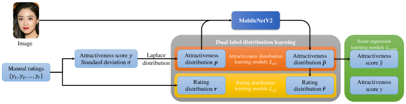
Figure 1: The overview of our framework. For a given facial image, its manual ratings, attractiveness score, and standard deviation are aggregated explicitly. With the human ratings $\{y_{1},y_{2},\dots,y_{r}\}$, its attractiveness distribution $\boldsymbol{p}$ is generated using the Laplace distribution, while its rating distribution $\boldsymbol{r}$ is derived directly. Then, the facial image and $\boldsymbol{p}$ are fed into the MobileNetV2 to output the predicted attractiveness distribution $\hat{\boldsymbol{p}}$, which is utilized subsequently to compute the predicted attractiveness score $\hat{y}$ and obtain the predicted rating distribution $\hat{\boldsymbol{r}}$. Finally, $\hat{\boldsymbol{p}}$, $\hat{\boldsymbol{r}}$ and $\hat{y}$ are jointly optimized under the dual label distribution and score regression learning modules.

The contributions of this paper are summarized as follows.

• We present a novel end-to-end FAP approach incorporating the dual label distribution and three learning modules. To the best of our knowledge, this is the first to leverage the lightweight design and LDL paradigm to predict facial attractiveness.

• The dual label distribution is proposed to take full advantage of the dataset, including the manual ratings, ground-truth score, and standard deviation. We further present the joint learning framework to optimize the dual label distribution and concurrently refine the predictions using a novel loss.

• Extensive experiments are conducted on two benchmarks, where our approach achieves appealing results with greatly decreased parameters and computation. Moreover, our framework is capable of perceiving facial attractiveness so as to facilitate semantic predictions.

II Related Work

II-A Deep Learning Based Facial Attractiveness Prediction

The handcrafted feature based methods advanced the field and brought some early success. However, such methods suffer from multiple limitations. First, they are dependent on low-level features which lack representational capability, leading to inferior performance. Second, the model performance relies heavily on the feature selection. Third, the process of feature selection can be really complicated and highly empirical. Lastly, the handcrafted features are strongly constrained because most of them are based on existing aesthetic criteria or findings from psychological research.

With the booming of deep learning, a substantial amount of CNN-related works have been proposed, many of which have obtained remarkable results on some challenging visual classification or recognition tasks [31, 32]. Meanwhile, the effectiveness of CNN with its variants have been extensively explored in facial attractiveness prediction. Gray et al. [13] were the first to construct a CNN-like hierarchical feed-forward model to extract attractiveness features for FAP. Xie et al. [33] designed a six-layer CNN to learn the features in multiple levels and directly output the attractiveness score. Later, VGG network [34] was proposed to extract discriminative deep facial features, which were then utilized for attractiveness prediction [35]. To a certain extent, deeper architectures enable the extraction of more discriminative and representative features. Simultaneously, researchers have been seeking other paths for enhanced performance and more general solutions. Xu et al. [36] were inspired by psychology to propose a cascaded CNN (PI-CNN) for FAP and fine-tuned with different aesthetic features. Inspired by the effectiveness of facial attributes on facial attractiveness, Lin et al. [15] proposed an attribute-aware CNN (AaNet) that can integrate attractiveness-related attributes into feature representation so as to modulate the filters of the network adaptively. Most recently, Lin et al. [14] redefined facial attractiveness prediction as a ranking guided regression task, proposed an algorithm guided by relative aesthetic, and constructed a ranking guided CNN (R³CNN), which is able to accomplish ranking and regression simultaneously. Bougourzi et al. [37] first proposed a two-branch architecture named REX-INCEP by combining two trained networks, and established an ensemble regressor (CNN-ER) for FAP employing multiple dynamic loss functions, which consists of 6 models involving the proposed REX-INCEP. In addition, facial attractiveness prediction can be collaborated with other visual tasks. Xu et al. [38] designed a hierarchical multi-task network that can simultaneously output the gender, race and facial attractiveness of a given portrait image. Recently, Xu [39] proposed a multi-task FAP model to automatically conduct facial attractiveness and gender prediction.

II-B Lightweight Architecture

The model efficiency is often a vital indicator in deep learning tasks, which is measured by the number of trainable parameters, floating point operations per second (FLOPs), and multiply-adds (MAdds) [18]. In recent years, extensive studies have made efforts to adapt neural network architecture to strike a balance between model efficiency and performance, i.e., reducing the amount of model parameters or MAdds while maintaining relatively high performance in multiple tasks, such as SqueezeNet, EfficientNet, and MobileNet. SqueezeNet was presented based on a more disciplined method exploring the design-space of CNNs proposed by Iandola et al., which has 50$\times$ fewer parameters than AlexNet and accomplishes AlexNet-level accuracy on ImageNet [16]. Tan and Le [21] designed a new baseline network using neural architecture search, which was then scaled up to a family of EfficientNets utilizing the proposed scaling method that uniformly scales all dimensions of depth, width, and resolution. The EfficientNets achieved state-of-the-art performance on ImageNet, while being much smaller and faster on inference stage. The MobileNet variants largely depend on separable convolutions to decrease the model size, which decompose standard convolutions into a 1$\times$1 pointwise convolution and a depthwise convolution applied to each channel separately. MobileNetV1 [17] is based on a streamlined architecture which uses depth-wise separable convolutions. MobileNetV2 [18] utilizes the proposed linear bottleneck with an inverted residual structure. Later, MobileNetV3 [19] was developed through hardware-aware network architecture search, which adopts squeeze and excitation, and nonlinearities like swish. Recently, Zhou et al. [20] presented a bottleneck named sandglass block based on the disadvantage analysis of the inverted residual block in MobileNetV2, which was employed to construct MobileNeXt.

The aforementioned lightweight architectures have been broadly employed in multiple tasks, like the popular classification and object detection. Xie et al. [22] presented a concise self-training method for ImageNet classification, which iteratively trains a smaller and a larger EfficientNet models being student and teacher in turns. Tan et al. [24] developed a novel family of object detectors named EfficientDet based on EfficientNet backbones and several optimizations for object detection, including a weighted bidirectional feature pyramid network and a compound scaling method. In addition to employing lightweight backbones directly, many researchers have been dedicated to develop models for various tasks based on the lightweight design idea. Song et al. [40] transferred the separable convolutions proposed in MobileNets to construct an efficient graph convolutional network for skeleton-based action recognition. Most recently, Sun et al. [41] borrowed the first layer and the first convolutional linear bottleneck of MobileNetV2 as feature extractor in their proposed lightweight single-image segmentation network.

Although lightweight design has been widely adopted in many tasks, the field of FAP has largely ignored it and few related studies have been carried out. Shi et al. [25] proposed to enhance prediction by utilizing pixel-wise labeling masks for accurate facial composition, and co-attention learning mechanism with MobileNetV2.

II-C Label Distribution Learning

Previous learning paradigms cannot well suit some real applications in which the overall distribution of the labels matters. Besides, there exists real-world data with natural measures of the labels’ importance. Therefore, motivated by the above facts, label distribution learning was formally proposed by Geng in 2016 [27], which is a more general learning framework than single-label and multi-label learning. It concentrates on the ambiguity on the label side, aiming to learn the latent distribution of the labels. Generally speaking, the label distribution involves a certain number of labels, and each label describes the importance to the instance.

Label distribution learning has been adopted in a wide range of tasks. To tackle the issue of treating the facial expression of an image as merely a single emotion, Zhou et al. [29] proposed the emotion distribution learning method to output the intensity of all basic emotions on a given image so as to achieve facial expression recognition. To alleviate the expensive computation of giant models and the inconsistency between the training and evaluation phase, Gao et al. [28, 42] designed a lightweight architecture and developed a unified framework to jointly learn age distribution and regress age using the expectation of age distribution. Su and Geng [30] developed a soft facial landmark detection algorithm motivated by the inaccurately annotated landmarks. The algorithm associates each landmark with a bivariate label distribution (BLD), learns the mappings from an image patch to the BLD for each landmark, and finally obtains the facial shape based on the predicted BLDs.

In addition to the aforementioned works, label distribution learning has also been employed in the field of facial attractiveness prediction. Ren and Geng [43] proposed a method named Beauty Distribution Transformation to convert the $k$-wise ratings to label distribution, and a learning method called Structural Label Distribution Learning based on structural support vector machine to reveal the human sense of facial attractiveness. Our previous work [26] utilized the inherent score distribution of each image given by human raters as the learning objective, and integrated low-level geometric features with high-level CNN features to accomplish automatic attractiveness computation. Later, Chen and Deng [44] developed Deep Adaptive Label Distribution Learning framework, utilizing discrete label distribution of possible ratings to supervise the learning process of FAP. Recently, Gao et al. [42] presented deep label distribution learning-v2 (DLDL-v2) approach, which was originated from age estimation [28], and designed the lightweight ThinAttNet and TinyAttNet to estimate facial attractiveness based on the expectation of label distribution.

III Dual Label Distribution

Our proposed approach is introduced in the following sections, which consists of the dual label distribution and its learning scheme. In this section, we present the construction of the dual label distribution. First, some preliminaries are introduced to lay the foundation. Then, the dual label distribution is proposed in detail, including the rating distribution and the attractiveness distribution.

III-A Preliminaries

III-A1 The Facial Attractiveness Prediction Problem

Assume that a training set with $N$ samples is denoted as $\{(x^{(i)},y^{(i)})\}^{N}_{i=1}$, where $x^{(i)}$ and $y^{(i)}$ denote the $i$-th image and its ground-truth score (average score). We might omit the superscript $(i)$ for simplicity. The goal of facial attractiveness prediction is to learn a mapping from facial images to attractiveness scores such that the error between the predicted score $\hat{y}$ and ground-truth score $y$ be as small as possible on an input image $x$.

III-A2 Laplace Distribution

The construction of attractiveness distribution is based on the Laplace distribution. Defined by the location parameter $\mu$ and the scale parameter $b$ (their settings for each image will be introduced in Section III-C), the probability density function of the Laplace distribution is

$$f(x|\mu,b)=\frac{1}{2b}\exp(-\frac{|x-\mu|}{b})$$ (1)

while the cumulative distribution function is

$$F(x|\mu,b)=\frac{1}{2}[1+\text{sgn}(x-\mu)(1-\exp(-\frac{|x-\mu|}{b}))]$$ (2)

where the mean and standard deviation of the distribution are $\mu$ and $\sqrt{2}b$, respectively.

During training phase, the attractiveness distribution is fed into the model, and the rating distribution is employed for supervision. Their generation is introduced in the following.

III-B Rating Distribution

In our previous work[26], a facial attractiveness prediction method based on LDL was proposed, which utilized the rating records directly to derive the rating distribution. The ground-truth score and standard deviation, however, were implicitly included, thus ignoring their importance. We follow the same way to construct the rating distribution, represented by the vector $\boldsymbol{r}$.

Let $r_{m}$ be the number of raters who rated the image with the attractiveness score $m$. Since the attractiveness score is an integer ranging from 1 to 5, $m=\{1,2,3,4,5\}$. Then, $L_{1}$ normalization is applied to $\boldsymbol{r}$ such that $\sum_{m=1}^{5}r_{m}=1$. We can see that $\boldsymbol{r}$ represents the actual rating distribution of the image.

III-C Attractiveness Distribution

In order to utilize the ground-truth score $y$ and the standard deviation $\sigma$ of the image explicitly, the attractiveness distribution are constructed, which takes the advantage of LDL and is represented by the vector $\boldsymbol{p}$.

The formation of $\boldsymbol{p}$ is introduced as follows. Each element of $\boldsymbol{p}$ represents the probability of the attractiveness score on a certain interval. These probabilities are then combined to establish the attractiveness distribution. First, we define the interval endpoints $s_{k}$

$$s_{k}=y_{\min}+k\cdot\Delta l$$ (3)

where $y_{\min}$ and $\Delta l$ are the minimum attractiveness score and interval length, respectively.

Then, the $j$-th interval $I_{j}$ is formed as

$$I_{j}=[s_{j},s_{j+1}]$$ (4)

Its corresponding probability $p_{j}$, namely the $j$-th element of $\boldsymbol{p}$, is calculated using the cumulative distribution function of the Laplace distribution $F(x|\mu,b)$.

$$p_{j}=F(s_{j+1}|\mu,b)-F(s_{j}|\mu,b)$$ (5)

where the location parameter and scale parameter are set to $\mu=y$ and $b=\frac{\sigma}{\sqrt{2}}$ for each image, which is consistent with the mathematical definition, thereby the construction is logical and expected to be viable.

In this work, the interval length $\Delta l$ is 0.1. To make the best choice of $\Delta l$, we have conducted a series of comparative experiments with $\Delta l=\{0.01,0.05,0.1,0.2,0.5\}$, and have found that either larger or smaller $\Delta l$ would pose negative impact on performance. Concretely, with larger $\Delta l$, the model outputs sparser representation of the attractiveness distribution, which would directly decreases its precision and further affects the derived rating distribution. On the other hand, with smaller $\Delta l$, the model has to output distribution with higher dimensions, which is definitely a challenge for the lightweight architecture due to its limited representational power.

Since the attractiveness score ranges from 1 to 5 in our adopted datasets, $s_{k}$ should share the identical range. Let $y_{\max}$ and $y_{\min}$ be the maximum and minimum attractiveness score respectively, then $y_{\min}=1$ and $y_{\max}=5$. Notice that $s_{k}$, $I_{j}$, and $p_{j}$ are 0-indexed. We have $k_{\max}=(y_{\max}-y_{\min})/\Delta l=40$. Hence, in Eqs. (3)-(5), $k\in[0,40],j\in[0,39]$.

Finally, we perform element-wise sigmoid operation and $L_{1}$ normalization to $\boldsymbol{p}$. The sigmoid operation offers nonlinear variation to $\boldsymbol{p}$, enhancing its representational power. The $L_{1}$ normalization is performed such that $\sum_{j=0}^{39}p_{j}=1$, hence satisfying the general property of a probability distribution.

IV Learning

In this section, we continue to present our approach following Section III. The employed network architecture and the proposed joint learning framework are introduced in detail.

IV-A Network Architecture

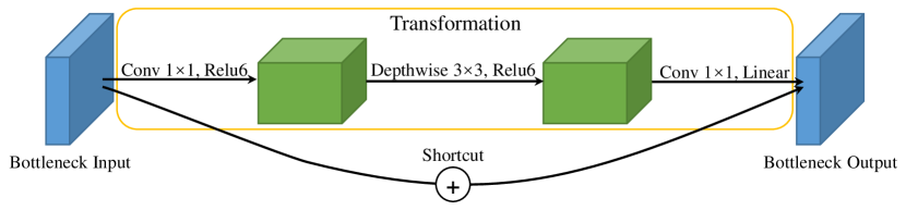
Figure 2: The building block of MobileNetV2, which consists of the linear bottlenecks and an inverted residual structure.

Considering the balance between performance and efficiency, MobileNetV2 [18] is selected as our backbone after extensive experiments. As shown in Fig. 2, the building block of MobileNetV2 includes a 1$\times$1 expansion convolution, depthwise convolutions followed by a 1$\times$1 projection layer. The narrow input and output (bottleneck) are connected with a residual connection. This structure greatly reduces model size and computation while maintaining a relatively high performance on multiple tasks. Besides, sigmoid operation and $L_{1}$ normalization are also conducted on the output so as to reduce the inconsistency between the input and output.

IV-B Joint Learning Framework

The joint learning framework contains attractiveness distribution, rating distribution and score regression learning modules. As shown in Fig. 1, the input image with its attractiveness distribution are fed into the MobileNetV2 to jointly optimize dual label distribution and attractiveness score in an end-to-end manner.

IV-B1 Attractiveness Distribution Learning

The Kullback-Leibler divergence is commonly used in the scenario of measuring how two probability distributions differ from each other [26, 28]. However, we adopt Euclidean distance to measure the similarity between $\boldsymbol{p}$ and its prediction $\hat{\boldsymbol{p}}$, whose calculation is much simpler with even better performance. We propose the attractiveness distribution learning module by defining its loss $L_{ad}$. The parameter $n$ in the following equations denotes the number of samples in a mini-batch.

$$L_{ad}=\frac{1}{n}\sum_{i=1}^{n}\|\hat{\boldsymbol{p}}^{(i)}-\boldsymbol{p}^{(i)}\|_{2}$$ (6)

IV-B2 Rating Distribution Learning

With a single learning module, the proposed approach is unable to perform well due to lack of supervision to the model. Therefore, we introduce a rating distribution learning module to reinforce the learning process. The generation of the predicted rating distribution vector $\hat{\boldsymbol{r}}$ is described as follows.

Similar to the definition of $\boldsymbol{r}$, $\hat{r}_{m}$ represents the predicted probability of rating $m$, which can be derived from $\hat{\boldsymbol{p}}$ using clustering and the rule of rounding. For example, the predicted probability of rating 2 can be computed by $\hat{\boldsymbol{p}}$ on the interval $[1.5,2.5)$. In this sense, we can establish a mapping among the score intervals, ratings, and subscripts in $\hat{\boldsymbol{p}}$, shown in Table I. Thus, $\hat{r}_{m}$ is defined as

$$\hat{r}_{m}=\sum\hat{p}_{j},j\in\begin{cases}[0,4],&m=1\\ [5m-5,5m+4],&m=2,3,4\\ [35,39],&m=5\end{cases}$$ (7)

TABLE I: The mapping among the score intervals, ratings, and subscripts in $\hat{\boldsymbol{p}}$.

Score interval	Rating	Subscript in $\hat{\boldsymbol{p}}$
$[1.0,1.5)$	1	$[0,4]$
$[1.5,2.5)$	2	$[5,14]$
$[2.5,3.5)$	3	$[15,24]$
$[3.5,4.5)$	4	$[25,34]$
$[4.5,5.0]$	5	$[35,39]$

With $\hat{\boldsymbol{r}}$ and $\boldsymbol{r}$, we can further supervise the training via the rating distribution loss $L_{rd}$. Once again, Euclidean distance is used to measure the similarity.

$$L_{rd}=\frac{1}{n}\sum_{i=1}^{n}\|\hat{\boldsymbol{r}}^{(i)}-\boldsymbol{r}^{(i)}\|_{2}$$ (8)

IV-B3 Score Regression Learning

The above two modules can learn dual label distribution but fail to take the attractiveness score into account. Besides, there still exists inconsistency between the training and evaluation stages. Therefore, it is natural to incorporate a score regression learning module to further advance the prediction.

The attractiveness score is regressed by

$$\hat{y}^{(i)} =\sum_{j=0}^{39}w_{j}\hat{p}_{j}^{(i)}$$ (9)

where $w_{j}$ is the midpoint of the score interval $[s_{j},s_{j+1}]$ in $\hat{\boldsymbol{p}}$, i.e. $w_{j}=\frac{1}{2}(s_{j}+s_{j+1})$. The score regression is similar to the calculation of expectation, when $w_{j}$ and $p_{j}$ are seen as the weight and probability, respectively.

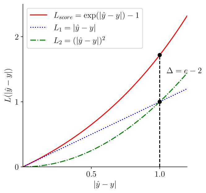
Figure 3: Comparison of the proposed $L_{score}$ and $L_{1}$, $L_{2}$ loss. When the absolute error between the ground-truth and predicted score reaches 1, $L_{score}$ is $e-2$ larger than $L_{1}$ or $L_{2}$ loss, thus refining the score prediction more vigorously.

The score regression loss $L_{score}$ is then defined in Eq. (10). It is a combination of $\text{e}^{v}-1$ and $L_{1}$ loss, which is inspired by an important equivalent infinitesimal $\text{e}^{v}-1\sim v(v\to 0)$. Thus, $v$ is replaced by $\text{e}^{v}-1$. As shown in Fig. 3, due to the property of exponential explosion, $L_{score}$ is much more sensitive to the difference between $\hat{y}$ and $y$ than $L_{1}$ or $L_{2}$ loss. The experiments also demonstrate such superiority.

$$L_{score}=\sum_{i=1}^{n}[\exp(|\hat{y}^{(i)}-y^{(i)}|)-1]$$ (10)

IV-B4 Joint Loss

The learning goal of our framework is to find the parameters through joint learning of attractiveness distribution, rating distribution and score regression, so as to minimize the joint loss $L$.

$$L=\lambda_{1}L_{ad}+\lambda_{2}L_{rd}+\lambda_{3}L_{score}$$ (11)

where $\lambda_{1}$, $\lambda_{2}$ and $\lambda_{3}$ are weights balancing the significance among three types of losses.

Ablation studies with various combinations of $\lambda_{i}=\{1,2,5,10\}(i=1,2,3)$ have been performed. Intuitively, we expect the model with higher-weighted $\lambda_{3}$ would have better performance because our task is to predict the attractiveness score, and the model should focus more on the score regression module. Surprisingly and coincidentally, the model with weights all set to 1 has the best overall performance, thereby $\lambda_{1}=\lambda_{2}=\lambda_{3}=1$ in our experiments.

V Experiments

In this section, we present the experiments to validate the effectiveness of the proposed approach on two benchmark datasets. The implementation details, and comparisons with state-of-the-arts are thoroughly analyzed. Afterwards, extensive ablation studies and visualization are carried out to further demonstrate the superiority of our approach.

V-A Implementation Details

All the experiments are conducted on the popular deep learning framework Pytorch [45] with an NVIDIA Tesla V100 GPU. To ensure the effectiveness, five-folds cross validation is performed, and the average results are reported.

Datasets

The SCUT-FBP5500 [46] and SCUT-FBP [33] datasets are used in our experiments. During the development of these datasets, volunteers were asked to rate the images with integers ranging from 1 to 5, where the score 5 indicates the most attractive. Each image was then labeled with its average score. The full rating records are also provided, allowing us to construct different label distributions.

Data Preprocessing

Since the image size of SCUT-FBP dataset varies, we adopt multi-task cascaded CNN (MTCNN) [47] for face and facial landmark detection. Then, the faces are aligned to upright based on the detected landmarks and resized to 350$\times$350. No preprocessing has been made on SCUT-FBP5500 dataset. Finally, the images of SCUT-FBP5500 are resized to 256$\times$256 and center-cropped to 224$\times$224, while the aligned images of SCUT-FBP are resized to 224$\times$224 directly. Before feeding into the network, all resized images are normalized using the mean and standard deviation of the ImageNet dataset [48] for each color channel.

Data Augmentation

We only perform random horizontal flip with the probability $p=0.5$ in the training phase. No data augmentation has been performed during inference stage.

Training Details

We utilize the ImageNet-pretrained model to initialize the network. Then, the number of output channels of the fully-connected layer in the classifier module, is modified to 40. The network is optimized by AdamW [49], with $\beta=(0.9,0.999)$ and $\epsilon=10^{-8}$. The initial learning rate is 0.001, and it is decreased by a factor of 10 every 30 epochs. Each model is trained 90 epochs with a batch size of 256.

Inference Details

During inference phase, the preprocessed images are fed into the network for evaluation of our approach.

Evaluation Metrics

FAP can be formulated as a regression problem. Hence, the Pearson correlation coefficient (PC), mean absolute error (MAE), and root mean squared error (RMSE) are employed to evaluate the performance of our method, whose formulas are presented in Eq. (12). A higher PC, lower MAE and RMSE suggests better performance. Besides, the model efficiency is measured by the number of parameters and MAdds [18].

$$\text{PC}=\frac{\sum_{i=1}^{N}(y^{(i)}-\bar{y})(\hat{y}^{(i)}-\bar{\hat{y}})}{\sqrt{\sum_{i=1}^{N}(y^{(i)}-\bar{y})^{2}}\sqrt{\sum_{i=1}^{N}(\hat{y}^{(i)}-\bar{\hat{y}})^{2}}}$$ (12)

$$\text{MAE}=\frac{1}{N}\sum_{i=1}^{N}|\hat{y}^{(i)}-y^{(i)}|$$

$$\text{RMSE}=\sqrt{\frac{1}{N}\sum_{i=1}^{N}(\hat{y}^{(i)}-y^{(i)})^{2}}$$

where $N$ denotes the number of images in test set, $\bar{y}=\frac{1}{N}\sum_{i=1}^{N}y^{(i)}$, and $\bar{\hat{y}}=\frac{1}{N}\sum_{i=1}^{N}\hat{y}^{(i)}$.

V-B Comparison with the State of the Art

TABLE II: Comparison with the state of the art on SCUT-FBP5500 and SCUT-FBP datasets. The best results are presented in bold.

Method on SCUT-FBP5500 dataset	Backbone	#Params(M)	MAdds(G)	PC$\uparrow$	MAE$\downarrow$	RMSE$\downarrow$
AaNet [15]	ResNet-18	11.69	1.82	0.9055	0.2236	0.2954
Co-attention learning [25]	MobileNetV2$\times 2$	7.00	0.62	0.9260	0.2020	0.2660
MT-ResNet[39]	ResNet-50	25.56	4.11	0.8905	0.2459	0.3208
R3CNN [14]	ResNeXt-50	25.03	4.26	0.9142	0.2120	0.2800
CNN-ER [37]	Ensemble of 6 models	255.00	-	0.9250	0.2009	0.2650
Ours	MobileNetV2	2.28	0.31	0.9276	0.1964	0.2585
Method on SCUT-FBP dataset	Backbone	#Params(M)	MAdds(G)	PC$\uparrow$	MAE$\downarrow$	RMSE$\downarrow$
LDL [26]	ResNet-50	25.56	4.11	0.9301	0.2127	0.2781
P-AaNet [15]	ResNet-18	11.69	1.82	0.9103	0.2224	0.2816
DLDL-v2 [42]	ThinAttNet	3.69	3.86	0.9300	0.2120	0.2730
R3CNN [14]	ResNeXt-50	25.03	4.26	0.9500	0.2314	0.2885
Ours	MobileNetV2	2.28	0.31	0.9309	0.2212	0.2822

We compare our approach against several recent and representative works on both datasets. The comparison with state of the art is given in Table II, which proves our advantages in terms of performance and efficiency.

High performance

In the SCUT-FBP5500 dataset, our approach achieves state-of-the-art performance on three evaluation metrics, surpassing previous methods utilizing non-lightweight backbones (e.g. ResNets, ResNeXts) [15, 39, 14] by a large margin. The recently proposed CNN-ER [37] adopted a giant ensemble model with dynamic loss functions to facilitate the prediction, yet our method performs slightly better. Additionally, when compared with the method using the same backbone [25], ours still performs a little better. In the SCUT-FBP dataset, our approach has comparable results. Previous studies tend to adopt complicated data augmentation [26, 15] to seek better performance, while ours abandons such techniques to make it simple and lightweight. As for DLDL-v2 [42], we infer that its superiority largely resulted from pretraining. The ThinAttNet was pretrained on the MS-Celeb-1M dataset, a face recognition dataset, which is more relevant to our task than the object classification dataset, e.g. the ImageNet dataset. Compared with the most recent R³CNN [14], although our approach has slightly lower PC, its relatively higher MAE and RMSE indicates poorer predictions, which is unacceptable in FAP.

High efficiency

Our approach has the least parameters and MAdds among the compared methods. Specifically, it is also an extension of our previous work [26], enjoying significantly improved model efficiency while achieving similar performance on SCUT-FBP. Compared with those using ResNet-18 or ResNet-50/ResNeXt-50, our method has 80% or 90% reduction in the number of parameters and MAdds, respectively. A majority of previous methods employ giant models to accomplish better performance. We, however, focus on the lightweight design to enable the model suitable for resource-constrained circumstances.

Overall, our approach succeeds in striking a balance between performance and efficiency, achieving state-of-the-art or comparable results in both datasets while decreasing the number of parameters and MAdds sharply.

V-C Ablation Study

In order to investigate the effectiveness of each learning module and the backbone more precisely, we conduct extensive ablation study in the following.

V-C1 Different combinations of learning modules

TABLE III: Comparison of different combinations of learning modules, where AD, RD, and SR stand for the attractiveness distribution learning module, rating distribution learning module, and score regression learning module, respectively.

Learning module	SCUT-FBP5500			SCUT-FBP
	PC$\uparrow$	MAE$\downarrow$	RMSE$\downarrow$	PC$\uparrow$	MAE$\downarrow$	RMSE$\downarrow$
AD	0.9147	0.5651	0.6823	0.8168	0.6651	0.7902
AD + RD	0.9243	0.2094	0.2746	0.9169	0.2679	0.3301
AD + SR	0.9272	0.1966	0.2592	0.9271	0.2273	0.2900
AD + RD + SR	0.9276	0.1964	0.2585	0.9309	0.2212	0.2822

To demonstrate all learning modules are indispensable and internally correlated, different combinations of them are compared in Table III. The models with only attractiveness distribution (AD) learning module perform poorly with exceedingly high MAE and RMSE, along with a terribly low PC on SCUT-FBP. After introducing the rating distribution (RD) or score regression (SR) learning module, the performance is significantly improved. It is noteworthy that the introduction of the SR learning module enables the model to perform quite close to the full model, which can be well explained that our task is to predict facial attractiveness in the form of score. Compared with the rating distribution, the attractiveness score is more relevant to our task. Furthermore, the performance continues to grow when we utilize the full model. Such growth is particularly significant on SCUT-FBP, indicating that smaller datasets benefit more from the rating distribution and score regression learning modules.

We can draw some conclusions from the above results. First, all modules are indeed indispensable. The AD learning module is the base, and the other two refine the prediction by introducing related supervised information. To a certain extent, the SR learning module is a must for our task. Second, smaller dataset requires more supervision for better performance, but one should be cautious about the issue of overfitting simultaneously. Finally, appropriate supervision is of vital importance for training. The choice of supervision also matters, which avoids internal redundancy.

V-C2 Different backbones

To explore the efficacy of different backbones, we carry out experiments under the identical settings on some representative backbones, which are categorized as traditional or lightweight. As shown in Table IV, MobileNetV2 has the best overall performance on both datasets, especially on SCUT-FBP, surpassing other backbones by a large margin. As for traditional backbones, ResNet-18 has similar results but the parameters and MAdds boost 5 times. All evaluation metrics suffer when using deeper variants of ResNet or VGG, notably in SCUT-FBP. We infer that such phenomenon mainly results from overfitting and overtraining. First, there are only 4400 and 400 training samples in the datasets, respectively. Training a giant model (e.g. ResNet-50) with a small or tiny dataset is prone to overfit. Second, we notice that models with ResNet-50 or VGG19 have larger training loss than the corresponding ResNet-18 or VGG16, suggesting that the training settings might not suitable for the deeper architectures. Lastly, we adjust the training setup of ResNet-50 model to have it properly trained and indeed obtain improved performance, whereas it is still inferior to the model employing MobileNetV2.

As for lightweight backbones, we conduct experiments on MobileNetV3 [19]. The formerly proposed MobileNetV2 still enjoys clear superiority. We notice that the performance declines with larger MobileNetV3 on SCUT-FBP, which is consistent with the traditional backbones. Thus, we can conclude that the choice of backbone in terms of scale and structure is of significance to performance and requires careful consideration.

TABLE IV: Comparison of different backbones.

Backbone	#Params(M)	MAdds(G)	SCUT-FBP5500			SCUT-FBP
			PC$\uparrow$	MAE$\downarrow$	RMSE$\downarrow$	PC$\uparrow$	MAE$\downarrow$	RMSE$\downarrow$
ResNet-18	11.20	1.82	0.9262	0.1961	0.2605	0.9238	0.2295	0.3007
ResNet-50	23.59	4.11	0.9198	0.2058	0.2728	0.9067	0.2591	0.3354
VGG16	14.74	15.39	0.9267	0.1952	0.2593	0.9164	0.2627	0.3377
VGG19	20.06	19.55	0.9251	0.1978	0.2621	0.9135	0.2719	0.3515
MobileNetV3_large	4.25	0.22	0.9210	0.2025	0.2688	0.9122	0.2776	0.3472
MobileNetV3_small	1.56	0.06	0.9103	0.2142	0.2850	0.9156	0.2631	0.3427
MobileNetV2	2.28	0.31	0.9276	0.1964	0.2585	0.9309	0.2212	0.2822

V-C3 Different label distribution learning schemes

To demonstrate the superiority of our approach among LDL methods, we carry out the following comparative experiments. The approach in [26] is reimplemented on SCUT-FBP5500, since the dataset had not been released at the published time of the paper. Then, the method in [28], which was originally designed for age estimation, was adapted to FAP for being a similar regression task in [42]. For fair comparison, the methods mentioned above are reimplemented using MobileNetV2 under identical training settings. Furthermore, we compare the performance of Gaussian and Laplace distribution by replacing the probability distribution employed in the attractiveness distribution. As shown in Table V, our delicately designed approach achieves the best performance on both datasets, notably in SCUT-FBP, outperforming other methods greatly. When comparing Laplace and Gaussian distribution, our approach with Laplace distribution performs slightly better on SCUT-FBP5500, but has a significant improvement on SCUT-FBP, proving the effectiveness and simplicity of Laplace distribution.

TABLE V: Comparison of different LDL schemes.

LDL scheme	SCUT-FBP5500			SCUT-FBP
	PC$\uparrow$	MAE$\downarrow$	RMSE$\downarrow$	PC$\uparrow$	MAE$\downarrow$	RMSE$\downarrow$
[26]	0.9259	0.1965	0.2606	0.9211	0.2283	0.2954
[28, 42]	0.9253	0.2074	0.2722	0.9184	0.2692	0.3439
Ours with Gaussian distribution	0.9275	0.1966	0.2587	0.9263	0.2271	0.2910
Ours with Laplace distribution	0.9276	0.1964	0.2585	0.9309	0.2212	0.2822

V-D Visualization

To better understand how our model perceive the abstract facial attractiveness, we visualize a feature map, which can intuitively present the prediction patterns of different degrees of attractiveness, and indicate the reasons of good or poor predictions.

The ReLU6 activation layer in the last convolution block of MobileNetV2 produces 7$\times$7 feature maps with 1280 channels. These feature maps are first channel-wise averaged and resized to 224$\times$224. Then, as shown in Fig. 4, heatmap visualization is conducted and covered on the input images.

From good predictions, it can be concluded that with increasing degree of attractiveness, our approach gradually focuses on certain facial regions (e.g., mouth, eyes, nose) and produces semantic predictions. In Fig. 4(a), the high intensity areas almost cover the whole face, indicating that the model fails to locate attractive facial regions, resulting in a relatively low attractiveness score. In Fig. 4(b)(c), the high intensity areas gradually narrow down to smaller areas, presenting ambiguously semantic predictions. Specifically, when the face is attractive, the model is able to capture the abstract facial attractiveness, concentrating on facial regions with evident semantics, such as eyes and nose in Fig. 4(d). From poor predictions, we notice that our approach mainly focus on the irrelevant regions, such as hair, regions outside face, and background, leading to failure in capturing attractiveness, as shown in Fig. 4(e)-(h).

To sum up, our approach is capable of sensing facial beauty and capturing attractive facial regions to accomplish accurate and efficient FAP. However, it still has some limitations, mainly due to focusing on the irrelevant areas of the images.

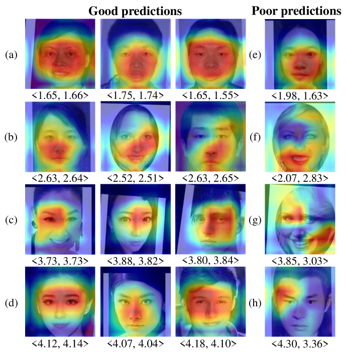
Figure 4: The heatmap visualization, where warmer colors (e.g., red) indicate higher intensity and cooler colors (e.g., blue) indicate lower intensity. Each row comes from a distinct degree of attractiveness. The left three columns ((a)-(d)) and the rightmost column ((e)-(h)) are examples of good and poor predictions, respectively. The pairs below the images stand for $<$ground-truth score, predicted score$>$.

VI Conclusion

In this paper, we integrate the lightweight design and LDL paradigm to develop a novel facial attractiveness prediction model, which consists of: (1) the dual label distribution to take full advantage of the dataset; (2) a joint learning framework to optimize the dual label distribution and attractiveness score simultaneously. The proposed approach achieves appealing results with greatly decreased parameters and computation. The visualization demonstrates that our approach is interpretable, employing different patterns to capture facial attractiveness so as to generate semantic predictions.

However, our work remains multiple interesting yet undiscovered directions for future explorations. First, the proposed dual label distribution is expected to generalize to other similar tasks, such as age prediction and facial expression recognition. For datasets without sufficient information, pseudo distribution can be generated to employ our dual label distribution learning paradigm. Second, our work is based on static images, which fails to take temporal cues into consideration. In fact, psychological [50] and neuroscience [51] studies have proven that temporal cues play a vital role in perceiving facial attractiveness. Nevertheless, little attention has paid to dynamic facial contents, and the temporal dynamics of facial attractiveness remains largely unexplored. Kalaycı et al. [52] utilized dynamic and static features extracted from video clips for facial attractiveness analysis. Recently, Weng et al. [53] conducted dynamic facial attractiveness prediction utilizing videos from TikTok. Third, only frontal facial images are employed in our work, which cannot well reflect facial structure and lack variations in visual angles. Researchers have shown that facial attractiveness is jointly determined by frontal view, profile view, and their combination [54]. Therefore, adopting multi-view or three-dimensional facial data for facial attractiveness analysis and prediction is of significance, which is expected to produce more comprehensive and reliable results, and thus better reveal the secrets of facial attractiveness. However, such direction has received little attention, and it was until recent years that some researchers started to investigate [55, 56, 57].

References

- [1] M. Bashour, “History and current concepts in the analysis of facial attractiveness,” Plastic and Reconstructive Surgery, vol. 118, no. 3, pp. 741–756, 2006.
- [2] G. Rhodes and J. Haxby, The Oxford handbook of face perception. Oxford University Press, 2011.
- [3] S. Liu, Y.-Y. Fan, A. Samal et al., “Advances in computational facial attractiveness methods,” Multimedia Tools and Applications, vol. 75, no. 23, pp. 16 633–16 663, 2016.
- [4] J. Li, C. Xiong, L. Liu et al., “Deep face beautification,” in ACM International Conference on Multimedia, 2015, pp. 793–794.
- [5] L. Liang, L. Jin, and D. Liu, “Edge-aware label propagation for mobile facial enhancement on the cloud,” IEEE Transactions on Circuits and Systems for Video Technology, vol. 27, no. 1, pp. 125–138, 2017.
- [6] N. Sun, J. Tao, J. Liu, H. Sun, and G. Han, “3d facial feature reconstruction and learning network for facial expression recognition in the wild,” IEEE Transactions on Cognitive and Developmental Systems, 2022.
- [7] R. Rothe, R. Timofte, and L. Van Gool, “Some like it hot-visual guidance for preference prediction,” in IEEE Conference on Computer Vision and Pattern Recognition, 2016, pp. 5553–5561.
- [8] A. Bottino, M. De Simone, A. Laurentini et al., “A new 3-d tool for planning plastic surgery,” IEEE Transactions on Biomedical Engineering, vol. 59, no. 12, pp. 3439–3449, 2012.
- [9] P. Aarabi, D. Hughes, K. Mohajer et al., “The automatic measurement of facial beauty,” in IEEE International Conference on Systems, Man and Cybernetics, vol. 4, 2001, pp. 2644–2647.
- [10] F. Chen and D. Zhang, “Combining a causal effect criterion for evaluation of facial attractiveness models,” Neurocomputing, vol. 177, pp. 98–109, 2016.
- [11] A. Kagian, G. Dror, T. Leyvand et al., “A humanlike predictor of facial attractiveness,” in International Conference on Neural Information Processing Systems, 2006, pp. 649–656.
- [12] D. Zhang, F. Chen, Y. Xu et al., Computer models for facial beauty analysis. Springer, 2016.
- [13] D. Gray, K. Yu, W. Xu et al., “Predicting facial beauty without landmarks,” in European Conference on Computer Vision, 2010, pp. 434–447.
- [14] L. Lin, L. Liang, and L. Jin, “Regression guided by relative ranking using convolutional neural network (r3cnn) for facial beauty prediction,” IEEE Transactions on Affective Computing, vol. 13, no. 1, pp. 122–134, 2022.
- [15] L. Lin, L. Liang, L. Jin et al., “Attribute-aware convolutional neural networks for facial beauty prediction.” in International Joint Conference on Artificial Intelligence, 2019, pp. 847–853.
- [16] F. N. Iandola, S. Han, M. W. Moskewicz et al., “Squeezenet: Alexnet-level accuracy with 50x fewer parameters and 0.5 mb model size,” arXiv preprint arXiv:1602.07360, 2016.
- [17] A. G. Howard, M. Zhu, B. Chen et al., “Mobilenets: Efficient convolutional neural networks for mobile vision applications,” arXiv preprint arXiv:1704.04861, 2017.
- [18] M. Sandler, A. Howard, M. Zhu et al., “Mobilenetv2: Inverted residuals and linear bottlenecks,” in IEEE Conference on Computer Vision and Pattern Recognition, 2018, pp. 4510–4520.
- [19] A. Howard, M. Sandler, G. Chu et al., “Searching for mobilenetv3,” in IEEE/CVF International Conference on Computer Vision, 2019, pp. 1314–1324.
- [20] D. Zhou, Q. Hou, Y. Chen, J. Feng, and S. Yan, “Rethinking bottleneck structure for efficient mobile network design,” in European Conference on Computer Vision, 2020, pp. 680–697.
- [21] M. Tan and Q. Le, “Efficientnet: Rethinking model scaling for convolutional neural networks,” in International Conference on Machine Learning, 2019, pp. 6105–6114.
- [22] Q. Xie, M.-T. Luong, E. Hovy et al., “Self-training with noisy student improves imagenet classification,” in IEEE/CVF Conference on Computer Vision and Pattern Recognition, 2020, pp. 10 687–10 698.
- [23] C. Xie, M. Tan, B. Gong et al., “Adversarial examples improve image recognition,” in IEEE/CVF Conference on Computer Vision and Pattern Recognition, 2020, pp. 819–828.
- [24] M. Tan, R. Pang, and Q. V. Le, “Efficientdet: Scalable and efficient object detection,” in IEEE/CVF Conference on Computer Vision and Pattern Recognition, 2020, pp. 10 781–10 790.
- [25] S. Shi, F. Gao, X. Meng et al., “Improving facial attractiveness prediction via co-attention learning,” in IEEE International Conference on Acoustics, Speech and Signal Processing, 2019, pp. 4045–4049.
- [26] Y.-Y. Fan, S. Liu, B. Li et al., “Label distribution-based facial attractiveness computation by deep residual learning,” IEEE Transactions on Multimedia, vol. 20, no. 8, pp. 2196–2208, 2018.
- [27] X. Geng, “Label distribution learning,” IEEE Transactions on Knowledge and Data Engineering, vol. 28, no. 7, pp. 1734–1748, 2016.
- [28] B.-B. Gao, H.-Y. Zhou, J. Wu et al., “Age estimation using expectation of label distribution learning,” in International Joint Conference on Artificial Intelligence, 2018, pp. 712–718.
- [29] Y. Zhou, H. Xue, and X. Geng, “Emotion distribution recognition from facial expressions,” in ACM International Conference on Multimedia, 2015, pp. 1247–1250.
- [30] K. Su and X. Geng, “Soft facial landmark detection by label distribution learning,” in AAAI Conference on Artificial Intelligence, vol. 33, 2019, pp. 5008–5015.
- [31] A. Krizhevsky, I. Sutskever, and G. E. Hinton, “Imagenet classification with deep convolutional neural networks,” Advances in neural information processing systems, vol. 25, 2012.
- [32] O. M. Parkhi, A. Vedaldi, and A. Zisserman, “Deep face recognition,” in British Machine Vision Conference, 2015.
- [33] D. Xie, L. Liang, L. Jin et al., “Scut-fbp: A benchmark dataset for facial beauty perception,” in IEEE International Conference on Systems, Man, and Cybernetics, 2015, pp. 1821–1826.
- [34] K. Simonyan and A. Zisserman, “Very deep convolutional networks for large-scale image recognition,” arXiv preprint arXiv:1409.1556, 2014.
- [35] L. Xu, J. Xiang, and X. Yuan, “Transferring rich deep features for facial beauty prediction,” arXiv preprint arXiv:1803.07253, 2018.
- [36] J. Xu, L. Jin, L. Liang, Z. Feng, D. Xie, and H. Mao, “Facial attractiveness prediction using psychologically inspired convolutional neural network (pi-cnn),” in IEEE International Conference on Acoustics, Speech and Signal Processing, 2017, pp. 1657–1661.
- [37] F. Bougourzi, F. Dornaika, and A. Taleb-Ahmed, “Deep learning based face beauty prediction via dynamic robust losses and ensemble regression,” Knowledge-Based Systems, vol. 242, p. 108246, 2022.
- [38] L. Xu, H. Fan, and J. Xiang, “Hierarchical multi-task network for race, gender and facial attractiveness recognition,” in IEEE International Conference on Image Processing, 2019, pp. 3861–3865.
- [39] J. Xu, “Mt-resnet: a multi-task deep network for facial attractiveness prediction,” in IEEE 2nd International Conference on Computing and Data Science, 2021, pp. 44–48.
- [40] Y.-F. Song, Z. Zhang, C. Shan, and L. Wang, “Constructing stronger and faster baselines for skeleton-based action recognition,” IEEE Transactions on Pattern Analysis and Machine Intelligence, 2022.
- [41] X. Sun, C. Chen, X. Wang, J. Dong, H. Zhou, and S. Chen, “Gaussian dynamic convolution for efficient single-image segmentation,” IEEE Transactions on Circuits and Systems for Video Technology, vol. 32, no. 5, pp. 2937–2948, 2022.
- [42] B.-B. Gao, X.-X. Liu, H.-Y. Zhou, J. Wu, and X. Geng, “Learning expectation of label distribution for facial age and attractiveness estimation,” arXiv preprint arXiv:2007.01771v2, 2021.
- [43] Y. Ren and X. Geng, “Sense beauty by label distribution learning,” in International Joint Conference on Artificial Intelligence, 2017, pp. 2648–2654.
- [44] L. Chen and W. Deng, “Facial attractiveness prediction by deep adaptive label distribution learning,” in Chinese Conference on Biometric Recognition, 2019, pp. 198–206.
- [45] A. Paszke, S. Gross, F. Massa et al., “Pytorch: An imperative style, high-performance deep learning library,” in International Conference on Neural Information Processing Systems, 2019, pp. 8026–8037.
- [46] L. Liang, L. Lin, L. Jin et al., “Scut-fbp5500: A diverse benchmark dataset for multi-paradigm facial beauty prediction,” in International Conference on Pattern Recognition, 2018, pp. 1598–1603.
- [47] K. Zhang, Z. Zhang, Z. Li et al., “Joint face detection and alignment using multitask cascaded convolutional networks,” IEEE Signal Processing Letters, vol. 23, no. 10, pp. 1499–1503, 2016.
- [48] J. Deng, W. Dong, R. Socher et al., “Imagenet: A large-scale hierarchical image database,” in IEEE Conference on Computer Vision and Pattern Recognition, 2009, pp. 248–255.
- [49] I. Loshchilov and F. Hutter, “Decoupled weight decay regularization,” in International Conference on Learning Representations, 2019.
- [50] A. J. Rubenstein, “Variation in perceived attractiveness: Differences between dynamic and static faces,” Psychological science, vol. 16, no. 10, pp. 759–762, 2005.
- [51] A. J. O’Toole, D. A. Roark, and H. Abdi, “Recognizing moving faces: A psychological and neural synthesis,” Trends in cognitive sciences, vol. 6, no. 6, pp. 261–266, 2002.
- [52] S. Kalayci, H. K. Ekenel, and H. Gunes, “Automatic analysis of facial attractiveness from video,” in IEEE International Conference on Image Processing, 2014, pp. 4191–4195.
- [53] N. Weng, J. Wang, A. Li, and Y. Wang, “Two-stream temporal convolutional network for dynamic facial attractiveness prediction,” in International Conference on Pattern Recognition, 2021, pp. 10 026–10 033.
- [54] Q. Liao, X. Jin, and W. Zeng, “Enhancing the symmetry and proportion of 3d face geometry,” IEEE transactions on visualization and computer graphics, vol. 18, no. 10, pp. 1704–1716, 2012.
- [55] S. Liu, Y. Fan, Z. Guo, and A. Samal, “2.5 d facial attractiveness computation based on data-driven geometric ratios,” in International Conference on Intelligent Science and Big Data Engineering, 2015, pp. 564–573.
- [56] S. Liu, Y.-Y. Fan, Z. Guo, A. Samal, and A. Ali, “A landmark-based data-driven approach on 2.5 d facial attractiveness computation,” Neurocomputing, vol. 238, pp. 168–178, 2017.
- [57] Q. Xiao, Y. Wu, D. Wang, Y.-L. Yang, and X. Jin, “Beauty3dfacenet: deep geometry and texture fusion for 3d facial attractiveness prediction,” Computers & Graphics, vol. 98, pp. 11–18, 2021.