ISAC-Enabled Beam Alignment for Terahertz Networks: Scheme Design and Coverage Analysis

Abstract

As a key pillar technology for the future 6G networks, terahertz (THz) communication can provide high-capacity transmissions, but suffers from severe propagation loss and line-of-sight (LoS) blockage that limits the network coverage. Narrow beams are required to compensate for the loss, but they in turn bring in beam misalignment challenge that degrades the THz network performance. The high sensing accuracy of THz signals enables integrated sensing and communication (ISAC) technology to assist the LoS blockage and user mobility-induced beam misalignment, enhancing THz network coverage. In line with the 5G beam management, we propose a joint synchronization signal block (SSB) and reference signal (RS)-based sensing (JSRS) scheme to predict the need for beam switches, and thus prevent beam misalignment. We further design an optimal sensing signal pattern that minimizes beam misalignment with fixed sensing resources, which reveals design insights into the time-to-frequency allocation. We derive expressions for the coverage probability and spatial throughput, which provide instructions on the ISAC-THz network deployment and further enable evaluations for the sensing benefit in THz networks. Numerical results show that the JSRS scheme is effective and highly compatible with the 5G air interface. Averaged in tested urban use cases, JSRS achieves near-ideal performance and reduces around $80\%$ of beam misalignment, and enhances the coverage probability by about $75\%$, compared to the network with 5G-required positioning ability.

I Introduction

Towards the realization of smart cities, the future 6G foresees the implementation of authentic digital twin representation of the physical world, supporting novel use cases, including but not limited to vehicle-to-everything (V2X) communications, unmanned air vehicles (UAV) and smart factories[1]. The ultra-wide terahertz (THz) band that can support massive connections with up to terabit per second (Tbps) data rate has come into vision[2].

However, THz-band transmissions suffer from limited signal power, high propagation loss and severe molecular absorption, causing the coverage bottleneck[3]. Highly directional beams are exploited to enhance the signal power, but they bring in narrow beam alignment challenges[4]. Furthermore, the THz link is sensitive to line-of-sight (LoS) blockage, meaning objects larger than several wavelengths can interrupt the connection[5, 6]. Frequent beam switches and severe beam misalignment cause link interruption and non-negligible latency for link reconstruction, which severely degrades the communication quality, including the coverage probability and throughput[7, 8]. Thus, it is essential to develop an efficient beam alignment scheme for THz networks [9, 10].

Sensing has been exploited for high-precise positioning, which has the potential to be used to provide assistance for beam alignment[11]. The ultra-high THz signals intrinsic high-resolution sensing, opening up unprecedented opportunities to realize integrated sensing and communication (ISAC) in THz networks[12]. It allows for joint sensing and communication using unified waveform and integrated hardware[13]. Compared to the traditional sensor-aided solutions, ISAC uses shared resources that can achieve low latency and high spectral efficiency with reduced cost[14]. The state-of-the-art THz band ISAC prototypes have realized millimetre-level imaging resolution, showing its feasibility to assist THz communications[15]. However, from the ISAC prototype to the implementation of sensing-aided THz communications, the following challenges need to be addressed: 1) The design of a sensing-aided beam alignment scheme that is compatible with the current 5G beam management procedure; 2) The flexible sensing signal configuration that efficiently uses the sensing resources in varying networks; 3) Network-level performance analysis that captures the enhancement provided by the sensing assistance.

To tackle the aforementioned challenges, many foundational works have contributed to the link-level ISAC-THz techniques. Work[16, 17, 18, 19, 20] focus on sensing information extraction and ISAC waveform design. For candidate standard signal selection, the standard signals are preferred to be sensing candidates to realize better compatibility with the 5G air interface. Theoretically, work[21] compares the feasibility of using the channel estimation signals, synchronization signal block (SSB), demodulation reference signals (DMRS) and positioning reference signals (PRS) for sensing. As pilot signals, they shine with intrinsic auto-correlation and anti-noise properties that improve localization accuracy[22]. Work[23] develops RS-based angle and time estimation algorithms and evaluates the superiority of using reference signals (RSs) over other standard signals for localization in V2X networks. Work[22] provides frame structure design for PRS-based sensing signal configuration to perform velocity estimation. However, the sensing-aided communication scheme that benefits network-level performance has not been well investigated.

Till now, few works have been done to bridge the gap from the link level to the network level, covering areas from the scheme design, sensing signal configuration to performance evaluation. As a preliminary discussion on the scheme design, our previous work[24] proposes an SSB-based sensing method to assist the THz/mmWave network beam alignment. However, its benefits on network coverage and throughput have not been analysed. Considering the cost and benefit of sensing, work [25] designs a networking-based ISAC hardware testbed that reveals the resource allocation trade-off between communication and sensing functions. However, it does not provide an effective scheme to configure the sensing signals, and no sensing-aided communication scheme has been considered.

For network performance analysis, stochastic geometry (SG) is a well-investigated tool that has been widely used to model networks ranging up to THz bands. Key performance indicators ranging from interference, coverage probability to spatial throughput can be modelled using the basic theories developed in [26, 27, 28]. The interference and coverage probability is discussed in works[29, 30], and the spatial throughput and spectral efficiency are analysed in[31, 32]. Recently, SG has also been exploited for ISAC network modelling. Work[33] analyses the maximum radar detection range and throughput for the coexisting ISAC network. Work[32] develops a mathematical framework that characterizes the coverage and ergodic capacity of ISAC-based networks, but the coverage enhancement by introducing sensing into the system has not been analysed. Moreover, these works for ISAC are for mmWave and below bands. For the THz network with ISAC, the unique THz propagation features, LoS blockage and mobility effects need to be considered. There still remain blanks for the analysis on the ISAC benefit in THz network coverage and throughput.

To solve the beam misalignment challenge in THz networks, from the network level, we propose an ISAC-based beam alignment approach that enhances the network coverage, which is in line with the 5G standard. The main contributions are summarised as follows.

1) We propose a joint SSB and RS-based sensing (JSRS) scheme to reduce the LoS blockage and user mobility-induced beam misalignment in THz networks, which is in line with the 5G beam management procedure. JSRS exploits the 5G-specified SSBs to detect blockages and the RSs for user tracking. Different from the traditional detect-and-correct method, sensing-based JSRS enables a predict-and-prevent procedure that provides early interventions for timely beam switches, avoiding beam misalignment.

2) Based on the 5G frame structure, we provide an optimal sensing signal pattern design which minimizes beam misalignment with a given number of sensing resources. Specifically, we optimize the time-to-frequency allocation ratio that minimises the sensing error-induced beam misalignment, and the insert spacings to satisfy the sensing range and resolution requirements. We reveal the design trade-offs in the time-to-frequency allocation ratio affected by the beamwidth and frequency bands (see Theorem 1).

3) From the network level, we then provide expressions for the coverage probability and spatial throughput based on stochastic geometry. They enable evaluations on the benefit of introducing sensing into THz networks and provide instructions for the ISAC-THz network deployment that achieves wider coverage and higher spatial throughput, including the design of network density, beamwidth and sensing signal configuration (see Theorem 2).

4) Based on the numerical analyses, we show the effectiveness of the JSRS scheme and its high compatibility with the 5G air interface. In tested urban V2X use cases, the JSRS scheme averagely reduces the beam misalignment by $80\%$, increasing the coverage probability by $75\%$, compared to that of the 5G-ability networks. Besides, the JSRS scheme achieves near-ideal performance, showing that the proposed sensing signal configuration effectively reduces the estimation error. JSRS exploited the high angular resolution of narrow beams to enhance the distance estimation, and thus turn the disadvantage of sharp beams into benefits, allowing the THz network to use narrower beams to enhance coverage and throughput.

The remainder of this paper is organized as follows. Sec.II introduces the ISAC-THz network model and the challenge of THz beam alignment. Sec.III proposes the JSRS scheme for THz beam alignment and analyses its feasibility. Sec.IV provides a time-frequency sensing signal pattern design and evaluates the cost of sensing. The analytical coverage probability and throughput expressions for the ISAC-THz network are given in Sec.V. Numerical results are presented in Sec.VI. Conclusions are drawn in Sec.VII. The definitions of frequently used symbols are summarized in Table I.

II System Model

In this section, we first give the THz signal propagation and noise models, and then depict the stochastic geometry-based ISAC-THz network deployment. Considering the 5G-specified beam management procedure, we then emphasize on the narrow beam misalignment challenge in the THz network.

TABLE I: Symbols definition.

Symbol	Definition
$r_{\rm{B}}$	Node radius
$\lambda_{B},\lambda_{M},\lambda_{S}$	Densities of BSs, MTs, and blockers
$n_{b/m}$	BS/MT beam number
$\theta_{b/m}$	The beamwidth at BS/MT
$\mu_{g}$	The density of beam switch points
$K$	Molecular absorption coefficient
$P_{\rm{C}}$	Transmit signal power
$P_{\rm{N}}^{\rm{T}},P_{\rm{N}}^{\rm{M}},P_{\rm{N}}$	The thermal, molecular absorption and total noise
$f_{c}$	Central frequency
$f_{\rm{scs}}$	Subcarrier spacing
$T_{\rm{sym}}$	Symbol length
$\tau$	SSB period
$U,V$	Frequency, time-domain spacing
$N_{\rm{RS}},N_{\rm{SSB}}$	Number of REs for RSs and SSBs
$N_{s},N_{f}$	Number of REs in time and frequency domain
$\alpha$	Time-frequency allocation ratio
$B_{\rm{S}},T_{\rm{S}}$	The RS bandwidth and time duration
$B_{\rm{SSB}},T_{\rm{SSB}}$	The SSB bandwidth and time duration
$\Delta r,\Delta d_{b},\Delta v$	The distance, motion and velocity resolutions
$d_{\rm{max}},v_{\rm{max}}$	The unambiguous range and velocity
$r_{1},r_{2},r_{i}$	Distance to the closest, 2${}^{\rm{nd}}\!$ close and interfering BSs
$p_{\rm{m}}^{\rm{s}}$	Beam misalignment probability
$p_{\rm{B}}^{r_{1}},p_{\rm{B}}^{r_{2}}$	Blocked probability of the closet and 2nd close BSs
$p_{\rm{B}}^{to}$	Timeout probability
$p_{\rm{I}}$	The BS interfere probability
$P_{\rm{UB}}^{I}$	Unblocked probability of the interferer
$\mathcal{T}$	SINR threshold
$p_{\rm{cvp}}$	The coverage probability
$\beta$	The ratio of sensing cost to total REs
$\!\tau_{\rm{thr}},d_{\rm{thr}},\eta_{\rm{SE}}$	Link throughput, spatial throughput, spectral efficiency

II-A THz Signal Propagation Model and Noise Model

In this paper, we adopt a commonly used THz propagation model [3]. The propagation loss is written as

$$L(r,f_{c})=\left({4\pi rf_{c}}/{c}\right)^{2}e^{Kr},$$ (1)

where $r$ is the transmission distance, $c$ is the speed of light, and $K$ is the absorption coefficient depending on the transmission frequency $f_{c}$. The directional antenna gain is modelled using a simplified cone model given as[5]

$$G_{\rm{b/m}}=\frac{2}{1-\cos\left(\frac{1}{2}\theta_{b/m}\right)}.$$ (2)

Combining the path loss and antenna gain, the total received power is written as

$$P_{\rm{C}}(r)\!=\!P_{\rm{T}}G_{b}G_{m}\frac{1}{L(r,f)}\!=\!Ar^{-2}e^{-Kr},$$ (3)

where $\!P_{\rm{T}}\!$ is the transmit power, and $\!A\!=\!P_{\rm{T}}G_{b}G_{m}\!\tfrac{c^{2}}{16\pi^{2}f^{2}}\!$.

Different from low-band networks, the molecular absorption noise at the THz band has a noticeable impact[3]. Induced by the re-radiation of absorbed signal energy, molecular absorption noise depends on the transmit signal power, BS density and beamwidth. Thus, the noise power in the THz network consists of the thermal noise $P_{\rm{N}}^{\rm{T}}$, and the molecular absorption noise $P_{\rm{N}}^{\rm{M}}$[34]. In this paper, we adopt the THz molecular absorption noise model proposed in [35]. The total noise power in THz network is given as

$$P_{\rm{N}}=P_{\rm{N}}^{\rm{T}}+P_{\rm{N}}^{\rm{M}}=P_{\rm{N}}^{\rm{T}}+\sum\nolimits_{i=1}^{{N_{{\rm{BS}}}}}\frac{1}{{{n_{b}}{n_{m}}}}AKr_{i}^{-2}{e^{-K{r_{i}}}},$$ (4)

where $N_{\rm{BS}}$ is the number of BSs in the THz network, and $r_{i}$ is the distance of the $i$-th BS to the typical user.

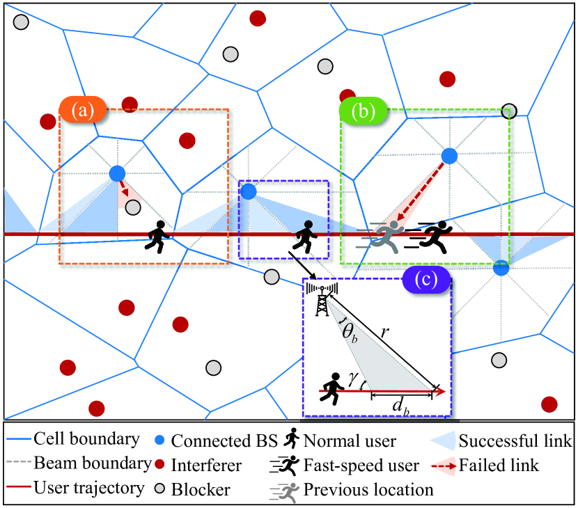
Figure 1: Network deployment, (a) LoS blockage and (b) user mobility-induced beam misalignment. (c) User trajectory.

II-B Network Deployment and Beam Misalignment Problem

We focus on the outdoor applications of the ISAC-THz networks, considering the impact of the macro-scale movement and LoS blockage. Based on the well-developed stochastic geometry, the base stations (BSs), mobile terminals (MTs) and blockers are independently distributed following Poisson point process (PPP) distribution with intensity $\lambda_{B},\lambda_{M},\lambda_{S}$[26]. The nodes are considered as round dots with the same radius $r_{\rm{B}}$. Noticing the LoS-blockage effect at the THz band, the BSs and MTs are also considered as potential blockers. Directional antennas are used at both the BSs and MTs to enhance the signal power. The beam number at the BS and MT sides are $n_{b},n_{m}$, and the corresponding beamwidth are $\theta_{b}=2\pi/(n_{b}),\theta_{m}=2\pi/(n_{m})$ respectively. Considering the widely used maximum receiver power (MRP) scheme, the MT prefers to connect to the closest available BS, forming a Poisson-Voronoi cell tessellation as plotted in Fig.1[28]. The typical MT moves along a randomly oriented straight line with a speed of $v$, drawn by the red line. The beam switch points are the intersections of the beam boundary and user trajectory.

This paper is built based on the 5G-specified beam management procedure. The key tasks include the establishment of suitable beam pair before data transmission, and the beam adjustment to maintain the connection during user movement[36]. Untimely beam switch results in unmatched beam pair on the MT and BS sides, defined as beam misalignment[7]. To handle such beam failures, the 5G new radio (NR) specifies measurement-based beam reselection to recover the beams[36]. The identification of a new candidate beam relies on the measurement of the periodically transmitted SSBs, each of which corresponds to a specific beam and indicates its connectivity. Next, the candidate beam-pair is determined at the BS side based on the SSB measurement reported by the user[7]. Thus, the user needs to receive at least one set of SSBs during current beam coverage for new candidate-beam selection, meaning missed reception of SSBs causes beam misalignment. The following two major causes of beam misalignment are considered in this paper, as plotted in Fig.1.

II-B1 Blockage-Induced Misalignment

As in Fig.1(a), considering the THz LoS-sensitive feature, the blockage on the LoS link causes a blind zone that interrupts the reception of SSBs.

II-B2 Mobility-Induced Misalignment

As in Fig.1(b), since the narrow beamwidth shortens single beam coverage, fast-moving users are unable to receive the scheduled SSBs before reaching the beam boundaries. In other words, the duration within one beam coverage is shorter than the SSB period.

Therefore, an efficient beam alignment scheme in line with 5G-specified beam management is needed. Thanks to the high sensing accuracy of THz signals, sensing can be exploited to assist THz beam alignment.

III Joint SSB and RS-Based Sensing-Aided THz Communication

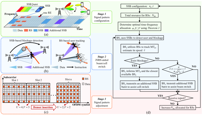
Figure 2: (a) ISAC-frame structure, (b) SSB-based blockage detection and RS-based user tracking, (c) sensing signal configuration and (d) JSRS beam alignment scheme.

In this section, we first introduce the 5G-evolved ISAC-frame structure as a basis. Based on the 5G beam management procedure, we propose a joint SSB and RS-based sensing (JSRS) scheme to assist THz beam alignment. Different from the traditional detect-and-correct error method, the idea of JSRS follows a predict-and-prevent error procedure, that can avoid the occurrence of beam misalignment.

III-A 5G-Evolved ISAC-Frame Structure

To be compatible with the 5G air interface, the ISAC-frame structure is evolved from the 5G that has flexible numerology and the ability to support high-band communications.

One key waveform candidate for ISAC is the current dominant orthogonal frequency division multiplexing (OFDM) waveform, which has excellent multiplexing capability and pilot-bearing symbols[37]. Using OFDM-based transmission, in the time domain, NR transmissions are organized into frames that are divided into slots. One slot consists of $14$ OFDM symbols[36]. In the frequency domain, the resource is divided by subcarriers. Thus, the smallest physical resource defined in 5G NR is resource element (RE) that consists of one subcarrier during one OFDM symbol[36]. Evolved from 5G numerology to support THz communication, we adopt a subcarrier spacing of $f_{\rm{scs}}=1.92{\rm{MHz}}$ and the OFDM symbol length as $T_{\rm{sym}}=4.46\mu{\rm{s}}$, suggested by [38, 39].

The 5G-evolved ISAC-frame structure is plotted in Fig.2(a). According to 3GPP standard[36], one SSB takes up $4$ symbols in time and $240$ subcarriers in frequency, plotted as the blue blocks. The default SSB period is $\tau=20{\rm{ms}}$. NR specifies a beam-swept and time-multiplexed transmission of SSBs. A set of SSBs representing different beam directions is referred to as SSB burst. Also, to support low-latency use cases, instead of fixing the transmission at the beginning of a slot, NR allows for immediate transmission that starts within a slot occupying any necessary symbols, referred to as mini-slot transmission[36]. Therefore, aside from the scheduled SSB burst, it is possible to utilize the mini-slots for immediate transmission of the SSB burst, plotted using the purple block.

The orange blocks in Fig.2(a) denote the reference signals (RSs) inserted in the data. The RSs are the predefined signals specifically designed for channel estimation and tracking[22]. According to NR specification, the RSs are comb-type pilot signals that are inserted in data with spacing $U,V$ in frequency and time respectively[21]. Although a denser insertion of RSs can support faster-speed movement cases, it in turn requires more resources for sensing. To depict the resource mapping in time and frequency domains, we define time-to-frequency allocation ratio $\alpha$, which is the ratio of the time domain REs to the frequency domain REs. The allocation of total $N_{\rm{RS}}$ REs in the time and frequency domains can be expressed as functions of $\alpha$, i.e, the $N_{s}={N_{\rm{RS}}}^{\alpha}$ OFDM symbols and $N_{f}={N_{\rm{RS}}}^{1-\alpha}$ subcarriers. Thus, the bandwidth and time used for RSs are

$$B_{\rm{S}}=N_{f}f_{\rm{scs}}={N_{\rm{RS}}}^{1-\alpha}f_{\rm{scs}},$$ (5a)

$$T_{\rm{S}}=N_{s}T_{\rm{sym}}={N_{\rm{RS}}}^{\alpha}T_{\rm{sym}}.$$ (5b)

Note that, larger $\alpha$ indicates more REs in the time domain, whereas the smaller $\alpha$ represents more REs in the frequency domain. Set the insert spacings in frequency and time domain as $U,V$, and the effective bandwidth and duration are

$$B_{\rm{R}}=UB_{\rm{S}}=U{N_{\rm{RS}}}^{1-\alpha}f_{\rm{scs}},$$ (6a)

$$T_{\rm{R}}=VT_{\rm{S}}=V{N_{\rm{RS}}}^{\alpha}T_{\rm{sym}}.$$ (6b)

III-B Joint SSB and RS-Based Sensing Scheme

Based on the 5G frame structure, our main idea is leveraging the standard signals to detect potential blockages and track the users. The sensing information enables the BS to predict the impending beam and cell switches and then initiates beam reselection in advance, avoiding beam misalignment.

We select 5G-standard signals to realize joint communication and sensing functions. Notice that the beam switches are decided at the BS side in the 5G standard. Therefore, for the convenience of the BSs to extract environmental information, it is more suitable to implement downlink sensing, where the sensing signals are from the BSs. Theoretically, all the downlink signals are known to the BSs that can be used for sensing[21]. However, designed for specific functions, the signals have different properties that affect their sensing abilities. Among the standard control signals, we select the SSBs for blockage detection and the RSs inserted in data for user tracking. The advantages are as follows:

• Designed for beam synchronization, the periodical SSBs cover all directions. Thus, SSB-based sensing enables the BS to realize omni-directional blockage detection with periodically updated information.

• SSBs cost a small number of REs compared to the data blocks and are less frequent [40], hence reducing the sensing overhead and computational complexity.

• The RSs inserted in data, e,g., DMRS, are user-specific and continuously transmitted during the data phase. Thus, they are suitable for constant user tracking, providing real-time positioning information.

• As pilot signals, both the SSBs and RSs have a good auto-correlation property that leads to improved sensing performance[21, 22]. Additionally, both of them are time and frequency divided with the data payload which causes less interference to data reception.

Therefore, we propose a scheme that jointly exploits SSB-based blockage detection and RSs-based user tracking, as in Fig.2 (b), named the Joint SSB and RS-based sensing (JSRS) scheme. The procedures are summarized as the flow chart in Fig.2 (d), including the following three stages.

III-B1 Stage 1 Sensing signal configuration

As in Fig.2 (a), it starts with initializing the parameters for sensing signal configuration. The SSB configuration and the burst period $\tau$ is selected from 5G numerology. The size of the SSB burst is equal to the beam number $n_{b}$. Configure the RS signal with a total $N_{\rm{RS}}$ REs, allocating in time and frequency domain with a ratio of $\alpha$. The RS insert spacings are $U,V$ in frequency and time that are obtained using Theorem 1 given later in Sec.IV.

III-B2 Stage 2 JSRS-Aided Beam/Cell Switch

JSRS follows the predict-and-prevent procedure, as plotted in Fig.2(b).

During the beam sweeping phase, BS₁ utilizes the scheduled periodical SSBs to detect potential blockages in the surroundings and periodically updates the environment information. During the data transmission phase, BS₁ extracts the sensing information from the RSs to estimate the user speed $\tilde{v}$.

If BS₁ detects potential blockages, it informs the closest available BS₂ to transmit an additional SSB burst and informs the MT₀ to prepare for inter-cell BS handover to BS₂. If no blockage exists, BS₁ further estimates user speed. Recall the beam misalignment challenge introduced in Sec.II-B. If the time that the user stayed within the beam coverage is shorter than the SSB period, he may miss the scheduled SSB burst. Thus, when the estimated speed of MT₀ $\tilde{v}$ exceeds the threshold, that is

$$\tilde{v}\geq\frac{{\bf{E}}[d_{b}]}{\tau}\stackrel{{\scriptstyle(*)}}{{=}}\frac{\pi}{n_{b}\sqrt{\lambda_{B}}\cdot\tau},$$ (7)

where $(*)$ comes from the fact that in Poisson Voronoi tessellation, the single beam coverage $d_{b}$ follows an exponential distribution with density $\mu_{g}=n_{b}\sqrt{\lambda_{B}}/\pi$[7]. BS₁ will send an additional SSB burst immediately to initiate a beam switch. The additional SSB burst can be transmitted immediately using the 5G-specified mini-slot, allowing timely assistance for beam measurement[36].

III-B3 Stage 3 Signal Pattern Adjustment

As in Fig.2(c), after Stage 2, if no SSB measurement report is received, sensing assistance is considered insufficient. To improve the sensing accuracy, BS₁ allocates more REs for the RSs to increase the sensing resolutions. Return to Stage 1 to re-select the SSB configuration from the numerology, and re-design the RS pattern $(\alpha,U,V)$ using Theorem 1.

III-C Sensing Ability Analysis

For user tracking and blockage positioning, the sensing abilities of concern are the maximum unambiguous range and resolution for distance and velocity that depend on the signal frequency and the sensing signal pattern configuration.

III-C1 Range Resolution

Distance estimation takes part in both the blockage detection and movement estimation respectively, which is determined by the effective bandwidth. When the signal bandwidth is (6a), the range resolution is[41]

$$\Delta r_{\rm{R}}=\frac{c}{2B_{\rm{R}}}=\frac{c}{{2U\cdot{N_{{\rm{RS}}}}^{1-\alpha}{f_{{\rm{scs}}}}}}.$$ (8)

Note that (8) is the longitudinal-direction resolution[41]. However, for user tracking, it is the transverse motion resolution $\Delta d_{b}$ which is crosswise to the beam boundary is needed. As plotted in Fig.1(c), utilizing the angular perceptive ability of the directional beams, the movement $d_{b}$ is estimated based on a geometric transformation from $r$, that is

$$\frac{d_{b}}{r}=\frac{\sin\theta_{b}}{\sin\gamma},$$

where $\theta_{b}$ is the beamwidth and $\gamma$ is the angle between the trajectory and the beam boundary. Considering randomly oriented user movement, $\gamma$ is uniformly distributed within $(\theta_{b},\frac{\pi}{2}]$, the beam coverage $d_{b}$ is

$${d_{b}} =\int_{\theta_{b}}^{\frac{\pi}{2}}\!{\frac{{r\!\sin\theta_{b}}}{{\sin\gamma}}\frac{1}{{\frac{\pi}{2}-\theta_{b}}}d\gamma}$$

$$=r\frac{{\sin\theta_{b}}}{{\pi-2\theta_{b}}}\ln\!\left({\frac{{1\!+\!\cos\theta_{b}}}{{1\!-\!\cos\theta_{b}}}}\right)=A_{\theta}r,$$ (9)

where for simplicity,

$$A_{\theta}=\frac{{\sin\theta_{b}}}{{\pi-2\theta_{b}}}\ln\left({\frac{{1+\cos\theta_{b}}}{{1-\cos\theta_{b}}}}\right).$$ (10)

As such, combining (8), the motion resolution $\Delta d_{b}$ as

$$\Delta{d_{b}}={A_{\theta}}\Delta r_{\rm{R}}\stackrel{{\scriptstyle(a)}}{{=}}{A_{\theta}}\frac{c}{{U\cdot 2{N_{{\rm{RS}}}}^{1-\alpha}{f_{{\rm{scs}}}}}},$$ (11)

where equation (a) comes from (8).

III-C2 Unambiguous Range

The maximum detectable range depicts the radar coverage, determined by the subcarrier spacing $f_{\rm{scs}}$ and the frequency-domain spacing $U$, given as[41]

$${d_{{\rm{max}}}}=\frac{c}{{U\cdot 2{f_{{\rm{scs}}}}}}.$$ (12)

III-C3 Velocity Resolution

For RS-based user tracking, its velocity resolution $\Delta v$ relates to the central frequency $f_{c}$ and the time-domain duration $T_{\rm{R}}=UT_{\rm{S}}$. Using (6b), $\Delta v$ is[41]

$$\Delta v=\frac{c}{2f_{c}T_{\rm{R}}}=\frac{c}{2V\cdot f_{c}{N_{\rm{RS}}}^{\alpha}T_{\rm{sym}}}.$$ (13)

III-C4 Unambiguous Velocity

The maximum dynamic range of velocity $v_{\rm{max}}$ is subjected to two conditions. First, the maximum time spacing is less than the coherence time[41]

$$VT_{\rm{sym}}\leq\frac{c}{2f_{c}v_{\rm{max}}}.$$ (14)

Second, industrially, the minimum frequency domain spacing is 10 times the maximum Doppler frequency shift[14]

$$Uf_{\rm{scs}}\geq\frac{c}{10\cdot 2f_{c}v_{\rm{max}}}.$$ (15)

Combining (14), (15), the achievable $v_{\rm{max}}$ is subjected to

$$v_{\rm{max}}=\min\left(\frac{U\cdot cf_{\rm{scs}}}{20f_{c}},\frac{c}{V\cdot 2f_{c}T_{\rm{sym}}}\right).$$ (16)

Remark 1.

The expressions for $\Delta d_{b},d_{\rm{max}},\Delta v,v_{\rm{max}}$ set the boundaries for sensing signal configuration, and reveal the allocation contention between time and frequency.

• For time-to-frequency allocation, comparing (11) to (13), a longer signal duration, i.e., the increased $\alpha$, leads to a finer velocity resolution $\Delta v$. Wider signal bandwidth i.e., the decreased $\alpha$, benefits the motion resolution $\Delta d_{b}$.

• For insert spacing $U,V$ selection, comparing (11) to (12), a wider frequency spacing $U$ increases the motion resolution $\Delta d_{b}$, but limits the sensing range. Similarly, comparing (13) to (16), larger time spacing $V$ improves velocity resolution $\Delta v$, but reduces velocity range $v_{\rm{max}}$.

• For beamwidth selection, observing(10), (11), the higher angular resolution of a narrow beam enhances the distance estimation, turning the disadvantages of sharp beams into advantages.

Table II shows the example sensing abilities of SSBs and RSs using parameters selected from [38, 39] that provide an evolved numerology from 5G to support THz-band communication. According to 5GAA, V2X requires 0.1-1m positioning resolution, covers the intersection with a range of around 100m, supports an average speed of 70km/h in urban and 120km/h in highway[42]. Compared to the requirements, the sensing abilities of SSBs are sufficient to detect blockages in V2X networks with promising sensing coverage. For user tracking, RS-based sensing has the potential for localization, and the velocity range is able to detect vehicles with different mobility. It shows the standard configurations give SSBs and RSs the potential to be used for sensing assistance.

Next, we tackle the rising problem of sensing signal pattern design to efficiently allocate the resources to enhance the sensing assistance in beam alignment.

TABLE II: The sensing abilities of JSRS scheme with reference to 5G numerology.

System parameters
Available bandwidth		1GHz	SSB period		20ms
Subcarrier spacing		1.92MHz	SSB duration		17.84$\mu$s
Symbol length		4.46$\mu$s	SSB bandwidth		240 $f_{\rm{scs}}$
SSB-based blockage detection
$d_{\rm{max}}$(m)			$\Delta d_{b}$(m)
78.1			0.039
RS-based user tracking
$d_{\rm{max}}$(m)			$\Delta d_{b}$(m) ($B_{S}$=0.1GHz)	$\Delta d_{b}$(m) ($B_{S}$=0.2GHz)
U=2	39.1		0.090	0.045
U=3	26.1		0.060	0.030
$v_{\rm{max}}$(km/h)			$\Delta v$(m/s) ($T_{\rm{S}}$=0.5ms)	$\Delta v$(m/s) ($T_{\rm{S}}$=1ms)
	V=1	550.3	1.36	0.68
$f_{c}$=0.22THz	V=3	183.5	0.45	0.23
	V=1	121.1	0.30	0.15
$f_{c}$=1THz	V=3	40.36	0.10	0.05

IV Sensing Signal Pattern Design

Assisting beam alignment requires a balanced joint estimation of range and velocity, which is affected by the time-frequency sensing signal pattern. In this section, we provide an optimal sensing signal configuration that allocates a fixed number of sensing resources in time and frequency domains to minimize the beam misalignment probability while satisfying the sensing requirements for unambiguous range and velocity.

Note that the large delay caused by frequent link recovery is intolerable for latency-sensitive THz applications. The link failures caused by association timeout are also considered in beam misalignment modelling. Thus, two major causes of beam misalignment in JSRS-aided networks are

IV-1 Imperfect Sensing with A Probability of $p_{\rm{err}}$

The performance of JSRS is subjected to the signal perceptual accuracy, including the range and velocity resolutions. As analysed in TableII, the range resolution is sufficient for blockage detection, leaving the imperfect user positioning the major cause of the misguidance. Misled by the underestimated user speed, the BS may be unaware of the need for beam switches, causing failures to provide timely assistance.

IV-2 Association Timeout with A Probability of $p_{\rm{B}}^{\rm{to}}$

The delay caused by successive beam reselections is non-negligible and results in link failures. In this paper, two failed attempts to establish the beam-pair between BS and MT are identified as one association timeout. Considering the MRP association scheme, it happens when both the closest and the second-close BSs are blocked.

Therefore, the beam misalignment probability of the JSRS-aided THz network can be expressed as

$$p_{\rm{m}}^{\rm{s}}=p_{\rm{err}}+p_{\rm{B}}^{{\rm{to}}}.$$ (17)

Utilizing the features of PPP distribution, the average beam misalignment probability is given in the following Lemma 1.

Lemma 1.

Consider a JSRS-aided THz network with a motion resolution of and $\Delta d_{b}$, and a velocity resolution $\Delta v$. Assume two failed attempts to establish a BS-MT connection as one timeout. For an MT moving with speed $v$ and the BS beam number is $n_{b}$, the beam misalignment probability is

$$\!\!p_{\rm{m}}^{\rm{s}}\!=\!{e^{\!-\!{\mu_{g}}v\tau}}\!\left[\!{{e^{{\mu_{g}}\!\left(\!{\Delta v\tau\!+\!\Delta{d_{b}}}\right)}}\!-\!1}\right]\!\left({1\!-\!{\bf{E}}[p_{\rm{B}}^{{r_{1}}}]}\right)\!+\!{\bf{E}}[p_{\rm{B}}^{{r_{1}}}]{\bf{E}}[p_{\rm{B}}^{{r_{2}}}],\!$$ (18)

where $\Delta d_{b},\Delta v$ are given in (11), (13), ${\mu_{g}}={{{n_{b}}\sqrt{{\lambda_{B}}}}}/{\pi},{w_{1}}=({\lambda_{S}}+{\lambda_{M}})2{r_{\rm{B}}},{w_{2}}=2{r_{\rm{B}}}\!\sqrt{{\lambda_{B}}\pi}+\frac{{{w_{1}}}}{{2\sqrt{{\lambda_{B}}\pi}}}$, and

$${\bf{E}}[p_{{\rm{B}}}^{{r_{1}}}] =1-{e^{2r_{B}w_{1}+\frac{{{w_{1}}^{2}}}{{4{\lambda_{B}}\pi}}}}\left[{{e^{-w_{2}^{2}}}-\frac{w_{1}}{2\sqrt{{\lambda_{B}}}}{\rm{erfc}}({w_{2}})}\right],$$

$${\bf{E}}[p_{{\rm{B}}}^{{r_{2}}}] =1-2{\left({\pi{\lambda_{B}}}\right)^{2}}{e^{2{r_{\rm{B}}}}}\int_{2{r_{B}}}^{+\infty}{{r^{3}}{e^{-{w_{1}}r}}{e^{-\pi{\lambda_{B}}{r^{2}}}}}dr.$$

Proof:

The proof is given in Appendix A. ∎

Next, we focus on sensing signal configuration. Since the SSB is configured using the 5G-specified numerology, the pattern design for RSs is of major concern. With a given number of sensing REs, we need to decide on the allocation ratio $\alpha$ which distributes the REs in time and frequency domains, and the insert spacings $U,V$ that depict the signal sparsity in frequency and time.

Observing Eq.(18), we notice that only the $\Delta d_{b},\Delta v$ are affected by $(\alpha,U,V)$. The set $(\alpha,U,V)$ that minimizes beam misalignment probability $p_{\rm{m}}^{\rm{s}}$ is equivalent to the one that minimizes $g(\alpha,U,V)={\Delta v\tau+\Delta{d_{b}}}$. Substituting (11), (13) into $g(\alpha,U,V)$, the optimization problem is formed as

$$\!\!(\alpha,U,V)\!=\!{\rm{arg}}\!\min\limits_{\alpha,U,V}\!\frac{{c\tau}}{{2{f_{c}}V\!{N_{{\rm{RS}}}}^{\alpha}{T_{{\rm{sym}}}}\!}}\!+\!\frac{{c{A_{\theta}}}}{{2U\!{N_{{\rm{RS}}}}^{1\!-\!\alpha}\!{f_{{\rm{scs}}}\!}}},$$ (19a)

$${\rm{s}}.{\rm{t}}.{v_{{\rm{max}}}}\leq\frac{{c\cdot U{f_{{\rm{scs}}}}}}{{20{f_{c}}}},{v_{{\rm{max}}}}\leq\frac{c}{{2{f_{c}}\cdot V{T_{{\rm{sym}}}}}},$$ (19b)

$${d_{{\rm{max}}}}\leq\frac{c}{{2U\cdot{f_{{\rm{scs}}}}}},$$ (19c)

$$0<\alpha<1,$$ (19d)

where the constraints are the requirements for the unambiguous sensing range and velocity $d_{\rm{max}},v_{\rm{max}}$. The optimal sensing signal pattern is given in the following Theorem 1.

Theorem 1.

Consider the ISAC-THz network is required to detect an area with a radius of $d_{\rm{max}}$ and track users with the maximum speed of $v_{\rm{max}}$. With given available ${N_{\rm{RS}}}$ REs for sensing, the optimal spacings in frequency and time $U_{\rm{opt}},V_{\rm{opt}}$ as well as the time-to-frequency allocation ratio $\alpha_{\rm{opt}}$ that minimize the beam misalignment probability are given as

$$U_{\rm{opt}}=\left\lfloor{\frac{c}{{2{f_{{\rm{scs}}}}{d_{{\rm{max}}}}}}}\right\rfloor,V_{\rm{opt}}=\left\lfloor{\frac{c}{{2{f_{c}}{T_{\rm{sym}}}{v_{{\rm{max}}}}}}}\right\rfloor,$$ (20)

$${\alpha_{{\rm{opt}}}}=\frac{1}{2}\left[{{{\log}_{{N_{{\rm{RS}}}}}}\left({\frac{{{U_{{\rm{opt}}}}\cdot{f_{{\rm{scs}}}}\tau}}{{{V_{{\rm{opt}}}}\cdot{f_{c}}{T_{{\rm{sym}}}}{A_{\theta}}}}}\right)+1}\right],$$ (21)

where $A_{\theta}$ is given in (10).

Proof:

The proof is given in Appendix B. ∎

Remark 2.

Theorem 1 provides instructions on the time and frequency sensing signal pattern and its inter-dependency to the system parameters.

• Observing (11), (13) and (20), wider unambiguous ranges require denser insertion, but it degrades the sensing resolutions. For better sensing accuracy, the spacings $U_{\rm{opt}},V_{\rm{opt}}$ are set to the maximum within the sensing range constraints.

• Eq.(21) shows that the narrower beams benefit the motion estimation, and the REs are more allocated to the time domain for velocity estimation, shown as the increased $\alpha$. Meanwhile, higher frequency signals have more precise velocity estimation, sparing the REs to the frequency domain for range estimation, shown as the decreased $\alpha$.

V Coverage Probability and Network Throughput Analysis

In this section, based on stochastic geometry, we analyse the coverage probability of the JSRS-aided THz network. Then, considering the cost of sensing, we analyse the achieved spatial throughput. The expressions can be used for evaluating the performance enhancement provided by JSRS and provide design insights into network deployment.

V-A Interference and Noise Analysis

For LoS-dominant THz networks with narrow beams, the network interference is affected by the beam misalignment and LoS blockage[8]. Thanks to the highly-directional antennas, it is safe to assume that the signal leakage from BSs that are ideally oriented towards their targets is negligible[5]. Thus, the BS that interferes the typical MT₀ when it satisfies:

i) The BS is at the beam-searching phase, or it is transmitting data but is misaligned with its associated MT;

ii) The transmit and receive beams of the BS and MT₀ are accidentally oriented at each other;

iii) No blockage exists on their LoS-path.
Satisfying the three conditions, The BS interfere-probability is

$$p_{\rm{I}}(r_{i})=\left[{\frac{{{n_{b}}{T_{{\rm{SSB}}}}}}{\tau}\!+\!\left({1\!-\!\frac{{{n_{b}}{T_{{\rm{SSB}}}}}}{\tau}}\right)p_{\rm{m}}^{\rm{s}}}\right]\frac{{{\theta_{b}}}}{{2\pi}}\frac{{{\theta_{m}}}}{{2\pi}}P_{{\rm{UB}}}^{\rm{I}}(r_{i}),\!$$ (22)

where $P_{{\rm{UB}}}^{\rm{I}}(r_{i})$ is the LoS-link unblocked probability. Except the paired BS₀, all the other BSs, MTs and blockers are potential blockers to MT₀ with a total density of $\lambda\!=\!\lambda_{B}\!+\!\lambda_{M}\!+\!\lambda_{S}$. Based on [34], $P_{{\rm{UB}}}^{\rm{I}}(r)$ for a interfering BS located from $r_{i}$ is

$$P_{{\rm{UB}}}^{\rm{I}}(r_{i})={e^{-\lambda(r_{i}-2{r_{B}})2{r_{B}}}}.$$ (23)

Substituting (23) into (22), the interfere probability

$$\begin{split}p_{\rm{I}}(r_{i})={w_{\rm{s}}}\cdot{e^{-\lambda(r_{i}-2{r_{B}})2{r_{B}}}},\end{split}$$ (24)

where ${w_{\rm{s}}}\!=\!\left[{\frac{{{n_{b}}{T_{{\rm{SSB}}}}}}{\tau}\!+\!\left({1\!-\!\frac{{{n_{b}}{T_{{\rm{SSB}}}}}}{\tau}}\right)p_{\rm{m}}^{\rm{s}}}\right]\frac{{{\theta_{b}}}}{{2\pi}}\frac{{{\theta_{m}}}}{{2\pi}}\!$ for simplicity. Because of the MRP association, the potential interferers are farther than the paired BS₀. Compared to the BS₀-MT₀ distance $r_{1}$, $r_{i}\geq r_{1}$. The interference is modelled as

$$I({r_{1}})=\sum\nolimits_{i=2}^{{N_{{\rm{BS}}}}({r_{1}})}{{p_{\rm{I}}}({r_{i}})\cdot{P_{\rm{C}}}({r_{i}})},$$ (25)

where $N_{\rm{BS}}(r_{1})$ is the number of BSs further than the BS₀-MT₀ distance $r_{1}$. Substituting (3), (24) into (25), using the PPP properties, the average interference is [27]

$${\bf{E}}[I({r_{1}})] =\int_{{r_{1}}}^{+\infty}\!\!{2\pi{\lambda_{B}}r\!\cdot\!{w_{\rm{s}}}{e^{-\lambda({r_{i}}-2{r_{B}})2{r_{B}}}}\cdot A{r^{-2}}{e^{-Kr}}}dr$$

$$=2\pi{\lambda_{B}}{w_{\rm{s}}}{e^{\lambda 4r_{B}^{2}}}A\cdot{E_{1}}[2\lambda{r_{B}}{r_{1}}+K{r_{1}}],$$ (26)

where $E_{1}[x]\!\!=\!\!\mathop{\smallint}\nolimits_{x}^{\!+\infty\!}r^{-1\!}e^{-r\!}dr$ is the exponential integral function and the lower bound $r_{1}$ results from the fact that interferers are farther than the associate BS₀.

Next, we analyse the noise in THz networks. Recall the noise model (4) in Sec.II,

$$P_{\rm{N}}=P_{\rm{N}}^{\rm{T}}+P_{\rm{N}}^{\rm{M}}=P_{\rm{N}}^{\rm{T}}+\sum\nolimits_{i=1}^{{N_{{\rm{BS}}}}}\frac{K}{{{n_{b}}{n_{m}}}}Ar_{i}^{-2}{e^{-K{r_{i}}}}.$$ (27)

Similarly, using the PPP property, the average noise power is

$$\begin{split}{\bf{E}}[{P_{\rm{N}}}(r_{1})]&\!=\!P_{\rm{N}}^{\rm{T}}\!+\!\frac{1}{{{n_{b}}{n_{m}}}}\!\!\mathop{\int}\nolimits_{r_{1}}^{\!+\infty\!}\!\!2\pi{\lambda_{B}}\cdot AK{r^{-1}}{e^{\!-Kr}}dr\\ &\!=\!P_{\rm{N}}^{\rm{T}}+\frac{{2\pi{\lambda_{B}}AK}}{{{n_{b}}{n_{m}}}}{E_{1}}[Kr_{1}].\end{split}$$ (28)

V-B Coverage Probability Analysis

The coverage probability is defined as the probability that the received signal to interference plus noise ratio (SINR) exceeds the demodulation threshold $\mathcal{T}$, where ${\rm{SINR}}=\frac{P_{\rm{C}}}{I+P_{\rm{N}}}$[34]. The premise of coverage is successful signal reception without beam misalignment. Thus, for a typical MT located from distance $r_{1}$, it is considered to be covered when satisfying two conditions: i) ${\rm{SINR}}(r_{1})>\mathcal{T}$, and ii) the beams at BS and MT sides are aligned with an unblocked LoS-path. Thus, the coverage probability $p_{\rm{cvp}}(r_{1})$ can be expressed as

$${p_{{\rm{cvp}}}}(r_{1}) \!=\!(1-p_{\rm{m}}^{\rm{s}}){\mathcal{P}}\left\{{\left.{{\rm{SINR}}(r_{1})>\mathcal{T}}\right|r_{1}}\right\}$$

$$\!=\!(1-p_{\rm{m}}^{\rm{s}}){\mathcal{P}}\left\{{I(r_{1})+{P_{\rm{N}}(r_{1})}<\frac{{{P_{\rm{C}}}(r_{1})}}{\mathcal{T}}}\!\right\}\!,$$ (29)

where $\mathcal{P}(A)$ is the probability of $A$ is true. Observing (25), (27), $P_{\rm{N}}^{\rm{T}}$ is a constant, while the molecular absorption noise $P_{\rm{N}}^{\rm{M}}$ and the interference $I(r_{1})$ are random variables (RVs), which are related to the BS distribution. Thus, we first separate the RVs and the constant in (29), and then derive the coverage probability using the PPP properties of the $I,P_{\rm{N}}^{\rm{T}}$. The process is summarized in the following four steps, and we arrive at the coverage probability expression given in Theorem 2.

V-B1 Step 1

In order to isolate the RVs, we separate the RVs and constants in (25) and (27) as the effective aggregate interference $I_{\rm{eff}}(r_{1})$ and effective noise $P_{\rm{N}}^{\rm{eff}}(r_{1})$. With fixed BS₀-MT₀ distance $r_{1}$, are defined as

$$\text{RV:}{I_{\rm{eff}}}(r_{1})=\!\!\sum\limits_{i=1}^{N_{\rm{BS}}(r_{1})}\left[\left(p_{\rm{I}}(r_{i})+\frac{K}{n_{b}n_{m}}\right)Ar_{i}^{-2}{e^{-K{r_{i}}}}\!\right]\!,\!$$ (30)

$$\text{Constant:}{P_{\rm{N}}^{\rm{eff}}}(r_{1})={P_{\rm{N}}^{\rm{T}}}+\frac{K}{n_{b}n_{m}}\cdot Ar_{1}^{-2}{e^{-K{r_{1}}}}.$$ (31)

Observing (30), the effective interference caused by non-interfering ($p_{\rm{I}}(r_{i})=0$) and interfering BS ($p_{\rm{I}}(r_{i})=1$) are

$$I_{\rm{e}}^{\rm{UI}}(r_{i})=\frac{1}{n_{b}n_{m}}AK{r_{i}}^{-2}e^{-Kr_{i}},$$ (32a)

$$I_{\rm{e}}^{\rm{I}}(r_{i})=A\left(1+\frac{1}{n_{b}n_{m}}K\right){r_{i}}^{-2}e^{-Kr_{i}}.$$ (32b)

V-B2 Step 2

Notice that the Eq.(29) is in essence a cumulative distribution function (CDF) of $I,P_{\rm{N}}$ over the BS distribution. Thus, Eq.(29) can then be expressed as the CDF of ${I_{\rm{eff}}}(r_{1})$

$${p_{{\rm{cvp}}}}(r_{1})\!=\!(1-p_{\rm{m}}^{\rm{s}})\mathcal{P}\left\{I_{{\rm{eff}}}(r_{1})\!<\!\frac{\!{{P_{\rm{C}}}(r_{1})}\!}{\mathcal{T}}\!-\!P_{\rm{N}}^{{\rm{eff}}}(r_{1})\!\right\}.$$ (33)

V-B3 Step 3

We then derive the CDF of ${I_{\rm{eff}}}(r_{1})$ in (33) through calculating its Laplace functional ${{{\cal L}_{\rm{I}}}\left({s,{r_{1}}}\right)}$.

V-B4 Step 4

At last, to simplify the expression, we exploit the conjugate properties of the integrand functions and the symmetry of the integrating range.

Theorem 2.

Under depicted THz network with a given SINR threshold $\mathcal{T}$, the coverage probability of a typical user at the distance of $r_{1}$ from its associated BS is

$${p_{{\rm{cvp}}}}({r_{1}}) =(1-p_{\rm{m}}^{\rm{s}})\int_{0}^{+\infty}{\frac{{{e^{-2\pi{\lambda_{B}}{f_{\rm{r}}}(s)}}}}{{\pi s}}\left[{-\sin\left({{f_{1}}(s)}\right)}\right.}$$

$$\left.{+\sin\left({2\pi s\cdot\frac{{{P_{C}}({r_{1}})}}{\mathcal{T}}-{f_{1}}(s)}\right)}\right]ds,$$ (34)

where $P_{\rm{C}}(r_{1})$ is given in (3), ${f_{1}}\!(s)=-2\pi\!\lambda_{B}{f_{\rm{i}}}(s)-2\pi sP_{\rm{N}}^{{\rm{eff}}}({r_{1}})$,

$$f_{\rm{r}}(s) =\mathop{\int}\nolimits_{2{r_{B}}}^{+\infty}r\left[{1-\cos(2\pi sI_{\rm{e}}^{\rm{I}}(r))\cdot{p_{\rm{I}}}(r)}\right.$$

$$\left.{-\cos(2\pi sI_{\rm{e}}^{{\rm{UI}}}(r))\cdot(1-{p_{\rm{I}}}(r))}\right]dr,$$

$$f_{\rm{i}}(s) =\mathop{\int}\nolimits_{2{r_{B}}}^{+\infty}r\left[{\sin(2\pi sI_{\rm{e}}^{\rm{I}}(r))\cdot{p_{\rm{I}}}(r)}\right.$$

$$\left.{+\sin(2\pi sI_{\rm{e}}^{{\rm{UI}}}(r))\cdot(1-{p_{\rm{I}}}(r))}\right]dr,$$

and $P_{\rm{N}}^{{\rm{eff}}}({r_{1}}),I_{\rm{e}}^{\rm{UI}}(r),I_{\rm{e}}^{\rm{I}}(r)$ are given in(31), (32a), (32b).

Proof:

The proof is given in Appendix C. ∎

Remark 3.

Theorem 2 shows the coverage ability of the ISAC-THz network and provides guidance for ISAC-THz network deployment, including sensing signal configuration, beamwidth, BS and user density. Further, it can be used to analyse the coverage enhancement provided by JSRS assistance. Observing (29), sensing improves the coverage probability in two aspects. From a link perspective, it enhances link equality by reducing beam misalignment. From a network perspective, it reduces the interfere probability (see (24)), thus increasing the SINR.

V-C Network Throughput Analysis

To depict the network data transmission capacity, the link throughput, network spatial throughput and spectral efficiency are the key performance indicators. Noticing that the sensing overhead occupies the data payload, the metric of interest is the effective throughput that excludes the cost of SSBs and the RSs used for sensing.

The link throughput with a distance of $r_{1}$ is [28]

$$\tau_{{\rm{thr}}}(r_{1})=(1-\beta)\log[1+{\bf{E}}[{\rm{SINR}}(r_{1})]],$$ (35)

where ${\bf{E}}[{\rm{SINR}}(r_{1})]$ is the averaged SINR and $\beta$ is the ratio of the sensing overhead to the total resource.

We first analyse the averaged SINR, considering the effect of the transmission failures caused by beam misalignment. For a typical user with a link of $r_{1}$, it is

$${\bf{E}}[{\rm{SINR}}(r_{1})]\!=\frac{(1-p_{\rm{m}}^{\rm{s}}){{P_{\rm{C}}}(r_{1})}}{{{\bf{E}}[{I}(r_{1})]+{\bf{E}}[{P_{\rm{N}}(r_{1})}]}}$$ (36)

where $p_{\rm{m}}^{\rm{s}}$ is given in (18), $P_{\rm{C}}(r_{1}),{\bf{E}}[I({r_{1}})],{\bf{E}}[{P_{\rm{N}}}({r_{1}})]$ are given in (3), (26) and (28) respectively.

Next, we analyse the sensing overhead caused by the SSBs and RSs. Suppose the total bandwidth is $B_{\rm{tot}}$ and the data-frame duration is $T_{\rm{tot}}$. The total number of RE is

$${N_{{\rm{tot}}}}=\frac{{{T_{{\rm{tot}}}}}}{{{T_{{\rm{sym}}}}}}\frac{{{B_{{\rm{tot}}}}}}{{{f_{{\rm{scs}}}}}}.$$ (37)

Among the ${N_{{\rm{tot}}}}$ REs, the cost of SSBs is

$${N_{{\rm{SSB}}}}=\frac{{{n_{b}}{T_{{\rm{SSB}}}}}}{{{T_{{\rm{sym}}}}}}\frac{{{B_{{\rm{SSB}}}}}}{{{f_{{\rm{scs}}}}}}.$$ (38)

The ratio of the sensing cost to the total REs is

$$\beta=\frac{{N_{{\rm{RS}}}}+{N_{{\rm{SSB}}}}}{{N_{{\rm{tot}}}}}.$$ (39)

With (36) and (39), the average link throughput is[28]

$$\begin{split}\!\!{\bf{E}}\![\tau_{{\rm{thr}}}]\!=\!\left(\!{1\!-\!\beta}\right)\!\!\int_{\!2r_{\rm{B}}}^{+\infty\!}\!\!{B_{{\rm{tot}}}}\!\log\left[{1\!+\!{\bf{E}}[{\rm{SINR}}(r_{1})}]\right]\!f_{r_{1}}\!(r)dr,\!\end{split}$$ (40)

where the probability density function (PDF) of the BS₀-MT₀ distance $r_{1}$ is ${f_{{r_{1}}}}(r)\!=\!2\pi{\lambda_{B}}r\exp(\!-\!{\lambda_{B}}\pi{r^{2}})$[28]. Further, based on (40), we have the network spatial throughput. Defined as the mean throughput per unit area, it can be written as[28]

$${\bf{E}}[d_{\rm{thr}}]=\lambda_{B}{\bf{E}}[\tau_{{\rm{thr}}}].$$ (41)

Besides, using (40), we can also the spectral efficiency, defined as the data capacity per unit bandwidth[28]

$$\eta_{\rm{SE}}={\bf{E}}[\tau_{{\rm{thr}}}]/B_{\rm{tot}}.$$ (42)

TABLE III: Parameter Settings.

System parameters		Value
$f_{c}$	Central frequency	$0.1-2$THz
$f_{\rm{scs}}$	Subcarrier spacing	$1.92$MHz
$T_{\rm{sym}}$	OFDM Symbol length	$4.46\mu$s
$B_{\rm{tot}}$	Available bandwidth	$1$GHz
$T_{\rm{tot}}$	Data duration	$20$ms
$N_{\rm{RS}}$	The number of REs for RSs	$10^{3}-10^{5}$
$P_{\rm{T}}$	Transmit power	$23$dBm
$P_{\rm{N}}^{\rm{T}}$	Thermal noise	$-174$dBm/Hz
Network deployment		Value
$r_{B}$	Node radius	$0.5$m
$n_{b}/n_{m}$	BS/MT beam number	$32-512$
$v$	Average speed	$70$km/h
$\lambda_{B}$	BS density	$1e3-5e4$/km2
$\lambda_{M}$	MT density	$1e3-5e4$/km2
$\lambda_{S}$	Blocker density	$1.5e4$/km2

VI Numerical Results

This section analyses the performance enhancement by using the JSRS scheme, indicating its cost-effectiveness. We also reveal design insights in sensing signal configuration and network deployment for various conditions.

System parameters are evolved from the 5G numerology to support THz communication, suggested by[38, 39]. Network deployment setups are based on the 5GAA requirements for general V2X use cases[42]. THz molecular absorption coefficients of the mean latitude are from the HITRAN database[43]. The parameter settings are set as listed in Table III. Unless otherwise stated, the central frequency $f_{c}=0.34{\rm{THz}}$, the beam number $n_{b}=128$, the resources for RSs $N_{\rm{RS}}=5e3$, the BS density $\lambda=2e3/{\rm{km}}^{2}$ and the user density $\lambda_{M}=5e3/{\rm{km}}^{2}$. Note that, the accuracy of the derived expressions for beam misalignment probability, coverage probability and throughput has been verified by comparing with the Monte-Carlo simulations in our previous works[34, 8, 24].

To illustrate the superiority of JSRS, its performance is compared to the following cases, representing the upper bound, baseline and peer level respectively.

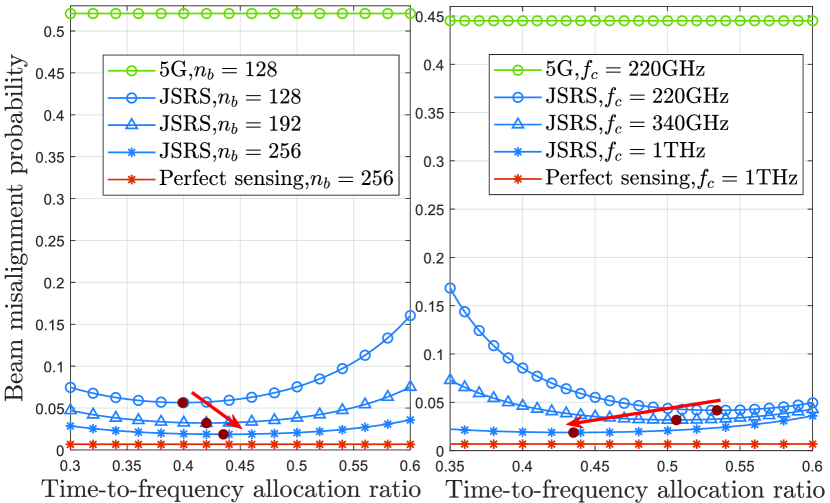
Figure 3: Time-to-frequency allocation ratio affected by (a) central frequency and (b) beamwidth.

VI-1 Perfect Sensing Case

As the upper bound, it stands for the ideal performance of the proposed sensing-aided scheme with no estimation error, labelled as Perfect sensing.

VI-2 5G Standard Sensing Case

As the benchmark, it represents the performance achieved with 5G-required sensing ability, labelled as 5G. Based on the 5GAA, the required sensing resolutions for general V2X use cases are set to $\Delta d_{b}=0.3{\rm{m}}$ in range and $\Delta V=1{\rm{m/s}}$ in velocity[42]. Substituting the resolutions into Lemma 1 and Theorem 2, we have the beam misalignment probability and coverage probability in 5G cases. In terms of the sensing cost in 5G cases, the RSs designed for channel estimation are considered as the major cost[36]. For the strictest comparison, we adopt the sparsest RS configuration, which is 1 OFDM symbol per slot[40]. The cost of sensing is then $\beta=1/14$.

VI-3 SSB-Based Sensing Case

For peer comparison, we select the single SSB-sensing scheme from work [24], labelled as SSB. In this case, SSBs are used for both blockage detection and user tracking. The motion and velocity resolutions are

$$\Delta d_{b}=A_{\theta}c/(2B_{\rm{SSB}}),\Delta v=c/(2f_{c}T_{\rm{SSB}}).$$

Because only the SSBs are used for sensing, the sensing cost ratio is $\beta=N_{\rm{SSB}}/N_{\rm{tot}}$.

For fairness, the available bandwidth is the same for all cases as the 5G-supported $B_{\rm{tot}}=1$GHz[36]. However, THz networks can practically support bandwidth up to hundreds of GHz, bringing in huge growth in throughput.

VI-A Beam Misalignment Probability

Averaged in tested cases, JSRS reduces the beam misalignment probability to $0.025$, showing an average improvement over $80\%$ and $70\%$ to that of 5G and SSB-sensing cases. We also reveal design insights into the sensing signal pattern design for minimizing the beam misalignment probability.

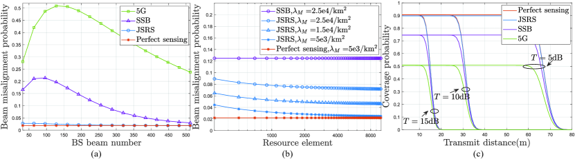
Figure 4: The performance enhancement of the JSRS scheme in the beam alignment and coverage probability.

Fig.3(a), (b) reveal design insights in the optimal time-to-frequency allocation ratio to achieve near-ideal performance with fixed sensing resources. Specifically, Fig.3(a) shows that utilizing the high angular resolution of narrower beams helps improve the beam alignment and reduce the cost of sensing. As shown in Fig.3(a), to cope with the frequent beam switches caused by narrower beams, the resources are more allocated to the time domain for higher velocity resolution, indicated as the increased allocation ratio. In contrast, Fig.3(b) shows that the resources are more allocated to bandwidth when using higher-frequency signals, thanks to their finer velocity resolution that spares more resources for frequency-domain range perception.

Fig.4(a) shows that JSRS-scheme significantly reduces the beam misalignment probability, compared to 5G and SSB cases. The near-ideal performance is achieved when $n_{b}\geq 256$ ($\theta\leq 1.41^{\circ}$). Thanks to the high angular resolution of narrow beams, after reaching the peak, the beam misalignment of the sensing-aided network decreases with narrower beams. It suggests that the JSRS scheme turns the disadvantages of sharp beams into advantages, allowing sensing-aided THz networks to use narrower beams to enlarge the coverage.

Fig.4(b) plots the JSRS benefit versus its cost. It shows that JSRS requires low sensing cost to provide promising assistance, and outperforms the 5G and SSB-based networks even with insufficient sensing resources. A near-ideal performance is achieved when $N_{\rm{RS}}\!\geq\!1500$, i.e., $T_{\rm{S}}\!=\!0.085{\rm{ms}},B_{\rm{S}}\!=\!0.15\rm{GHz}$, that is acceptable compared to the $10{\rm{ms}}$ frame duration and $1\rm{GHz}$ data bandwidth. Although the denser user increases the probability of beam misalignment, it can be compensated by increasing the sensing resource or using narrower beamwidth that both bring in more precise perception.

VI-B Coverage Probability

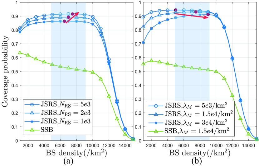
Figure 5: The BS density that maximizes the coverage probability affected by (a) sensing resource and (b) user density.

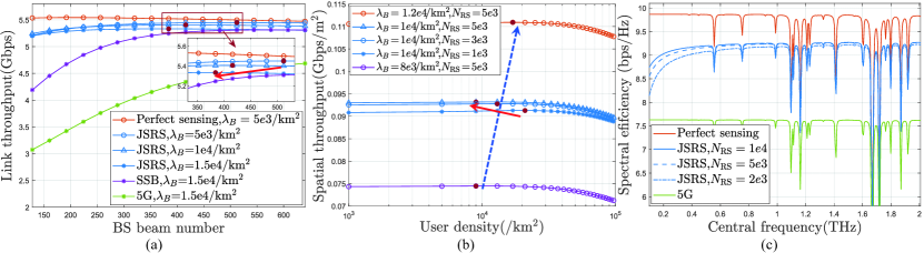
Figure 6: Network throughput analysis considering (a) the BS beam number, (b) user density and (c) central frequency.

As shown by Fig.4(c), under tested various scenarios, the JSRS-aided THz network achieves an average coverage probability of $90\%$, showing an increment by $75\%$, $20\%$ compared to the 5G-case and the SSB-sensing case respectively. It achieves near-ideal performance with a small difference in probability of around $0.007$. Satisfying a probability of $p_{\rm{cvp}}\geq 90\%$, JSRS-aided THz network covers around $60$m when the SINR threshold $T\!=\!5$dB, and reaches $30$m when $T\!=\!10$dB. Since sensing assistance cannot enhance signal power, the turning points of different cases are similar. But the JSRS scheme significantly enhances the coverage by improving the beam alignment, especially within the reachable range of the THz signals.

Fig.5 provides design insights in network deployment that maximizes the coverage probability. In tested cases, preferable BS density lies within $5e3-9e3/{\rm{km}}^{2}$, marked as the blue strips. Extra dense BS deployment causes a sharp drop in coverage, e.g., $\lambda_{B}\geq 1e4/{\rm{km}}^{2}$, suggesting that the THz network needs to restrain the node density to guarantee the link quality. Specifically, Fig.5(a) shows that the increase of sensing resources allows the network to deploy denser BSs, because higher sensing accuracy helps mitigate severe LoS-blockage effect on the dense network. Thus, the JSRS scheme can improve the spatial throughput of THz networks. As shown in Fig.5(b), the LoS blockage caused by denser users also degrades the coverage probability, requiring more BSs to support massive links. Increasing the BS density within a reasonable range not only shortens the transmission distance but also reduces the probability of LoS blockage, improving the received signal power with fewer link failures. Thus, deploying more BSs within a preferable range helps the network support more users.

VI-C Network Throughput

For fairness, we assume the same bandwidth for all cases. Averaged in various settings, the JSRS scheme realizes an increment of spatial throughput by $30\%$, compared to the network with 5G-sensing ability. It achieves near-ideal performance with a small gap of 3% difference per link throughput. Note that, the ultra-wide available THz bandwidth, i.e., $10-100{\rm{GHz}}$, can provide significant growth in the throughput of THz networks.

Fig.6(a) shows that the JSRS-aided network achieves over $5{\rm{Gbps}}$ link throughput, and near ideal performance is achieved when $n_{b}\geq 360$ in tested cases. It reveals the beamwidth trade-off between the enhanced sensing ability of narrower beams and its larger synchronization overhead. The red arrow indicates that a wider beamwidth is preferred to facilitate denser BS deployment, because they help reduce the synchronization overhead caused by frequent beam switches. Using narrower beams helps reduce the sensing overhead, thanks to their finer angular resolution. Thus, more time and bandwidth can be spared for data transmission to increase the throughput.

As plotted in Fig.6(b) JSRS-aided network achieves an average spatial throughput of $0.1-0.15{\rm{Gbps/m}}^{2}$. It shows the accessed user density needs to be balanced between the increased spatial throughput by massive links and the severer blockage effect that degrades link quality. Comparing the lines with round markers, the blue dashed arrow shows that the network is able to support more users with increased BS density, enhancing the spatial throughput. Comparing the lines of the same color, the red arrow shows that when moderately increasing the sensing resource, network can achieve comparable throughput with lower-density users, suggesting a higher throughput per link achieved at the user side.

Fig.6(c) plots the effect of THz molecular absorption on the spectral efficiency, suggesting the preferable THz transmission bands. JSRS-aided THz network achieves an average $9{\rm{bps/Hz}}$ spectral efficiency within the transmission windows, showing a $27\%$ improvement compared to that of the 5G case. It shows that with the increase of central frequency, the spectral efficiency is enhanced because of the more accurate velocity estimation of the higher-frequency signals. Also, at higher bands, using fewer sensing resources can achieve comparable spectral efficiency to that of using more sensing resources. Thus, networks operating at higher THz-band require less sensing cost, sparing resources for data transmission.

VII Conclusion

THz communication can support ultra-high-speed transmission, but it faces a coverage bottleneck that requires sharp beams to compensate for the propagation loss, which in turn brings in the narrow beam alignment challenge. In line with the 5G beam management, this paper proposes a JSRS scheme to assist THz beam alignment, which is highly compatible with the 5G air interface. Different from the traditional detect-and-correct method, JSRS helps the BS predict the impending beam switches and thus prevent beam misalignment, enhancing the network coverage probability. We provide a sensing signal configuration that determines the optimal time-to-frequency pattern to minimize beam misalignment with fixed sensing resources. Based on stochastic geometry, we derive coverage probability and spatial throughput expressions, which reveal insights into ISAC-THz network deployment and can be used to evaluate the performance gain from sensing. They also play important roles in follow-up studies on sensing resource allocation. In tested urban V2X scenarios, numerical results show that JSRS achieves near-ideal performance and effectively reduces average $80\%$ beam misalignment, and increases $75\%$ coverage probability, compared to 5G cases.

Appendix A

Recall (17), the beam misalignment probability is caused by the timeout and imperfect sensing.

First, we analyse the timeout probability $p_{\rm{B}}^{\rm{to}}$. Timeout happens when both the first and second close BSs are blocked, expressed as

$${\bf{E}}[p_{\rm{B}}^{{\rm{to}}}]={\bf{E}}[p_{\rm{B}}^{{r_{1}}}]{\bf{E}}[p_{{\rm{B}}}^{{r_{2}}}].$$ (43)

Suppose the distance to the first and second close BSs are $r_{1},r_{2}$ respectively. Using the PPP distribution probability, the probability density function (PDF) of $r_{1}$ and $r_{2}$ are respectively[27].

$${f_{{r_{1}}}}(r_{1})\!=\!2\pi{\lambda_{B}}r_{1}\exp(\!-\!{\lambda_{B}}\pi{{r_{1}}^{2}}),$$ (44a)

$${f_{{r_{2}}}}(r_{2})=2{\left({\pi{\lambda_{B}}}\right)^{2}}{{r_{2}}^{3}}{e^{-\pi{\lambda_{B}}{{r_{2}}^{2}}}},$$ (44b)

Based on our work[34], the LoS blockage probability is

$${p_{{\rm{B}}}}(r)=1-{e^{-({\lambda_{S}}+{\lambda_{M}})(r-2{r_{B}})2{r_{B}}}}.$$ (45)

Using (44), (45), the average LoS-blocked probability of the closet BS₁ and the second-close BS₂ are

$${\bf{E}}[p_{{\rm{B}}}^{{r_{1}}}] =\int_{2r_{\rm{B}}}^{+\infty}{p_{{\rm{B}}}}(r_{1}){f_{{r_{1}}}}(r_{1})dr_{1}$$

$$=1\!-\!{e^{2r_{B}w_{1}\!+\!\frac{{{w_{1}}^{2}}}{{4{\lambda_{B}}\pi}}}}\left[{{e^{-w_{2}^{2}}}\!-\!\frac{w_{1}}{2\sqrt{{\lambda_{B}}}}{\rm{erfc}}({w_{2}})}\right],$$ (46)

$${\bf{E}}[p_{{\rm{B}}}^{{r_{2}}}] =\int_{2r_{\rm{B}}}^{+\infty}{p_{{\rm{B}}}}(r_{2}){f_{{r_{2}}}}(r_{2})dr_{2}$$

$$=1-2{\left({\pi{\lambda_{B}}}\right)^{2}}{e^{2{r_{\rm{B}}}}}\int\nolimits_{2{r_{B}}}^{+\infty}{{r^{3}}{e^{-{w_{1}}r}}{e^{-\pi{\lambda_{B}}{r^{2}}}}}dr,$$ (47)

where $w_{1}\!=\!(\lambda_{S}\!+\!\lambda_{M})2r_{\rm{B}},w_{2}\!=\!2{r_{\rm{B}}}\sqrt{{\lambda_{B}}\pi}\!+\!\!\frac{w_{1}}{{2\sqrt{{\lambda_{B}}\pi}}}$, and the complementary error function ${\rm{erfc}}(x)=\tfrac{2}{\sqrt{\pi}}\int_{x}^{+\infty}e^{-x^{2}}dx$. Substituting (46), (47) into (43), we obtain the timeout probability.

Next, we analyse the probability of imperfect sensing-induced beam misalignment. As shown in Table II, $\Delta d_{b}\ll r_{\rm{B}}$, indicating that the range resolution is sufficient to detect the blockages. In this case, beam misalignment happens only when the BS underestimate the MT speed, and is unaware of the need to send an extra SSB burst to assist beam reselection. In other words, it happens when the actual speed $v>d_{b}/\tau$, but the estimated speed $\tilde{v}=v-\Delta v<d_{b}/\tau$, the probability of which can be expressed as

$$\begin{split}p_{{\rm{ve}}}^{\rm{s}}&=\mathcal{P}\left\{{v>\frac{{{d_{b}}}}{\tau},v-\Delta v<\frac{{{d_{b}}+\Delta{d_{b}}}}{\tau}}\right\}\\ &\stackrel{{\scriptstyle(a)}}{{=}}{e^{-{\mu_{g}}[(v-\Delta v)\tau-\Delta{d_{b}}]}}-{e^{-{\mu_{g}}v\tau}},\end{split}$$ (48)

where (a) results from the fact that the beam boundaries form Poisson Voronoi tessellation and the single beam coverage $d_{b}$ follows an exponential distribution with density $\mu_{g}=n_{b}\sqrt{\lambda_{B}}/\pi$[7]. The imperfect sensing-induced beam misalignment happens when the LoS link is unblocked but the BS underestimate the user speed. Using (46), (48), its probability is

$$p_{\rm{err}}=p_{\rm{ve}}^{\rm{s}}(1-{\bf{E}}[p_{\rm{B}}^{\rm{r_{1}}}]).$$ (49)

Substituting (46), (47), (49) into (17), we arrive at the beam misalignment probability

$$\!p_{\rm{m}}^{\rm{s}} \!=\!p_{{\rm{ve}}}^{\rm{s}}(1-{\bf{E}}[p_{{\rm{B}}}^{{r_{1}}}])+{\bf{E}}[p_{\rm{B}}^{{\rm{to}}}]$$ (50)

$$\!=\!{e^{\!-\!{\mu_{g}}v\tau}}\!\left[{{e^{{\mu_{g}}\!\left(\!{\Delta v\tau\!+\!\Delta{d_{b}}}\right)}}\!-\!1}\right]\!\left({1\!-\!{\bf{E}}[p_{\rm{B}}^{{r_{1}}}]}\right)\!+\!{\bf{E}}[p_{\rm{B}}^{{r_{1}}}]{\bf{E}}[p_{\rm{B}}^{{r_{2}}}].\!$$

Appendix B

Recalling the function to be minimized in (19a), we first obtain the spacings $U,V$ and then determine the ratio $\alpha$.

When fixing $N_{\rm{RS}}$, the larger insert spacing $U,V$, the smaller the $g(\alpha,U,V)$. Thus, the optimal $U_{\rm{opt}},V_{\rm{opt}}$ are the largest integers satisfying the constraints for sensing unambiguous range and velocity (see (19b), (19c)), given as

$$U_{\rm{opt}}=\left\lfloor{\frac{c}{{2{f_{{\rm{scs}}}}{d_{{\rm{max}}}}}}}\right\rfloor,V_{\rm{opt}}=\left\lfloor{\frac{c}{{2{f_{c}}{T_{\rm{sym}}}{v_{{\rm{max}}}}}}}\right\rfloor.$$ (51)

When the $U,V$ is fixed using (51), we notice that $g(U,V,\alpha)$ is a convex function about $\alpha$, the derivative of which on $\alpha$ is

$$\begin{split}\!\!g^{\prime}(U,V,\alpha)\!=\!-\frac{{c\tau\!{N_{{\rm{RS}}}}^{\!-\!\alpha}\!\ln({N_{{\rm{RS}}}})}}{{V2{f_{c}}{T_{{\rm{sym}}}}}}\!+\!\frac{{A_{\theta}}c{N_{{\rm{RS}}}}^{\alpha\!-\!1}\!}{{U2{f_{{\rm{scs}}}}}}\ln({N_{{\rm{RS}}}}).\end{split}$$ (52)

The optimal $\alpha_{\rm{opt}}$ appears when $g^{\prime}(U_{\rm{opt}},V_{\rm{opt}},\alpha)=0$, that is

$$\frac{{\tau{N_{{\rm{RS}}}}^{-{\alpha_{{\rm{opt}}}}}}}{{V\cdot 2{f_{c}}{T_{{\rm{sym}}}}}}=\frac{{{A_{\theta}}}}{{U\cdot 2{f_{{\rm{scs}}}}}}{N_{{\rm{RS}}}}^{{\alpha_{{\rm{opt}}}}-1}$$

$$\Leftrightarrow {N_{{\rm{RS}}}}^{2{\alpha_{{\rm{opt}}}}-1}=\frac{{U\cdot\tau{f_{{\rm{scs}}}}}}{{V\cdot{f_{c}}{T_{{\rm{sym}}}}{A_{\theta}}}}.$$ (53)

Calculating (53), we have the expression for the optimal $\alpha_{\rm{opt}}$

$$\begin{split}{\alpha_{{\rm{opt}}}}=\frac{1}{2}\left[{{{\log}_{{N_{{\rm{RS}}}}}}\frac{{U_{\rm{opt}}\cdot{f_{{\rm{scs}}}}\tau}}{{V_{\rm{opt}}\cdot{f_{c}}{T_{{\rm{sym}}}}{A_{\theta}}}}+1}\right].\end{split}$$ (54)

Appendix C

We calculate the coverage probability following the 4 steps summarized in Sec.V-B. Recall the coverage probability $p_{\rm{cvp}}(r)$ written by the CDF of $I_{\rm{eff}}(r_{1})$, as given in (33)

$${p_{{\rm{cvp}}}}(r_{1})\!=\!(1-p_{\rm{m}}^{\rm{s}})\mathcal{P}\left\{{I_{{\rm{eff}}}(r_{1})\!<\!{\frac{{{P_{\rm{C}}}(r_{1})}}{\mathcal{T}}}\!-\!P_{\rm{N}}^{{\rm{eff}}}(r_{1})}\!\right\}\!,\!$$ (55)

Since $p_{\rm{m}}^{\rm{s}}$ is obtained using Lemma 1, we derive the CDF of $I_{\rm{eff}}(r_{1})$ over the BS distribution, written as

$${p_{{\rm{cm}}}}=\mathcal{P}\left\{{{I_{{\rm{eff}}}(r_{1})<\frac{{{P_{\rm{C}}}(r_{1})}}{\mathcal{T}}-P_{\rm{N}}^{{\rm{eff}}}(r_{1})}}\right\}.$$ (56)

Thanks to the homogenous PPP distribution of the BSs, the effective interference $I_{\rm{eff}}(r_{1})$ to a typical user forms a shot-noise field[34]. Based on the its special properties, $p_{\rm{cm}}$ can be written as[28]

$$\begin{split}\!\!{p_{{\rm{cm}}}}\!=\!\!\mathop{\int}_{\!-\!\infty}^{\!+\!\infty}\!\!{{{\cal L}_{\rm{I}}}}\!\left({s,{r_{1}}}\right){\!e^{-2i\pi sP_{\rm{N}}^{{\rm{eff}}}(r_{1})}}\frac{{{e^{\frac{{2i\pi sP_{\rm{C}}({r_{1}})}}{\mathcal{T}}}}\!-\!1}}{{2i\pi s}}ds,\!\!\end{split}$$ (57)

where ${{\mathcal{L}}}_{\rm{I}}({s,{r_{1}}})={\bf{E}}\left[{e^{{-2i\pi s{I_{\rm{eff}}(r_{1})}}}}\right]$ is the Laplace functional of $I_{\rm{eff}}(r_{1})$. Using the expression of $I_{\rm{eff}}(r_{1})$ given in (30),

$$\begin{split}\!\!{{\cal L}_{\rm{I}}}(s,{r_{1}})\!\stackrel{{\scriptstyle(a)}}{{=}}\!{\bf{E}}\!\left[{e^{-2i\pi s\!\sum\!f({r_{i}})}}\right]\!\stackrel{{\scriptstyle(b)}}{{=}}\!\prod\limits_{i=1}^{{N_{{\rm{BS}}}(r_{1})}}\!{{{\bf{E}}}}\!\left[{{e^{-2i\pi sf({r_{i}})}}}\right],\end{split}$$ (58)

where in (a), we define $f(r_{i})$ for simplicity

$$f({r_{i}})=\left({{a_{i}}+K}\right)A{r_{i}}^{-2}{e^{-K{r_{i}}}},$$ (59)

in which the $\{a_{i}\}$ is a set of RVs with binomial distribution $\mathcal{P}\{a_{i}=1\}=p_{\rm{I}}(r_{i}),\mathcal{P}\{a_{i}=0\}=1-p_{\rm{I}}(r_{i})$ (see (24) for $p_{\rm{I}}(r_{i})$). Equation (b) in (58) results from the fact that the BSs are independently distributed. Using the probability generating functional (PGFL) of the PPP[28], (58) is then

$$\!{{\mathcal{L}}}_{\rm{I}}({s,{r_{1}}}\!)\!=\!\!\exp\!\left({\!-\!2\pi{\lambda_{B}}\!\!\mathop{\int}\nolimits_{r_{1}}^{\!+\!\infty\!\!}\!\!r\!\left(\!{1\!-\!{{\bf{E}}}[{e^{\!-\!2i\pi sf(r)}}]}\right)\!dr}\!\!\right)\!\!,\!$$ (60)

where the lower bound $r_{1}$ results from the fact that interferers farther than the connected BS₀. Substituting (32a), (32b) into (59), ${{\bf{E}}}[{e^{-2i\pi sf(r)}}]$ is then

$$\begin{split}\!{{\bf{E}}_{a\!}}[{e^{\!-\!2i\pi s\!f(r)}}]\!=\!{e^{\!-2i\pi\!sI_{{\rm{e}\!}}^{\rm{I}}(r)}}p_{\rm{I}}(r)\!+\!{e^{\!-2i\pi\!sI_{{\rm{e}}}^{{\rm{UI}}}(r)}}(1\!-\!p_{\rm{I}}(r)).\!\!\end{split}$$ (61)

Next, we utilize Euler’s formula, i.e., $e^{2i\pi x}=\cos(2\pi x)+i\sin(2\pi x)$[34], to separate the real and imaginary component, (61) is re-written as

$$\!{{\bf{E}}}[{e^{\!-\!2i\pi s\!f(r)}}] \!=\!\left[\cos(2\pi sI_{\rm{e}}^{\rm{I}}(r))\!+\!i\sin(2\pi sI_{\rm{e}}^{\rm{I}}(r))\right]{p_{I}}(r)$$ (62)

$$\!+\!\left[\cos(2\pi sI_{\rm{e}}^{\rm{UI}\!}(r))\!+\!i\!\sin(2\pi sI_{\rm{e}}^{\rm{UI}\!}(r))\right]\!(1\!-\!p_{\rm{I}}(r)).\!\!$$

Substituting (62) into (60), we have

$${{\cal L}_{I}}(s,r_{1})=\exp\left[-2\pi\lambda_{B}\left(f_{\rm{r}}(s)+i\cdot f_{\rm{i}}(s)\right)\right],$$ (63)

where $f_{\rm{r}}(s),f_{\rm{i}}(s)$ are the real and imaginary parts, written as

$$f_{\rm{r}}(s)= \mathop{\int}\nolimits_{2{r_{B}}}^{+\infty}r\left[{1-\cos(2\pi sI_{\rm{e}}^{\rm{I}}(r))\cdot{p_{I}}(r)}\right.$$

$$\left.{-\cos(2\pi sI_{\rm{e}}^{{\rm{UI}}}(r))\cdot(1-{p_{I}}(r))}\right]dr;$$ (64a)

$$f_{\rm{i}}(s)= \mathop{\int}\nolimits_{2{r_{B}}}^{+\infty}r\left[{\sin(2\pi sI_{\rm{e}}^{\rm{I}}(r))\cdot{p_{I}}(r)}\right.$$

$$\left.{+\sin(2\pi sI_{\rm{e}}^{{\rm{UI}}}(r))\cdot(1-{p_{I}}(r))}\right]dr.$$ (64b)

Using the parity of the trigonometric functions, we discover that $f_{\rm{r}}(s)$ is even and $f_{\rm{i}}(s)$ is odd. Thus, using the conjugate property of (60)), we have

$${\cal L}_{I}(-s,{r_{1}})=\exp\left[{-2\pi{\lambda_{B}}\left({f_{\rm{r}}(s)-i\cdot f_{\rm{i}}(s)}\right)}\right],$$ (65)

Substituting (63), (65) into (57), the integrand function of $p_{\rm{cm}}$ can be written as

$${f_{{\rm{int}}}}(s)={e^{-2\pi\lambda_{B}{f_{\rm{r}}}(s)}}\frac{{{e^{i\cdot{f_{2}}(s)}}-{e^{i\cdot{f_{1}}(s)}}}}{{2i\pi s}},$$ (66)

where $f_{1}(s),f_{2}(s)$ are given as

$${f_{1}}(s) =-2\pi\lambda_{B}{f_{\rm{i}}}(s)-2\pi sP_{\rm{N}}^{{\rm{eff}}}({r_{1}}),$$ (67a)

$${f_{2}}(s) =2\pi s\cdot\frac{{{P_{C}}({r_{1}})}}{\mathcal{T}}-2\pi\lambda_{B}{f_{\rm{i}}}(s)-2\pi sP_{\rm{N}}^{{\rm{eff}}}({r_{1}}),$$ (67b)

where $P_{\rm{N}}^{{\rm{eff}}}({r_{1}})$ is given in (31). Because $f_{i}(s)$ is odd, observing (67a), (67b)$,f_{1}(s),f_{2}(s)$ are odd functions about $s$. Noticing that the symmetry of the integral interval and substituting (66) into (57), we have

$$\begin{split}{p_{{\rm{cm}}}}&=\int_{-\infty}^{+\infty}{f_{{\rm{int}}}}(s)ds\\ &=\int_{0}^{+\infty}[{f_{{\rm{int}}}}(s)+{f_{{\rm{int}}}}(-s)]ds\\ &=\int_{0}^{+\infty}\frac{{{e^{-2\pi\lambda_{B}{f_{\rm{r}}}(s)}}}}{{\pi s}}\left[{\sin({f_{2}}(s))-\sin({f_{1}}(s))}\right]ds.\end{split}$$ (68)

Substituting (68) into (55), we arrive at

$$\!\!{p_{\rm{cvp}}}(r_{1})\! \!=\!(1\!-\!p_{\rm{m}}^{\rm{s}})\cdot{p_{{\rm{cm}}}}$$ (69)

$$\!=\!(\!1\!-\!p_{\rm{m}}^{\rm{s}}\!)\!\!\!\mathop{\int}\nolimits_{0}^{\!+\!\infty\!}\!\frac{{{e^{\!-\!2\pi\!\lambda_{B}\!f_{\rm{r}}(s)}}\!\!}}{{\pi s}}\left[{\sin({f_{2}}\!(s))\!-\!\sin({f_{1}}(s))}\right]\!ds.\!\!$$

References

- [1] F. Liu, Y. Cui, C. Masouros, J. Xu, T. X. Han, Y. C. Eldar, and S. Buzzi, “Integrated sensing and communications: Towards dual-functional wireless networks for 6G and beyond,” arXiv preprint arXiv:2108.07165, 2021.
- [2] I. F. Akyildiz, C. Han, Z. Hu, S. Nie, and J. M. Jornet, “Terahertz band communication: An old problem revisited and research directions for the next decade,” IEEE Trans. Commun., vol. 70, no. 6, pp. 4250–4285, 2022.
- [3] J. M. Jornet and I. F. Akyildiz, “Channel modeling and capacity analysis for electromagnetic wireless nanonetworks in the terahertz band,” IEEE Trans. Wirel. Commun., vol. 10, no. 10, pp. 3211–3221, 2011.
- [4] A. M. Elbir, K. V. Mishra, S. Chatzinotas, and M. Bennis, “Terahertz-band integrated sensing and communications: Challenges and opportunities,” arXiv preprint arXiv:2208.01235, 2022.
- [5] V. Petrov, M. Komarov, D. Moltchanov, J. M. Jornet, and Y. Koucheryavy, “Interference and SINR in millimeter wave and terahertz communication systems with blocking and directional antennas,” IEEE Trans. Wirel. Commun., vol. 16, no. 3, pp. 1791–1808, 2017.
- [6] Y. Wu, J. Kokkoniemi, C. Han, and M. Juntti, “Interference and coverage analysis for terahertz networks with indoor blockage effects and line-of-sight access point association,” IEEE Trans. Wirel. Commun., vol. PP, no. 99, pp. 1–1, 2020.
- [7] S. S. Kalamkar, F. Baccelli, F. M. Abinader Jr, A. S. M. Fani, and L. G. U. Garcia, “Beam management in 5G: A stochastic geometry analysis,” arXiv preprint arXiv:2012.03181, 2020.
- [8] W. Chen, L. Li, Z. Chen, H. H. Yang, and T. Quek, “Mobility and blockage-induced beam misalignment and throughput analysis for THz networks,” in 2021 IEEE Global Communications Conference (GLOBECOM). Spain: IEEE, 2021, pp. 1–6.
- [9] B. Ning, Z. Chen, W. Chen, Y. Du, and J. Fang, “Terahertz multi-user massive MIMO with intelligent reflecting surface: Beam training and hybrid beamforming,” IEEE Trans. Veh. Technol., vol. 70, no. 2, pp. 1376–1393, 2021.
- [10] B. Ning, Z. Chen, Z. Tian, C. Han, and S. Li, “A unified 3D beam training and tracking procedure for terahertz communication,” IEEE Trans. Wirel. Commun., vol. 21, no. 4, pp. 2445–2461, 2021.
- [11] H. Sarieddeen, N. Saeed, T. Y. Al-Naffouri, and M.-S. Alouini, “Next generation terahertz communications: A rendezvous of sensing, imaging, and localization,” IEEE Commun. Mag., vol. 58, no. 5, pp. 69–75, 2020.
- [12] C. Han, Y. Wu, Z. Chen, Y. Chen, and G. Wang, “THz ISAC: A physical-layer perspective of terahertz integrated sensing and communication,” arXiv preprint arXiv:2209.03145, 2022.
- [13] Z. Chen, C. Han, Y. Wu, L. Li, C. Huang, Z. Zhang, G. Wang, and W. Tong, “Terahertz wireless communications for 2030 and beyond: A cutting-edge frontier,” IEEE Commun. Mag., vol. 59, no. 11, pp. 66–72, 2021.
- [14] T. Wild, V. Braun, and H. Viswanathan, “Joint design of communication and sensing for beyond 5G and 6G systems,” IEEE Access, vol. 9, pp. 30 845–30 857, 2021.
- [15] O. Li, J. He, K. Zeng, Z. Yu, X. Du, Z. Zhou, Y. Liang, G. Wang, Y. Chen, P. Zhu et al., “Integrated sensing and communication in 6G: a prototype of high resolution multichannel THz sensing on portable device,” EURASIP J. Wirel. Commun. Netw., vol. 2022, no. 1, pp. 1–21, 2022.
- [16] J. A. Zhang, F. Liu, C. Masouros, R. W. Heath, Z. Feng, L. Zheng, and A. Petropulu, “An overview of signal processing techniques for joint communication and radar sensing,” IEEE J. Sel. Top. Signal Process., 2021.
- [17] F. Liu, L. Zheng, C. Yuanhao, C. Masouros, A. Petropulu, H. Griffiths, and Y. Eldar, “Seventy years of radar and communications: The road from separation to integration,” arXiv preprint arXiv:2210.00446, 10 2022.
- [18] C. Chaccour, W. Saad, O. Semiari, M. Bennis, and P. Popovski, “Joint sensing and communication for situational awareness in wireless THz systems,” arXiv preprint arXiv:2111.14044, 2021.
- [19] Y. Wu, F. Lemic, C. Han, and Z. Chen, “Sensing integrated DFT-spread OFDM waveform and deep learning-powered receiver design for terahertz integrated sensing and communication systems,” arXiv preprint arXiv:2109.14918, 2021.
- [20] S. Lu, F. Liu, Y. Li, K. Zhang, H. Huang, J. Zou, X. Li, Y. Dong, F. Dong, J. Zhu et al., “Integrated sensing and communications: Recent advances and ten open challenges,” arXiv preprint arXiv:2305.00179, 2023.
- [21] A. Zhang, M. L. Rahman, X. Huang, Y. J. Guo, S. Chen, and R. W. Heath, “Perceptive mobile networks: Cellular networks with radio vision via joint communication and radar sensing,” IEEE Veh. Technol. Mag., vol. 16, no. 2, pp. 20–30, Jun. 2021.
- [22] Z. Wei, Y. Wang, L. Ma, S. Yang, Z. Feng, C. Pan, Q. Zhang, Y. Wang, H. Wu, and P. Zhang, “5G PRS-based sensing: A sensing reference signal approach for joint sensing and communication system,” IEEE Trans. Veh. Technol., 2022.
- [23] B. Sun, B. Tan, M. Ashraf, M. Valkama, and E. S. Lohan, “Embedding the localization and imaging functions in mobile systems: An airport surveillance use case,” IEEE Open J. Commun. Soc., vol. 3, pp. 1656–1671, 2022.
- [24] W. Chen, L. Li, Z. Chen, T. Quek, and S. Li, “Enhancing THz/mmWave network beam alignment with integrated sensing and communication,” IEEE Commun. Lett., 2022.
- [25] K. Ji, Q. Zhang, Z. Wei, Z. Feng, and P. Zhang, “Networking based ISAC hardware testbed and performance evaluation,” IEEE Communications Magazine, 2023.
- [26] F. Baccelli and B. Błaszczyszyn, “Stochastic geometry and wireless networks: Volume I theory,” Foundations and Trends® in Networking, vol. 3, no. 3–4, pp. 249–449, 2010.
- [27] M. Haenggi, J. G. Andrews, F. Baccelli, O. Dousse, and M. Franceschetti, “Stochastic geometry and random graphs for the analysis and design of wireless networks,” IEEE J. Sel. Areas Commun., vol. 27, no. 7, pp. 1029–1046, 2009.
- [28] F. Baccelli, B. Blaszczyszyn, and P. Muhlethaler, “Stochastic analysis of spatial and opportunistic aloha,” IEEE J. Sel. Areas Commun., vol. 27, no. 7, pp. 1105–1119, 2009.
- [29] C. Wang and Y. J. Chun, “Stochastic geometric analysis of the terahertz (thz)-mmwave hybrid network with spatial dependence,” IEEE Access, vol. 11, pp. 25 063–25 076, 2023.
- [30] K. Humadi, I. Trigui, W.-P. Zhu, and W. Ajib, “User-centric cluster design and analysis for hybrid sub-6ghz-mmwave-thz dense networks,” IEEE Trans. Veh. Technol., vol. 71, no. 7, pp. 7585–7598, 2022.
- [31] M. Shi, X. Gao, A. Meng, and D. Niyato, “Coverage and area spectral efficiency analysis of dense terahertz networks in finite region,” China Commun., vol. 18, no. 5, pp. 120–130, 2021.
- [32] N. R. Olson, J. G. Andrews, and R. W. Heath, “Coverage and capacity of terahertz cellular networks with joint transmission,” IEEE Trans. Wirel. Commun., vol. 21, no. 11, pp. 9865–9878, 2022.
- [33] P. Ren, A. Munari, and M. Petrova, “Performance analysis of a time-sharing joint radar-communications network,” in 2020 International Conference on Computing, Networking and Communications (ICNC). IEEE, 2020, pp. 908–913.
- [34] W. Chen, L. Li, Z. Chen, and T. Q. Quek, “Coverage modeling and analysis for outdoor THz networks with blockage and molecular absorption,” IEEE Wirel. Commun. Lett., vol. 10, no. 5, pp. 1028–1031, May. 2021.
- [35] J. Kokkoniemi, J. Lehtomäki, and M. Juntti, “A discussion on molecular absorption noise in the terahertz band,” Nano Commun.Netw., vol. 8, pp. 35–45, 2016.
- [36] E. Dahlman, S. Parkvall, and J. Skold, 5G NR: The next generation wireless access technology. Academic Press, 2020.
- [37] Q. Zhang, X. Wang, Z. Li, and Z. Wei, “Design and performance evaluation of joint sensing and communication integrated system for 5G mmWave enabled CAVs,” IEEE J. Sel. Top. Signal Process., vol. 15, no. 6, pp. 1500–1514, 2021.
- [38] O. Tervo, T. Levanen, K. Pajukoski, J. Hulkkonen, P. Wainio, and M. Valkama, “5G new radio evolution towards sub-THz communications,” in 2020 2nd 6G Wireless Summit (6G SUMMIT), 2020, pp. 1–6.
- [39] T. Levanen, O. Tervo, K. Pajukoski, M. Renfors, and M. Valkama, “Mobile communications beyond 52.6 GHz: Waveforms, numerology, and phase noise challenge,” IEEE Wirel. Commun., vol. 28, no. 1, pp. 128–135, 2021.
- [40] (2021, Mar.) 3GPP TS 38.213 V16.5.0: ”NR: Physical layer procedures for control” (Rel-16). [Online]. Available: https://www.3gpp.org/ftp/Specs/archive/38_series/38.213/
- [41] K. M. Braun, “OFDM radar algorithms in mobile communication networks,” Ph.D. dissertation, Karlsruhe, Karlsruher Institut für Technologie (KIT), Diss., 2014, 2014.
- [42] (2021, Mar.) C-V2X Use Cases Volume II: ”Examples and Service Level Requirements”. [Online]. Available: https://5gaa.org/news/c-v2x-use-cases-volume-ii-examples-and-service-level-requirements/
- [43] I. Gordon, L. Rothman, R. Hargreaves, R. Hashemi, E. Karlovets, F. Skinner, E. Conway, C. Hill, R. Kochanov, Y. Tan et al., “The hitran2020 molecular spectroscopic database,” Journal of quantitative spectroscopy and radiative transfer, vol. 277, p. 107949, 2022.